An alternative origin for debris rings of planetesimals.

Abstract

Core Accretion (CA), the most widely accepted scenario for planet formation, postulates existence of $\sim$ km-sized solid bodies, called planetesimals, arranged in a razor-thin disc in the earliest phases of planet formation. These objects coagulate by collisions, eventually building planetary cores. In the Tidal Downsizing (TD) hypothesis, an alternative scenario for formation of planets, grain growth, sedimentation and formation of planetary cores occur inside dense and massive gas clumps formed in the outer cold disc by gravitational instability. As a clump migrates inward, tidal forces of the star remove all or most of the gas from the clump, downsizing it to a planetary mass body. Here we consider a rotating and/or strongly convective gas clump. We argue that such a clump may form not only the planetary core but also numerous smaller bodies. As an example, we consider the simplest case of bodies on circular orbits around the planetary core in the centre of the gas clump. We find that bodies smaller than $\sim 1$ km suffer a strong enough aerodynamic drag and thus spiral in and accrete onto the solid core rapidly. On the contrary, bodies in the planetesimal and larger size range lose their centrifugal support very slowly. We consider analytically and numerically the fate of these bodies after the host gas clump is disrupted. Planetesimals orbiting the protoplanetary core closely remain gravitationally bound to it; these may be relevant to formation of satellites of giant planets. Planetesimals on more distant orbits within the host clump are unbound from the protoplanet and are set on mildly eccentric heliocentric orbits, generically forming wide rings. These may correspond to debris discs around main sequence stars and the Kuiper belt in the Solar System. For the latter in particular, TD hypothesis naturally explains the observed sharp outer edge and the “mass deficit” of the Kuiper belt.

1 Introduction

1.1 Planet formation: bottom-up or top-down?

Core Accretion (CA) theory (Pollack et al., 1996; Alibert et al., 2005) posits that planet formation starts when some of the dust grains in the protoplanetary disc grow and sediment to the disc midplane. This step is then followed by a less well understood one in which much larger solid objects of a few km or more are made (cf. Youdin & Shu, 2002; Johansen et al., 2007). These rocky objects, called “planetesimals”, then co-coagulate into terrestrial-like planetary cores (Safronov, 1972). These cores continue to gain mass by mergers and accretion of planetesimals. If the cores are still embedded in the parent gaseous disc, then a gas atmosphere builds up around the cores. When the solid core mass exceeds a few to a few tens Earth masses, the atmosphere becomes self-gravitating and collapses hydrodynamically to much higher densities, forming a proto-giant gas planet (Mizuno, 1980; Stevenson, 1982; Rafikov, 2006). This model may be termed a bottom-up scenario for planet formation.

An alternative top-down scenario for the origin of planets is also physically plausible, although it is currently much less developed (Boley et al., 2010; Nayakshin, 2011a). The very first step in this “Tidal Downsizing” (TD) scheme is reminiscent of formation of stars, that is the Jeans self-gravitation instability of a gas cloud/clump (for example, see Larson, 1969). The cloud is however much less massive, e.g., its mass is around the opacity fragmentation limit of $\sim 10M_{J}$ (Rees, 1976; Nayakshin, 2010b; Forgan & Rice, 2011), and is born inside a gas disc orbiting the parent star (e.g., Boss, 1997). The second step in TD scenario is similar to the first one in CA model, e.g., grains grow and sediment. However, this process occurs inside the gas clumps rather than the whole of the disc, where the densities are much lower (cf. simulations of Cha & Nayakshin, 2011). A massive solid core therefore forms inside the gas clump (Boss, 1998; Helled & Schubert, 2008; Nayakshin, 2011a). Rapid inward radial migration of the gas clump (Vorobyov & Basu, 2005, 2006; Machida et al., 2011; Michael et al., 2011; Baruteau et al., 2011) then expose the clump to the ever increasing tidal force of the parent star. Removal of all or a part of the original gas cloud by tidal forces of the star may hypothetically leave behind both terrestrial-like and gas giant planets (Boley et al., 2010; Nayakshin, 2010a). Note that while the combination of these physical steps is a very recent development, the TD hypothesis may be viewed as a physics-upgraded version of the gravitational disc instability model (GI; e.g., Boss, 1997; Rice et al., 2005; Rafikov, 2005). The complicated fate of gas clumps in a self-gravitating disc was also discussed by Mayer et al. (2004), who also noted that these clumps may be tidally disrupted if they migrate inward. Furthermore, except for the crucial step of the radial migration of the gas clump, the TD scheme is similar to ideas of McCrea & Williams (1965).

The current status of TD planet formation hypothesis is best described as “work in progress”. Progress is being made in terms of building more self-consistent time-dependent models of the protoplanetary discs with embedded massive gas clumps (e.g., Boley et al., 2011; Nayakshin & Lodato, 2011); addressing the surprising high temperature content of Solar System comets (Vorobyov, 2011; Nayakshin et al., 2011); chemistry of self-gravitating discs (Ilee et al., 2011); the “hot” super-Earth planets (Nayakshin, 2011b); and rotation of the Solar System terrestrial planets (Nayakshin, 2011c). Despite this, no detailed statistical predictions in the spirit of population synthesis models of Ida & Lin (2008, 2010) have yet been made. The TD hypothesis thus cannot yet be compared with exoplanetary data in detail.

One promising way to constrain the TD hypothesis observationally is via observations of the early “embedded” phase of star (and potentially planet) formation (Dunham & Vorobyov, 2012), especially with the advent of the ALMA telescope when resolving individual massive gas clumps in large $R\lower 2.15277pt\hbox{$\;\buildrel>\over{\sim}\;$}50$ AU discs around young protostars may become possible.

1.2 Can solid debris constrain planet formation theories?

Planets are not the only bodies orbiting their host stars: solid bodies from microscopic dust to sub-terrestrial planet size objects such as Pluto also form during planet assembly both in the Solar System and around other nearby stars. In particular, Solar System contains several repositories of $\lower 2.15277pt\hbox{$\;\buildrel>\over{\sim}\;$}1$ km sized solid bodies – the asteroid belt, the Kuiper belt, the scattered disc and the Oort cloud of long-period comets. Starting from the discovery of the infrared excess beyond 12$\mu$m around Vega by IRAS (Aumann et al., 1984), circum-stellar dust disc are commonly found around pre- and main sequence stars (Zuckerman, 2001; Wyatt, 2008). Since microscopic dust in the discs around main sequence dust should be blown away rapidly due to radiation pressure from the parent stars, a continuous replenishment source for the dust is required (Wyatt et al., 2007). The universally accepted picture is that the circum-stellar dust results from a fragmentation ”cascade” (e.g., Hellyer, 1970; Wyatt et al., 2007; Wyatt, 2008) of larger solid bodies such as comets and asteroids. This view is reinforced by observations of dust resulting from such fragmentation cascades in our own Solar System (Nesvorný et al., 2003; Nesvorný et al., 2010), and also by the signatures of collisional sculpting of the asteroid belt (e.g., Bottke et al., 2005).

It is obvious that the solid debris around stars has a rather natural explanation in the context of the CA theory: these bodies are the planetesimals and “half-grown” planetary embryos that did not get consumed or ejected completely from the system by the growing planets. The question we pose in this paper is this: Can TD hypothesis produce solid debris too, and if so, how do the properties of that debris differ from the CA model?

We shall argue below that it is economical and logical to have all smaller solid objects to be born inside the same “parent” gas clumps where the terrestrial-like solid cores grow. We arrive at these conclusions based on the following ideas. In the 1D spherically symmetric models of Helled and co-authors, and in Nayakshin (2011a), only one central core is formed. However, (Nayakshin, 2011b) has shown that specific angular momentum of the grains may be too large to allow gravitational collapse into just one massive body. Gravitational collapse of a rapidly rotating cloud may result in formation of not only the central body but also a number of smaller objects possibly orbiting the larger one in a centrifugally supporting disc. The objects may fragment or grow further due to subsequent collisions. In addition, the formation of the solid core releases a significant amount of energy into the surrounding gas (Nayakshin, 2011a), which stirs up strong convective motions. This second effect may also promote formation of additional solid bodies by gravitational collapse of smaller grain-dominated regions (cf. §3.6.2 and 3.6.3 of Nayakshin, 2010b) on chaotically oriented orbits.

The next logical step in our picture is the disruption of the parent gas clump, as required by the TD hypothesis. We show below that the solid debris population within the clump can be divided into two groups: one bound to the planetary core (be it terrestrial-like or more massive by that point), and the other to the host gas clump. Upon disruption of the clump the first group “survives” and becomes planet’s satellites; the other group gets disrupted and dispersed with the gas. Generically, the second population of debris forms a “disruption ring” centred on the location of the host gas clump disruption.

Below we study analytically and numerically (for three representative cases) the properties of the post-disruption orbits of the planetesimal debris. We start in §2 by discussing the likely structure of the gas clump before the disruption. We show that there are two possible ways of the host clump disruption – either tidally or due to an internal energy release by the growing protoplanetary core itself. We estimate the minimum mass of the core being able to disrupt the host clump to be $\sim 10$ Earth masses.

In §3.1 we consider the aerodynamic drag acting on the solid bodies within the host clump. We find that bodies smaller than $\sim$ 1 cm and larger than $\sim 1$ km stand a good chance of remaining “independent” after the clump disruption compared with the bodies between these size limits: these suffer strong drag from the gas and must end up joining the protoplanetary core in the centre of the gas clump. In §3.4 we consider analytically the kind of orbits that the large solid bodies obtain after the gas clump disruption. §4 describes the set up of our numerical experiments. Several following sections present the numerical results, with §5 showing the gas flow, §§6 and 7 focusing on the population of unbound and bound solid bodies, respectively. §8 contains a discussion of the main results of our paper.

2 Host clump structure and disruption

2.1 Setup and terminology

For definitiveness, we consider a host gas clump of $M_{\rm hc}=5M_{J}$ mass in the numerical part of the paper. We assume that the initial density and temperature profiles are that of a polytropic sphere with the polytropic index $n=5/2$ as appropriate for a molecular hydrogen-dominated gas in the temperature range from a few hundred K to about 1500 K (Boley et al., 2007). The clump is initially located at $R=40$ AU on a circular orbit around the star of mass $M_{*}=1M_{\odot}$.

We shall refer to the host gas clump as such to distinguish it from the solid planetary core, which we frequently call “planet”. The planet (of mass $M_{\rm p}=10{\,{\rm M}_{\oplus}}$) is treated as a point mass in this paper. We assume that the density of the planet is much higher than that of the host clump. Therefore, the internal structure of the planet is not affected by the host gas clump disruption. We note that this setting does not require the planet to consist of high-Z material only; volatiles could be present also as long as their densities are much higher than the tidal density, $M_{*}/2\pi R^{3}$.

2.2 Clump disruption by tidal forces

We study two limiting cases of clump disruption. In the case of disruption due to tidal forces from the star, the host clump fills its Roche lobe at the start of the simulation, time $t=0$. The size of the Roche lobe (Hill’s radius) at this location is

$$r_{h}=R\left(\frac{M_{\rm hc}}{3M_{*}}\right)^{1/3}\approx 4.7\;\mbox{AU}\;.$$ (1)

A polytropic cloud with the clump mass $M_{\rm hc}=5M_{J}$ and the clump radius, $r_{\rm hc}$, satisfying $r_{\rm hc}=r_{h}$ has central temperature $T=195$ K, for reference.

The mass-radius relation of a polytropic cloud is given by

$$r_{\rm hc}\propto M_{\rm hc}^{\frac{1-n}{3-n}}\propto M_{\rm hc}^{-3}\mbox{ for }n=5/2\;.$$ (2)

This implies that the host clump expands rapidly as mass is lost. We therefore expect a prompt tidal disruption of such a host clump by Roche lobe overflow: $r_{\rm hc}$ increases while $r_{h}$ decreases as $M_{\rm hc}$ drops.

We shall add to this that the stabilising effect of the host clump outward migration due to the mass exchange between the gas clump and the star, discovered by Nayakshin & Lodato (2011), does not occur in our simulations because the clump is destroyed rather rapidly in all of the simulations below. In addition, we find that disruption proceeds via both L1 and L2 points, in contrast to what is found for much more gentle “hot disruptions” at $R\sim 0.1$ AU separations by Nayakshin & Lodato (2011). For both of these reasons there is no outward torque on the host clump; the tidal disruption has a runaway character.

2.3 Disruption by an internal energy release

In the second class of models we consider here, the clump’s initial radius is smaller than the Hill’s radius $r_{h}$. In particular, for the two simulations presented below, we set the initial central temperature to $T=500$ K, which corresponds to the clump’s initial radius of $r_{\rm hc}=1.84$ AU. We then assume that a sudden burst of energy release occurs in the centre of the clump. Physically, we relate the burst to the assembly of the planetary core, as is found in 1D simulations of Nayakshin (2011a). In detail, the energy released by the solid core is passed to the surrounding gas by radiative diffusion. If the radiative diffusion time scale is longer than the planetary core’s assembly time and the injection energy is large enough then even an isolated gas clump may be disrupted. An example of this is simulation M0$\alpha$3, Figures 5 to 7 in Nayakshin (2011a).

We estimate the energy released by the planetary core to be about its binding energy,

$$E_{\rm bind,c}\approx\frac{GM_{p}^{2}}{2r_{p}}=5\times 10^{40}\;\hbox{erg}\;\left(\frac{M_{p}}{10M_{\oplus}}\right)^{5/3}\rho_{p}^{1/3}\;,$$ (3)

where $G$ is the gravitational constant, and $\rho_{p}$ is the solid core density in g cm^-3.

Let us now compare the core’s binding energy with the minimum amount of energy needed to disrupt the host clump. The total energy of a polytropic gas clump, $E_{\rm hc}$, is given by

$$E_{\rm hc}=-\frac{3-n}{5-n}\frac{GM_{\rm hc}^{2}}{r_{\rm hc}}\;.$$ (4)

For simplicity we assume that the clump remains polytropic after the energy injection (which is not obvious at all; we will come back to this later) with same $n$ but a different adiabatic constant. The energy input sufficient to disrupt the clump, $\Delta U_{0}$ is the energy needed to inflate the clump to the point of its tidal disruption, i.e., when $r_{\rm hc}$ increases and becomes equal to the Hill’s radius, $r_{h}$. Thus,

$$\Delta U_{0}=\frac{3-n}{5-n}\left(1-\frac{r_{\rm hc}}{r_{h}}\right)\;\frac{GM_{\rm hc}^{2}}{r_{\rm hc}}\;.$$ (5)

For reference, $GM_{\rm hc}^{2}/r_{\rm hc}\approx 2.4\times 10^{41}$erg for clump mass $M_{\rm hc}=5M_{J}$ and clump radius $r_{\rm hc}=1.84$ AU.

As energy released by the core heats the surrounding gas, it is instructive to compare the required energy injection $\Delta U_{0}$ with the initial total internal energy of the host clump, $U_{0}$:

$$\frac{\Delta U_{0}}{U_{0}}=-\left(1-\frac{3}{n}\right)\left(1-\frac{r_{\rm hc}}{r_{h}}\right)\;.$$ (6)

In the limit of the initially small host clump, $r_{\rm hc}\ll r_{h}$, the disruption energy is $\Delta U_{0}=0.2U_{0}$ for $n=5/2$. In the case under consideration, $r_{\rm hc}=1.84$ AU, and $r_{h}=4.7$ AU, and thus $\Delta U_{0}=0.123U_{0}$.

From the following we conclude that the energy required to unbind the host gas clump is of the order of $3\times 10^{40}$ erg. This is of the same order as the binding energy of the planetary core of mass $M_{p}=10M_{\oplus}$. Therefore, we see that, to disrupt the host clump with the energy released by the planetary core, the mass of the core must be at least $M_{p}\sim 10M_{\oplus}$. We also note in passing that the similarity of this mass to the critical solid core mass in the CA theory (e.g., Mizuno, 1980; Stevenson, 1982) seems to be a pure coincidence. While the minimum mass capable of disrupting the gas host clump is the function of the conditions in that clump (mass, age, opacity, etc.), the CA critical mass is a function of the core’s surroundings – the location from the star, opacity and the planetesimal accretion rate from the surrounding protoplanetary disc (e.g., Rafikov, 2011).

3 Solids within the clump

Nayakshin (2010b, 2011a) finds that when grains contained in the host clump grow by the hit-and-stick mechanism to sizes of the order of $s\sim 10$ cm, their sedimentation within $\sim 1000$ years becomes possible (see also McCrea & Williams, 1965; Boss, 1998). Accumulation of these to the centre of the clump creates a region dominated by grains rather than by gas. This region, called “grain cluster” by Nayakshin (2010b) then becomes gravitationally unstable and collapses to form a massive core composed of high-Z materials.

As argued in §1.2, due to rotation and chaotic convective gas motions in the centre of the host clump, one may expect numerous smaller bodies to form in the centre of the clump as well. It is the fate of these bodies that interests us here.

3.1 Aerodynamic drag in the host clump

We shall now consider what happens to solids of different sizes, $s$, from microscopic grains to asteroid-sized bodies, if they are placed within the host clump. As we shall see, due to the aerodynamic drag that these solids suffer, small grains ($s\lower 2.15277pt\hbox{$\;\buildrel<\over{\sim}\;$}0.1-1$ cm) are nearly frozen in with the gas, so have to follow its motion, whereas bodies larger than $s\sim 1$ km experience negligible friction with the gas. Bodies in the intermediate size range are most likely to end up joining the solid core. The smaller and the larger objects may survive the gas clump disruption and become either planet satellites or independent bodies in heliocentric orbits.

To quantify this discussion, we model the host gas clump in this section only as in the analytical model of Nayakshin (2010a), which shows that the outer radius of the host clump is approximately independent of the clump’s mass, $r_{\rm hc}=0.8$ AU $k_{*}^{1/2}(10^{4}\mbox{yr}/t_{\rm hc})^{1/2}$, where $t_{\rm hc}$ is the host clump’s age, and $k_{*}$ is dimensionless opacity (cf. §2.1 of Nayakshin, 2010a). The age of the host clump chosen for the representative calculation below is $10^{4}$ years, the mass is $10M_{J}$, and opacity $k_{*}=1$. Note that in detail the structure of the host clump is different from that of the gas clumps we consider in the numerical of the paper, but the main conclusions that we reach in this section are qualitatively unaffected by this.

For simplicity, clump rotation is neglected in this section, but we note that results for rotating gas clumps are actually quite similar as long as gas pressure is the main means of support against gravity for the host clump (in the opposite case the gas clump would be unstable to various fluid instabilities; see, e.g., chapter 7 of Shapiro & Teukolsky, 1983).

Our goal here is to calculate how long it takes for a grain of size $s$ and a given initial condition for the grain position and velocity to settle to the centre of the clump due to aerodynamic friction with the gas. To achieve this goal, we solve for the grain’s motion within the host clump using the formulae of Weidenschilling (1977) for the aerodynamic forces acting on the grains. This allows us to calculate the radial sedimentation velocity of the grain, $v_{r}$, and define the sedimentation time as

$$t_{\rm sed}={r\over|v_{r}|}\;.$$ (7)

where $r$ is distance to the clump’s centre. For solids released from rest results of such calculations are presented in fig. 2 of Nayakshin et al. (2011). Here we present a very similar calculation for dust grains that are on initially circular orbits around the host gas clump’s centre.

Figure 1 shows the sedimentation time scale for grains released on circular orbits with initial radii $r$ of 0.02, 0.1 and 0.5 times $r_{\rm hc}$ for the blue dot-dashed, brown dashed and black solid curves, respectively. For comparison, the red dash-triple-dot curve shows the grain sedimentation time for a grain released from rest, as in Nayakshin et al. (2011).

Without rotation, grains larger than a few cm manage to sediment to the centre of the gas clump within its age. Smaller grains are tightly bound to the gas, and if the host is disrupted, these grains are released into the disc around the protoplanet. The grains closest to the solid core could have been thermally reprocessed into crystalline materials; mixing these with surrounding disc’s ices and incorporating into comets may explain their puzzling compositions (Vorobyov, 2011; Nayakshin et al., 2011).

In a purely spherical geometry with no rotational support for grains, large grains ($s\lower 2.15277pt\hbox{$\;\buildrel>\over{\sim}\;$}1$ m) fall into the centre and join the solid core on the free-fall time, which for a constant density model clump is constant with radius (cf. the horizontal part of the red dash-triple-dot curve).

For grains on circular orbits, however, centrifugal force balances gravity, and the grains sediment only because of a gradual angular momentum loss due to aerodynamic forces. These forces become progressively less important for larger grains, and therefore the grain sedimentation time increases with $s$ again (cf. the black, the brown and the blue curves in Fig. 1). As a result, grains larger than 1-10 km may orbit the centre of the clump for times comparable with the clump’s lifetime (which we assume of the same order as the clump’s age here, as presumably the clump continues to migrate inward at roughly same migration speed).

Concluding, we see that solid objects larger than a few km in size do not necessarily contribute to growth of the solid planetary core as it may take too long for these bodies to spiral into the core: the host clump is likely to be disrupted before such an inspiral occurs.

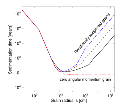
Figure 1: Sedimentation times versus grain size for grains set initially on circular orbits, except for the red dash-triple-dot curve which is for a grain released from rest.

3.2 On planetesimal birth and sizes

In this paper we do not simulate the phase of planetesimal formation due to numerical challenges. Previous simulations of the whole proto-planetary disc by Cha & Nayakshin (2011) lacked numerical resolution (to resolve smaller objects) and resulted in formation of single self-bound massive ($M\lower 2.15277pt\hbox{$\;\buildrel>\over{\sim}\;$}$ a few ${\,{\rm M}_{\oplus}}$) clusters of dust particles inside the gas clumps. These were held from a further self-gravitational collapse artificially by employing a finite gravitational softening length in the simulations. Increasing numerical resolution further (that is, the number of SPH and dust particles) by up to several orders of magnitude is needed to resolve small, e.g., $\lower 2.15277pt\hbox{$\;\buildrel<\over{\sim}\;$}0.01$ AU scales, on which planetesimals we are interested here could form. This is beyond our present numerical capabilities.

Figure 1 shows a difficulty for formation of planetesimals in the TD scheme, very much similar in nature to the well known “metre-size barrier” for the planetesimal growth in the protoplanetary discs (Weidenschilling, 1977). In the CA theory, aerodynamic coupling with the gas makes $\sim$ metre-sized boulders migrate radially inward in the disc, so that they are probably lost to the protostar before they become planetesimals.

Similarly, Figure 1 shows that solids of intermediate sizes migrate radially inward very rapidly even if they are initially set on circular orbits around the centre of the host gas clump. Such objects thus must join the massive solid core there. To arrive at km-sized and larger bodies that suffer much weaker aerodynamic drag, smaller grains must thus somehow “jump” from being small to being large without suffering the aerodynamic drag.

We leave a detailed study of this issue to a future paper, but make some suggestions on how this difficulty may be avoided. First of all, again reminiscent of the well known ideas in the CA theory context, channels for a rapid growth of solids may be available: via self-gravitational instability (Safronov, 1972; Goldreich & Ward, 1973) of dust-dominated regions (although not in necessarily in the shape of a disc), or via turbulence (e.g., Youdin & Goodman, 2005; Johansen et al., 2007; Cuzzi et al., 2008).

Secondly, and unlike the CA “metre-size barrier” problem, here it is much less clear that aerodynamic drag does make all the medium-sized solids to accrete onto the central object. In the case of a proto-planetary disc (the CA model), the protostar contains almost all the mass and is thus the natural central (nearly) point-mass around which the disc rotates. Grains migrating inward must therefore end up in the star. In the TD case, however, the mass of the “massive” solid core we are thinking about is measured in Earth masses, which is $\sim 10^{-3}$ of the total host gas clump mass. If there are turbulent or convective motions in the inner region of the clump (which is almost a certainty), then the solid core itself will be affected by the gas motions through its coupling to the gas via gravity of the latter. Thus it may not “sit” in the centre of the clump accreting all the medium-sized solids sedimenting there. Furthermore, motion of the grains would also be affected, with turbulent and convective motions of gas dragging the grains around. There is clearly a limit here; too much of turbulence would prevent grains from sedimenting into the centre in the first place, but moderate turbulent motions may be expected to delay grain accretion onto the solid core and lead to formation of new condensation centres which perhaps would lead to formation of the larger planetesimals that we study in the rest of the paper.

It would also be desirable to understand just how large the planetesimals formed inside the host gas clump are likely to be. Following §3.6.2 and 3.6.3 of Nayakshin (2010b), we find that the linear extent of the region of the gas cloud within which the first gravitational collapse of grain-dominated regions could occur is about $\sim 0.1$ times the size of the gas clump. For the total grain mass in the collapsing region of $10{\,{\rm M}_{\oplus}}$, the expected velocity dispersion of fragments formed by collapse is then $\sim 0.5$ km s${}^{{}_{1}}$.

Now, collisions of large planetesimals of equal size, $a$, would lead to their fragmentation if the collision velocity ($\sim$ the velocity dispersion calculated above) is larger than the escape velocity from the surface of the planetesimal (e.g., Stewart & Leinhardt, 2009). This would then suggest that collisions of equal size bodies inside the “grain sphere” would split planetesimals smaller than about 1000 km, while larger bodies would “stick”. One however need to estimate the frequency of such collisions. Assuming that the grain sphere fragments into bodies of approximately equal size, we find that all the planetesimals would have had at least one catastrophic (shattering) collision within a thousand years inside the grain sphere for $a\lower 2.15277pt\hbox{$\;\buildrel<\over{\sim}\;$}100$ km. Collisions with smaller bodies – fragments of the “original” planetesimals – increase this collision rate estimate further. We thus conclude that expected sizes of planetesimals surviving the dense environment of the inner region of the clump are at least a few hundred km. Presumably both smaller and larger solid objects could then be obtained over much longer time scales by collisional evolution of the disrupted population.

3.3 Planet’s influence radius: bound and unbound debris

Having understood the range of body sizes ($s\lower 2.15277pt\hbox{$\;\buildrel>\over{\sim}\;$}1$km) that may be considered as independent for the duration of the host clump, we now shift out attention to what may happen when the host clump is disrupted. In detail the answer on this question is quite complicated as it depends on the nature of planetesimal orbits within the clump and the exact way the clump is disrupted. However, for not too eccentric orbits, we can divide the planetesimal population on those that are “close” and those that are “far” from the solid planetary core. The former have a fair chance of remaining bound to the solid core when the host clump is disrupted, and the latter become unbound independent objects.

To quantify this, consider the simplest setting, placing a solid core of mass $M_{p}$ in the centre of the gas clump and setting planetesimals on circular orbits around the planet. The rotation of the planetesimal’s disc is assumed prograde with respect to the orbit of the host clump around the star. The circular speed of the planetesimals around the planet is given by

$$v_{\rm circ}^{2}=G{M_{p}+M(r)\over r}\;,$$ (8)

where $M(r)$ is the gas mass enclosed inside radius $r$ (distance from the centre of the host clump).

If planet’s mass is low enough to build up a massive self-gravitating atmosphere around it (which is expected to be the case for an adiabatic young gas clump where the critical core mass is above 100 ${\,{\rm M}_{\oplus}}$; see Perri & Cameron, 1974), then the gas density is nearly constant in the clump’s centre. Let us call that central density $\rho_{0}$; thus $M(r)\approx(4\pi/3)\rho_{0}r^{3}$. We can now define the planet influence radius, $r_{i}$, such that $M(r_{i})=M_{p}$. Apparently,

$$r_{i}=\left[{3M_{p}\over 4\pi\rho_{0}}\right]^{1/3}\;.$$ (9)

Note that since $r_{\rm hc}=(3M_{\rm hc}/4\pi\rho_{\rm mean})^{1/3}$, where $\rho_{\rm mean}$ is the mean density of the host clump, then we have

$$r_{i}\approx r_{\rm hc}\left({M_{p}\over M_{hc}}\right)^{1/3}\left({\rho_{\rm mean}\over\rho_{0}}\right)^{1/3}=0.18\;r_{\rm hc}\left({\rho_{\rm mean}\over\rho_{0}}\right)^{1/3}$$ (10)

Solids inside $r_{i}$ are gravitationally bound mainly to the planet, whereas those outside are bound by the enclosed gas. We expect that when the host clump is disrupted, objects within $r_{i}$ remain bound to the solid planet whereas objects outside this radius become unbound from the planet.

3.4 Post-disruption orbits for unbound debris

We now build an approximate analytical theory for the orbits of the planetesimals after the host clump tidal disruption. To this end we assume that gas clump disruption is instantaneous. We also assume that solids within $r_{i}$ remain bound to the planet and continue to follow its motion around the central star, and we concentrate here only on solids outside the influence radius.

Before the disruption, the position of a planetesimal with respect to the star is given by $\mathbf{R}+\mathbf{r}$, where $\mathbf{R}$ is the vector connecting the star with the centre of the gas clump (solid planet’s location), and $\mathbf{r}$ is the vector connecting the centre of the host clump with the given planetesimal. The instantaneous velocity of the planetesimal is also comprised of two parts, one due to the heliocentric Keplerian motion of the gas clump, $\mathbf{V}$, and the other given by the circular prograde rotation velocity, $v_{\rm circ}$, around the centre of the host clump.

We now call $\mathbf{V+\Delta v}$ the planetesimal’s velocity right after the host clump disruption. Physically, $\mathbf{\Delta v}$ is the velocity with which planetesimal becomes unbound, and may be called a velocity “kick”. We expect that $0<\Delta v<v_{\rm circ}$ for the energy conservation reasons.

We shall now calculate the new heliocentric orbit of the planetesimal by considering its specific energy and angular momentum. The specific energy and specific angular momentum of the host gas clump before the disruption are $E_{0}=-GM_{*}/2R$ and $\mathbf{L_{0}=R\times V}$, respectively. The post-disruption specific energy, $E$, and specific angular momentum, $\mathbf{L}$, of the planetesimal are

$$E = -\frac{GM_{*}}{|\mathbf{R}+\mathbf{r}|}+\frac{1}{2}\left|\mathbf{V}+\mathbf{\Delta v}\right|^{2},$$ (11)

$$\mathbf{L} = (\mathbf{R}+\mathbf{r})\times(\mathbf{V}+\mathbf{\Delta v}),$$ (12)

where, $M_{*}$ is the mass of the central protostar. Decomposing these expressions into Taylor series with respect to small parameters $r/R$ and $\Delta v/V$, up to the linear terms only, and writing $E\approx E_{0}+\delta E$, $L^{2}\approx(L_{0}+\delta L)^{2}$ (the latter is possible since $\mathbf{\Delta v}$ is in the clump’s orbital plane by setup), we have

$$\delta E=V^{2}\left({\mathbf{R\cdot r}\over R^{2}}+{\mathbf{V\cdot\Delta v}\over V^{2}}\right)\;.$$ (13)

From this we see that the semi-major axis of the planetesimal’s orbit after disruption is

$$a=\frac{GM_{*}}{2|E|}\;=R\left(1+{\delta E\over|E_{0}|}\right)=R\left[1+2\left({\mathbf{R\cdot r}\over R^{2}}+{\mathbf{V\cdot\Delta v}\over V^{2}}\right)\right]\;.$$ (14)

Similarly, we can write

$$\mathbf{\delta L\;\approx\;r\times V+R\times\Delta v}\;.$$ (15)

Now, using vector identity

$$\mathbf{[A\times B]\cdot[C\times D]=(A\cdot C)(B\cdot D)-(A\cdot D)(B\cdot C)}\;,$$ (16)

we find that

$$\mathbf{L_{0}\delta L=}V^{2}\mathbf{R\cdot r}+R^{2}\mathbf{V\cdot\Delta v}$$ (17)

Comparing this expression with equation 13, we observe that

$${\delta E\over E_{0}}=-2{\mathbf{\delta L\cdot L_{0}}\over L_{0}^{2}}=-2{\delta L\over L_{0}}\;,$$ (18)

where we also recalled that the orbital plane of the planetesimals does not change since the proto-disc of planetesimals rotates in the prograde direction in the orbital plane of the host clump by assumption.

The eccentricity of the planetesimal’s orbit is

$$e^{2}=1+\frac{2EL^{2}}{G^{2}M_{*}^{2}}\;,$$ (19)

which can be decomposed to become

$$e^{2}\approx-{\delta E\over E_{0}}-2{\delta L\over L_{0}}-2{\delta E\over E_{0}}{\delta L\over L_{0}}-\left({\delta L\over L_{0}}\right)^{2}\;.$$ (20)

Using equation 18, we find that the linear terms cancel, and the always positive result is

$$e^{2}={3\over 4}\left({\delta E\over E_{0}}\right)^{2}\;.$$ (21)

3.4.1 Eccentricity – semi-major axis correlation

We can eliminate $\delta E$ and $E_{0}$ in favour of orbital elements. Since $E_{0}=-GM_{*}/2R$, and $a=GM_{*}/2|E|$, equation 21 actually shows that

$$e\approx\left({3\over 4}\right)^{1/2}{|\delta a|\over a_{0}}\;,$$ (22)

where $a_{0}=R$, and $\delta a\equiv a-R$ is the difference in the semi-major axis of the planetesimal’s post-disruption orbit and that of the host gas clump before disruption.

Equation 22 predicts a correlation in the orbital elements of planetesimals after disruption: the belt of planetesimal debris left after the host gas clump disruption should have circular orbits at the centre, $a=a_{0}$, and increasingly eccentric orbits towards the belt’s edges.

We note one rather interesting feature of equation 22: it does not depend on the properties of the host gas clump or the solid protoplanetary core inside. The eccentricity – semi-major axis correlation should thus be a general property of the debris rings left after disruption of the host gas clumps (as long as the pre-disruption orbit of the clump is nearly circular).

We also note that for the case of the proto-disc of planetesimals not coinciding with the orbital plane, the inclination of the planetesimal orbits, $i$, after the disruption is non zero but can be shown to be small.

3.4.2 Rings versus discs

Despite the universal correlation we just discussed, the properties of the host gas clump are still imprinted on the range of possible planetesimal orbits through the fact that the pre-disruption protoplanet is finite in spatial extent, and that the maximum velocity kick to a planetesimal released by the clump disruption, $\Delta v$, is also finite. Referring to equation 14, we see that the width of the “disruption ring” – the ring occupied by the planetesimals left over after the clump disruption – is

$$w\equiv{a_{\rm max}-a_{\rm min}\over a_{0}}=4\max\left|{\mathbf{R\cdot r}\over R^{2}}+{\mathbf{V\cdot\Delta v}\over V^{2}}\right|$$ (23)

Noting that $\Delta v\sim v_{\rm circ}\propto r$ within a constant density host clump, and that the maximum possible value of $r$ is the Hill’s radius of the host clump, $r_{h}$, we can summarise this prediction by writing

$$w\approx 4\zeta{r_{h}\over a_{0}}\;,$$ (24)

where $\zeta$ is a dimensionless number probably smaller than but comparable to unity. For the setup of this paper, in particular, where $r_{h}=4.7$ AU and $a_{0}=40$ AU, we have

$$w\approx 0.5\zeta\;.$$ (25)

We shall see below that $\zeta\approx 0.7-1$ for the three simulations performed in the paper. In general this parameter will depend on how concentrated the distribution of planetesimals is within the host protoplanet before the disruption, with more compact distributions leading to smaller $\zeta$. It would also vary, likely increase, if planetesimal orbits in the pre-disruption clump are eccentric.

4 Numerics

4.1 Method

We now turn to hydro/N-body simulations for a more detailed investigation of the problem. SPH (Gingold & Monaghan, 1977; Lucy, 1977) is a Lagrangian simulation algorithm well suited for irregular and self-gravitating systems. SPH has been applied to a variety of astrophysical contexts (Monaghan, 1992; Springel, 2010). In this paper, we use gadget-3, an updated version of the SPH/N-body code presented by Springel (2005).

In both of the disruption scenarios that we study in this paper, host clump disruption occurs on a time scale shorter than the Kelvin-Helmholtz time of the clump. An adiabatic equation of state for the gas is thus sufficient for our purposes. As hydrogen is molecular for temperatures smaller than $\sim 2000$ K, we chose the polytropic index, $n$, to be $n=5/2$, which corresponds to the ratio of specific heats of $\gamma=1.4$. The number of SPH particles in each of the simulations presented is $N_{sph}=10^{6}$, so that the mass of each particle is $5\times 10^{-6}M_{J}$.

The protostar, the planet and the planetesimals are all modelled as N-body particles of appropriate masses. Accretion onto the planet is not allowed, but accretion onto the protostar is simulated with the sink particle approach (as in Cha & Nayakshin, 2011). This is necessary to prevent the build up of very short time step SPH particles near the star due to a non-negligible artificial viscosity of the code in this low density region, which is additionally of little interest to our study.

The N-body particles interact with gas only through gravity (except for gas accretion as described above). We set the total mass of the planetesimal disc to $M_{d}=0.1$M_⊕. This mass is shared equally between $N_{\rm pl}=2\times 10^{4}$ particles. The mass of each is thus $\sim 3\times 10^{22}$ g, and the corresponding radius is about 200 km. For such low masses, gravitational interactions between planetesimal particles and their effect onto the planet and the gas are negligible, even though these interactions are included in the calculation. The large linear size of the planetesimals allows us to neglect the aerodynamic coupling between them and the gas completely.

4.2 Initial conditions and disruption method

Below we present three numerical simulations. The first of these, labelled U0, uses the initial condition for the polytropic gas cloud described in §2.2. In this case the host gas clump exactly fills its Roche lobe at the beginning of the simulation. The clump is thus disrupted due to tidal forces of the star only.

In the other two cases, the host clump radius, $r_{\rm hc}=1.84$ AU, is initially smaller than the Hills radius, $r_{h}=4.7$ AU. The host clump central temperature is $500$ K for this initial condition. As explained in §2.3, we assume that at $t=0$ the central solid core releases a given amount of energy which is then instantaneously added to the internal energy of the gas particles within radius $r_{\rm ej}=0.2$ AU (chosen somewhat arbitrarily). The inner region is then over-pressured compared to its surroundings, which drives an expansion that puffs up the whole gas clump.

In §2.3 we found that injecting energy $\Delta U_{0}=0.123U_{0}$, where $U_{0}$ is the total internal energy of the gas protoplanet, should increase $r_{\rm hc}$ to $r_{h}$. This derivation assumed that the clump keeps its polytropic structure even after the energy injection, which is clearly not actually correct for the equation of state we use. We therefore performed two simulations with energy injection bracketing the critical injection energy $\Delta U_{0}$. These are labelled U10 and U15, so that $\Delta U=$ 10% and %15 of $U_{0}$ for the two simulations, respectively. We find that both of these simulations resulted in the disruption of the host gas clump, although the process was much faster in U15 than in U10. There are interesting differences between the orbital parameters of the planetesimals in U10 and U15, making both simulations worth presenting here.

The exact outcome of the gas protoplanet disruption depends on a number of assumptions about the pre-disruption stage, such as (i) the exact location of the planet at the moment of the gas protoplanet disruption (which needs not be the centre of the gas clump in general); (ii) the duration of the disruption process (rapid or slow); (iii) the distributions and orbits of solids within the clumps, and their total mass, which may start influence the dynamics of planetesimals if their total mass is comparable or larger than that of the planet, and (iv) the orbit of the gas clump around the protostar.

The parameter space of the problem is too large to cover in this first study. Therefore, we only aim here at learning the most roburst features of the results, which we hope will be generally correct within a factor of a few despite all the uncertainties pointed out above.

The planetesimal particles are placed in a geometrically thin disc on circular orbits around the centre of the gas clump with prograde velocity given by equation 8. The outer radius of the planetesimal disc, $r_{d}$, is $0.4$ AU for the simulations U10,U15 and $1$ AU for simulation U0, respectively (to scale approximately as $0.2r_{\rm hc}$ for all the cases). The inner radius of the planetesimal disc, $r_{in}$, is set to 10$\%$ of $r_{d}$. Introduction of the inner disc cutoff at $r_{d}$ does not change our results at all but speeds up simulations considerably. Particles at $r\lower 2.15277pt\hbox{$\;\buildrel<\over{\sim}\;$}r_{in}$ are bound very strongly to the solid core (planet), so that disruption of the host gas clump hardly changes their orbits. These “uninteresting” planetesimals have short time steps and are expensive to simulate.

The planetesimal disc has the intitial disc surface density profile of $\Sigma_{\rm pl}(r)\propto r^{-2}$. As partciles in the disc do not interact significantly due to their low masses, behaving as test particles, such a choice for $\Sigma_{\rm pl}(r)$ has no consequences for the results but allows an approximately uniform parameter sampling in terms of the initial distance $r$ to the solid planet.

Initially, the gas host clump rotates around the protostar with the Keplerian velocity, $\sqrt{GM_{*}/R}$. The orbital period of the initial orbit, $P_{0}$, is $\approx 253$ yrs. We use $P_{0}$ as a unit of time in presenting the results below. All of the simulations were run until time $t=10$, i.e., 10 initial orbits of the clump.

5 Dynamics during host protoplanet disruption

5.1 Simulation U15

In this simulation, the energy injected into the gas exceeds the critical energy needed to disrupt the host clump (cf. eq. 6). Therefore, a rapid disintegration of the gas clump is expected. Fig. 2 shows the projected gas column density at two early stages of the simulation, $t=0.06$ (left panel) and $t=0.25$ (right panel). The projection is done along the $z$-axis, e.g., along the direction normal to the host clump’s orbital plane. The figures are centered on the position of the solid core (planet), shown with the thick green symbol at the centre of each panel. Vectors show the gas velocity field, likelywise centered on the solid planet’s velocity. The black dots are individual planetesimals.

Initially (left panel), clump expansion appears nearly spherically symmetric even though the outer gas shells did overflow the Roche lobe by that time. However, the flow beyond $r_{h}$ is controlled more and more by the star’s tidal field. This is evident in the right panel, where the flow becomes highly assymetric at large $r$. The star is positioned exactly North of the clump in the right panel. One observes a flow of gas towards the star at the upper left corner of the panel, and away from the star in the lower part of the panel. The planetesimal disc is also becoming affected, visually following the motion pattern of the gas.

The host clump disruption is indeed dynamic as the right panel corresponds to time just slightly later than one dynamical time, defined as $P_{0}/2\pi$.

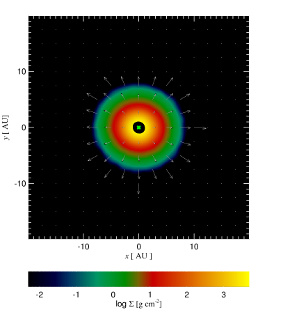
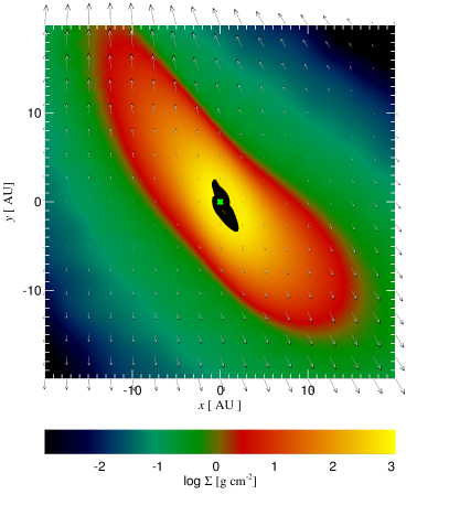
Figure 2: The top view of the gas surface density map for simulation U15 at time t=0.06 (left panel) and $t=0.25$ (right panel). The map is centered on the position of the solid planet (core), which is shown with the thick green symbol. Vectors show the velocity field, also centered on the velocity of the planet. The black dots show locations of individual planetesimals.

Fig. 3 shows the same as Fig. 2, but now at times $t=1$ and $10$ in the left and the right panels, respectively. The figure presents a larger field of view centered onto the star now. The velocity field is also centered onto the star rather than the planet. Note in the left panel that the planetesimals disrupted off the initial gas clump continue to follow orbits similar to that of the densest regions of gas. This is hardly surprising given that potential due to the host clump initially dominates the planetesimals’ orbits (until the host clump is completely disrupted). At late times (see the right panel), the host clump is disrupted into a ring centered about the initial clump’s separation from the star. The planetesimals are also spread into a ring-like feature which shows several streams. The streams appear to have some eccentricity to them. We also note that the fine structure of the streams is now not correlated to the gas component. This is probably caused by the gas gravitational potential being smoothed out due to circularisation of the gas flow, leading to a reduced gas gravitational force on the planetesimals.

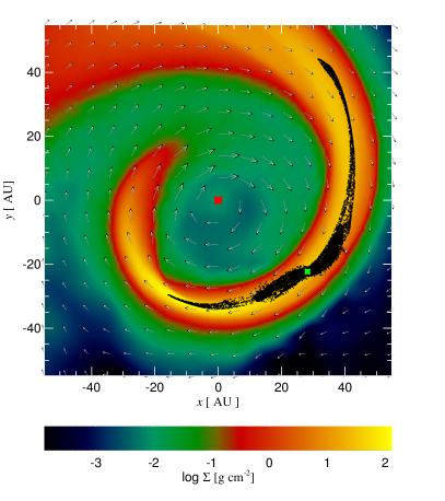
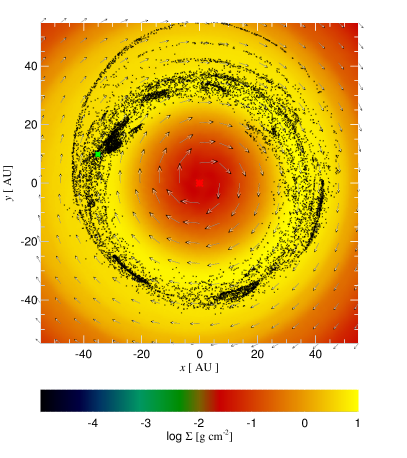
Figure 3: Same as Fig. 2 but at later time; $t=1$ (left panel), and $t=10$ (right panel), except that the center of the coordinate system is now the protostar (the red symbol at the center of the panels). Note that planetesimals initially continue to follow the orbital motion of the densest parts of the gas streams at $t=1$ but separate out at $t=10$ when the gas streams are dispersed and circularised into a ring.

5.2 Simulation U10

As derived in §2.3, the critical injection energy sufficient to inflate the clump to the point of its tidal disruption is $\Delta U_{0}=0.123U_{0}$ for the parameters of the clumps we consider. Therefore, if the approximate theory of §2.3 were correct, the clump would not be disrupted at all in this particular simulation as $\Delta U=0.1U_{0}<\Delta U_{0}$. However, the argument given by equation 6 assumes that the energy injected into the central regions of the gas is shared by the whole clump, so that gas in the clump effectively finds itself on a new (single) polytropic relation. In the simulations, however, the central regions are shifted to a different polytropic relation by the energy injection, whereas the rest of the clump remains at the initial one. One may thus expect the simulation results to differ from the simple analytical prediction.

Figure 4 shows the radial density profile of the host clump (red curve) in simulation U10 at time $t=0.05$ and the theoretical polytropic density profile (black curve) with $n=5/2$ inflated by the energy input from the solid core as assumed in §2.3. One notices significant differences between the two curves, with a tail of gas material extending further out in the red curve. It is this tail that allows some material to siphon out of the Roche lobe and for the gas clump’s radius to continue swelling (cf. equation 2 on this point) as mass is lost.

The left panel of Figure 5 illustrates this initially slow expansion. The host clump is largely intact at $t=3$ in U10. This is in stark contrast to simulation U15 in which the host gas clump was completely obliterated by $t=1$ already (left panel of Fig. 3). However, the host gas clump is eventually destroyed in simulation U10 also. The gas column density and the distribution of planetesimals appear to be quite similar at late times in U10 and U15 ($t=10$, right panels of Figs. 5 and 3, respectively). We shall make a more detailed analysis of planetesimals’ orbits in §6 below.

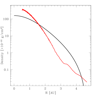
Figure 4: The internal density structure of the expanding protoplanetary clump for simulation U10 ($\Delta U/U_{0}=0.1$) at time $t=0.05$. The red solid line is the actual gas density from the simulation, while the black solid line is a polytrope of 5M_J mass and $4.7$AU radius. The latter curve is expected based on the approximate theory shown in §2.3. The figure shows that a single polytropic relation approximation breaks down after the energy injection, although the approximation is still useful in roughly determining the critical injection energy $\Delta U_{0}$.

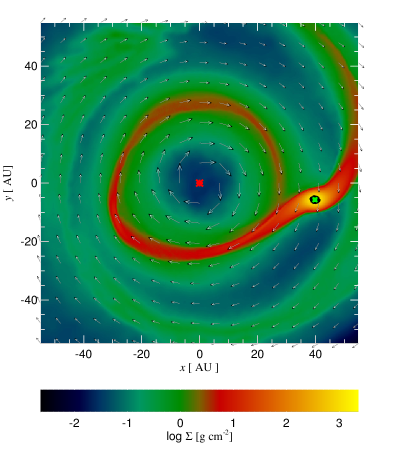
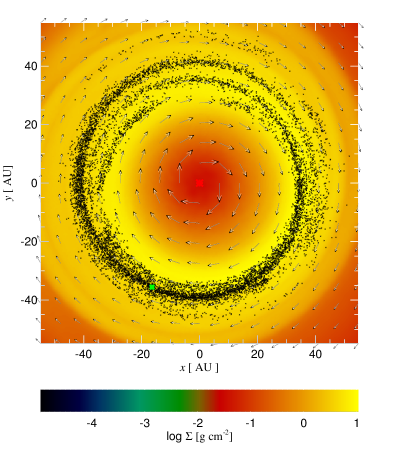
Figure 5: Gas column density projections similar to Fig. 4 but for run U10 at time $t=3$ (left panel) and $t=10$ (right panel). As the planet is less extended than in test U15, the disruption process is much more gradual. At $t=3$ (3 whole orbits of the host clump around the star), only a small fraction of gas mass is lost through the Roche lobe overflow. No planetesimals have yet been unbound from the clump. However, at late time (the right panel), the structure of the disrupted gas and planetesimal population is quite similar to that in U15.

5.3 Simualtion U0

In this simulation, the gas protoplanet is more extended initially, so that $r_{\rm hc}=r_{h}$ at $t=0$. No energy input from the solid core is assumed. Figure 6 shows two snapshots for simulation U0 at times $t=4$ (left panel) and $t=10$ (right panel) in the same format as Fig. 5. The disruption process is not as rapid as in simulation U15 but is a little faster than in U10. The morphology of the gas flow is different: the disrupted gas spiral at $t=4$ is wider in U0 than it is in Fig. 5.

Since the initial disc or planetesimals inside the gas protoplanet is large to begin with ($r_{d}=1$ AU for U0) than for simulations U10 and U15 ($r_{d}=0.4$ AU in both), the flow of disrupted planetesimals is initially wider in U0 (see the banana-shaped feature in the left panel of Fig. 6.) The end result is at least visually not too dissimilar from runs U10 and U15, however.

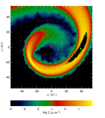
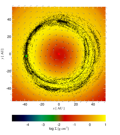
Figure 6: Same as Fig. 5 but for simulation U0, the case where the initial cloud is cooler and already fills its Roche lobe. The corresponding times are $t=4$ (left panel) and $t=10$ (right panel).

6 Orbits of the unbound planetesimals

We now turn to analysis of the unbound population of planetesimals in terms of their orbital elements at the end of the simulations. To avoid confusion, tt must be stressed that, all of our planetesimals remain bound to the central star at the end of the simulations, but some are also bound to the planet, as planetary satellites. The “unbound” population of planetesimals are those particles moving on their own independent heliocentric orbits.

In the simulations, the bound and unbound populations are differentiated according to two conditions. We define the specific energy of a planetesimal with respect to the planet, $E_{\rm rel}$,

$$E_{\rm rel}=-{GM_{p}\over r}+{1\over 2}\;\left(\mathbf{v}-\mathbf{V_{p}}\right)^{2}\;,$$ (26)

where $r$ is the distance between the planet and the planetesimal, $\mathbf{v}$ and $\mathbf{V_{p}}$ are the planetesimal and the planet velocities, respectively (note that these quantities are calculated here at $t=10$ whereas in §2.3 we measured relative positions and velocities of planetesimals and the planet at $t=0$). The planetesimal is considered unbound if

$$E_{\rm rel}>0\;,$$ (27)

and bound if

$$E_{\rm rel}<0\quad{\rm and}\quad r\leq r_{h}^{\prime}\;,$$ (28)

where $r_{h}^{\prime}=R_{0}(M_{p}/3M_{*})^{1/3}$ is the Hill’s radius of the solid planet.

The two populations should be analysed differently, of course. The orbits of the unbound population should be defined with respect to the central star, whereas the orbits of the bound planetesimals are best defined with respect to the planet. In the rest of this section we consider the unbound part of the planetesimals only.

6.1 Simulation U15

Fig. 7 shows the orbital eccentricity (bottom panel) and the inclination (top panel) of the unbound planetesimals versus the semi-major axis of their orbits ($a$) at $t=10$. As explained above, their orbital parameters are calculated with respect to the star as their orbits are heliocentric.

The top panel of figure 7 shows that planetesimals continue to have very small orbital inclinations after the disruption, with the mean inclination angle of only $i\approx 1^{\circ}$. This is natural since in our setup tidal disruption of the host gas protoplanet is symmetric around its orbital plane. In fact, the approximate analytical theory of §2.3 predicts that inclination of planetesimal orbits should remain exactly zero. Therefore, the inclination found in the simulation must result either from a small but finite asymmetry with respect to $z\rightarrow-z$ inversion developing during the disruption, or due to effects not taken into account in the analytical theory.

The central $a\approx 32$ to $a\approx 40$ AU region of this plot shows a higher dispersion in the values of $i$ than do the more distant regions. To understand the origin of this result, we note that the central region is the one where most of the gas ends up after being disrupted, e.g., see the right panel of figure 3. We also note that gas from the disrupted host clump is initially arranged in a high density spiral, gravitational potential of which may well be significant enough to scatter planetesimals about and to pump their inclinations.

This explanation is consistent with the fact that planetesimals on wider orbits, e.g., $a\lower 2.15277pt\hbox{$\;\buildrel>\over{\sim}\;$}42$ AU, which should be affected by the interactions with the gas spiral less, indeed have smaller dispersion in their inclination angles. The non-zero mean value of $i$ for this population, more distant from the planet, should be due to asymmetries developing during the disruption process. Comparison with simulation U0 below, which produces far smaller inclinations, demonstrates that the asymmetries are probably related to the injection of energy in the centre of the host in U15 (and U10). This energy injection increases the entropy of the gas within $r<r_{\rm ej}$ around the planet but not at larger radii. The initial entropy profile is thus strongly unstable to convection in U10 and U15, most likely leading to an asymmetric (with respect to the initial orbital plane of the clump) expansion of the host clump.

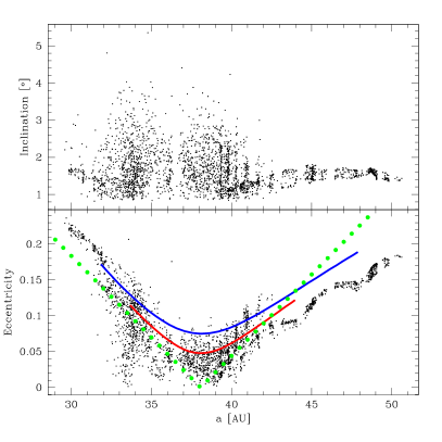
Figure 7: The inclination (top panel) and eccentricity (bottom panel) of the unbound planetesimals versus semi-major axis, $a$, in the simulation U15 at the end of the simulation, $t=10$. Individual planetesimals’ orbital elements are shown with black dots. The coloured chevron-shaped curves are theoretical predictions (see §6.1). The nearly empty vertical contains many planetesimals still bound to the planet, which are not shown here but analysed in §7.

The bottom panel of figure 7 shows the planetesimals in the eccentricity – semi-major axis ($e$–$a$) plane. The coloured curves show the theoretically calculated correlations of $e$ and $a$ with slightly different assumptions (explained below) on the basis of the approximate theory of §3.4. All of these curves were shifted to $a_{0}=38$ AU to fit the simulations better. The shift may be empirically justified as following. Our approximate theory is based on the assumption of an instantaneous disruption of the protoplanet. However, in the simulations the protoplanet is not disrupted instantaneously, and it does migrate inwards during the disruption, presumably due to gas gravitational torques. Therefore, in terms of our approximate theory, the “effective” location of protoplanet disruption should be smaller than the initial radius of the host clump’s circular orbit.

Amongst the theoretically computed curves, the green dots show the simplest one – equation 22. We recall that this equation was obtained with the help of a Taylor decomposition of the specific energy and the specific angular momentum in powers of relatively small parameters $r/R$ and $\delta v/V$. In contrast, the red and the blue curves show the predicted orbits of the planetesimals that did not use the decomposition. To draw the curves, we consider a ring of planetesimals of radius $r=0.3$ and $0.4$ AU for the red and blue curves, respectively. We also assume that the kick velocity of the planetesimals after the disruption, $\mathbf{\Delta v}$ is equal to $\delta\mathbf{v}_{\rm circ}$, where $\delta=0.5$ and $\mathbf{v}_{\rm circ}$ is the circular velocity of the planetesimal before the disruption (cf. equation 8). This simple (but somewhat more accurate than the green dots) theory also predicts the “V” shaped $e-a$ correlation.

We also note that our neglect of the second order terms in equations 13 and 15 lead to the equation 22 being symmetrical with respect to the sign of $a-a_{0}$. The more exact calculations given with the red and the blue curves are not quite symmetrical and also show non-zero eccentricity for all the particles. On the other hand, SPH/N-body simulations show a wider distribution of eccentricities at a given $a$, with some particles reaching $e\approx 0$. Nevertheless, it appears that by varying the parameter $\delta$ (which is only constrained to be less than unity) and by considering the different rings of planetesimals $r$ within the host before its disruption, we can qualitatively explain the observed range of $e$ and $a$ as well as their correlation.

The approximate analytical theory of §3.4 also makes a prediction on the width of the disruption ring, as $w=0.5\zeta$, where $\zeta$ is expected to be of order unity. The debris ring in simulation U15 has width of $\sim 20$ AU, commensurate with $\zeta=1$. The simple “instantaneous” disruption model is thus reasonably accurate in predicting the radial extent of the debris disc in this simulation.

6.2 Unbound debris in U10

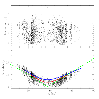
Figure 8: Same as Figure 7 but at the end of simulation U10.

Figure 8 shows the inclination and the eccentricity of the unbound planetesimals in simulation U10, along with theoretical curves, in the same format as in fig. 7. Simulation U10 differs from U15 by the smaller amount of internal energy injected into the host clump by the solid core (planet). As the result, the disruption process is much more gradual and protracted in U10 than in U15 (see §5).

The $e$–$a$ diagram shows a great deal of similarity between simulation U10 and U15, but also some interesting differences. For example, the radial width of the disruption ring is narrower in the former. This makes intuitive sense as there is less internal energy input into the gas clump in U10, and therefore the velocity “kicks” $\Delta v$ after the disruption are probably smaller than they are in U15.

The inclination angle $i$ versus $a$ plot shows somewhat larger mean value and larger dispersion of $i$ in U10 than in U15. In addition, there are pronounced vertical bands in the top panel of Figure 8. Finally, if we break the pattern of fig. 7 on the “gas-dominated” central and the “far-out” population at $a>43$ AU, then its fair to say that in simulation U10 the far-out population is all turned into the central gas-dominated one.

All of these differences are explainable by the fact that the disruption process is more gradual in U10, which means that the tidal tails (arms) of the host clump in the process of disruption (cf. the left panel of fig. 5) survive for longer, before being circularised into a diffuse gaseous ring (the right panel of fig. 5). This implies that the planetesimals are influenced stronger by these tidal tails, explaining a higher dispersion in inclination $i$. In addition to that, the tidal tails “shepherd” the planetesimals out of the cloud, as in seen in the left panels of figures 3 and 6, causing bunching of the orbital parameters in the vertical bands evident in the top panel of figure 8. As the spiral arms survive for longer in U10 than they do in U15, the bunching effect is far stronger in the former than in the latter.

6.3 Unbound planetesimals in simulation U0

Figure 9 shows the orbital parameters of the unbound planetesimals at the end of simulation U0. This figure shows, yet again, the familiar $e$–$a$ correlation diagram but a significantly different distribution of planetesimal orbital inclinations. The red and the blue curves in this case were computed assuming two rings of planetesimals with $r=0.75$ and $1$ AU, respectively, because the planetesimal disc is larger in U0 than in U10 and U15, and we used $\delta=0.9$ (see §6.1). The latter is chosen by trial and error to find a visually reasonable match to the distribution of orbits in the simulation.

The much stronger bunching of planetesimals towards the $i=0$ plane is a testament to the different nature of the host clump disruption in U0 as compared to U10 and U15. While in the latter two the inner region of the clump was the actual source of the disruption (as the core accretion energy was dumped there), in U0 the innermost region is “passive”. Therefore the disruption process, as experienced by the planetesimals initially located at $r\leq 1$ AU for this simulation, is much less abrupt, leading to even less inclined orbits for the unbound particles. In addition, as mentioned in 6.1, the injection of energy stirs up strong convective motions in those simulations, pumping up asymmetries and thus orbital inclinations.

On the other hand, the larger dispersion in values of $i$ in the centre of the planetesimal ring, and the presence of the vertical bands in fig. 9 confirms that these features are formed by the tidal arms (tails) of the host clump before they are wound up and completely erased.

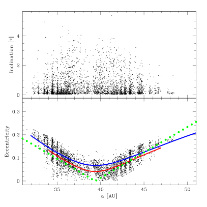
Figure 9: Same as Figs. 7 and 8, except for the red and blue curves, as explained in the text (see §6.3). Note the much larger $i\approx 0$ population of planetesimals in this simulation compared to U10 and U15

7 Bound population: planet satellites

We now switch to discussing planetesimals bound to the solid planet, e.g., those that have a negative energy with respect to the planet and that are within the planet’s Hill’s radius (see §6).

Figure 10 presents the orbital parameters of the planetesimal orbits around the planet for the simulation U15 (left panel) and U10 (right panel). The red vertical lines show the location of the planet’s influence radius, $r_{i}$, defined by equation 9. This radius divides the region where gravitational potential is dominated by the solid planet (inside $r_{i}$) and the gas (outside $r_{i}$). As stated in §3.3, the orbits of planetesimals are expected to be only mildly perturbed within $r_{i}$ and suffer strong perturbations outside $r_{i}$, in fact being completely unbound from the planet at $r\gg r_{i}$.

Figure 10 confirms this expectation qualitatively, including the fact that there are very few particles with semi-major axis $a$ larger than 0.4 AU. The particles inside $r_{i}$ tend to have mild eccentricity $0\leq e\leq 0.4$, whereas planetesimals outside $r_{i}$ have higher values of $e$ on average. The orbital inclination $i$ also increases with $a$, reaching $10^{\circ}$ to $20^{\circ}$ outside $r_{i}$ in simulation U15, and slightly higher values in U10. Note that a larger mean value of $i$ in U10 compared to that in U15 found here for the bound population is consistent with a similar trend that we found for the unbound population (cf. figures 7 and 8).

Figure 11 shows the orbital parameters of the bound population of planetesimals in simulation U0. There is a marked difference in these distributions compared with that for U15 and U10. Instead of a monotonic increase in eccentricities and inclinations with increasing $a$, evident in Figure 10, here there is an almost a step-function change in the nature of the orbits. Orbits at $a\lower 2.15277pt\hbox{$\;\buildrel<\over{\sim}\;$}0.3$ have small eccentricity, $0\leq e\leq 0.2$, whereas orbits at $a\lower 2.15277pt\hbox{$\;\buildrel>\over{\sim}\;$}0.3$ have a large spread in eccentricities, with some approaching unity. The planetesimals with the largest values of $e$ may become unbound later since their orbits are comparable to $r_{h}$. There is also a group of particles with large inclinations, $i\lower 2.15277pt\hbox{$\;\buildrel>\over{\sim}\;$}90^{\circ}$ at $a\approx 0.35$ AU.

The significant differences in the orbits of the bound populations of planetesimals between Figures 10 and 11 demonstrate that the exact way in which the innermost region of the host clump is disrupted influences the orbits of the “satellites” remaining after the disruption. By extension it also means that the results would also be somewhat different if there was a massive gas atmosphere around the solid protoplanetary core.

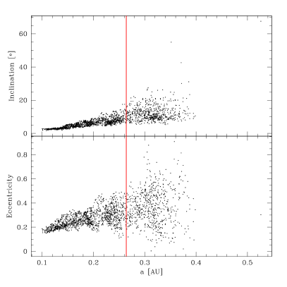
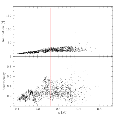
Figure 10: The bound population of planetesimals around the solid core (planet). The orbital characteristic are calculated with respect to the planet rather than the star. Left: Simulation U15, Right: simulation U10.

Figure 11: Same as Fig. 10 but for simulation U0.

8 Discussion

8.1 General conclusions

In this paper we considered the predictions of the TD hypothesis for the “planetesimal” debris left over after the disruption of a single gas host clump. These gas clumps are the parent bodies within which all (or at least most) of planet formation action takes place in the TD hypothesis. The most important results of our paper can be summarised as following:

1. In the context of TD hypothesis, large solids form only inside the massive gas host clumps (because the densities of solids initially reflect that of gas, and gas densities are orders of magnitude higher inside the host clumps than in the “ambient disc”; see, e.g., Nayakshin, 2011a; Cha & Nayakshin, 2011) that are then disrupted. The solid debris is then spread around in a ring around the disruption location. TD hypothesis thus generically predicts rings of planetesimals remaining after planet formation rather than continuous discs.

2. The role of planetesimals in the formation of planets may be very different in the CA and TD scenarios. Whereas planets could not have formed without planetesimals forming first in the CA picture, in the TD hypothesis this is less clear. In the latter case, once the initial proto solid core is born by gravitational collapse of the grain-dominated inner region of the host clump(Nayakshin, 2010b, 2011a), further growth may be dominated by the proto solid core accreting $\sim$ cm to tens of cm grains. Solids in this size range experience aerodynamic drag that is strong enough to dump possible centrifugal support and yet small enough to sediment to the centre of the host clump within its lifetime (see Fig. 1). Bodies in the planetesimal size range, i.e., km-sized and larger, on the other hand, experience too weak an aerodynamic drag. They are not expected to join the solid core en masse if they have some orbital support due to an excess angular momentum or chaotic convective motions of the gas in the centre of the host clump. In this case planetesimals are no parent bodies of planets in the strict sense.

On the other hand, if turbulence, convection or angular momentum prevents small grains from reaching the proto solid core directly, turning most of these grains into planetesimals as discussed in §3.2, then the situation is less clear. If this happens sufficiently close to the proto solid core and planetesimal densities are high, most of that material can be subsequently accreted by the proto core somewhat like in the CA theory. In this case planetesimals are also building blocks of planets, with only those on larger less bound orbits managing to avoid being accreted onto the core.

3. Related to the point above, the solid planetary cores and the planetesimal debris form at approximately same time in our picture. After host gas clump disruption, some of the solid debris around the planetary core could fall on it and be accreted in direct collisions, so that planetary growth could actually continue in a manner analogous to that of the later oligarchic stages of solid core assembly in the traditional scenario (e.g., Safronov, 1972). In particular, as velocity dispersion of the disrupted population is high, e.g. a fraction of a km s^-1, only large planetesimals of size $\lower 2.15277pt\hbox{$\;\buildrel>\over{\sim}\;$}1000$ km would continue their growth, whereas smaller objects would accrete on large bodies or fragment in collisions with smaller bodies. If they fragment to sizes as small as a few metres then their inward radial migration inside the gas disc becomes important.

4. Also related to point (2) above, the mass budget of planetesimals can be potentially very different in the two planet formation theories. In the CA scenario, the initial population of planetesimals must have had a total mass larger than the total high-Z element (other than H and He) mass of the resulting planets. This does not have to be the case in the TD scenario. In particular, there does not seem anything wrong with assuming that the debris population may be far less massive than the protoplanetary core.

5. In the CA scenario, the properties of the protoplanetary disc are expected to be a rather smoothly varying function of radius, except for the regions near the ice line (e.g., Armitage, 2010). Thus one expects that planetesimal properties are also a smoothly varying function of $R$. In contrast, in the TD hypothesis, it is the host clump that determines the outcome of the planet formation process. The internal structure of the clump is a strong function of its mass (Nayakshin, 2010b, 2011a); that structure is non-uniquely coupled to radius $R$ where the clump is disrupted. It is possible that clumps of different history, mass, internal structure are disrupted at roughly same location. Further, we envisage a number of host clumps forming and being destroyed during the early gas-rich phase as required to explain the FU Ori outbursts of young protostars (Nayakshin & Lodato, 2011). This implies a far greater diversity in the properties of the solid debris at the same spatial location than is possible in the CA model.

6. We found in this paper that disruption of a host gas clump generically produces a “V”-shaped pattern in the eccentricity-semi-major axis space for the planetesimal population released by the disruption. The planetesimals in the centre of the pattern have nearly circular orbits while whose at the edges of it are much more eccentric. The maximum eccentricities possible can be estimated based on the simple analytical theory; from equations 22 to 25, it follows that, within a factor of $\sim 2$, it is $e_{\rm max}\sim r_{h}/R\approx 0.2$ for host clump mass of $\sim 10$ Jupiter masses.

7. The eccentricities and inclinations of the disrupted planetesimal population are generally much too high to allow planetesimals to stick to one another. The typical dispersion velocity of the disrupted population is $\delta v\sim v_{K}r_{h}/R\sim 0.1v_{K}$. At the distance of the Kuiper belt, for example, this yields dispersion velocity of the order of $300$ m/s. Only Pluto-sized bodies could survive equal-size collisions at these velocities. Accretion on massive solid cores, however, is allowed as already noted in (3) above, so the post-disruption evolution may be somewhat similar to the final phases of the run-away growth of planetary embryos in the traditional scenario (e.g., Safronov, 1972).

8. We also find that solid bodies on orbits tightly bound to the planetary core could survive the disruption of the gas host clump, remaining bound to the planet. These bodies are satellites of the planetary cores. Satellites on orbits more strongly bound to the planet are affected by the gas envelope destruction less than those on less bound orbits. Some of the outermost satellites may even find themselves in eccentric counter-rotating orbits (e.g., see fig. 10). This is qualitatively similar to the satellites of the giant planets in the Solar System, although we note that our simulations are not designed to study these issues; one also would need to model composition, size differences and long-term survivability of the bound objects.

8.2 Potential relevance to the Solar System

Even though we did not specifically attempt to reproduce the structure of the outer Solar System here (which would require an additional study of how the system evolves on the 4.5 Giga year time scale), our simulations do have potentially interesting implications for it. We mention these implications only briefly here, with the intent of quantifying them in a future publication:

• One of the key properties of the trans-Neptunian region of the Solar System, including the Kuiper belt, is the “mass deficit problem”. The current mass of the Kuiper belt is estimated at $\sim 0.01-0.1{\,{\rm M}_{\oplus}}$ (Bernstein et al., 2004). On the other hand, to grow the observed populations of solid bodies in the context of the Safronov (1972) model for formation of solids, 10 to 100 ${\,{\rm M}_{\oplus}}$ of solids is required (e.g., Kenyon & Luu, 1999). Thus, removal of $\lower 2.15277pt\hbox{$\;\buildrel>\over{\sim}\;$}99.9$% of solid material is required. In the TD hypothesis, solids are made within the central fractions of AU of the host gas clumps (Nayakshin, 2010b). The host clumps contain as much as $\sim 60{\,{\rm M}_{\oplus}}$ of high-Z elements (Nayakshin, 2011a) which are then partially used to make the massive solid cores, the “planetesimals”, and partially remain bound to gas in small grains. If it is possible to build solid cores as massive as $\sim 10{\,{\rm M}_{\oplus}}$ by direct gravitational collapse and accretion of $\sim$cm size grains (Nayakshin, 2011a), it should also be possible to build Pluto-sized objects without having to put tens of ${\,{\rm M}_{\oplus}}$ of material into the planetesimals. There is thus no mass deficit problem for the Kuiper belt in the TD scenario.

• There is a sharp outer edge to the Kuiper belt at around $R\approx 50$ AU which is currently not well understood (e.g., Morbidelli et al., 2008). The disruption of a gas host clump naturally produces a ring with sharp outer and inner edges (point 1 above) because the range of orbits available to planetesimals after disruption is limited by the parameters of the initial host clump. This could naturally account for the outer edge of the Kuiper belt objects.

• The structure of the classical Kuiper belt is best explained by our model if we assume that the left hand side (lower $a$) of the disruption ring (e.g., Fig. 9) has been destroyed by interactions with planets. Realistically, the planet, left at $a\sim 35-39$ AU at the end of our simulations, could have continued to migrate inward via type I migration in the gas disc: the disrupted gas ring is still quite massive (5 Jupiter masses for our simulations here, and there would be more at larger $R$ to effect the migration of the host clump in the first place). Using the standard type-I gas migration (e.g., Tanaka et al., 2002) for Neptune initially located at $\approx 40$ AU, assuming the disc mass being $\sim 10$ Jupiter masses, and the gas disc aspect ratio of $H/R\sim 0.1$ yields type I migration rate time scale of $\sim 10^{6}$ yrs. This is sufficiently fast to allow Neptune to migrate inward significantly to end up, for example, in the configuration proposed by the NICE model of the outer Solar System (Gomes et al., 2005). While migrating inward in the gas disc, Neptune would have scattered the left part of the “V”-pattern of the planetesimals, but leaving behind the right hand side of the pattern as a belt reminiscent of the Kuiper belt.

• Kuiper belt contains the hot and the cold populations. These are best accounted for by two different gas clump disruptions in our model. The hot population in our model would have most naturally resulted if the host gas protoplanet rotation axis were highly inclined to the orbital plane. In this case one could end up with higher inclinations than we obtained here.

• Nesvorný et al. (2010) show that if planetesimals form by a local gravitational collapse in a high density environment, then one can naturally explain the surprisingly large fraction of binaries in the $\sim$100 km class low-inclination objects in the classical Kuiper Belt. We note that our model produces “planetesimals” in a similar fashion (gravitational collapse in a high density environment) albeit inside of the host clumps rather than the disc. Therefore by extension one might expect to see a high fraction of massive objects locked in binaries after the dissipation of the host clump. This idea however needs to be checked with a longer time $N$-body calculation as there are non trivial physical constraints on collisional destruction of binaries in the Kuiper Belt (Nesvorný et al., 2011).

9 Conclusions

We have considered the origin of solid debris, such as comets, asteroids and large bodies such as Pluto in the context of a recent planet formation hypothesis (Tidal Downsizing). We assumed (see §3.2) that the solid “debris” is formed in a way very similar to the massive solid protoplanetary cores themselves, e.g., inside the $\sim 10$ Jupiter mass host gas clouds. The latter are eventually disrupted either tidally or due to an internal energy release during the solid core accretion. The release of these solid bodies into the field forms rings potentially reminiscent of the Kuiper belt and the debris discs around nearby main sequence stars. While much work remains to be done to detail predictions of the TD hypothesis further, it is already clear that these predictions are sufficiently different from the standard planetesimal-based paradigm for planet formation (Safronov, 1972) to be critically tested by observations in the near future.

As an astrophysical aside, we note that the rapid accretion of large solid bodies (Pluto-like and even Neptune-like) in the TD scheme suggests that planet and solid debris formation is a very robust process and may even occur in very crowded environments such as the inner parsecs of galaxies (Nayakshin et al., 2012; Zubovas et al., 2011); this is an untenable proposition in the CA model.

References

- Alibert et al. (2005) Alibert Y., Mordasini C., Benz W., Winisdoerffer C., 2005, A&A, 434, 343
- Armitage (2010) Armitage P. J., 2010, Astrophysics of Planet Formation
- Aumann et al. (1984) Aumann H. H., Beichman C. A., Gillett F. C., de Jong T., Houck J. R., Low F. J., Neugebauer G., Walker R. G., Wesselius P. R., 1984, ApJL, 278, L23
- Baruteau et al. (2011) Baruteau C., Meru F., Paardekooper S.-J., 2011, MNRAS, 416, 1971
- Bernstein et al. (2004) Bernstein G. M., Trilling D. E., Allen R. L., Brown M. E., Holman M., Malhotra R., 2004, AJ, 128, 1364
- Boley et al. (2007) Boley A. C., Hartquist T. W., Durisen R. H., Michael S., 2007, ApJL, 656, L89
- Boley et al. (2010) Boley A. C., Hayfield T., Mayer L., Durisen R. H., 2010, Icarus, 207, 509
- Boley et al. (2011) Boley A. C., Helled R., Payne M. J., 2011, ArXiv e-prints
- Boss (1997) Boss A. P., 1997, Science, 276, 1836
- Boss (1998) Boss A. P., 1998, ApJ, 503, 923
- Bottke et al. (2005) Bottke W. F., Durda D. D., Nesvorný D., Jedicke R., Morbidelli A., Vokrouhlický D., Levison H., 2005, ICARUS, 175, 111
- Cha & Nayakshin (2011) Cha S.-H., Nayakshin S., 2011, MNRAS, 415, 3319
- Cuzzi et al. (2008) Cuzzi J. N., Hogan R. C., Shariff K., 2008, ApJ, 687, 1432
- Donnison & Williams (1975) Donnison J. R., Williams I. P., 1975, MNRAS, 172, 257
- Dunham & Vorobyov (2012) Dunham M. M., Vorobyov E. I., 2012, ApJ, 747, 52
- Forgan & Rice (2011) Forgan D., Rice K., 2011, MNRAS, 417, 1928
- Gingold & Monaghan (1977) Gingold R. A., Monaghan J. J., 1977, MNRAS, 181, 375
- Goldreich & Ward (1973) Goldreich P., Ward W. R., 1973, ApJ, 183, 1051
- Gomes et al. (2005) Gomes R., Levison H. F., Tsiganis K., Morbidelli A., 2005, Nature, 435, 466
- Helled & Schubert (2008) Helled R., Schubert G., 2008, Icarus, 198, 156
- Hellyer (1970) Hellyer B., 1970, MNRAS, 148, 383
- Ida & Lin (2008) Ida S., Lin D. N. C., 2008, ApJ, 685, 584
- Ida & Lin (2010) Ida S., Lin D. N. C., 2010, ApJ, 719, 810
- Ilee et al. (2011) Ilee J. D., Boley A. C., Caselli P., Durisen R. H., Hartquist T. W., Rawlings J. M. C., 2011, MNRAS, 417, 2950
- Johansen et al. (2007) Johansen A., Oishi J. S., Low M., Klahr H., Henning T., Youdin A., 2007, Nature, 448, 1022
- Kenyon & Luu (1999) Kenyon S. J., Luu J. X., 1999, AJ, 118, 1101
- Larson (1969) Larson R. B., 1969, MNRAS, 145, 271
- Lucy (1977) Lucy L. B., 1977, AJ, 82, 1013
- Machida et al. (2011) Machida M. N., Inutsuka S.-i., Matsumoto T., 2011, ApJ, 729, 42
- Mayer et al. (2004) Mayer L., Quinn T., Wadsley J., Stadel J., 2004, ApJ, 609, 1045
- McCrea & Williams (1965) McCrea W. H., Williams I. P., 1965, Royal Society of London Proceedings Series A, 287, 143
- Michael et al. (2011) Michael S., Durisen R. H., Boley A. C., 2011, ApJL, 737, L42+
- Mizuno (1980) Mizuno H., 1980, Progress of Theoretical Physics, 64, 544
- Monaghan (1992) Monaghan J. J., 1992, ARA&A, 30, 543
- Morbidelli et al. (2008) Morbidelli A., Levison H. F., Gomes R., 2008, The Dynamical Structure of the Kuiper Belt and Its Primordial Origin. pp 275–292
- Nayakshin (2010a) Nayakshin S., 2010a, MNRAS, 408, L36
- Nayakshin (2010b) Nayakshin S., 2010b, MNRAS, 408, 2381
- Nayakshin (2011a) Nayakshin S., 2011a, MNRAS, 413, 1462
- Nayakshin (2011b) Nayakshin S., 2011b, MNRAS, 416, 2974
- Nayakshin (2011c) Nayakshin S., 2011c, MNRAS, 410, L1
- Nayakshin et al. (2011) Nayakshin S., Cha S.-H., Bridges J. C., 2011, MNRAS, 416, L50
- Nayakshin & Lodato (2011) Nayakshin S., Lodato G., 2011, ArXiv e-prints
- Nayakshin et al. (2012) Nayakshin S., Sazonov S., Sunyaev R., 2012, MNRAS, 419, 1238
- Nesvorný et al. (2003) Nesvorný D., Bottke W. F., Levison H. F., Dones L., 2003, ApJ, 591, 486
- Nesvorný et al. (2010) Nesvorný D., Jenniskens P., Levison H. F., Bottke W. F., Vokrouhlický D., Gounelle M., 2010, ApJ, 713, 816
- Nesvorný et al. (2011) Nesvorný D., Vokrouhlický D., Bottke W. F., Noll K., Levison H. F., 2011, AJ, 141, 159
- Nesvorný et al. (2010) Nesvorný D., Youdin A. N., Richardson D. C., 2010, AJ, 140, 785
- Perri & Cameron (1974) Perri F., Cameron A. G. W., 1974, ICARUS, 22, 416
- Pollack et al. (1996) Pollack J. B., Hubickyj O., Bodenheimer P., Lissauer J. J., Podolak M., Greenzweig Y., 1996, Icarus, 124, 62
- Rafikov (2005) Rafikov R. R., 2005, ApJL, 621, L69
- Rafikov (2006) Rafikov R. R., 2006, ApJ, 648, 666
- Rafikov (2011) Rafikov R. R., 2011, ApJ, 727, 86
- Rees (1976) Rees M. J., 1976, MNRAS, 176, 483
- Rice et al. (2005) Rice W. K. M., Lodato G., Armitage P. J., 2005, MNRAS, 364, L56
- Safronov (1972) Safronov V. S., 1972, Evolution of the protoplanetary cloud and formation of the earth and planets.. Jerusalem (Israel): Israel Program for Scientific Translations, Keter Publishing House, 212 p.
- Shapiro & Teukolsky (1983) Shapiro S. L., Teukolsky S. A., 1983, Black holes, white dwarfs, and neutron stars: The physics of compact objects
- Springel (2005) Springel V., 2005, MNRAS, 364, 1105
- Springel (2010) Springel V., 2010, ARA&A, 48, 391
- Stevenson (1982) Stevenson D. J., 1982, P&SS, 30, 755
- Stewart & Leinhardt (2009) Stewart S. T., Leinhardt Z. M., 2009, ApJL, 691, L133
- Tanaka et al. (2002) Tanaka H., Takeuchi T., Ward W. R., 2002, ApJ, 565, 1257
- Vorobyov (2011) Vorobyov E. I., 2011, ApJL, 728, L45+
- Vorobyov & Basu (2005) Vorobyov E. I., Basu S., 2005, ApJL, 633, L137
- Vorobyov & Basu (2006) Vorobyov E. I., Basu S., 2006, ApJ, 650, 956
- Weidenschilling (1977) Weidenschilling S. J., 1977, MNRAS, 180, 57
- Wyatt (2008) Wyatt M. C., 2008, ARA&A, 46, 339
- Wyatt et al. (2007) Wyatt M. C., Smith R., Greaves J. S., Beichman C. A., Bryden G., Lisse C. M., 2007, ApJ, 658, 569
- Wyatt et al. (2007) Wyatt M. C., Smith R., Su K. Y. L., Rieke G. H., Greaves J. S., Beichman C. A., Bryden G., 2007, ApJ, 663, 365
- Youdin & Goodman (2005) Youdin A. N., Goodman J., 2005, ApJ, 620, 459
- Youdin & Shu (2002) Youdin A. N., Shu F. H., 2002, ApJ, 580, 494
- Zubovas et al. (2011) Zubovas K., Nayakshin S., Markoff S., 2011, ArXiv e-prints
- Zuckerman (2001) Zuckerman B., 2001, ARA&A, 39, 549