Scattering and bound states of spin-0 particles in a nonminimal vector double-step potential

Abstract

The problem of spin-0 particles subject to a nonminimal vector double-step potential is explored in the context of the Duffin-Kemmer-Petiau theory. Surprisingly, one can never have an incident wave totally reflected and the transmission amplitude has complex poles corresponding to bound states. The interesting special case of bosons embedded in a sign potential with its unique bound-state solution is analyzed as a limiting case.







Keywords: DKP equation, nonminimal coupling, double-step potential

PACS Numbers: 03.65.Ge, 03.65.Pm

1 Introduction

The first-order Duffin-Kemmer-Petiau (DKP) equation [1]-[4] is often seen as an alternative and rather unusual form for describing spin-0 and spin-1 particles. Although the second-order and the DKP formalisms are equivalent in the case of minimally coupled vector interactions [5]-[7], the last formalism opens news horizons as far as it allows the inclusion of other kinds of couplings in a straightforward way [8]-[9]. The nonminimal vector interaction, for instance, refers to a kind of charge-conjugate invariant coupling which behaves like a vector under a Lorentz transformation. The invariance of the nonminimal vector potential under charge conjugation means that it does not couple to the charge of the boson and so it does not distinguish particles from antiparticles. Hence, whether one considers spin-0 or spin-1 bosons, this sort of interaction can not exhibit Klein’s paradox [10]. Nonminimal vector interactions, added by other kinds of Lorentz structures, have already been used successfully in a phenomenological context for describing the scattering of mesons by nuclei [11]-[18]. Nonminimal vector couplings with diverse functional forms for the potential functions have been explored in the literature [10], [19]-[27].

In the present work some aspects of the stationary states of spin-0 bosons in a double-step potential with a nonminimal vector coupling are analyzed. Scattering states are analyzed and an oscillatory transmission coefficient is found. An interesting point is that the transmission coefficient never vanishes, regardless the size of the potential barrier. In sharp contrast with a nonrelativistic scheme, the transmission amplitude exhibits complex poles corresponding to bound-state solutions for a potential of sufficient intensity. The eigenenergies for bound states are solutions of transcendental equations classified as eigenvalues of the parity operator. Those intriguing results are interpreted in terms of solutions of an effective Schrödinger equation for a finite square well with additional $\delta$-functions situated at the borders. The case of a sign potential (interpreted as a shifted $\delta$-function potential) with its unique bound-state solution is analyzed as a limiting case of the double-step potential.

2 The nonminimal vector double-step potential

The DKP equation for a free boson is given by [4] (with units in which $\hbar=c=1$)

$$\left(i\beta^{\mu}\partial_{\mu}-m\right)\psi=0$$ (1)

where the matrices $\beta^{\mu}$ satisfy the algebra $\beta^{\mu}\beta^{\nu}\beta^{\lambda}+\beta^{\lambda}\beta^{\nu}\beta^{\mu}=g^{\mu\nu}\beta^{\lambda}+g^{\lambda\nu}\beta^{\mu}$ and the metric tensor is $g^{\mu\nu}=\,$diag$\,(1,-1,-1,-1)$. That algebra generates a set of 126 independent matrices whose irreducible representations are a trivial representation, a five-dimensional representation describing the spin-0 particles and a ten-dimensional representation associated to spin-1 particles. The second-order Klein-Gordon and Proca equations are obtained when one selects the spin-0 and spin-1 sectors of the DKP theory. A well-known conserved four-current is given by $J^{\mu}=\bar{\psi}\beta^{\mu}\psi$$/2$ where the adjoint spinor $\bar{\psi}$ is given by $\bar{\psi}=\psi^{\dagger}\eta^{0}$ with $\eta^{0}=2\beta^{0}\beta^{0}-1$. The time component of this current is not positive definite but it may be interpreted as a charge density. Then the normalization condition $\int d\tau\,J^{0}=\pm 1$ can be expressed as $\int d\tau\,\bar{\psi}\beta^{0}\psi=\pm 2$, where the plus (minus) sign must be used for a positive (negative) charge.

With the introduction of nonminimal vector interactions, the DKP equation can be written as [8]

$$\left(i\beta^{\mu}\partial_{\mu}-m-i[P,\beta^{\mu}]A_{\mu}\right)\psi=0$$ (2)

where $P$ is a projection operator ($P^{2}=P$ and $P^{\dagger}=P$) in such a way that $\bar{\psi}[P,\beta^{\mu}]\psi$ behaves like a vector under a Lorentz transformation as does $\bar{\psi}\beta^{\mu}\psi$. Once again $\partial_{\mu}J^{\mu}=0$ [10]. If the potential is time-independent one can write $\psi(\vec{r},t)=\phi(\vec{r})\exp(-iEt)$, where $E$ is the energy of the boson, in such a way that the time-independent DKP equation becomes

$$\left[\beta^{0}E+i\beta^{i}\partial_{i}-\left(m+i[P,\beta^{\mu}]A_{\mu}\right)\right]\phi=0$$ (3)

For the case of spin 0, we use the representation for the $\beta^{\mu}$ matrices given by [28]

$$\beta^{0}=\begin{pmatrix}\theta&\overline{0}\\ \overline{0}^{T}&\mathbf{0}\end{pmatrix},\quad\beta^{i}=\begin{pmatrix}\widetilde{0}&\rho_{i}\\ -\rho_{i}^{T}&\mathbf{0}\end{pmatrix},\quad i=1,2,3$$ (4)

where

$$\ \theta = \begin{pmatrix}0&1\\ 1&0\end{pmatrix},\quad\rho_{1}=\begin{pmatrix}-1&0&0\\ 0&0&0\end{pmatrix}$$

$$\rho_{2} = \begin{pmatrix}0&-1&0\\ 0&0&0\end{pmatrix},\quad\rho_{3}=\begin{pmatrix}0&0&-1\\ 0&0&0\end{pmatrix}$$

$\overline{0}$, $\widetilde{0}$ and $\mathbf{0}$ are 2$\times$3, 2$\times$2 and 3$\times$3 zero matrices, respectively, while the superscript T designates matrix transposition. Here the projection operator can be written as [8] $P=\left(\beta^{\mu}\beta_{\mu}-1\right)/3=\mathrm{diag}\,(1,0,0,0,0)$. In this case $P$ picks out the first component of the DKP spinor. The five-component spinor can be written as $\psi^{T}=\left(\psi_{1},...,\psi_{5}\right)$ in such a way that the time-independent DKP equation for a boson constrained to move along the $X$-axis, restricting ourselves to potentials depending only on $x$, decomposes into

$$\left(\frac{d^{2}}{dx^{2}}+E^{2}-m^{2}+A_{0}^{2}-A_{1}^{2}+\frac{dA_{1}}{dx}\right)\phi_{1}=0$$

$$\phi_{2}=\frac{1}{m}\left(E+iA_{0}\right)\,\phi_{1}$$ (6)

$$\phi_{3}=\frac{i}{m}\left(\frac{d}{dx}+A_{1}\right)\phi_{1},\quad\phi_{4}=\phi_{5}=0$$

Meanwhile,

$$J^{0}=\frac{E}{m}\,|\phi_{1}|^{2},\quad J^{1}=\frac{1}{m}\text{Im}\left(\phi_{1}^{\ast}\,\frac{d\phi_{1}}{dx}\right)$$ (7)

Given that the interaction potentials satisfy certain conditions, we have a well-defined Sturm-Liouville problem for determining the possible discrete or continuous eigenvalues of the system. We also note that there is only one independent component  of the DKP spinor for the spin-0 sector. It is not hard to see that the spectrum is symmetrical about $E=0$, as it should be since $A_{\mu}$ does not distinguish particles from antiparticles. Note also that for ensuring the covariance of the DKP theory under the parity operation one must have $A_{0}\left(-x\right)=+A_{0}\left(x\right)$ and $A_{1}\left(-x\right)=-A_{1}\left(x\right)$. It follows that the parity of $\phi_{3}$ is opposite to that one of $\phi_{1}$ and $\phi_{2}$ in such a way that the DKP spinor has a definite parity. Furthermore, the change $A_{\mu}\rightarrow A_{\mu}+constant$ drastically changes the spectrum.

Let us focus our attention on the space component of a nonminimal potential with $A_{1}\left(-x\right)=-A_{1}\left(x\right)$. We consider the double-step potential

$$A_{1}\left(x\right)=V_{0}\left[\theta\left(x-a\right)-\theta\left(-x-a\right)\right]$$ (8)

with $V_{0}$ and $a$ defined to be real numbers ($a>0$) and $\theta\left(x\right)$ is the Heaviside step function. It is of interest to note that in the limit $a\rightarrow 0$, the double-step function reduces to $V_{0}\,$sgn$\left(x\right)$, where  sgn$\left(x\right)=x/|x|$. Our problem is to solve (6) for $\phi_{1}$ and to determine the allowed energies. In this case the first line of (6) can be written as

$$\frac{d^{2}\phi_{1}}{dx^{2}}+\left\{E^{2}-m^{2}+V_{0}\left[\delta\left(x-a\right)+\delta\left(x+a\right)\right]\right.$$

$$\qquad\qquad\qquad\qquad\qquad\qquad\qquad\left.-V_{0}^{2}\left[\theta\left(x-a\right)+\theta\left(-x-a\right)\right]\right\}\phi_{1}=0$$ (9)

where $\delta\left(x\right)=d\theta\left(x\right)/dx$ is the Dirac delta function. We turn our attention to scattering states so that the solutions describing spinless bosons coming from the left can be written as

$$\phi_{1}(x)=\left\{\begin{array}[]{cc}Ae^{+i\eta\frac{x}{a}}+Be^{-i\eta\frac{x}{a}}&\text{{for }}x<-a\\ &\\ Ce^{+i\xi\frac{x}{a}}+De^{-i\xi\frac{x}{a}}&\text{{for }}|x|<a\\ &\\ Fe^{+i\eta\frac{x}{a}}&\text{{for }}x>a\end{array}\right.$$ (10)

where

$$\xi=a\sqrt{E^{2}-m^{2}},\quad\eta=\sqrt{\xi^{2}-\mathcal{\upsilon}^{2}},\quad\mathcal{\upsilon}=aV_{0}$$ (11)

Then, $\phi_{1}$ describes an incident wave moving to the right ($\eta$ is a real number) and a reflected wave moving to the left with

$$J^{1}\left(x<-a\right)=\frac{\eta}{am}\left(|A|^{2}-|B|^{2}\right)$$ (12)

and a transmitted wave moving to the right with

$$J^{1}\left(x>a\right)=\frac{\eta}{am}|F|^{2}$$ (13)

We demand that $\phi_{1}$ be continuous at $x=\pm a$, i. e.

$$\lim_{\varepsilon\rightarrow 0}\left.\phi_{1}\right|_{x=\pm a-\varepsilon}^{x=\pm a+\varepsilon}=0$$ (14)

Otherwise, (9) would contain the derivative of a $\delta$-function. Effects due to the potential on $d\phi_{1}/dx$ in the neighbourhood of $\ x=\pm a$ can be evaluated by integrating (9) from $\pm a-\varepsilon$ to $\pm a+\varepsilon$ and taking the limit $\varepsilon\rightarrow 0$. The connection formula between $d\phi_{1}/dx$ at the right and $d\phi_{1}/dx$ at the left can be summarized as

$$\lim_{\varepsilon\rightarrow 0}\left.\frac{d\phi_{1}}{dx}\right|_{x=\pm a-\varepsilon}^{x=\pm a+\varepsilon}=-\frac{\mathcal{\upsilon}}{a}\,\phi_{1}(\pm a)$$ (15)

With $\phi_{1}$ given by (10), conditions (14) and (15) imply that

$$e^{i\eta}F = e^{i\xi}C+e^{-i\xi}D$$

$$e^{-i\eta}A+e^{i\eta}B = e^{-i\xi}C+e^{i\xi}D$$

$$e^{i\eta}F\left(\eta-i\mathcal{\upsilon}\right) = \xi\left(e^{i\xi}C-e^{-i\xi}D\right)$$

$$\xi\left(e^{-i\xi}C-e^{i\xi}D\right) = \left(\eta+i\mathcal{\upsilon}\right)e^{-i\eta}A-\left(\eta-i\mathcal{\upsilon}\right)e^{i\eta}B$$

Omitting the algebraic details, we state the solution for the relative amplitudes

$$\frac{B}{A} = \frac{2ie^{-2i\eta}\xi\mathcal{\upsilon}\cos 2\xi}{d}$$

$$\frac{C}{A} = \frac{e^{-i\xi}e^{-i\eta}\eta\left(\xi+\eta-i\mathcal{\upsilon}\right)}{d}$$

$$\frac{D}{A} = \frac{e^{i\xi}e^{-i\eta}\eta\left(\xi-\eta+i\mathcal{\upsilon}\right)}{d}$$

$$\frac{F}{A} = \frac{2e^{-2i\eta}\xi\eta}{d}$$

where we have defined

$$d\equiv 2\left(\eta-i\mathcal{\upsilon}\right)\left(\xi\cos 2\xi-i\eta\sin 2\xi\right)$$ (18)

In order to determinate the reflection and transmission coefficients we use the charge current densities $J^{1}\left(x<-a\right)$ and $J^{1}\left(x>a\right)$. The $x$-independent current density allow us to define the reflection and transmission coefficients as

$$R=\left|\frac{B}{A}\right|^{2},\quad T=\left|\frac{F}{A}\right|^{2}$$ (19)

with $R+T=1$. The last relative amplitude in (LABEL:amp) allow us to write the transmission coefficient as

$$T=\left[1+\left(\frac{\mathcal{\upsilon}}{\eta}\cos 2\xi\right)^{2}\right]^{-1}$$ (20)

regardless of the sign of $\mathcal{\upsilon}$. Notice that $T\rightarrow 1$ as $\eta\rightarrow\infty$ and that there is a resonance transmission ($T=1$) whenever $\xi=\left(2n+1\right)\pi/4$ with $n=0,1,2,\ldots$

The possibility of bound states requires a solution given by (10) with $\eta=i|\eta|$ ($\xi<|\mathcal{\upsilon}|$) and $A=0$ in order to obtain a square-integrable $\phi_{1}$. Therefore, if one considers the transmission amplitude as a function of the complex variable $\eta$ one sees that for $\eta$ real and positive one obtains the scattering states whereas the bound states would be obtained by the poles lying along the positive imaginary axis of the complex $\eta$-plane. Setting $|\eta|=\sqrt{\mathcal{\upsilon}^{2}-\xi^{2}}$ and expanding $F/A$ in a power series in $\xi$ about $\xi=0$, we obtain

$$\frac{F}{A}=\frac{e^{2|\mathcal{\upsilon}|}|\mathcal{\upsilon}|}{\left(|\mathcal{\upsilon}|-\mathcal{\upsilon}\right)\left(1+2|\mathcal{\upsilon}|\right)}+O\left(\xi\right)$$ (21)

where $O\left(\xi\right)$ denotes higher-order terms. Thus, $\xi=0$ is a pole only for $\mathcal{\upsilon}>0$. The other poles are solutions of the transcendental equation

$$\tan 2\xi=-\frac{\xi}{|\eta|},\quad\xi\neq 0$$ (22)

With the amplitudes given by (LABEL:amp) one obtains the ratios

$$\frac{C}{D} = \frac{\xi+\eta-i\mathcal{\upsilon}}{\xi-\eta+i\mathcal{\upsilon}}e^{-2i\xi}$$

$$\frac{B}{F} = i\frac{\mathcal{\upsilon}}{\eta}\cos 2\xi$$

so that one can write

$$\frac{C}{D} = e^{-i\left(2\xi+\arctan\frac{\xi}{|\eta|}\right)}$$

$$\frac{B}{F} = \frac{\mathcal{\upsilon}}{|\eta|}\cos 2\xi$$

for $\eta=i|\eta|$. It is true that the first line of (LABEL:Amp) furnishes $|C|=|D|$. It has to be so since the charge current density $J^{1}$ vanishes in the region $|x|>a$ whereas in the region $|x|<a$ it takes the form

$$J^{1}=\left\{\begin{array}[]{cc}\frac{\xi}{am}\left(|C|^{2}-|D|^{2}\right)&\text{{for }}\xi\text{ {real}}\\ &\\ \frac{2|\xi|}{am}\text{\thinspace{Im}}\left(C^{\ast}D\right)&\text{{for }}\xi\text{ {imaginary}}\end{array}\right.$$ (25)

Hence, one concludes that bound states are only possible if $\xi=0$ or $|C|=|D|$. Up to this point symmetry arguments has not come into the story at all. Since $A_{1}(x)$ is antisymmetric with respect to $x$, it follows that $\phi_{1}$ can be either even or odd. Hence,

$$\frac{C}{D}=\frac{B}{F}=\pm 1$$ (26)

so that

$$\phi_{1}\left(x\right)=\left\{\begin{array}[]{cc}+Fe^{+|\eta|\frac{x}{a}}&\text{{for }}x<-a\\ &\\ 2C\cos\left(\xi\frac{x}{a}\right)&\text{{for }}|x|<a\\ &\\ +Fe^{-|\eta|\frac{x}{a}}&\text{{for }}x>+a\end{array}\right.$$ (27)

for $\phi_{1}\left(-x\right)=+\phi_{1}\left(x\right)$, and

$$\phi_{1}\left(x\right)=\left\{\begin{array}[]{cc}-Fe^{+|\eta|\frac{x}{a}}&\text{{for }}x<-a\\ &\\ 2iC\sin\left(\xi\frac{x}{a}\right)&\text{{for }}|x|<a\\ &\\ +Fe^{-|\eta|\frac{x}{a}}&\text{{for }}x>+a\end{array}\right.$$ (28)

for $\phi_{1}\left(-x\right)=-\phi_{1}\left(x\right)$. The condition $C/D=\pm 1$ demands

$$\tan 2\xi=-\frac{\xi}{|\eta|},\quad\xi\geq 0$$ (29)

Using the identity $\tan 2z=2\tan z/\left(1-\tan^{2}z\right)$, one can write this last relation as

$$\xi\tan\xi=|\eta|-\lambda|\mathcal{\upsilon}|,\quad\lambda=\pm 1$$ (30)

with the proviso that the root $\xi=0$ is valid only for $\lambda=+1$ (from (LABEL:Amp) one sees that $C/D=+1$ for $\xi=0$). In addition, by virtue of the identity $\cos 2z=\left(1-\tan^{2}z\right)/\left(1+\tan^{2}z\right)$, one may readily check that (30) implies into

$$\frac{B}{F}=\lambda\,\mathrm{sgn}\left(\mathcal{\upsilon}\right)$$ (31)

Now we see that $\lambda\,$sgn$\left(\mathcal{\upsilon}\right)$ is the parity eigenvalue and that $\xi=0$ furnishes a legitimate even bound-state solution for $\mathcal{\upsilon}>0$ (whatever the intensity of $\upsilon$, the solution $\xi=0$ makes $J^{0}$ independent of $x$ for $|x|<a$). It is instructive to note that, except for $\xi=0$, the equation for even-parity solutions is mapped into that one for odd-parity solutions under the change of  $\mathcal{\upsilon}$ by $-\mathcal{\upsilon}$, and vice versa. In addition, because $|\eta|=\sqrt{\mathcal{\upsilon}^{2}-\xi^{2}}$, (30) can also be written as

$$-\xi\cot\xi=|\eta|+\lambda|\mathcal{\upsilon}|,\quad\lambda=\pm 1$$ (32)

Based on $\tanh z=-i\tan iz$, equation (30) is transformed into

$$-|\xi|\tanh|\xi|=|\eta|-\lambda|\mathcal{\upsilon}|,\quad\lambda=\pm 1$$ (33)

for $\xi=i|\xi|$ ($|\eta|=\sqrt{\mathcal{\upsilon}^{2}+|\xi|^{2}}$). Equation (33) is the quantization condition corresponding to $\varepsilon<0$. The solutions of these transcendental equations are to be found from numerical or graphical methods.

Tackling (33) first, one sees that except for $\xi=0$ for $\mathcal{\upsilon}>0$ and even $\phi_{1}$, or $\mathcal{\upsilon}<0$ and odd $\phi_{1}$, the left-hand side of (33) is always negative whereas its right-hand side is always positive. Therefore, equations (33) furnish no solutions, except $\xi=0$ for even $\phi_{1}$ with $\mathcal{\upsilon}>0$.

The graphical method for $\xi\in\,$$\mathbb{R}$ is illustrated in Figure 1. The solutions for bound states are given by the intersection of the curve represented by $\xi\tan\xi$ with the curves represented by $|\eta|-\lambda|\mathcal{\upsilon}|$. We can see immediately that, except for $\xi=0$ for $\lambda=+1$, it needs critical values, corresponding to $|\mathcal{\upsilon}_{\text{c}}|=-\arctan\lambda$, for obtaining bound states. If $\mathcal{\upsilon}$ is larger than the critical values there will be a finite sequence of bound states with alternating parities. The ground-state solution will correspond to an even solution. As commented before, the odd-parity solution with $\lambda=+1$ is spurious. When $\upsilon$ approaches infinity the intersections will occur at the asymptotes of $\xi\tan\xi$ (except for $\xi=0$) so that the solutions will be given by

$$\xi_{n}^{\left(\infty\right)}=\left(2n+2\right)\frac{\pi}{4},\qquad n=0,1,2,\ldots$$ (34)

Then, if

$$\frac{\pi}{4}\leq|\mathcal{\upsilon}|<\left(2N+1\right)\frac{\pi}{4}$$ (35)

there will be $N$ bound states, except for $\xi=0$ for $\mathcal{\upsilon}>0$, with eigenvalues given by

$$\left(2N-1\right)\frac{\pi}{4}\leq\xi_{N}<N\frac{\pi}{2}$$ (36)

Finally, in the limit $a\rightarrow 0$ ($\xi\rightarrow 0$) one has

$$T\underset{a\rightarrow 0}{\longrightarrow}\left(1+\frac{V_{0}^{2}}{E^{2}-m^{2}-V_{0}^{2}}\right)^{-1}$$ (37)

and the transmission amplitude has one and only one pole (at $|E|=m$ for $V_{0}>0$) corresponding to an even bound-state solution with

$$\phi_{1}\left(x\right)\underset{a\rightarrow 0}{\longrightarrow}Fe^{-V_{0}|x|}$$ (38)

3 Concluding remarks

The stationary states of spinless bosons interacting via nonminimal vector coupling was investigated by a technique which maps the DKP equation into a Sturm-Liouville problem for the first component of the DKP spinor. Scattering states in a double-step potential were analyzed and an oscillatory transmission coefficient was found. An interesting feature of the scattering is that the transmission coefficient never vanishes, no matter how large $V_{0}$ may be. It was shown that, for a potential of sufficient intensity, the transmission amplitude exhibits complex poles corresponding to bound-state solutions. The eigenenergies for bound states are solutions of transcendental equations classified as eigenvalues of the parity operator. The case of a sign potential was analyzed by a limiting process. In that last case we obtained a non-oscillatory transmission coefficient and a unique bound state. As the potential is a double step, or a sign potential in a limiting case, one should not expect the existence of bound states, and it follows that such bound states are consequence of the peculiar coupling in the DKP equation.

For a better understanding of  those unexpected results, it can be observed that the first line of (6) can also be written as

$$\left[-\frac{1}{2m}\frac{d^{2}}{dx^{2}}+V_{\mathtt{eff}}\left(x\right)\right]\phi_{1}\,=E_{\mathtt{eff}}\phi_{1}$$ (39)

with

$$E_{\mathtt{eff}}=\frac{E^{2}-m^{2}}{2m},\qquad V_{\mathtt{eff}}\left(x\right)=\frac{A_{1}^{2}-A_{0}^{2}-dA_{1}/dx}{2m}$$ (40)

The set (39)-(40) plus $\int_{-\infty}^{+\infty}dx\,|\phi_{1}|^{2}<\infty$ correspond to the nonrelativistic description of a particle of mass $m$ with energy $E_{\mathtt{eff}}$ subject to a potential $V_{\mathtt{eff}}$. As the effective potential has a more complicated structure, with quadratic plus derivative terms, the success of the strategy of this mapping depends crucially of the choice for the potential $A_{\mu}\left(x\right)$. Examination of the double-step potential given by (8) shows that

$$V_{\mathtt{eff}}\left(x\right)=\frac{V_{0}^{2}}{2m}\left[\theta\left(x-a\right)+\theta\left(-x-a\right)\right]-\frac{V_{0}}{2m}\left[\delta\left(x-a\right)+\delta\left(x+a\right)\right]$$ (41)

Therefore one has to search for solutions of the Schrödinger equation for a particle under the influence of a finite square well potential with attractive (repulsive) $\delta$-functions when $V_{0}>0$ ($V_{0}<0$) situated at the borders. Whether $V_{0}$ is positive or negative, the effective potential $V_{\mathtt{eff}}\left(x\right)$ has also a form that would make allowance for bound-state solutions with $E_{\mathtt{eff}}<V_{0}^{2}/\left(2m\right)$, and $E_{\mathtt{eff}}>0$ if $V_{0}<0$. For $a\rightarrow 0$, the case of a sign potential, the effective potential becomes the shifted $\delta$-function potential:

$$V_{\mathtt{eff}}\left(x\right)\underset{a\rightarrow 0}{\longrightarrow}\frac{V_{0}^{2}}{2m}-\frac{V_{0}}{m}\delta\left(x\right)$$ (42)

which leads to a non-oscillatory transmission coefficient independent of the sign of $V_{0}$, and for $V_{0}>0$ to exactly one bound-state solution, that one with a vanishing effective energy ($|E|=m$) independent of the size of $V_{0}$.

Acknowledgments

This work was supported in part by means of funds provided by Coordenação de Aperfeiçoamento de Pessoal de Nível Superior (CAPES) and Conselho Nacional de Desenvolvimento Científico e Tecnológico (CNPq).

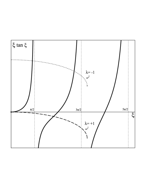
Figure 1: Graphical solution of $\xi\tan\xi=|\eta|-\lambda|\mathcal{\upsilon}|$ for the case $|\mathcal{\upsilon}|=5$. The solid lines stand for $\xi\tan\xi$, the dotted line for $|\eta|+|\mathcal{\upsilon}|$ and the dashed line for $|\eta|-|\mathcal{\upsilon}|$. The root $\xi=0$ is valid only for $\mathcal{\upsilon}>0$.

References

• [1] G. Petiau, Acad. R. Belg., A. Sci. Mém. Collect. 16, 2 (1936).
• [2] N. Kemmer, Proc. R. Soc. A 166, 127 (1938).
• [3] R. J. Duffin, Phys. Rev. 54, 1114 (1938).
• [4] N. Kemmer, Proc. R. Soc. A 173, 91 (1939).
• [5] M. Riedel, Relativistische Gleichungen fuer Spin-1-Teilchen, Diplomarbeit, Institute for Theoretical Physics, Johann Wolfgang Goethe-University, Frankfurt/Main (1979).
• [6] M. Nowakowski, Phys. Lett. A 244, 329 (1998).
• [7] J. T. Lunardi, B. M. Pimentel, R. G. Teixeira, and J. S. Valverde, Phys. Lett. A 268, 165 (2000).
• [8] R. F. Guertin and T. L. Wilson, Phys. Rev. D 15, 1518 (1977).
• [9] B. Vijayalakshmi, M. Seetharaman, and P. M. Mathews, J. Phys. A 12, 665 (1979).
• [10] T. R. Cardoso, L. B. Castro, and A. S. de Castro, J. Phys. A 43, 055306 (2010).
• [11] B. C. Clark, S. Hama, G. Kälbermann, R. L. Mercer, and L. Ray, Phys. Rev. Lett. 55, 592 (1985).
• [12] G. Kälbermann, Phys. Rev. C 34, 2240 (1986).
• [13] R. E. Kozack, B. C. Clark, S. Hama, V. K. Mishra, R. L. Mercer, and L. Ray, Phys. Rev. C 37, 2898 (1988).
• [14] R. E. Kozack, B. C. Clark, S. Hama, V. K. Mishra, G. Kälbermann, R. L. Mercer, and L. Ray, Phys. Rev. C 40, 2181 (1989).
• [15] L. J. Kurth, B. C. Clark, E. D. Cooper, S. Hama, R. L. Mercer, L. Ray, and G. W. Hoffmann, Phys. Rev. C 50, 2624 (1994).
• [16] R. C. Barret and Y. Nedjadi, Nucl. Phys. A 585, 311c (1995).
• [17] L. J. Kurth, B. C. Clark, E. D. Cooper, S. Hama, R. L. Mercer, L. Ray, and G. W. Hoffmann, Nucl. Phys. A 585, 335c (1995).
• [18] B. C. Clark, R. J. Furnstahl, L. K. Kerr, J. Rusnak, and S. Hama, Phys. Lett. B 427, 231 (1998).
• [19] Y. Nedjadi, S. Ait-Tahar, and R. C. Barret, J. Phys. A 31, 3867 (1998).
• [20] D. A. Kulikov, R. S. Tutik, and A. P. Yaroshenko, Mod. Phys. Lett. A 20, 43 (2005).
• [21] T. R. Cardoso, L. B. Castro, and A. S. de Castro, Can. J. Phys. 87, 857 (2009).
• [22] T. R. Cardoso, L. B. Castro, and A. S. de Castro, Can. J. Phys. 87, 1185 (2009).
• [23] T. R. Cardoso, L. B. Castro, and A. S. de Castro, Nucl. Phys. B (Proc. Suppl.) 199, 203 (2010).
• [24] L. B. Castro, T. R. Cardoso, and A. S. de Castro, Nucl. Phys. B (Proc. Suppl.) 199, 207 (2010).
• [25] A. S. de Castro, J. Math. Phys. 51, 102302 (2010).
• [26] L. B. Castro and A. S. de Castro, Phys. Lett. A 375, 2596 (2011).
• [27] A. S. de Castro, J. Phys. A 44, 035201 (2011).
• [28] Y. Nedjadi and R. C. Barret, J. Phys. G 19, 87 (1993).
Refer to caption