Detecting Chiral Edge States in the Hofstadter Optical Lattice

Abstract

We propose a realistic scheme to detect topological edge states in an optical lattice subjected to a synthetic magnetic field, based on a generalization of Bragg spectroscopy sensitive to angular momentum. We demonstrate that using a well-designed laser probe, the Bragg spectra provide an unambiguous signature of the topological edge states that establishes their chiral nature. This signature is present for a variety of boundaries, from a hard wall to a smooth harmonic potential added on top of the optical lattice. Experimentally, the Bragg signal should be very weak. To make it detectable, we introduce a “shelving method”, based on Raman transitions, which transfers angular momentum and changes the internal atomic state simultaneously. This scheme allows to detect the weak signal from the selected edge states on a dark background, and drastically improves the detectivity. It also leads to the possibility to directly visualize the topological edge states, using in situ imaging, offering a unique and instructive view on topological insulating phases.

Introduction

Recently, synthetic magnetic fields Lin et al. (2009) and spin-orbit couplings Lin et al. (2011) have been realized for ultra cold atoms using suitably arranged lasers that couple different internal states Dalibard et al. (2011). This opens the path to the experimental investigation of topological phases, such as quantum Hall (QH) states, topological insulators and superconductors, in a clean and highly controllable environment Bloch et al. (2008); Cooper (2008). Topological phases currently attract the attention of the scientific community for their remarkable properties, such as dissipationless transport and quantized conductivities Hasan and Kane (2010); Qi and Zhang (2011). In this context, the recent experimental realization of a staggered magnetic field in a 2D optical lattice, exploiting laser-induced gauge potentials, constitutes an important step in the field Aidelsburger et al. (2011) (cf. also Jiménez-García et al. (2012); Struck et al. (2012)). In the near future, large uniform magnetic flux should be reachable using related proposals Jaksch and Zoller (2003); Gerbier and Dalibard (2010); Jiménez-García et al. (2012); Struck et al. (2012), allowing optical-lattice experiments to explore the Hofstadter model Hofstadter (1976). The latter is the simplest tight-binding lattice model exhibiting topological transport properties: well-separated energy bands are associated to non-trivial topological invariants, the Chern numbers, leading to a quantized Hall conductivity when the Fermi energy is located in the bulk gaps Thouless et al. (1982); Kohmoto (1989). These transport properties are directly related to the existence of chiral edge states: while bulk excitations remain inert, these gapless states carry current along the edge of the system. According to the bulk-edge correspondence Hatsugai1993 ; Qi2006 , the Chern numbers characterizing the bulk bands determine the number of edge excitations and their chirality, which protects the edge transport against small perturbations.

In view of the experimental progress Aidelsburger et al. (2011); Jiménez-García et al. (2012); Struck et al. (2012), an important issue is to identify observables that provide unambiguous signatures of topological phases in a cold-atom framework Umucalilar et al. (2008); Goldman et al. (2010); Stanescu et al. (2010); Liu et al. (2010); Alba et al. (2011); Zhao et al. (2011); Kraus et al. (2012); Price2012 ; Buchhold2012 ; Dellabetta2012 . This is a crucial topic from an experimental point of view: Measuring the Hall conductivity is more difficult than for solid-state systems due to the absence of particle reservoirs coupled to the system. Several proposals exist for measuring the bulk topological invariants, e.g. based on spin-resolved time-of-flight Alba et al. (2011) or density measurements Umucalilar et al. (2008); Zhao et al. (2011). On the other hand, a direct detection of the edge states, associated with a proof of their chiral nature Stanescu et al. (2010); Liu et al. (2010), would witness the non-trivial topological order associated to cold-atom QH insulators. In this Letter, we propose a realistic and efficient scheme to probe the chiral edge states of the Hofstadter optical lattice, which we believe could be extended to any ultracold-atom setup emulating 2D topological phases.

The model

We study a two-dimensional fermionic gas confined in a square optical lattice and subjected to a uniform synthetic magnetic field $\bm{B}=B\hat{1}_{z}$ Jaksch and Zoller (2003); Gerbier and Dalibard (2010). The Hamiltonian is taken to be

$$\hat{H}_{0}= -J\sum_{m,n}\hat{c}^{\dagger}_{m+1,n}\hat{c}_{m,n}+e^{i2\pi\Phi m}\hat{c}^{\dagger}_{m,n+1}\hat{c}_{m,n}+\text{h.c.}$$

$$+\sum_{m,n}V_{\text{conf}}(r)\,\hat{c}^{\dagger}_{m,n}\hat{c}_{m,n},$$ (1)

with $\hat{c}_{m,n}$ the field operator defined at lattice site $(x=ma,y=na)$, $m,n\in\mathbb{Z}$, $J$ the tunneling amplitude, and $V_{\text{conf}}(r)$ a cylindrically symmetric confining potential. Eq. (1) describes non-interacting fermions on a lattice in the tight-binding regime, subjected to a vector potential $\bm{A}=(0,Bx,0)$ corresponding to $\Phi$ magnetic flux quanta per unit cell Hofstadter (1976).

It is instructive to first discuss the spectrum $E(k_{y})$ obtained by solving the Hamiltonian (1) on an abstract cylindrical geometry, without the potential $V_{\text{conf}}(r)$ ($k_{y}$ denotes the momentum along the closed direction $y$). For $\Phi=p/q$, where $p,q\in\mathbb{Z}$, the spectrum can be partitioned in terms of bulk states and topological edge states, as shown in Fig. 1(a). Bulk states exist in the absence of boundary and form $q$ well-separated subbands Hofstadter (1976). Because of its finite boundaries along $x$, this system also features topological edge states, which propagate along the edges of the cylinder Hatsugai1993 . They are located within the bulk energy gaps, with a quasi-linear local dispersion relation, $E/\hbar\approx v_{e}k_{y}$, where $v_{e}$ is the group velocity. In the spectrum represented in Fig. 1 (a), the two bulk gaps are associated to the quantized Hall conductivities $\sigma_{H}=\pm 1$ (in units of the conductivity quantum), as they host a single edge-state branch per edge, with opposite chirality $\text{sign}(v_{e})$. In the following, we set $\Phi=1/3$ and choose a Fermi energy $E_{F}=-1.5~{}J$ located within the first bulk gap, so that the fermionic gas forms a QH insulator with central density $n=1/3a^{2}$.

The clear partition of the single-particle spectrum into bulk states and topological edge states still holds in the experimental planar geometry and in the presence of the confining potential $V_{\text{conf}}(r)$, taken here of the form $V_{\text{conf}}(r)=J\left(r/r_{\rm edge}\right)^{\gamma}$. We illustrate the bulk-edge partition in Fig. 1 (b), which shows the discrete energy spectrum $\epsilon_{\alpha}$ for an infinite circular wall ($\gamma\rightarrow\infty$), with $r_{\text{edge}}=13a$: Similarly to the cylindrical case, we obtain bulk states within the energy bands and edge states (illustrated in Fig. 1(c)) within the bulk gaps. We stress that the number of edge excitation branches (relative to the number of physical edges) and their chirality do not depend on the particular geometry, as they are dictated by topological invariants associated to the bulk (see Hatsugai1993 ; Qi2006 and Supplementary Material). We verified that the above picture remains valid for finite confinements $\gamma\geq 2$: In agreement with their topological nature, edge states survive for a sufficiently weak confining potential that does not radically perturb the band structure.

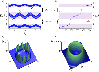
Figure 1: (Color online) (a) Single-particle energy spectrum $E=E(k_{y})$ for the cylindrical lattice subjected to a uniform flux $\Phi\!=\!1/3$, where $k_{y}$ is the momentum along the closed direction. The bulk states are found in the purple bands and the Hall conductivity $\sigma_{\text{H}}\!=\!\pm 1$ is indicated for $E_{\text{F}}\!\approx\!\pm 1.5J$. (b) Discrete energy spectrum for a circular infinite wall with $r_{\text{edge}}\!=\!13a$. The Fermi energy $E_{\text{F}}\!=\!-1.5J$ is represented by a red dotted line and $\alpha$ labels the single-particle states, i.e. $\hat{h}_{0}|\psi_{\alpha}\rangle\!=\!\epsilon_{\alpha}|\psi_{\alpha}\rangle$, where $\hat{h}_{0}$ is the single-particle Hamiltonian. (c) The amplitude $|\psi_{e}(m,n)|^{2}$ corresponding to the edge state at $\epsilon_{e}\approx-1.5J\!=\!E_{\text{F}}$ in (b). ​(d) The probe shape $f_{L}(m,n)\!=\!f_{L}(r)$ used to detect the edge state in (c).

Angular Momentum Spectroscopy :

Our aim is to design an experimental probe yielding a clear signature from the topological states. We note that a finite confining potential $V_{\text{conf}}(r)$ generally leads to non-topological edge states Stanescu et al. (2010); Hooley and Quintanilla (2004); Ott et al. (2004). However, QH edge states have a crucial property, their chirality (i.e. the sign of their angular velocity), that allows to distinguish them from the bulk and non-topological states by using a probe sensitive to angular momentum. Bragg spectroscopy, a form of momentum-sensitive light scattering, can provide such a probe Liu et al. (2010); Stanescu et al. (2010), as we now explain. In its usual implementation Stenger et al. (1999); Steinhauer et al. (2002), Bragg spectroscopy probes the linear momentum distribution. Here, we propose (a) to use a spatial mode carrying angular momentum in order to probe the angular momentum distribution, and (b) to shape the probing lasers to maximize the probability to excite an edge state. We consider two lasers denoted $1,2$ in high-order Laguerre-Gauss modes with optical angular momenta $l_{1,2}$, corresponding to the electric fields $E_{1,2}(r)=\sqrt{I_{1,2}}f_{l_{1},l_{2}}(r)\exp(-il_{1,2}\theta-i\omega_{1,2}t)$, where the radial mode functions are $f_{l}(r)\propto(r/r_{0})^{|l|}e^{-r^{2}/2r_{0}^{2}}$, and $(r,\theta)$ are polar coordinates. We assume that the beams are set off-resonance from a neighboring atomic transition, so that spontaneous emission can be neglected. This leads to a scattering Hamiltonian

$$\hat{H}_{\text{Bragg}}(t) =\hbar\Omega\sum_{\alpha\beta}\bigl{(}I_{\alpha\beta}^{q}e^{-i\omega_{L}t}+I_{\alpha\beta}^{-q}e^{i\omega_{L}t}\bigr{)}\hat{c}_{\alpha}^{\dagger}\hat{c}_{\beta},$$ (2)

$$I_{\alpha\beta}^{q} =\frac{1}{2}\int\text{d}\bm{x}\,\psi^{*}_{\alpha}(\bm{x})\psi_{\beta}(\bm{x})f_{L}(r)e^{iq\theta}.$$ (3)

Here, the index $q\!=\!l_{2}-l_{1}$ represents the amount of angular momentum transferred by the probe (in units of $\hbar$), $\hbar\omega_{L}\!=\!\hbar(\omega_{1}-\omega_{2})$ is the energy transfer, $\Omega$ is the Rabi frequency characterizing the strength of the atom-light coupling, and the probe profile is $f_{L}(r)\!=\!(r/r_{0})^{L}e^{-r^{2}/r_{0}^{2}}/\mathcal{N}_{L}$, with $L\!=\!|l_{1}|+|l_{2}|$ (cf. Fig. 1 (d)). The operator $\hat{c}_{\alpha}^{\dagger}$ creates a particle in the eigenstate $|\psi_{\alpha}\rangle$ of the unperturbed single-particle Hamiltonian, i.e. $\hat{h}_{0}|\psi_{\alpha}\rangle\!=\!\epsilon_{\alpha}|\psi_{\alpha}\rangle$.

Solving the time-dependent problem $\hat{H}_{0}+\hat{H}_{\text{Bragg}}(t)$ to first order, we write the many-body wave function as $|\Psi(t)\rangle\approx b_{0}(t)|0\rangle+\sum_{(k,l)}b_{kl}(t)e^{-i\omega_{kl}t}|kl\rangle$, where $|0\rangle=\prod_{\nu\leq E_{\text{F}}}\hat{c}_{\nu}^{\dagger}|\emptyset\rangle$ denotes the groundstate , and where $|kl\rangle=\hat{c}_{k}^{\dagger}\hat{c}_{l}|0\rangle$ denotes an excited state with a single fermionic excitation ($k>E_{\text{F}},l\leq E_{\text{F}}$) with energy $\hbar\omega_{kl}=(\epsilon_{k}-\epsilon_{l})>0$. With the initial conditions $(b_{0}(0)\!=\!1,b_{kl}(0)\!=\!0)$, the number of scattered particles (hereafter referred to as excitation fraction) is given by

$$N(q,\omega_{L})=\sum_{k,l}|b_{kl}(t)|^{2}=\Gamma_{\rm sc}t,$$ (4)

where the scattering rate $\Gamma_{\rm sc}$ is given by the Fermi golden rule (cf. Supplementary Material for details)

$$\Gamma_{\rm sc}=2\pi\Omega^{2}\sum_{k>E_{\text{F}},l\leq E_{\text{F}}}|I_{kl}^{q}|^{2}\delta^{(t)}(\omega_{kl}-\omega_{L}),$$ (5)

with $\pi t\delta^{(t)}(\omega)\!=\!(\sin(\omega t)/\omega)^{2}$. When the Fermi energy $E_{\text{F}}$ is set within a bulk gap, and for small intensities $\hbar\Omega\ll J$, the excitation fraction $N(q,\omega_{L})$ probes the dispersion relation $\epsilon_{e}=\epsilon_{\text{e}}(M)$ associated to the gapless edge states $|\psi_{e}\rangle$ that lie within this gap, where $M$ is a quantum number analogous to angular momentum (see Fig. 2 (a)). For an optimized probe shape (obtained for $r_{0}\approx r_{\text{edge}}/\sqrt{|L|/2}$), this can be deduced from the behavior of the overlap integrals $I_{kl}^{q}$ defined in Eq. 3. They are represented in the $\omega_{kl}-q$ plane in Fig. 2(b) for $\gamma=\infty$. At low frequencies $\omega_{kl}\ll J/\hbar$, we find a continuous alignment of resonance peaks $\omega_{kl}^{\text{res}}\approx\dot{\theta}_{\text{e}}q$. This reflects the linear dispersion relation $\epsilon/\hbar\approx\dot{\theta}_{\text{e}}M$ in the vicinity of the Fermi energy, and provides the angular velocity $\dot{\theta}_{\text{e}}\approx-0.07J/\hbar$ and the chirality (i.e. $\text{sign}(\dot{\theta}_{\text{e}})$) characterizing the edge states in the lowest bulk gap. We find that this result is in perfect agreement with a direct evaluation of the angular velocity . We emphasize that the edge states velocity highly depends on the boundary produced by the confinement: $\dot{\theta}_{\text{e}}$ significantly decreases as the potential $V_{\text{conf}}(r)$ is smoothened (e.g. $\dot{\theta}_{\text{e}}\approx-0.02J/\hbar$ for $\gamma=10$, $\dot{\theta}_{\text{e}}\approx-0.01J/\hbar$ for $\gamma=2$). The absence of substantial response for $q>0$ in Fig. 2 (b) clearly proves that our setup is effectively sensitive to the edge state chirality. Naturally, the signal obtained by setting the Fermi energy in the second bulk gap, or by reversing the sign of the magnetic flux $\Phi\rightarrow-\Phi$, would probe the opposite chirality.

We obtain the excitation fraction $N(q,\omega_{L})$ at finite times through a direct numerical resolution of the Schrödinger equation . A typical result is presented in Fig. 3(a), for $q=\pm 4$, emphasizing the three distinct regimes of light scattering: “edge-edge”, “bulk-edge” and “bulk-bulk”. The “edge-edge” regime corresponds to transitions solely performed between the edge states close to $E_{\text{F}}$: A sharp resonance peak is visible at $\omega_{L}^{\text{res}}\approx\dot{\theta}_{\text{e}}q\approx 0.3J/\hbar$ for $q=-4$, and stems from four transitions between edge states, as sketched in Fig. 2(a). Then, at higher frequencies, $\omega_{L}\approx J/\hbar$, small peaks witness allowed transitions between the lowest bulk band and the edge states located above $E_{\text{F}}$. Finally, for $\omega_{L}\approx 2J/\hbar$, many transitions between the two neighboring bulk bands lead to a wide and flat signal. This bulk-bulk response is significant for both $q=\pm 4$, as a consequence of the large density of excited states in this frequency range. We stress that a well focused probe allows to significantly reduce any signal of the bulk. In the following, we consider the quantity $N(q,\omega_{L})-N(-q,\omega_{L})$, which is zero for a system with time-reversal symmetry (cf. Fig. 3(b)). We have repeated the calculations for several potential shapes, finding no qualitative change (cf. Fig. 3(c)). Although it is advantageous to use a steep confining potential, the signal from the edge states is robust, even in a harmonic trap ($\gamma=2$).

The dispersion relation being almost linear close to $E_{\text{F}}$, the number of allowed transitions $|\psi_{l}\rangle\rightarrow|\psi_{k}\rangle$ scales with the probe parameter $q$ in the “edge-edge” regime (cf. Fig. 2(a)). Thus, one observes an increase of the peaks for increasing values of $|q|$ (cf. Fig.  3(d)). We stress that this progression only occurs in the “edge-edge” regime, namely when $q$ is chosen such that $\hbar\omega_{L}^{\text{res}}\approx\hbar\dot{\theta}_{\text{e}}q$ is smaller than the energy difference between $E_{\text{F}}$ and the closest bulk band. In the case illustrated in Fig.  3(d), the “edge-edge” regime is delimited by $|q_{\text{e-e}}|\lesssim 7$. Beyond $|q_{\text{e-e}}|$, the resonance peak enters the “bulk-edge” regime: The excitation fraction $N(q,\omega_{L})$ broadens, $N(-q,\omega_{L})$ is no longer negligible, and the linear dispersion relation is no longer probed. We thus conclude that a moderate value (here $|q|\sim 4$) is preferable to keep a narrow peak, well separated from the broader “edge-bulk” signal.

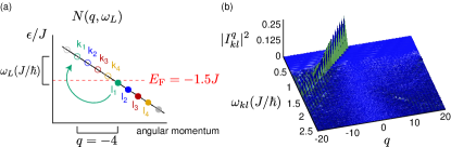
Figure 2: (Color online) (a) Sketch of the single-particle energy spectrum $\epsilon_{\alpha}$ and the transitions $|\psi_{l}\rangle\rightarrow|\psi_{k}\rangle$ probed by $N(q,\omega_{L})$, for $\omega_{L}\approx\omega_{kl}\ll J/\hbar$. (b) The amplitude $|I_{kl}^{q}|^{2}$, as a function of the probe parameter $q$ and excitation frequency $\omega_{kl}$, for $\Phi=1/3$, $E_{\text{F}}=-1.5J$, $L=13$ and $r_{0}=5.1a$. The confining potential is infinite ($\gamma=\infty$) and $r_{\text{edge}}=13a$.

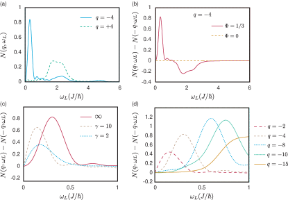
Figure 3: (a) Excitation fraction $N(q,\omega_{L})$ versus probe frequency, for an angular momentum transfer $q\!=\!\pm 4$. (b) $N(q,\omega_{L})\!-\!N(-q,\omega_{L})$ for $\Phi\!=\!0$ and $\Phi\!=\!1/3$. (c) $N(q,\omega_{L})\!-\!N(-q,\omega_{L})$ for several shapes of the trapping potential $V_{\text{conf}}(r)\!=\!J\left(r/r_{\rm edge}\right)^{\gamma}$ and $q\!=\!-4$. (d) Increasing then broadening of $N(q,\omega_{L})\!-\!N(-q,\omega_{L})$, for increasing $|q|$. In all the figures $\Omega\!=\!0.05J/\hbar$, $t\!=\!20\hbar/J$, $L\!=\!13$, $r_{0}\!=\!5.1a$, $r_{\text{edge}}\!=\!13a$, $\Phi\!=\!1/3$, $E_{\text{F}}\!=\!-1.5J$ and $\gamma=\infty$ (except in (c)).

Imaging the edge states

With respect to experimental detection, the Bragg scheme described above presents a major drawback. The associated signatures in the spatial or momentum densities are small perturbations on top of the strong “background” of unperturbed atoms. For a circular system with Fermi radius $R_{F}$, one can expect about $N_{\rm edge}\sim\Delta/\hbar\dot{\theta}_{e}\approx R_{F}\Delta/\hbar|v_{e}|$ edge states, with $\Delta$ the bulk energy gap and $v_{e}$ the group velocity (cf. above). Using the parameters from Fig. 3(a), one finds $N_{\rm edge}\sim 20$ while the total number of atoms in the calculation is $N\sim 200$. Scaling to more realistic numbers for an experiment ($N\sim 10^{4}$), and noting that the number of scattered atoms is at most a fraction of $N_{\rm edge}$, we conclude that one should be able to detect a few tens of atoms at best on top of the signal coming from $\sim 10^{4}$ unperturbed ones: This is a significant experimental challenge with present-day technology. One possibility to avoid this difficulty is to use an alternate detection scheme, where the probe also changes the atomic internal state. The probe signal can then be measured against a dark background (without unperturbed atoms), which allows powerful imaging methods to be used (e.g. large aperture microscopy, as recently demonstrated for quantum gases in optical lattices Bakr et al. (2009); Sherson et al. (2009)) .

We present in Fig. 4(a) a possible implementation suitable for two-electron atoms with ultra-narrow optical transitions, inspired by the electron shelving method. In the following, we use the particular case of ¹⁷¹Yb atoms for illustration (see also Supplementary Material). The ground $g$ and excited $e$ states have nuclear spin $I=1/2$, leading to ground $\{g_{\downarrow},g_{\uparrow}\}$ and excited $\{e_{\downarrow},e_{\uparrow}\}$ manifolds. The Zeeman degeneracies are split by a real and relatively strong magnetic field $B\sim 100~{}$G. The states $g_{\uparrow}$ and $e_{\uparrow}$ are initially populated, as laser coupling between these two states is used to generate the artificial gauge field leading to Eq. (1) (cf. methods described in Jaksch and Zoller (2003); Gerbier and Dalibard (2010)). In order to probe the $(+)=\{g_{\uparrow},e_{\uparrow}\}$ system, one introduces a weaker additional laser, coupling $g_{\uparrow}\rightarrow e_{\downarrow}$. A crucial point is to ensure that topological edge states have the same structure in the initial and final states. To this end, the initially unpopulated states $(-)=\{g_{\downarrow},e_{\downarrow}\}$ are also coupled by a laser generating the same gauge field as for $(+)$. After the probe pulse, atoms in the $g$ manifold are dispatched (possibly detected) using an auxiliary imaging transition $g\rightarrow f$. Crucially, atoms in the $e$ manifold are not in resonance with the imaging light and are therefore unaffected. The $e_{\downarrow}$ atoms are subsequently brought down to the $g$ manifold using, e.g., adiabatic-passage techniques, and they are finally detected, without stray contributions from unperturbed atoms in other internal states.

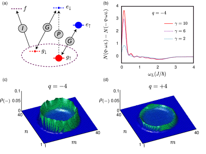
Figure 4: (a) Detection scheme for a two-electron atom, where $g$ is the electronic ground state, $e$ a metastable excited state and $f$ a second excited state with short radiative lifetime, suitable for imaging. The coupling lasers $G$ induce an artificial gauge field and the probe laser $P$ allows to detect edge states (cf. text). The circles indicate relative populations in each state after the probe pulse. (b) Excitation fraction versus probe frequency, for several potential shapes. (c)-(d) Density $\rho_{(-)}(m,n)$ for $q=\pm 4$, $\gamma=10$ and $\omega_{L}=0.14J/\hbar$. The probe and system parameters in (b)-(d) are the same as in Fig.3.

To analyze the effect of this probe, we consider a simplified level scheme with two internal states only, denoted by the indices $(\pm)$. We suppose that only the $(+)$ sector is initially populated. The spatial profile of the coupling laser is similar to the one used for Bragg excitations, but now the Pauli principle does not restrict the available final states, since the state $(-)$ is initially unoccupied. The calculation proceeds as before, with initial $|0\rangle=\prod_{\epsilon_{\nu}\leq E_{F}}\hat{c}_{\nu,+}^{\dagger}|\emptyset\rangle$ and final $|kl\rangle=\hat{c}_{k,-}^{\dagger}\hat{c}_{l,+}|0\rangle$ states. We write the coupling to the probe as

$$\hat{H}_{\text{Shelving}}(t)=\hbar\Omega\sum_{\alpha\beta}I_{\alpha\beta}^{q}\hat{c}_{\alpha,-}^{\dagger}\hat{c}_{\beta,+}e^{-i\omega_{L}t}+\text{h.c.},$$ (6)

where the operator $\hat{c}_{\alpha,(\pm)}^{\dagger}$ creates a particle of the $(\pm)$ sector in the eigenstate $|\psi_{\alpha}\rangle$, and where $I_{\alpha\beta}^{q}$ has the same definition as in Eq. (3), since $\hat{h}_{+}=\hat{h}_{-}=\hat{h}_{0}$. We also suppose that $\hbar\Omega\ll J$ to neglect higher order excitations.

The excitation fraction $N(q,\omega_{L})-N(-q,\omega_{L})$ is represented in Fig. 4(b), showing a clear resonance peak at low frequencies $\hbar\omega_{L}\ll J$. Interestingly, this result shows that the low-energy regime is still governed by the chiral edge states located in the bulk gap, although transitions are now allowed for all the states below $E_{\text{F}}$, including the bulk states (see Supplementary Material). Indeed, the signal $N(q,\omega_{L})-N(-q,\omega_{L})$ remains small and flat in the “edge-bulk” region, while the chiral “edge-edge” peak stands even clearer than in the Bragg case (since more “edge-edge” transitions are allowed between states of same chirality). By setting the probe parameters $(q,\omega_{L})$ close to a resonance peak, one can now populate edge states into the $(-)$ sector and directly visualize them using state-selective imaging. The corresponding density $\rho_{(-)}(m,n)=\langle\Psi(t)|\hat{n}_{(-)}(m,n)|\Psi(t)\rangle$ is illustrated in Figs. 4(c)-(d) for $q=\pm 4$. The clear difference between the two images, obtained with different signs of $q$ but otherwise identical setups, is a direct proof of the chiral nature of the edge excitations populated by the probe. Thus, we have demonstrated that our state-dependent probe (6), combined with in situ imaging, provides an efficient method to identify topological edge states in a cold-atom experiment. We believe that this method could be generalized to any cold-atom setup subjected to synthetic gauge potentials that emulate 2D topological phases, even in the presence of interactions or disorder.

We thank the F.R.S-F.N.R.S, DARPA (Optical lattice emulator project), the Emergences program (Ville de Paris and UPMC) and ERC (Manybo Starting Grant) for financial support. We are grateful to J. Dalibard, S. Nascimbène, F. Chévy, C. Morais Smith, P. Öhberg, W. Hofstetter, M. Buchhold and D. Cocks for inspiring discussions and comments.

Appendix A The bulk-edge correspondence and the circular geometry

In this work, we consider the Hofstadter optical lattice described by the Hamiltonian in Eq. (1). In an optical-lattice experiment, the atoms are confined by a cylindrically symmetric confining potential, which we take of the form

$$V_{\text{conf}}(r)=J\left(r/r_{\rm edge}\right)^{\gamma},$$ (7)

where the parameters $J$, $r_{\rm edge}$ and $\gamma$ are defined in the main text. We are interested in the detection of chiral edge states, which propagate along the circular edge of this system. In the solid-state framework, these chiral states are responsible for the quantum Hall effect Hasan and Kane (2010); Qi and Zhang (2011); Hatsugai1993 . In this appendix, we recall how these topological edge states are indeed related to the concept of topological invariants, which guarantee their robustness against small external perturbations.

The fundamental concept which relates the chiral edge states illustrated in Fig. 1 (c) to topological invariants is the so-called bulk-edge correspondence Hatsugai1993 ; Qi2006 . This theorem stipulates that when specific topological invariants associated to the bulk bands are non-zero, the presence of edge states at the boundaries is guaranteed and that their chirality (i.e. their orientation of propagation along the edge) is fixed. Moreover, the edge states energies are located within the bulk gaps, as illustrated in Fig. 1 (a). Here, the topological invariants are defined on the first Brillouin zone, or equivalently on an abstract two-dimensional torus $\mathbb{T}^{2}$, as a result of periodic boundary conditions applied to both spatial directions (more precisely, the topological invariants are defined on a principle fibre bundle $P(\text{U(1)},\mathbb{T}^{2})$, which is based on the two-torus $\mathbb{T}^{2}$). These topological indices are the Chern numbers $N_{\nu}$, which are associated to each bulk band $E_{\nu}(\bm{k})$ through the Thouless-Kohmoto-Nightingale-Nijs expression (TKNN) Thouless et al. (1982)

$$N_{\nu}=\frac{i}{2\pi}\int_{\mathbb{T}^{2}}\langle\partial_{k_{x}}u_{\nu}(\bm{k})|\partial_{k_{y}}u_{\nu}(\bm{k})\rangle-(k_{x}\leftrightarrow k_{y})\textnormal{d}\bm{k},$$ (8)

where $|u_{\nu}(\bm{k})\rangle$ is the single-particle eigenstate of the Hamiltonian with energy $E_{\nu}(\bm{k})$, and $\bm{k}=(k_{x},k_{y})\in\mathbb{T}^{2}$ is the quasi-momentum. When the Fermi energy $E_{\text{F}}$ is exactly located in a bulk gap, the Hall conductivity is directly related to the Chern numbers,

$$\sigma_{H}=\sum_{E_{\nu}<E_{\text{F}}}N_{\nu},$$ (9)

which can be directly derived from the Kubo formalism Thouless et al. (1982); Kohmoto (1989). Here the conductivity is expressed in units of the conductivity quantum.

For the specific case studied in this work, where we set the magnetic flux $\Phi=1/3$, the bulk energy spectrum splits into three energy bands, which have the associated Chern numbers $N_{1}=-1$, $N_{2}=2$ and $N_{3}=-1$. Therefore, when the Fermi energy lies in the first [resp. second] bulk gap, the Hall conductivity corresponds to $\sigma_{H}=-1$ [resp. $\sigma_{H}=+1$], as illustrated in Fig. 1 (a)-(b). These results, which are derived from the toroidal geometry, are summarized in Table 2.

The bulk-edge correspondence dictates the following result: if we solve the same model (1) on an open geometry (i.e. a system with boundaries), gapless edge states will appear in the bulk gaps. Moreover the number of edge-state branches is given by the modulus of the Hall conductivity in (9), and their chirality by $\text{sign}(\sigma_{H})$. This can be easily visualized by solving the model (1) on an abstract cylinder (with $V_{\text{conf}}=0$). The corresponding energy spectrum $E(k_{y})$ is illustrated in Fig. 1 (a) and is described in the main text. Since the cylinder has two physical edges, we note that the first bulk gap in Fig. 1 (a) hosts two edge-state branches with opposite orientations (i.e. one for each physical edge) Hatsugai1993 . The presence of a single edge excitation (per physical edge) is in agreement with the fact that $|\sigma_{H}|=|N_{1}|=1$ when the Fermi energy is located in this bulk gap: this is precisely the bulk-edge correspondence, which is summarized in Table 2.

We stress that the number of edge-state branches (per physical edge) is independent of the boundary geometry, as it is given by a sum of topological indices (9) associated to the bulk bands. Therefore, when considering the realistic circular geometry produced by the confining potential $V_{\text{conf}}(r)$ in Eq. (7), one obtains the same edge-state structure propagating along the circular edge $r=r_{\text{edge}}$ as the one obtained from the abstract cylinder discussed above: the number of edge-state branches and the chirality deduced from them are identical, as these properties do not depend on the chosen geometry. However, let us comment on the fact that the boundaries do affect the dispersion relations, and thus the angular velocity, of the edge states (cf. main text). Here, the bulk-edge correspondence indicates that the lowest bulk gap in Fig. 1(b), which corresponds to the circular geometry, hosts a single edge-state branch associated to a negative angular velocity, since the corresponding Hall conductivity $\sigma_{H}=-1$ is solely governed by the topological expression (9). Furthermore, the edge-state branch present in the second bulk gap corresponds to the opposite chirality, since $\sigma_{H}=+1$ when the Fermi energy is in the highest gap. These results have been verified by directly computing the angular velocity of the edge states,

$$\dot{\theta}_{\text{e}} =(i/\hbar)\sum_{m,n}\psi_{e}^{*}(m,n)[\hat{h}_{0},\hat{\theta}]\psi_{e}(m,n),$$

$$\!\!\!\!\!\!\!\!=\frac{Ji}{\hbar}\sum_{m,n}\bigl{(}\theta(m+1,n)-\theta(m,n)\bigr{)}\psi^{*}_{e}(m,n)\psi_{e}(m+1,n)$$

$$\!\!\!\!\!\!\!\!+\bigl{(}\theta(m-1,n)-\theta(m,n)\bigr{)}\psi^{*}_{e}(m,n)\psi_{e}(m-1,n)$$

$$\!\!\!\!\!\!\!\!+e^{i2\pi\Phi m}\bigl{(}\theta(m,n+1)-\theta(m,n)\bigr{)}\psi^{*}_{e}(m,n)\psi_{e}(m,n+1)$$

$$\!\!\!\!\!\!\!\!+e^{-i2\pi\Phi m}\bigl{(}\theta(m,n-1)-\theta(m,n)\bigr{)}\psi^{*}_{e}(m,n)\psi_{e}(m,n-1),$$

where $\theta(m,n)=\text{atan2}\bigl{(}(n-N/2),(m-N/2)\bigr{)}$ and $m,n=1,\dots,N$, and also indirectly through the Bragg signals, as illustrated in this Appendix (cf. Fig. 5).

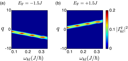
Figure 5: (Color online) The amplitude $|I_{kl}^{q}|^{2}$, as a function of the probe parameter $q$ and excitation frequency $\omega_{kl}$, for $\Phi=1/3$, $L=13$ and $r_{0}=5.1a$. The confining potential is infinite ($\gamma=\infty$) and $r_{\text{edge}}=13a$. (a) $E_{\text{F}}=-1.5J$ and (b) $E_{\text{F}}=+1.5J$. The angular velocity of the edge states present in the first [resp. second] bulk gap is $\dot{\theta}_{\text{e}}\approx\omega_{kl}^{\text{res}}/q\approx-0.07J/\hbar$ [resp. $\dot{\theta}_{\text{e}}\approx+0.07J/\hbar$]. Thus, the two bulk gaps are associated with opposite chiralities, in agreement with the bulk-edge correspondence in Table 2.

Appendix B Angular Momentum Spectroscopy

The interaction between the Bragg lasers and the atoms is described by the Hamiltonian

$$\hat{H}_{\text{Bragg}}(t)=\hbar\Omega\bigl{(}\hat{W}_{q}e^{-i\omega_{L}t}+\hat{W}_{-q}e^{i\omega_{L}t}\bigr{)},$$ (10)

$$\hat{W}_{q}=\sum_{\alpha\beta}I_{\alpha\beta}^{q}\hat{c}_{\alpha}^{\dagger}\hat{c}_{\beta},$$ (11)

$$I_{\alpha\beta}^{q}=\frac{1}{2}\int\text{d}\bm{x}\,\psi^{*}_{\alpha}(\bm{x})\psi_{\beta}(\bm{x})f_{L}(r)e^{iq\theta}.$$ (12)

Here, the operator $\hat{c}_{\alpha}^{\dagger}$ creates a particle in the eigenstate $|\psi_{\alpha}\rangle$ of the unperturbed single-particle Hamiltonian, i.e. $\hat{h}_{0}|\psi_{\alpha}\rangle=\epsilon_{\alpha}|\psi_{\alpha}\rangle$ (cf. main text). Solving the time-dependent problem $\hat{H}_{0}+\hat{H}_{\text{Bragg}}(t)$ to first order, we write the many-body wave function as

$$|\psi(t)\rangle =b_{0}(t)|0\rangle+\sum_{\mu}b_{\mu}(t)e^{-iE_{\mu}t/\hbar}|\Psi_{\mu}\rangle,$$

$$\approx b_{0}(t)|0\rangle+\sum_{(k,l)}b_{kl}(t)e^{-i\omega_{kl}t}|kl\rangle,$$ (13)

where $|0\rangle=\prod_{\nu\leq E_{\text{F}}}\hat{c}_{\nu}^{\dagger}|\emptyset\rangle$ denotes the groundstate at zero temperature, and

$$|kl\rangle=|1\dots 1\underbrace{0}_{l}1\dots 1\underbrace{|}_{E_{\text{F}}}0\dots 0\underbrace{1}_{k}0\dots 0\rangle,$$ (14)

where $k>E_{\text{F}},l\leq E_{\text{F}}$ and $\omega_{kl}=(\epsilon_{k}-\epsilon_{l})/\hbar>0$. Here we have restricted the full Hilbert space to the subspace spanned by the ground state and the excited states that are coupled to it to first order in the perturbation (10).

Setting the initial condition $(b_{0}(0)=1,b_{kl}(0)=0)$, one finds

$$b_{kl}(t)=-i\Omega\biggl{(}I_{kl}^{q}S_{kl}^{-}(\omega_{L})e^{i\Delta_{kl}^{-}t}+(I_{lk}^{q})^{*}S_{kl}^{+}(\omega_{L})e^{i\Delta_{kl}^{+}t}\biggr{)},$$ (15)

where $S_{kl}^{\pm}(\omega_{L})=\sin(\Delta_{kl}^{\pm}t)/\Delta_{kl}^{\pm}$, $\Delta_{kl}^{\pm}=(\omega_{kl}\pm\omega_{L})/2$. The number of scattered atoms, or excitation fraction, is then given by

$$N(q,\omega_{L})=\sum_{k,l}|b_{kl}(t)|^{2},$$

$$=\Omega^{2}\sum_{k,l}|I_{kl}^{q}S_{kl}^{-}(\omega_{L})e^{i\Delta_{kl}^{-}t}+(I_{lk}^{q})^{*}S_{kl}^{+}(\omega_{L})e^{i\Delta_{kl}^{+}t}|^{2}.$$ (16)

In the long-time limit, and neglecting the anti-resonnant term $(\propto e^{i\Delta_{kl}^{+}t})$, this yields the standard Fermi golden rule

$$N(q,\omega_{L})=2\pi\Omega^{2}t\sum_{k>E_{\text{F}},l\leq E_{\text{F}}}|I_{kl}^{q}|^{2}\delta^{(t)}(\omega_{kl}-\omega_{L}),$$ (17)

where $\delta^{(t)}(\omega)\!=(1/\pi t)(\sin(\omega t)/\omega)^{2}\overset{t\rightarrow\infty}{\xrightarrow{\hskip 28.45274pt}}\delta(\omega)$. The expression (17) emphasizes the explicit relation between the excitation fraction $N(q,\omega_{L})$ and the rates $|I_{kl}^{q}|^{2}$ presented in Fig. 2 (b).

At finite times, it is preferable to evaluate the excitation fraction through a numerical evaluation of the Schrödinger equation

$$i\hbar\frac{\text{d}b_{kl}(t)}{\textnormal{d}t}=\hbar\Omega\sum_{n,m}W_{kl;nm}(t)b_{nm}(t)e^{i(E_{kl}-E_{nm})t/\hbar},$$ (18)

where $W_{kl;nm}(t)\!=\!\langle kl|\hat{W}(t)|nm\rangle$ and $\hat{W}(t)=\hat{W}_{q}e^{-i\omega_{L}t}+\hat{W}_{-q}e^{i\omega_{L}t}$. The many-body wavefunction is still restricted to the first-order subspace but off-resonant terms and deviations from the long-time limit are included. For the reasonable finite times and small Rabi frequencies $\Omega\ll J/\hbar$ used in our calculations (cf. Figs. (3)-(4)), we find that the excitation fraction obtained from a numerical evaluation of Eq. (18) is in perfect agreement with Eq. (16). Note that we use excitation times of several $\hbar/J$, typically, which seem experimentally realistic. This is long enough to resolve the edge-edge resonance but still too short to neglect the broadening due to the finite pulse time (cf. Figs. (3)-(4)(b)).

Appendix C The Shelving Method

The scattering Hamiltonian considered in the “shelving method” has the form

$$\hat{H}_{\text{Shelving}}(t)=\hbar\Omega\bigl{(}\hat{W}_{q}^{\text{sh}}e^{-i\omega_{L}t}+\bigl{(}\hat{W}_{q}^{\text{sh}}\bigr{)}^{\dagger}e^{i\omega_{L}t}\bigr{)},$$ (19)

$$\hat{W}_{q}^{\text{sh}}=\sum_{\alpha\beta}I_{\alpha\beta}^{q}\hat{c}_{\alpha(-)}^{\dagger}\hat{c}_{\beta(+)},$$ (20)

where the operator $\hat{c}_{\alpha(\pm)}^{\dagger}$ creates a particle of the $(\pm)$ sector in the eigenstate $|\psi_{\alpha}\rangle$, and where $I_{\alpha\beta}^{q}$ has the same definition as in Eq. (12), since $\hat{h}_{(-)}=\hat{h}_{(+)}=\hat{h}_{0}$.

In this scheme, we suppose that only the $(+)$ sector is initially populated, such that the initial and excited states have the following forms

$$|0\rangle\!=\!|1\dots 1\underbrace{|}_{E_{\text{F}}}0\dots 0\rangle_{(+)}|0\dots 0\rangle_{(-)},$$ (21)

$$|kl\rangle\!=\!|1\dots 1\underbrace{0}_{l}1\dots 1\underbrace{|}_{E_{\text{F}}}0\dots 0\rangle_{{}_{(+)}}|0\dots 0\underbrace{1}_{k}0\dots 0\rangle_{{}_{(-)}},$$ (22)

where we suppose that $\Omega\ll J/\hbar$ to neglect higher order excitations. We note that $k$ is no longer restricted by the Pauli principle, such that $\omega_{kl}=(\epsilon_{k}-\epsilon_{l})/\hbar$ may now take negative values. We follow the same treatment as for the Bragg scheme and we obtain the excitation fraction as

$$N(q,\omega_{L})=2\pi\Omega^{2}t\sum_{l\leq E_{\text{F}}}\sum_{k}|I_{kl}^{q}|^{2}\delta^{(t)}(\omega_{kl}-\omega_{L}),$$ (23)

which differs from Eq. (17) by the fact that the final states $k$ are now unrestricted. However, we stress that the sum over the initial states, $\sum_{l\leq E_{\text{F}}}$ in Eq. (23), is still restricted by the Pauli principle: for $\omega_{L}\!\ll\!J/\hbar$ and when $E_{\text{F}}\!=\!-1.5J$, this allows to probe the edge states that are located in the first bulk gap only. This important fact leads to the asymmetry highlighted in Figs. 4(c)-(d), which demonstrates the specific chirality of these edge states (cf. main text).

We finally stress that the condition

$$\hat{h}_{(-)}\!=\!\hat{h}_{(+)}\!=\!\hat{h}_{0},$$

is necessary in order to probe the edge-state structure. Indeed, if we consider a simpler scheme in which the $(-)$ sector is no longer subjected to a synthetic gauge potential, we find that $N(q,\omega_{L})-N(-q,\omega_{L})\approx 0$. This observation shows that our scheme requires that the edge states of the $(-)$ sector should have the same chirality than the initially populated edge-states of the $(+)$ sector, i.e. both systems should be subjected to the same magnetic flux (cf. Appendix D).

Appendix D Detection scheme using state-changing transitions: example for ¹⁷¹Yb atoms

We give here a more detailed account of the detection scheme using ¹⁷¹Yb atoms (see Fig. 4 (a)). The ground $g$ and metastable excited $e$ states have zero electronic angular momentum but nuclear spin $I=1/2$. We denote the Zeeman manifolds $\{g_{\downarrow},g_{\uparrow}\}$ and $\{e_{\downarrow},e_{\uparrow}\}$ in the ground ${}^{1}S_{0}$ and ${}^{3}P_{0}$ excited states, respectively. The states $g_{\uparrow}$ and $e_{\uparrow}$ are initially populated, as laser coupling between these two states is used to generate the artificial gauge field Jaksch and Zoller (2003); Gerbier and Dalibard (2010) leading to Eq. (1). A crucial point is to ensure that topological edge states have the same structure in the initial and final states (cf. Appendix C). To this end, the initially unpopulated states $(-)=\{g_{\downarrow},e_{\downarrow}\}$ are also coupled by a laser generating the same gauge field as for $(+)$. The degeneracies are split by a relatively strong magnetic field, $\Delta E_{a_{i}}=-g_{a}m_{i}B$, where $a=e,g$ denotes the ground or excited manifold, $i=\uparrow/\downarrow$, $m_{i}=\pm 1/2$ the nuclear spin quantum number, $g_{g}/h\approx-750~{}$Hz/G, and $g_{e}/h\approx-1250$ Hz/G. A bias field $B\sim 100~{}$G thus leads to Zeeman shifts $\sim\pm 25~{}$kHz on the $\pi$ transitions and $\sim\pm 100~{}$kHz on the $\sigma^{\pm}$ transitions: these shifts are very large compared to the Rabi frequencies of both the gauge-field and probe lasers, which can thus be treated independently.

In order to probe the $(+)=\{g_{\uparrow},e_{\uparrow}\}$ system, one introduces a weaker additional laser, coupling $g_{\uparrow}\rightarrow e_{\downarrow}$. Due to the gauge coupling, a population will build up in the $g_{\downarrow}$ state as well (roughly equal to that in the $e_{\downarrow}$ state since $\Omega\ll J$). Those atoms will be missing in the final detection step. After probing, the lattice sites are isolated by rapidly raising the lattice height and switching off the artificial gauge field. Atoms in the $g$ manifold are dispatched (possibly detected) using an auxiliary imaging transition $g\rightarrow f$. A natural choice for ¹⁷¹Yb is $f\!=$${}^{1}\!P_{1}$, with a line width $\gamma_{f}/2\pi\approx 28~{}$MHz much larger than any Zeeman splitting in $g$ or $e$ (thus prohibiting independent detection of atoms depending on their spin $\downarrow/\uparrow$). Crucially, atoms in the $e$ manifold are not in resonance with the imaging light and are therefore unaffected. The $e_{\downarrow}$ atoms are subsequently brought down to the $g$ manifold using, e.g., adiabatic passage techniques, leaving the $e_{\uparrow}$ state unaffected. A further imaging pulse allows to detect those atoms, initially excited by the probe pulse. One might worry that a fraction of atoms from the $e_{\uparrow}$ state could end up being transferred too, thus contaminating the final edge signal. Fortunately, the off-resonant excitation rate to “wrong” states will be smaller than the resonant rate by a factor scaling as $\sim(\Omega/\Delta_{Z})^{2}$, with $\Delta_{Z}\sim|g_{e}-g_{g}|B/2$ a typical Zeeman splitting. Taking for example the parameters given in Gerbier and Dalibard (2010), one has $J/h\approx 100~{}$Hz, and $\Omega\sim 0.05J/\hbar\sim 2\pi\times 20~{}$Hz, making the final contamination of $g_{\downarrow}$ by $e_{\uparrow}$ negligible ($\sim 10^{-5}$).

Chern numbers associated to the two lowest bulk bands:	$N_{1}=-1$	$N_{2}=2$
Hall conductivity in the two bulk gaps (from Kubo formula):	$\sigma_{H}(E_{\text{F}}\in 1\text{st gap})=-1$	$\sigma_{H}(E_{\text{F}}\in 2\text{nd gap})=+1$
Chirality of the edge states inside the bulk gaps (circular geometry):	$\text{sign}(\sigma_{H}(1\text{st gap}))$=(-)	$\text{sign}(\sigma_{H}(2\text{nd gap}))$=(+)

Table 1: The Hofstadter model with $\Phi=1/3$: Chern numbers, Hall conductivity and edge-state configurations.

Two-dimensional Geometries:	torus (abstract)	cylinder (abstract)	circular (realistic)
Number of 1D boundaries:	0	2	1
Chern number of the bulk band $E_{\nu}(\bm{k})$:	$N_{\nu}$	–	–
Hall conductivity for $E_{\text{F}}\in r$th bulk gap (from Kubo formula):	$\sigma_{H}^{(r)}=\sum_{\nu=1}^{r}N_{\nu}$	–	–
Number of edge-state branches in the $r$th bulk gap:	–	$2\,|\sigma_{H}^{(r)}|$	$|\sigma_{H}^{(r)}|$
Chirality of the edge states located in the $r$th bulk gap:	–	$\text{sign}(\sigma_{H}^{(r)})$	$\text{sign}(\sigma_{H}^{(r)})$

Table 2: The bulk-edge correspondence: Topological Chern numbers (defined in the bulk) and the properties of gapless edge excitations for the three geometries described in the text. Note that for the cylinder, the edge states at the two different physical edges have opposite velocities Hatsugai1993 ; Qi2006 .

References

- Lin et al. (2009) Y.-J. Lin, R. L. Compton, K. Jiménez-García, J. V. Porto, and I. B. Spielman, Nature 462, 628 (2009).
- Lin et al. (2011) Y.-J. Lin, K. Jiménez-García, and I. B. Spielman, Nature 471, 83 (2011).
- Dalibard et al. (2011) J. Dalibard, F. Gerbier, G. Juzeliūnas, and P. Öhberg, Rev. Mod. Phys. 83, 1523 (2011).
- Bloch et al. (2008) I. Bloch, J. Dalibard, and W. Zwerger, Rev. Mod. Phys 80, 885 (2008).
- Cooper (2008) N. R. Cooper, Advances in Physics 57, 539 (2008).
- Hasan and Kane (2010) M. Z. Hasan and C. L. Kane, Rev. Mod. Phys. 82, 3045 (2010).
- Qi and Zhang (2011) X.-L. Qi and S.-C. Zhang, Rev. Mod. Phys. 83, 1057 (2011).
- Aidelsburger et al. (2011) M. Aidelsburger, M. Atala, S. Nascimbène, S. Trotzky, Y.-A. Chen, and I. Bloch, Phys. Rev. Lett. 107, 255301 (2011).
- Jiménez-García et al. (2012) K. Jiménez-García, L. J. LeBlanc, R. A. Williams, M. C. Beeler, A. R. Perry, and I. B. Spielman, arXiv cond-mat.quant-gas (2012), eprint 1201.6630v1.
- Struck et al. (2012) J. Struck, C. Ölschläger, M. Weinberg, P. Hauke, J. Simonet, A. Eckardt, M. Lewenstein, K. Sengstock, and P. Windpassinger, arXiv cond-mat.quant-gas (2012), eprint 1203.0049v1.
- Jaksch and Zoller (2003) D. Jaksch and P. Zoller, New Journal of Physics 5, 56 (2003).
- Gerbier and Dalibard (2010) F. Gerbier and J. Dalibard, New Journal of Physics 12, 033007 (2010).
- Hofstadter (1976) D. R. Hofstadter, Phys. Rev. B 14, 2239 (1976).
- Thouless et al. (1982) D. J. Thouless, M. Kohmoto, M. P. Nightingale, and M. den Nijs, Phys. Rev. Lett. 49, 405 (1982).
- Kohmoto (1989) M. Kohmoto, Phys. Rev. B 39, 11943 (1989).
- (16) Y. Hatsugai, Phys. Rev. Lett. 71, 3697 (1993); Y. Hatsugai, Phys. Rev. B 48, 11851 (1993).
- (17) X.-L. Qi, Y.-S. Wu and S.-C. Zhang, Phys. Rev. B 74, 045125 (2006).
- Umucalilar et al. (2008) R. O. Umucalilar, H. Zhai, and M. O. Oktel, Phys. Rev. Lett. 100, 070402 (2008).
- Goldman et al. (2010) N. Goldman, I. Satija, P. Nikolic, A. Bermudez, M. Martin-Delgado, M. Lewenstein, and I. Spielman, Physical Review Letters 105, 255302 (2010).
- Stanescu et al. (2010) T. D. Stanescu, V. Galitski, and S. Das Sarma, Phys. Rev. A 82, 013608 (2010).
- Liu et al. (2010) X.-J. Liu, X. Liu, C. Wu, and J. Sinova, Phys. Rev. A 81, 033622 (2010).
- Alba et al. (2011) E. Alba, X. Fernandez-Gonzalvo, J. Mur-Petit, J. K. Pachos, and J. J. Garcia-Ripoll, Phys. Rev. Lett. 107, 235301 (2011).
- Zhao et al. (2011) E. Zhao, N. Bray-Ali, C. Williams, I. Spielman, and I. Satija, Physical Review A 84, 063629 (2011).
- Kraus et al. (2012) C. V. Kraus, S. Diehl, P. Zoller, and M. A. Baranov, arXiv cond-mat.quant-gas (2012), eprint 1201.3253v1.
- (25) H. M. Price and N. R. Cooper, Phys. Rev. A 85, 033620 (2012).
- (26) M. Buchhold, D. Cocks, and W. Hofstetter, arXiv:1204.0016v1.
- (27) B. Dellabetta, T. L. Hughes, M. J. Gilbert and B. L. Lev, arXiv:1202.0060v1.
- Ott et al. (2004) H. Ott, E. de Mirandes, F. Ferlaino, G. Roati, V. Türck, G. Modugno, and M. Inguscio, Phys. Rev. Lett. 93, 120407 (2004).
- Hooley and Quintanilla (2004) C. Hooley and J. Quintanilla, Phys. Rev. Lett. 93, 080404 (2004).
- Stenger et al. (1999) J. Stenger, S. Inouye, A. P. Chikkatur, D. M. Stamper-Kurn, D. E. Pritchard, and W. Ketterle, Phys. Rev. Lett. 82, 4569 (1999).
- Steinhauer et al. (2002) J. Steinhauer, R. Ozeri, N. Katz, and N. Davidson, Phys. Rev. Lett. 88, 120407 (2002).
- Bakr et al. (2009) W. S. Bakr, J. I. Gillen, A. Peng, S. Fölling, and M. Greiner, Nature 462, 74 (2009).
- Sherson et al. (2009) J. F. Sherson, C. Weitenberg, M. Endres, M. Cheneau, I. Bloch, and S. Kuhr, Nature 467, 68 (2009).