The Laplacian on planar graphs and graphs on surfaces

1 Introduction

By a resistor network, or simply network, we mean here a graph $\mathcal{G}=(V,E)$ with vertices $V$ and (undirected) edges $E$, and $c$ a positive real-valued function on the edges. The value $c_{e}$ is the conductance of the edge $e$.

The Laplacian on a network $(\mathcal{G},c)$ is the linear operator $\Delta\colon\mathbb{R}^{V}\to\mathbb{R}^{V}$ defined by

$$(\Delta f)(v)=\sum_{v^{\prime}\sim v}c_{vv^{\prime}}(f(v)-f(v^{\prime})).$$ (1)

Here the sum is over neighbors $v^{\prime}$ of $v$.

The Laplacian is the most basic operator on a network, and has countless uses in all areas of mathematics. We study here some specific properties of the Laplacian on networks embedded on surfaces, and in particular on the simplest surfaces: the plane, the annulus, the torus.

Our goals will be to focus on a few topological, probabilistic and combinatorial applications. Specifically, our three main interconnected goals are to discuss:

1. The discrete EIT (Electrical Impedance Tomography) problem: reconstructing the network from boundary measurements. For planar networks, the classification due to Yves Colin de Verdière of Dirichlet-to-Neumann operators [6, 7],

2. The connections with the random spanning tree model developed by Curtis, Ingerman and Morrow [8] and Wilson and myself [19, 20], and

3. The characteristic polynomial of $\Delta$ on an annulus and torus based on joint work with Okounkov and Sheffield [16], Okounkov [15], and in [14].

Acknowledgements. Large parts of section 4 were developed by Colin de Verdière [6] and Curtis, Ingerman and Morrow [8]. I thanks them for explanations and discussions.

The rest of this paper includes material developed in various projects jointly with Alexander Goncharov, Andrei Okounkov, Scott Sheffield, and David Wilson. In particular some of the material is lifted directly out of work in progress with David Wilson [21], whom I thank for allowing it to be included here.

The main new results in the current paper are Lemma 4.11 and Theorems 5.1, 6.1, and 7.1.

2 Background

2.1 Electrical Impedance Tomography

The classical Calderón problem is to determine the electrical conductivity of a region in $\mathbb{R}^{2}$ or $\mathbb{R}^{3}$ by making boundary measurements of the type: fix the voltage along the boundary and measure the resulting current flow out of the region.

This problem has concrete applications in medical imaging, nondestructive materials testing, etc. In these settings it is called Electrical Impedance Tomography (EIT). It is widely used because it is easy and cheap to implement: basically it is very easy to apply a low voltage to pretty much any conductive material and measure the resulting current flow.

In this paper we study the discrete version of EIT. Given a resistor network (a finite graph in which every edge is a resistor), understand its internal structure from boundary measurements. There is a very nice solution for planar networks. For networks on more general surfaces we are beginning to have a better understanding but much more remains to be done.

For a network $\mathcal{G}$ on a surface with nontrivial topology there is closely related question, even when there is no boundary, which is to understand the determinant of the “bundle Laplacian” as a function on the moduli space of flat connections on bundles on $\mathcal{G}$.

We shall see how these questions are related below.

2.2 Spanning trees

One of the combinatorial tools involved in the study of discrete EIT is the model of (random) spanning trees, and related objects called cycle-rooted spanning forests on networks. Kirchhoff [22] was the first to see the connection between spanning trees and the Laplacian on a network: he showed that the Laplacian determinant in fact counts spanning trees.

The random spanning tree measure (or UST, for Uniform Spanning Tree) has for the past $20$ years been a remarkably successful and rich area of study in probability theory. The random spanning tree as a probability model goes back to at least work of Temperley [31], who gave a bijection between spanning trees on the square grid and domino tilings. Aldous and Broder [1, 2] in the 1980s showed a connection between spanning trees and random walk, giving an algorithm for sampling a UST based on the simple random walk on the network. Pemantle [28] showed that the unique path between two points in a UST has the same distribution as the loop-erased random walk (LERW) between those two points. Wilson [32] extended this to give a quick and elegant method of sampling a uniform spanning tree in any graph. Burton and Pemantle [4] proved that the edges of the uniform spanning tree form a “determinantal process”, that is there is a matrix $T$ indexed by the edges such that the probability that some set of edges $\{e_{1},\dots,e_{k}\}$ is in the UST is $\det(T(e_{i},e_{j})_{1\leq i,j\leq k})$. The matrix $T$ is built from the Green’s function of $\Delta$.

The UST on the grid $\mathbb{Z}^{2}$ received particular attention due to the conformal invariance properties of its scaling limit (limit when the mesh size of the grid goes to zero). In particular in [13] we showed that the “winding field” of the UST on $\mathbb{Z}^{2}$ (which measure the winding of the branches around faces) converges in the scaling limit to the Gaussian free field, a conformally invariant random function on $\mathbb{R}^{2}$. In [25] Lawler, Schramm and Werner showed the convergence of the branches of the UST on $\mathbb{Z}^{2}$ in the scaling limit to the conformally invariant process $\text{SLE}_{2}$.

As mentioned above, Temperley [31] gave a bijection between spanning trees and the dimer model on the square grid; this was later generalized to arbitrary graphs in [17] and [18], pointing to a very close relation between the UST and the dimer model. Many of the results discussed below are inspired by the corresponding results in the dimer model.

2.3 Characteristic polynomials

To a network on an annulus we can associate a polynomial $P(z)$ which is the determinant of the line-bundle Laplacian $\Delta$ for a flat line bundle with monodromy $z\in\mathbb{C}^{*}$ around a generator of the homology of the annulus. One can think of this as the determinant of the Laplacian acting on the space of $z$-quasiperiodic functions: “locally defined” functions whose values are multiplied by $z$ under analytic continuation counterclockwise around the annulus.

The polynomial $P$ is real and symmetric (that is, $P(z)=P(1/z)$). There is a nice characterization of those $P$ which occur: they are those with positive constant coefficient, and whose roots are real, positive and distinct except for a double root at $z=1$. See Theorem 6.1 below.

For a network on the torus one can associate a two-variable polynomial $P(z_{1},z_{2})$ in a similar way: it is the determinant of the Laplacian for a flat line bundle with monodromy $z_{1},z_{2}$ around generators of $\pi_{1}$ of the torus. This polynomial plays an important role in understanding the structure and large-scale properties of the random spanning tree model on a periodic planar graph [4, 16]. Like in the case of the annulus there is a characterization of those $P(z_{1},z_{2})$ which occur: the curve $\{P(z_{1},z_{2})=0\}$ is a Harnack curve which is symmetric $(P(z_{1},z_{2})=P(z_{1}^{-1},z_{2}^{-1})$), satisfies $P(1,1)=0$ and has positive constant coefficient. See the definition of Harnack curve in section 7.4. One can show that in fact any Harnack curve satisfying the above properties arises from the characteristic polynomial of some toral network.

A more recent development in networks on the torus is the understanding of the integrable dynamical system underlying them. Here the dynamical system is not related to the flow of current in the network, but is a dynamical system on the space of conductances assigned to the edges in the network. It is the restriction of an integrable Hamiltonian dynamical system on a larger space (the space of line bundles on bipartite networks on the torus) to a Lagrangian subvariety. See [12]. We will not discuss this here, mostly because we don’t yet have a very good understanding of this system except as an invariant subvariety of a larger system.

For networks on other surfaces $\Sigma$ one can also define a characteristic polynomial $P=\det\Delta$ which is a regular function on the representation variety of $\pi_{1}(\Sigma)$ into $\text{SL}_{2}(\mathbb{C})$. Here much less is known about the structure of $P$. See however Theorem 8.1 below.

Finally, one would like to consider a network on a general surface with boundary, and understand properties of the boundary measurement map (for the appropriate bundle Laplacian) and to what extent it determines the network. We are still far from this goal but the cases of simple topology or small boundary hint that there is an interesting answer.

3 Networks

By a network we mean a connected finite graph $\mathcal{G}=(V,E)$ with a positive real-valued function $c$ on the edges called the conductance function, and a usually nonempty set of vertices $\mathcal{N}$ called nodes or terminals or boundary vertices. These are the simplest type of electrical networks, with resistors only.

The nodes are indexed from $1$ to $n$. Let $I$ be the set of non-node vertices; elements of $I$ are referred to as internal vertices.

3.1 Laplacian

The Laplacian on a network $\mathcal{G}$ is the operator $\Delta:\mathbb{R}^{V}\to\mathbb{R}^{V}$ defined for $f\in\mathbb{R}^{V}$ by (1). Since $\mathbb{R}^{V}$ has a natural basis, consisting of functions $\delta_{v}$ which are $1$ at $v$ and zero elsewhere, we often write $\Delta$ as a matrix $\Delta=(\Delta_{vv^{\prime}})_{v,v^{\prime}\in V}$ where $\Delta_{vv^{\prime}}=-c_{vv^{\prime}}$ if $v,v^{\prime}$ are adjacent and the diagonal entries are $\Delta_{vv}=\sum_{v^{\prime}\sim v}c_{vv^{\prime}}.$ See for example (8) which is the Laplacian of the graph of Figure 1.

Associated to the Laplacian is the quadratic form $Q$ on $\mathbb{R}^{V}$ defined as

$$Q(f)=\langle f,\Delta f\rangle=\sum_{v\sim v^{\prime}}c_{vv^{\prime}}(f(v)-f(v^{\prime}))^{2}$$ (2)

which is called the Dirchlet energy of $f$. Here $\langle,\!\rangle$ is the natural inner product in which the basis $\{\delta_{v}\}_{v\in V}$ is orthonormal.

From the expression (2) we see that $\Delta$ is positive semidefinite with kernel consisting of the constant functions (we assume unless stated otherwise that $\mathcal{G}$ is connected).

Another useful operator is the incidence matrix $d$, defined as follows. Fix an (arbitrary) orientation for each edge $e$, so that $e_{+}$ and $e_{-}$ are its head and tail. Define $d\colon\mathbb{R}^{V}\to\mathbb{R}^{E}$ by the formula

$$df(e)=f(e_{+})-f(e_{-}).$$

Then it is easy to verify that

$$\Delta=d^{*}{\cal C}d,$$

where ${\cal C}$ is the diagonal matrix of conductances, and $d^{*}$ is the transpose of $d$ (its adjoint for the inner product $\langle,\rangle$ above): for an element $w\in\mathbb{R}^{E}$ we have

$$d^{*}w(v)=\sum_{e\to v}w(e)$$

where the sum is over the edges $e$ containing endpoint $v$, and directed towards $v$. We can call $df$ the gradient of the function $f$ and $d^{*}w$ the divergence of the flow $w$.

Note that we can write the Dirichlet energy as

$$Q(f)=\langle df,{\cal C}df\rangle$$

where here $\langle,\!\rangle$ is the natural inner product on $\mathbb{R}^{E}$.

3.2 The Laplacian with boundary

If $B\subset V$ is a subset of vertices and $I=V\setminus B$, we can define an operator $\Delta_{B}:\mathbb{R}^{I}\to\mathbb{R}^{I}$ called the Dirichlet Laplacian with boundary $B$ by the same formula

$$\Delta_{B}f(v)=\sum_{v^{\prime}\sim v}c_{vv^{\prime}}(f(v)-f(v^{\prime})),$$

where here $v\in I$ and the sum is over all neighbors of $v$ in $V$ (not just those in $I$).

As a matrix $\Delta_{B}$ is just a submatrix of the full Laplacian $\Delta$: the submatrix indexed by $I$.

3.3 The Dirichlet problem

A function $f\in\mathbb{R}^{V}$ is said to be harmonic at $v$ if $\Delta f(v)=0$. By (1) this simply means that $f(v)$ is a weighted average of the values of $f$ at the neighboring vertices, where the weights are proportional to the conductances.

A function is harmonic if it is harmonic at all vertices. On a finite connected graph a harmonic function must be constant, since the kernel of $\Delta$ consists of constant functions only.

Suppose $B$ is a nonempty set boundary vertices and $u$ is a function on $B$. A function $f$ on $V$ which is harmonic on $I=V\setminus B$ and agrees with $u$ on $B$ is said to be harmonic with Dirichlet boundary conditions on $B$. Such functions satisfy a maximum principle: their maximum (and minimum) values occur on $B$ (because of the above observation about weighted averages).

Given this fact it is not hard to see that, if $B$ is nonempty, then $\Delta_{B}$ is invertible: any function $f$ in the kernel of $\Delta_{B}$ can be extended to a function on $V$ taking values zero on $B$; it is thus a harmonic function with Dirichlet boundary conditions at $B$. By the maximum principle it must take its maximum and minimum on $B$, where it has value $0$. Thus $f$ must be identically zero.

The Dirichlet problem is the problem of finding, for a given function $u$ on $B$, a function $f$ on $V$ which is equal to $u$ on $B$ and harmonic on $I=V\setminus B$: find $f$ satisfying

$$\Delta f(v)=0 \text{ for }v\in V\setminus B$$ (3)

$$f(v)=u(v) \text{ for }v\in B.$$

The function $f$ is called the harmonic extension of $u$. For finite networks the solution to the Dirichlet problem is straightforward using invertibility of $\Delta_{B}$. Alternatively, the solution $f$ is the function with boundary values $u$ and which minimizes the Dirichlet energy $Q(f)$. Convexity of $Q$ implies that there is a unique solution.

A function on $\mathcal{G}$ which is harmonic on $I$ is a solution to the Dirichlet problem with boundary $B$. Such a function is also called an equilibrium potential.

3.4 The Dirichlet problem and the response matrix

For a network we will take $\mathcal{N}$, the set of nodes, to play the role of the boundary vertices (which we called $B$ above). Given a function $u$ on $\mathcal{N}$, let $f_{u}$ be the harmonic extension of $u$. Then $\Delta f_{u}(v)$, restricted to $\mathcal{N}$, is a (generally nonzero) function of $v\in\mathcal{N}$. The map $\Lambda:u\mapsto\Delta f_{u}|_{\mathcal{N}}$ is a linear map $\Lambda:\mathbb{R}^{\mathcal{N}}\to\mathbb{R}^{\mathcal{N}}$ called the Dirichlet-to-Neumann map of the network. For certain conventional reasons we often prefer to work with $L=-\Lambda$ and refer to $L$ as the response matrix. See the next section for an example.

We can describe $\Lambda$ as a matrix as follows. Suppose we index the vertices so that vertices in $\mathcal{N}$ come first. Then we can write $\Delta$ in block form as

$$\Delta=\left(\begin{matrix}A&B\\ B^{t}&C\end{matrix}\right),$$

where $A$ has rows and columns indexed by the nodes $\mathcal{N}$ and $C$ has rows and columns indexed by the internal vertices; $C$ is just the matrix of the Dirichlet Laplacian $\Delta_{\mathcal{N}}$.

The Dirichlet problem (3) can be written as follows: find $f_{I}$ on the internal vertices $I$ so that

$$\left(\begin{matrix}A&B\\ B^{t}&C\end{matrix}\right)\left(\begin{matrix}u\\ f_{I}\end{matrix}\right)=\left(\begin{matrix}g\\ 0\end{matrix}\right),$$

for a function $g$ which is the desired function of $u$. We can split this into two linear equations

$$Au+Bf_{I} = g$$ (4)

$$B^{t}u+Cf_{I} = 0.$$ (5)

This second equation can be solved as

$$f_{I}=-C^{-1}B^{t}u.$$ (6)

(Here $C$ is invertible, as discussed above).

One can then plug in this value of $f_{I}$ in the first equation to get

$$Au-BC^{-1}B^{t}u=g,$$

that is, $\Lambda u=g$ where $\Lambda$ is the matrix $\Lambda=A-BC^{-1}B^{t}$. Thus

$$L=-A+BC^{-1}B^{t}.$$ (7)

We see from this expression that $L$ is symmetric, since $A$ and $C$ are symmetric. In fact $\Lambda$ is positive semidefinite (and $L$ is negative semidefinite), with kernel consisting solely of the constant functions. This follows from the fact that

$$\langle u,\Lambda u\rangle=\langle f,\Delta f\rangle\geq 0$$

where $f$ is the harmonic extension of $u$ (one can check this using (6)).

3.4.1 Example

Let $\mathcal{G}$ be the network of Figure 1 with three nodes $\{v_{1},v_{2},v_{3}\}$, one internal vertex $v_{4}$

Figure 1: The ‘Y’ network.

and three edges with conductances $c_{1},c_{2},c_{3}$. We have

$$\Delta=\begin{bmatrix}c_{1}&0&0&-c_{1}\\ 0&c_{2}&0&-c_{2}\\ 0&0&c_{3}&-c_{3}\\ -c_{1}&-c_{2}&-c_{3}&c_{1}+c_{2}+c_{3}\end{bmatrix}.$$ (8)

Using formula (7) we have

$$L = -\begin{pmatrix}c_{1}&0&0\\ 0&c_{2}&0\\ 0&0&c_{3}\end{pmatrix}+\begin{pmatrix}-c_{1}\\ -c_{2}\\ -c_{3}\end{pmatrix}(\frac{1}{c_{1}+c_{2}+c_{3}})\begin{pmatrix}-c_{1}&-c_{2}&-c_{3}\end{pmatrix}$$ (9)

$$= \begin{pmatrix}\frac{-c_{1}c_{2}-c_{1}c_{3}}{c_{1}+c_{2}+c_{3}}&\frac{c_{1}c_{2}}{c_{1}+c_{2}+c_{3}}&\frac{c_{1}c_{3}}{c_{1}+c_{2}+c_{3}}\\ \frac{c_{2}c_{1}}{c_{1}+c_{2}+c_{3}}&\frac{-c_{2}c_{1}-c_{2}c_{3}}{c_{1}+c_{2}+c_{3}}&\frac{c_{2}c_{3}}{c_{1}+c_{2}+c_{3}}\\ \frac{c_{3}c_{1}}{c_{1}+c_{2}+c_{3}}&\frac{c_{3}c_{2}}{c_{1}+c_{2}+c_{3}}&\frac{-c_{3}c_{1}-c_{3}c_{2}}{c_{1}+c_{2}+c_{3}}\end{pmatrix}.$$

3.5 Electrical interpretation

Associated to a function $f$ (called potential or voltage) on a network is a flow $\omega$ on the edges (called current) defined by

$$\omega(e)={\cal C}df(e)=c_{e}(f(e_{+})-f(e_{-})).$$

Here ${\cal C}$ is the diagonal matrix of edge conductances and $df(e)=f(e_{+})-f(e_{-})$ is the gradient of $f$.

Ohm’s law states that ${\cal C}df(e)$ is the flow across edge $e$ when the vertices are held at potentials $f(e_{+})$ and $f(e_{-})$, and the resistance on the edge is $1/c_{e}$, the reciprocal of the conductance.

Kirchhoff’s network equations state that when the boundary nodes are held at fixed potentials, the internal vertices will attain potentials $f$ in such a way that the flow of current induced by Ohm’s law in the network has the property that the current entering an internal vertex equals the current exiting that vertex. In other words the divergence $d^{*}\omega$ of the current $\omega$ is zero at internal vertices. Thus $d^{*}{\cal C}d(f)=0$ at every internal vertex, so $f$ is the harmonic extension of $u$.

This allows us to give $L_{ij}$ the following electrical interpretation: Hold all nodes except $i$ at potential $0$, and node $i$ at potential $1$. Then for the resulting current flow, $L_{ij}$ is the current exiting the network at node $i$. This current is positive: the potentials at internal vertices are in $[0,1]$ (in fact in $(0,1)$) by the maximum principle for harmonic functions, so the current at edges adjacent to $j$ is directed towards $j$. Similarly one shows $L_{ii}<0$.

4 Circular planar networks

By a circular planar network (CPN) we mean a connected finite graph $\mathcal{G}=(V,E)$ embedded in the plane, with a positive real-valued function $c$ on the edges called the conductance function, and a nonempty set of vertices $\mathcal{N}$ on the outer face called nodes or terminals. (There may be other vertices on the outer face as well). The reason it is a circular planar network is that the network can be drawn inside the disk with the nodes on the boundary circle.

The nodes are ordered in counterclockwise order from $1$ to $n$. Let $I$ be the set of non-node vertices; elements of $I$ are referred to as internal vertices. The non-exterior faces of $\mathcal{G}$ are referred to as interior faces; we consider $\mathcal{G}$ to also have $n$ exterior faces, with the $i$th exterior face comprising the region between nodes $i$ and $i+1$, and having boundary consisting of the edges along the “outer face” of $\mathcal{G}$ between node $i$ and $i+1$.

4.1 Conjugate harmonic function

If $\mathcal{G}$ is a circular planar network, a harmonic function $f$ on $\mathcal{G}$ with Dirichlet boundary conditions on $\mathcal{N}$ has a conjugate harmonic function $g$ defined (up to an additive constant) on the faces of $\mathcal{G}$ by the condition ${\cal C}df=\partial g$, where $\partial$ is the difference operator on the dual graph $\mathcal{G}^{\prime}$: if $e=vv^{\prime}$ is an edge of $\mathcal{G}$ and $F_{1},F_{2}$ are the adjacent faces, so that $F_{1}$ is left of $e$ when $e$ is traversed from $v$ to $v^{\prime}$, then

$$c_{e}(f(v^{\prime})-f(v))=g(F_{1})-g(F_{2}).$$ (10)

The harmonicity of $f$ implies that these equations are consistent around a vertex; by summing along paths one sees that the value of $g$ is defined consistently on all faces, once one choose a value of $g$ at any starting face. Thus these equations define $g$ uniquely up to a global additive constant. The function $g$ is harmonic for the operator $\partial^{*}{\cal C}^{-1}\partial$. That is, one puts conductances on the dual edges which are the inverses of the conductances on the primal edges.

The pair $(f,g)$ is sometimes written as $f+ig$ and is called a discrete analytic function since the equations (10) play the role of the discrete Cauchy-Riemann equation.

If $f$ is harmonic with Dirichlet boundary conditions then $g$ will be harmonic on $\mathcal{G}^{\prime}$ with Dirichlet boundary conditions, that is, $g$ is harmonic on interior vertices of $\mathcal{G}^{\prime}$ (that is, on non-exterior faces of $\mathcal{G}$).

4.2 Characterization of response matrices

The response matrix is a fundamental matrix associated to a network. A natural question is: what properties of the network are reflected in its response matrix?

The basic properties of $L$ shown in the previous section are that

1. $L$ is real and symmetric,

2. $L$ is negative semidefinite,

3. The kernel of $L$ consists of the constant functions, and

4. $L_{ij}>0$ if $i\neq j$, and $L_{ii}<0$.

(It is not hard to see that property 2 is implied by the others).

Any matrix satisfying the above properties is in fact the response matrix of some (not necessarily planar) network: it suffices to take a complete graph on $n$ vertices, declare that each vertex is a node, and put conductance $L_{ij}$ on the edge $ij$ connecting vertices $i$ and $j$.

The question is much more interesting in the case of circular planar networks. In this case there is a beautiful characterization of response matrices in terms of minors, due to Colin de Verdière [6].

Given two disjoint subsets $A,B$ of the nodes of a circular planar network, we say that $A$ and $B$ are noninterlaced if they are contained in disjoint intervals of nodes with respect to the circular order. That is, if $a<b<c<d$ are nodes then it is never the case that $a,c\in A$ and $b,d\in B$.

Theorem 4.1 ([6]).

$L$ is the response matrix of a connected circular planar network if and only if $L$ is symmetric, with kernel consisting of the constant functions, and for any disjoint noninterlaced subsets of nodes $A$ and $B$ with $|A|=|B|$, we have $\det L_{A}^{B}\geq 0$, where $L_{A}^{B}$ is the submatrix of $L$ whose rows index $A$ and columns index $B$.

There are two parts of this theorem, the necessity of the conditions and the existence of a network for any $L$ satisfying the conditions. Both have interesting proofs which we will discuss.

We define a network to be well-connected if all noninterlaced minors $\det L_{A}^{B}$ are strictly positive. In [6] Colin de Verdière shows that the space of well-connected circular planar networks on $n$ nodes is homeomorphic to an open ball of dimension $\begin{pmatrix}n\\ 2\end{pmatrix}$. More about this in section 4.4.2

4.3 Groves

As one can see from (7), the response matrix entries are rational functions of the conductances. Surprisingly, the off-diagonal entries are subtraction free rational functions of the conductances, that is, ratios of polynomials with positive coefficients; in fact the coefficients are all $1$ or $0$ (see for example (9)). This is a strong indication that these polynomials are counting some type of combinatorial objects.

Indeed, that is one of the ideas in the Curtis-Ingerman-Morrow proof (see [8]) of necessity in Theorem 4.1 above, which we discuss in this section.

4.3.1 Spanning trees

A spanning tree of a graph is a subset of edges which is a tree, that is, contains no cycles, and is spanning, that is, connects all vertices. Equivalently one can say that a spanning tree is a maximal set of edges (with respect to inclusion) that has no cycles.

For a network $\mathcal{G}$ with conductances $c$ on its edges, one can define the weight $w(T)$ of a spanning tree $T$ to be the product of the conductances of its edges, $w(T)=\prod_{e\in T}c_{e}$.

The most important theorem about spanning trees is that the Laplacian determinant is the weighted sum of spanning trees (this is also called the partition sum).

Theorem 4.2 (Matrix-Tree Theorem [22]).

Let $\det_{0}\Delta$ be the product of the nonzero eigenvalues (with multiplicity) of $\Delta$ for a connected network $\mathcal{G}$. Then

$$\frac{1}{|\mathcal{G}|}{\det}_{0}\Delta=\sum_{T}w(T).$$

Here the sum is over spanning trees of $\mathcal{G}$.

This theorem is usually attributed to Kirchhoff [22]. An equivalent formulation is that the partition sum $Z:=\sum_{T}w(T)$ is equal to the reduced determinant of $\Delta$, which is the determinant of $\Delta$ after removing any row and column; since $\Delta$ is symmetric and constant functions are in the kernel any choice of row and column gives the same reduced determinant.

Proof of Theorem 4.2, sketch. Several proofs of the Matrix-tree Theorem are known; the classical one we present uses the Cauchy-Binet Theorem which is a formula for computing the determinant of a product of two nonsquare matrices: it states that if $X$ is an $n\times m$ matrix and $Y$ is $m\times n$ with $m\geq n$ then

$$\det XY=\sum_{B}\det(X^{B})\det(Y_{B})$$ (11)

where $B$ runs over all choices of $n$ column indices for $X$, $X^{B}$ is the $n\times n$ minor of $X$ defined by columns $B$ and $Y_{B}$ is the $n\times n$ minor of $Y$ defined by rows $B$.

For the Matrix-Tree Theorem, let $\Delta_{\bar{1},\bar{1}}$ be the submatrix of $\Delta$ obtained by removing row $1$ and column $1$. Then $\Delta_{\bar{1},\bar{1}}=d^{*}_{\bar{1}}{\cal C}d_{\bar{1}}$ where $d_{\bar{1}}$ is obtained from $d$ by removing column $1$.

One now uses $X=d_{\bar{1}}^{*}$ and $Y={\cal C}d_{\bar{1}}$ in (11). Each $B$ in (11) is a set of $|V|-1$ edges; we claim that the nonzero summands in (11) are precisely the sets of edges which form spanning trees. If $B$ forms a tree, its edges can be directed towards the removed vertex. Then in the definition of $\det d_{\bar{1},B}$ as an expansion over the symmetric group,

$$\det d_{\bar{1},B}=\sum_{\sigma\in S_{n-1}}(-1)^{\sigma}d_{2\sigma(2)}\dots d_{n\sigma(n)},$$

the only nonzero term is the one whose permutation $\sigma$ matches each vertex to the edge adjacent to it and closer to the root. Thus $\det d_{\bar{1},B}=\pm 1$. If edges in $B$ do not form a tree, then there must be more than one component; the function on vertices which is $1$ on a component not containing the removed vertex and zero elsewhere is in the kernel of $d_{\bar{1},B}$, so $\det d_{\bar{1},B}=0$.

Finally, the determinant of the diagonal submatrix $\det{\cal C}_{B}^{B}$ for a tree $B$ is the product of the edge weights, and $\det d_{\bar{1},B}^{*}=\det d_{\bar{1},B}=\pm 1$. So

$$\det(d^{*}_{\bar{1},B}{\cal C_{B}^{B}}d_{\bar{1},B})=w(T).$$

This completes the proof. $\square$

The spanning tree measure is the probability measure on spanning trees of a graph in which the probability of a tree is proportional to its weight. In the special case that the conductances are all $1$ this is the uniform measure on spanning trees (UST measure); each tree has probability $\frac{1}{\kappa}$ where $\kappa$ is the determinant of the reduced Laplacian of the conductance-$1$ network; $\kappa$ is sometimes called the complexity of the network.

Cayley’s formula [5], first proved by Borchhardt [3] gives the number spanning trees of the complete graph $K_{n}$ to be $n^{n-2}$. This follows easily from the above theorem since

$$\Delta=\begin{pmatrix}n-1&-1&\dots&-1\\ -1&n-1&-1&\vdots\\ \vdots&&\ddots&-1\\ -1&\dots&-1&n-1\end{pmatrix}$$

whose eigenvalues are $n$ with multiplicity $n-1$ and $0$ with multiplicity $1$.

4.3.2 Groves from minors of $L$

On a network with nodes $\mathcal{N}$, a grove is a subset of the edges, each of whose components is a tree containing one or more nodes. In other words it is a “spanning forest” in which each component is connected to the boundary (and isolated vertices are considered components, so there are no isolated internal vertices). See Figure 2. We allow a component to contain more than one node; for example a spanning tree is a special case of a grove.

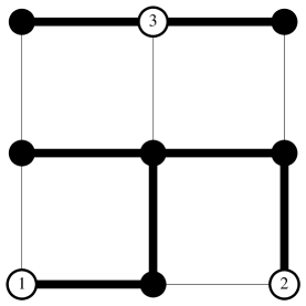
Figure 2: A grove of type $12|3$ (nodes are in white; internal vertices in black).

Groves can be put into equivalence classes depending on how their components partition the nodes. Given a partition $\pi$ of the nodes, let $S_{\pi}$ be the set of groves in which each component contains exactly all the nodes of a part of $\pi$. For example when there are three nodes the partitions are: $1|2|3$ where each node is in a separate component, $1|23$ where nodes $2$ and $3$ are in the same component different from $1$, and likewise $2|13,3|12,$ and finally $123$ where all nodes are in the same component. More generally groves in the set $S_{1|2|\dots|n}$, that is, in which each component contains exactly one node, are called uncrossings. The groves in $S_{12\dots n}$ are spanning trees.

Note that for circular planar graphs not all partitions $\pi$ are possible; for a partition to be obtained by a grove it must be planar. For example $13|24$ is not the partition of any grove on a circular planar graph.

The probability measure on spanning trees extends to a probability measure on groves: the weight of a grove is the product of its edge weights, and the probability of a grove is $\frac{1}{Z}$ times its weight, where $Z=\sum_{T}w(T)$ is the weighted sum of all groves.

For each partition $\pi$ we denote by $Z_{\pi}$ the weighted sum of groves of type $\pi$. Then $Z=\sum_{\pi}Z_{\pi}$, and the probability that a random grove has type $\pi$ is $\frac{Z_{\pi}}{Z}$. We define $Z_{\mathrm{unc}}=Z_{1|2|\dots|n}$ to be the partition sum for uncrossings, and $Z_{\text{tree}}=Z_{12\dots n}$ to be the weight sum of spanning trees.

All minors of the response matrix have combinatorial interpretations in terms of groves, for example when $i\neq j$ we prove in Theorem 4.3 below that

$$L_{ij}=\frac{Z_{\pi(ij|\text{rest different})}}{Z_{\mathrm{unc}}}=\frac{\mathrm{Pr}(\pi(ij|\text{rest different}))}{\mathrm{Pr}({\mathrm{unc}})}$$

where $\pi(ij|\text{rest different})$ is the partition in which all nodes are in separate components except for $i$ and $j$ which are in the same component. More generally, we have the following combinatorial interpretation of all minors of $L$ (a closely related result can be found in [8]):

Theorem 4.3 ([20]).

Let $Q,R,S,T\subset\mathcal{N}$ be a partition of $\mathcal{N}$ into four sets with $|R|=|S|$ (and some of which may be empty). Then $\det L_{R\cup T}^{S\cup T}$ is the ratio of two terms: the denominator is $Z_{\mathrm{unc}}$; the numerator is a signed weighted sum of groves of $\mathcal{G}_{T}$, the graph $\mathcal{G}$ in which all nodes in $T$ are considered internal vertices, the nodes in $Q$ are in singleton parts, and in which nodes in $R$ are paired with nodes in $S$, with the sign being the sign of the pairing permutation:

$$\det L_{R\cup T}^{S\cup T}=(-1)^{|T|}\sum_{\text{{permutations} $\rho$}}(-1)^{\rho}\frac{Z\big{[}{}_{r_{1}}^{s_{\rho(1)}}|\cdots|_{r_{k}}^{s_{\rho(k)}}|q_{1}|\cdots|q_{\ell}\big{]}}{Z_{\mathrm{unc}}}.$$ (12)

As a special case of this theorem, we have the above statement about $L_{ij}$ for $i\neq j$ (here $L_{ij}$ is the $i,j$-entry of $L$ which in the notation of the theorem would be $L_{\{i\}}^{\{j\}}$). Another special case is the reduced determinant of $L$: for any $i$ and $j$, removing row $i$ and column $j$ gives

$$\det L_{\bar{i}}^{\bar{j}}=\frac{Z_{\text{tree}}}{Z_{\mathrm{unc}}}$$

(to see this, take $R=\{i\},S=\{j\}$ and $T=\mathcal{N}\setminus\{i,j\}$).

In the example (9) above where $\mathcal{G}$ is the $Y$ network of Figure 1, $L_{12}=\frac{c_{1}c_{2}}{c_{1}+c_{2}+c_{3}}$; $c_{1}c_{2}$ is the weight of the unique grove of type $12|3$ and $c_{1}+c_{2}+c_{3}$ is the sum of the weights of the three groves of type $1|2|3$.

Proof of Theorem 4.1, necessity. Since nonplanar pairings do not occur, if $R$ and $S$ are non-interlaced subsets of the nodes of the same size, then $\det L_{R}^{S}$ is a nonnegative because there is a single term in the sum in (12) and the permutation is the identity. This gives a combinatorial interpretation of the inequalities in Theorem 4.1: they are positive because they count something. $\square$

Proof of Theorem 4.3.

Write $\Delta$ in block form as

$$\Delta=\begin{pmatrix}A&B\\ B^{t}&C\end{pmatrix}$$

where $A$ is indexed by the nodes and $C$ by the internal vertices. Then we can factor $\Delta$ as

$$\Delta=\begin{pmatrix}A&B\\ B^{t}&C\end{pmatrix}=\begin{pmatrix}A-BC^{-1}B^{t}&BC^{-1}\\ 0&I\end{pmatrix}\begin{pmatrix}I&0\\ B^{t}&C\end{pmatrix}=\begin{pmatrix}-L&BC^{-1}\\ 0&I\end{pmatrix}\begin{pmatrix}I&0\\ B^{t}&C\end{pmatrix}.$$

We wish to compute the determinant of the minor $\Delta_{X\cup I}^{Y\cup I}$. For notational simplicity reorder the nodes so that nodes in $X$ come last and nodes in $Y$ come first. Then

$$\Delta=\begin{pmatrix}*&*&*\\ -L_{X}^{Y}&*&*\\ 0&0&I\end{pmatrix}\begin{pmatrix}I&0&0\\ 0&I&0\\ {}*&*&C\end{pmatrix}.$$

and

$$\Delta_{X\cup I}^{Y\cup I}=\begin{pmatrix}-L_{X}^{Y}&*&*\\ 0&0&I\end{pmatrix}\begin{pmatrix}I&0\\ 0&0\\ {}*&C\end{pmatrix}.$$

The Cauchy-Binet formula (11) then gives

$$\det\Delta_{X\cup I}^{Y\cup I}=(-1)^{|X|}\det L_{X}^{Y}\det C.$$

In particular

$$\det\Delta_{R\cup T\cup I}^{S\cup T\cup I}=(-1)^{|R|+|T|}\det L_{R\cup T}^{S\cup T}\det C$$

where $I$ is the set of internal nodes. Since $Z_{\mathrm{unc}}=\det C$, it suffices to show that $\det\Delta_{R\cup T\cup I}^{S\cup T\cup I}$ is the desired numerator.

Let $I^{\prime}=I\cup T$ be the “new” set of internal nodes. We need to evaluate $\det\Delta_{R\cup I^{\prime}}^{S\cup I^{\prime}}$. The remainder of the proof is now an extension of the proof of Theorem 4.2. Write $\Delta=d^{*}{\cal C}d$. Then $\Delta_{R\cup I^{\prime}}^{S\cup I^{\prime}}=d_{S\cup I^{\prime}}^{*}{\cal C}d_{R\cup I^{\prime}}$ where $d_{X}$ represents the restriction of $d$ to the subspace indexed by $X$. By the Cauchy-Binet theorem,

$$\det d_{S\cup I^{\prime}}^{*}{\cal C}d_{R\cup I^{\prime}}=\sum_{Y}\det(d^{Y}_{S\cup I^{\prime}})^{*}\det{\cal C}_{Y}^{Y}\det d_{R\cup I^{\prime}}^{Y},$$ (13)

where the sum is over collections of edges $Y$ of cardinality $|S\cup I^{\prime}|=|R\cup I^{\prime}|$.

The terms in the sum (13) are collections of edges $Y$ in the graph $\mathcal{G}$. The number of components of the subgraph with edges $Y$ is at least

$$|\text{vertices}|-|\text{edges}|=|R\cup S\cup Q\cup I^{\prime}|-|Y|=|R|+|Q|.$$

We claim that for each nonzero term in the sum (13), each component is a tree containing exactly one element of $S\cup Q$. If some component did not contain a point of $S\cup Q$, then the function which is $1$ on this component and zero elsewhere would be in the kernel of $d_{R\cup I^{\prime}}^{Y}$ whose determinant would then be zero. Since the number of components is $|R|+|Q|=|S|+|Q|$ each component must contain exactly one point of $S\cup Q$. Similarly each component also contains exactly one element of $R\cup Q$ (since $\det d_{S\cup I}^{Y}\neq 0$). Thus each component is a tree containing either a unique $q\in Q$ (and no point of $R\cup S$), or a tree containing both a unique $r\in R$ and a unique $s\in S$. The total number of components is $|R|+|Q|$ so each element of $Q,R$ and $S$ is in a component. In particular there is a permutation $\rho$ and for each $i$ a component joining $r_{i}$, the $i$th element of $R$, to $s_{\rho(i)}$, the $\rho(i)$th element of $S$. The weight of a component is the product of its edge weights. The sign of the term corresponding to the subset $Y$ can be determined as follows. Each component connected to $Q$ occurs in both $\det d_{R\cup I^{\prime}}^{Y}$ and $\det d_{S\cup I^{\prime}}^{Y}$ and so contributes sign $+1$. If we postmultiply $d_{S\cup I^{\prime}}$ by the permutation matrix $P$ which permutes the rows according to $\rho$ then the sign of the corresponding terms in $Pd_{S\cup I^{\prime}}$ and $d_{R\cup I^{\prime}}$ are the same since they corresponding to the same choice of rows. Since $\det P=(-1)^{\rho}$ this completes the proof. ∎

4.3.3 Other groves

Theorem 4.3 shows that, when divided by the factor $\mathrm{Pr}({\mathrm{unc}})$ (the probability of the uncrossing) certain grove probabilities are given by noninterlaced minors of $L$: those groves which correspond to noninterlaced pairings, for example.

Remarkably, one can give a similar expression for all grove types: see Theorem 4.4 below.

For a partition $\tau$ of $\{1,\dots,n\}$ (planar or not) we define

$$L_{\tau}=\sum_{F}\prod_{\text{$\{i,j\}\in F$}}L_{i,j},$$ (14)

where the sum is over those spanning forests $F$ of the complete graph on $n$ vertices $1,\dots,n$ for which the trees of $F$ span the parts of $\tau$. For example we have

$$L_{(123|4)}=L_{12}L_{13}+L_{12}L_{23}+L_{13}L_{23}$$

and

$$L_{(13|24)}=L_{13}L_{24}.$$

Theorem 4.4 ([19]).

For any planar partition $\sigma$ we have

$$\frac{\mathrm{Pr}(\sigma)}{\mathrm{Pr}({\mathrm{unc}})}=\sum_{\tau}\mathcal{P}_{\sigma,\tau}L_{\tau}$$

where $\mathcal{P}$ is the integer matrix defined below.

The rows of the matrix $\mathcal{P}$ are indexed by planar partitions, and the columns are indexed by all partitions. In the case of $n=4$ nodes, the matrix $\mathcal{P}$ is

$1|2|3|4$ $12|3|4$ $13|2|4$ $14|2|3$ $23|1|4$ $24|1|3$ $34|1|2$ $12|34$ $14|23$ $1|234$ $2|134$ $3|124$ $4|123$ $1234\phantom{|}$ $13|24$ $1|2|3|4$ 1 0 0 0 0 0 0 0 0 0 0 0 0 0 0 $12|3|4$ 0 1 0 0 0 0 0 0 0 0 0 0 0 0 0 $13|2|4$ 0 0 1 0 0 0 0 0 0 0 0 0 0 0 0 $14|2|3$ 0 0 0 1 0 0 0 0 0 0 0 0 0 0 0 $23|1|4$ 0 0 0 0 1 0 0 0 0 0 0 0 0 0 0 $24|1|3$ 0 0 0 0 0 1 0 0 0 0 0 0 0 0 0 $34|1|2$ 0 0 0 0 0 0 1 0 0 0 0 0 0 0 0 $12|34$ 0 0 0 0 0 0 0 1 0 0 0 0 0 0 $-1$ $14|23$ 0 0 0 0 0 0 0 0 1 0 0 0 0 0 $-1$ $1|234$ 0 0 0 0 0 0 0 0 0 1 0 0 0 0 1 $2|134$ 0 0 0 0 0 0 0 0 0 0 1 0 0 0 1 $3|124$ 0 0 0 0 0 0 0 0 0 0 0 1 0 0 1 $4|123$ 0 0 0 0 0 0 0 0 0 0 0 0 1 0 1 $1234$ 0 0 0 0 0 0 0 0 0 0 0 0 0 1 0.

For example, the row for $1|234$ tells us

$$\frac{\mathrm{Pr}(1|234)}{\mathrm{Pr}(1|2|3|4)}=L_{(1|234)}+L_{(13|24)}=L_{2,3}L_{3,4}+L_{2,3}L_{2,4}+L_{2,4}L_{3,4}+L_{1,3}L_{2,4}$$

and the row for $12|34$ tells us

$$\frac{\mathrm{Pr}(12|34)}{\mathrm{Pr}(1|2|3|4)}=L_{(12|34)}-L_{(13|24)}=L_{1,2}L_{3,4}-L_{1,3}L_{2,4}.$$

We call this matrix $\mathcal{P}$ the projection matrix from partitions to planar partitions, since it can be interpreted as a map from the vector space whose basis vectors are indexed by all partitions to the vector space whose basis vectors are indexed by planar partitions, and the map is the identity on planar partitions. For example, the column for $13|24$ tells us

$$13|24\ \ \text{projects to}\ \ -12|34-14|23+1|234+2|134+3|124+4|123.$$

The projection matrix may be computed using some simple combinatorial transformations of partitions. Given a partition $\tau$, the $\tau$th column of $\mathcal{P}$ may be computed by repeated application of the following transformation rule, until the resulting formal linear combination of partitions only involves planar partitions. The rule is a generalization of the transformation

$$13|24\to-12|34-14|23+1|234+2|134+3|124+4|123$$

which can be represented as a sort of skein diagram:

We generalize this rule to partitions $\tau$ containing additional items and parts as follows. If partition $\tau$ is nonplanar, then there will exist items $a<b<c<d$ such that $a$ and $c$ belong to one part, and $b$ and $d$ belong to another part. Arbitrarily subdivide the part containing $a$ and $c$ into two sets $A$ and $C$ such that $a\in A$ and $c\in C$, and similarly subdivide the part containing $b$ and $d$ into $B\ni b$ and $D\ni d$. Let the remaining parts of partition $\tau$ (if any) be denoted by “$\operatorname{rest}$.” Then the transformation rule is

$$AC|BD|\operatorname{rest}\to A|BCD|\operatorname{rest}\,+\,B|ACD|\operatorname{rest}\,+\,C|ABD|\operatorname{rest}\,+\,D|ABC|\operatorname{rest}\\ -\,AB|CD|\operatorname{rest}\,-\,AD|BC|\operatorname{rest}.$$ (14)

Theorem 4.5 ([19]).

Any partition $\tau$ may be transformed into a formal linear combination of planar partitions by repeated application of 14, and the resulting linear combination does not depend on the choices made when applying 14, so that we may write

$$\tau\to\sum_{\text{\rm planar partitions $\sigma$}}\mathcal{P}_{\sigma,\tau}\sigma.$$

4.4 Minimality and electrical equivalence

4.4.1 Medial graph

If $\mathcal{G}$ is a circular planar network or network on a surface, the medial graph of $\mathcal{G}$ is the graph with a vertex $v(e)$ for every edge $e$ of $\mathcal{G}$, and an edge connecting $v(e)$ and $v(e^{\prime})$ if $e$ and $e^{\prime}$ share a vertex and are adjacent edges (in cyclic order) out of this vertex. The medial graph is regular of degree $4$. We usually cut the edges of the medial graph which separate the nodes from $\infty$, so that the medial graph has two half-edges (called “stubs”) adjacent to each node, see Figure 3.

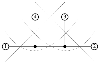
Figure 3: The medial graph (dotted) for a $4$-node network (solid).

A strand of the medial graph $M$ is a maximal path in the medial graph which continues “straight” at each vertex of $M$, that is, turns neither left nor right. There is a strand starting at each stub and ending at another stub, and possibly other strands which form closed loops.

If $\mathcal{G}$ is drawn in a disk, with the nodes on the bounding circle, the strands of a medial graph are the boundaries of a cell decomposition of the disk. The cells come in two types, corresponding to vertices and faces of $\mathcal{G}$ (between two adjacent nodes there is a cell corresponding to an exterior face of $\mathcal{G}$).

A nice property of medial strands is that, for minimal graphs (see the next section), they are boundaries of the support of equilibrium potentials. Let us explain.

Lemma 4.6.

[6] Suppose $\mathcal{G}$ is minimal. Let $a,b$ be stubs connected by a medial strand. This medial strand divides the disk into two parts $U_{+},U_{-}$. Then there is an equilibrium potential $f$ (a function harmonic on $I$ and with Dirichlet boundary conditions on $\mathcal{N}$), not identically zero, with harmonic conjugate $f^{*}$ with the property that both $f$ and $f^{*}$ are identically zero on (cells in) $U_{-}$.

For an example see Figure 4. Furthermore we have

Lemma 4.7.

[6] If $G$ is minimal and $a,b$ are two stubs, let $C_{+}$ and $C_{-}$ be the two arcs of the boundary of the disk separated by $a$ and $b$. Then $a$ and $b$ are connected by a medial strand in $\mathcal{G}$ if and only if there are equilibrium potentials $f_{+}$ and $f_{-}$ and conjugates respectively $g_{+},g_{-}$ such that $f_{+},g_{+}$ are zero on nodes and exterior faces of $C_{+}$, and $f_{-},g_{-}$ are zero on nodes and exterior faces of $C_{-}$.

Figure 4: A network (solid) with a strand (dashed) and an equilibrium potential and dual which are zero on one side. In this example all conductances are $1$.

4.4.2 Minimality and electrical transformations

A circular planar network is said to be minimal if the medial strands have the properties

1. There are no closed loops.

2. A strand does not intersect itself.

3. No two strands intersect more than once.

The reason we define minimal graphs is that every circular planar network is equivalent, in the sense of having the same response matrix, to a minimal circular planar network. Moreover minimal graphs are precisely those in which the reconstruction has a unique solution [6].

In [7] it was shown that any circular planar network can be converted into a minimal circular planar network by a sequence of local transformations called electrical transformations. An electrical transformation is a local rearrangement of the graph and conductances of one of the types shown in Figure 5. They consist of:

1. Removing a “dead branch” (remove a non-node vertex of degree $1$ and the edge connecting it to the rest of the graph) or a self-loop.

2. Replacing two conductors $c_{1},c_{2}$ in series with a single conductor of conductance $\frac{c_{1}c_{2}}{c_{1}+c_{2}}$ (as long as the common vertex is not a node).

3. Replacing parallel edges of conductances $c_{1},c_{2}$ with a single edge of conductance $c_{1}+c_{2}$.

4. the “Y-Delta” move, also called star-triangle move: an internal vertex of degree three with edges of conductance $c_{1},c_{2},c_{3}$ is replaced by a triangle with edges of conductance $\frac{c_{1}c_{2}}{c_{1}+c_{2}+c_{3}},\frac{c_{1}c_{3}}{c_{1}+c_{2}+c_{3}},\frac{c_{2}c_{3}}{c_{1}+c_{2}+c_{3}}$ as in the diagram.

The reverse of a Y-Delta move is a Delta-Y move and is also allowed. The inverse transformation takes conductances $c_{1},c_{2},c_{3}$ on the “Delta” to conductances

$$\frac{c_{1}c_{2}+c_{1}c_{3}+c_{2}c_{3}}{c_{1}},\frac{c_{1}c_{2}+c_{1}c_{3}+c_{2}c_{3}}{c_{2}},\frac{c_{1}c_{2}+c_{1}c_{3}+c_{2}c_{3}}{c_{3}}$$

on the Y. For simplicity when we say “Y-Delta move” we mean either a Y-Delta or its reverse.

Figure 5: The electrical transformations.

We say that circular planar networks $\mathcal{G},\mathcal{G}^{\prime}$ on the same number of nodes are topologically equivalent if one can be converted to the other as graphs (that is, ignoring conductances), using electrical transformations. We define circular planar networks $\mathcal{G},\mathcal{G}^{\prime}$ to be electrically equivalent if they have the same response matrix.

4.4.3 Topological equivalence

It is not hard to show that any circular planar network is topologically equivalent to a minimal circular planar network, that is, can be converted to a minimal network by electrical transformations. The idea is to simply chart how the moves act on medial strands: Each of the first three types of moves decreases the number of crossings of the medial strands (that is, the number of edges of the network). We isotope the strands, leaving their endpoints fixed, until each strand has no self-intersections and crosses each other strand at most once. During this isotopy, each time a strand crosses an intersection of other strands we perform a Y-Delta move on the graph; other singularities encountered will decrease the number of crossings and so are finite in number.

This argument shows that for the purposes of determining topological equivalence one can assume $\mathcal{G}$ and $\mathcal{G}^{\prime}$ are minimal. What is a bit harder to show is that the “minimization” process leads to a unique minimal graph, up to Y-Delta moves. That is, if $\mathcal{G}^{\prime}$ and $\mathcal{G}^{\prime\prime}$ are minimal graphs obtained from the same graph $\mathcal{G}$ then $\mathcal{G}^{\prime}$ can be converted to $\mathcal{G}^{\prime\prime}$ using only Y-Delta moves (and Delta-Y moves). See Theorem 4.8 below.

For a given minimal circular planar graph $\mathcal{G}$ with $n$ nodes, the medial graph has $2n$ stubs, one starting to the left and right of each node. The medial paths connect these stubs in pairs. Let $\pi$ denote the pairing of the stubs by the medial paths; if we label the stubs from $1$ to $2n$ in cclw order then we can think of $\pi$ as a fixed-point free involution of $\{1,2,\dots,2n\}$.

Theorem 4.8 ([6]).

Two minimal graphs $\mathcal{G},\mathcal{G}^{\prime}$ are topologically equivalent if and only if they have the same medial strand stub involution.

Proof.

If two minimal graphs have the same medial strand involution then one can isotope the strands without forming any new crossings so the two graphs are isomorphic: for example put the nodes and stubs in general position on a circle respecting their circular order; now isotope the strands to straight chords across the disk.

Conversely, by Lemma 4.7 the response matrix of a minimal graph $\mathcal{G}$ determines its stub involution, since the supports of equilibrium potentials and their harmonic conjugates are determined by $L$. ∎

4.4.4 Well-connected and non-well-connected networks

Recall that a network is well-connected if all non-interlaced minors of $L$ are strictly positive. Equivalently, for any non-interlaced subsets of nodes $A,B$, there is a grove connecting points of $A$ to those of $B$ in pairs. (If $|A|=|B|=k$ one can just look for a set of $k$ pairwise disjoint paths connecting points of $A$ to those of $B$; such a set is easily completed to a grove by adding extra edges.)

What stub involution corresponds to a well-connected network? It is not hard to construct well-connected graphs. One nice family is illustrated in Figure 6.

Figure 6: The standard networks $\Gamma_{k}$ for $k=2,\dots,6$. These are well-connected.

We leave it to the reader to show that these graphs are well-connected, and have stub involution $\pi_{\text{well}}$ which pairs $i$ with $n+i$ for each $i$. That is, each stub is paired with the diametrically opposite stub.

Corollary 4.9.

For a minimal graph $\mathcal{G}$ on $n$ nodes, the following are equivalent:

1. $\mathcal{G}$ is well-connected.

2. Its stub involution is $\pi_{\text{well}}$.

3. $\mathcal{G}$ is topologically equivalent to $\Gamma_{n}$.

Another nice family of well-connected graphs which are in addition circularly symmetric (for $n$ odd) and nearly circularly symmetric (for $n$ even) is given in Figure 7. See Figure 8 for a third family.

Figure 7: Some (almost) circularly symmetric well-connected graphs.

Figure 8: A different family of well-connected graphs for even $n$.

What about non-well connected graphs? Is there any structure to the set of topological equivalence classes of $n$-node networks? See below.

4.4.5 Electrical equivalence

We discussed topological equivalence above. Regarding electrical equivalence, we have

Theorem 4.10.

Electrical transformations do not change the response matrix.

Proof.

It suffices to show that electrical transformations preserve current flow. More precisely, the current flow on the “before” network will be equal to the current flow on the “after” network if defined appropriately on any added edges.

This is clear for transformations of type $1$ (removing a dead branch or self-loop) since these edges have no current flow. For a type $3$ move (parallel reduction) the current flow on $c_{1}$ is $c_{1}df(e)$ where $f$ is the corresponding potential on the vertices. Similarly the current flow across $c_{2}$ is $c_{2}df(e)$. The current flow on the combined edge is $(c_{1}+c_{2})df(e)$ which is the sum of the current flows on the individual edges.

For a type $2$ (series) transformation, the relevant equation is $c_{1}df(e_{1})=c_{2}df(e_{2})$ since no current is lost at the center vertex. This implies that

$$c_{1}df(e_{1})=\frac{c_{1}c_{2}}{c_{1}+c_{2}}(df(e_{1})+df(e_{2})),$$

and $df(e_{1})+df(e_{2})$ is the potential drop across the combined edges.

A similar computation works for the Y-Delta move. When converting from a Y to a Delta, the current along the edges of the Y directed towards the central vertex is $c_{1}df_{1},c_{2}df_{2},c_{3}df_{3}$ (where the $df_{i}$ are the potential drops) which must add to zero since no current is lost at the central vertex:

$$c_{1}df_{1}+c_{2}df_{2}+c_{3}df_{3}=0.$$

A short computation then shows that

$$c_{1}df_{1} = C_{12}(df_{1}-df_{2})+C_{13}(df_{1}-df_{3}),$$

$$c_{2}df_{2} = C_{12}(df_{1}-df_{2})+C_{13}(df_{1}-df_{3}),$$

$$c_{3}df_{3} = C_{12}(df_{1}-df_{2})+C_{13}(df_{1}-df_{3})$$

for arbitrary $df_{1},df_{2},df_{2}$ when and only when $C_{ij}=\frac{c_{i}c_{j}}{c_{1}+c_{2}+c_{3}}$. ∎

As a consequence of this theorem, for determining the space of response matrices of planar networks we need only consider minimal networks.

4.5 Reconstruction and the space of networks

Given a matrix which satisfies the conditions and inequalities of Theorem (4.1), is it the response matrix of a circular planar network? How can one determine the conductances from $L$? This is the Reconstruction Problem or EIT problem. It is closely related to the Electrical Equivalence Problem: what sets of minimal networks are electrically equivalent?

4.5.1 Algorithm

Both [8] and [6] gave an iterative algorithm for reconstruction on any minimal graph. The idea is as follows. Any network is equivalent to one which has either an edge connecting adjacent nodes or a node of degree $1$ (take a strand $ab$ with the property that there are no strands completely contained on one side $U_{+}$ of it; using Y-Delta moves, move all crossings in $U_{+}$ of other strands to the other side $U_{-}$. The node adjacent to $a$ and inside $U_{+}$ will either have degree $1$ or be connected to its adjacent node on the other side of $a$).

One can now compute the conductance on this edge $e$ from $L$: find the potential with values zero on side $U_{+}$ of strand $ab$. Then the conductance $c_{e}$ is easily obtained from the current.

Removing the edge $e$ (if it connected nodes) or contracting the edge $e$ (if it is adjacent to a degree-$1$ node) results in a new network which is still minimal, and the new response matrix is a simple rational function of the old response matrix.

This algorithm shows that the conductances are rational functions of the $L_{ij}$. However it is not so easy to use this to give an explicit formula for the conductances as a function of the response matrix. In [20] an explicit formula is given for the reconstruction problem for the standard graphs $\Gamma_{n}$ of Figure 6, which expresses $c_{e}$ as a ratio of polynomials in the $L_{ij}$ which are Pfaffians of skew-symmetric matrices formed from $L$. This can be considered in some sense the best possible result for $\Gamma_{n}$ since the polynomials of the $L_{ij}$ are shown there to be irreducible in general. However this does not preclude the possibility that for other well-connected networks there is a simpler formula: see [21].

4.5.2 Partial order on networks

By allowing some conductances to go to zero and others to tend to $\infty$ a network degenerates (topologically, we remove edges of conductance zero and contract edges of conductance $\infty$).

There is a partial order on networks under this degeneration. We define $\mathcal{G}\leq\mathcal{G}^{\prime}$ if a network equivalent to $\mathcal{G}$ can be obtained from a network equivalent to $\mathcal{G}^{\prime}$ by contraction and deletion of edges.

One can show that every minimal network is a minor (in the sense of contraction and/or deletion of edges) of a well-connected network. So the well-connected network is the unique maximal element in this partial order. If we allow disconnected networks, the networks which are minimal are those whose stub involution is a non-crossing matching; see Figure 10.

Lemma 4.11.

If $\mathcal{G},\mathcal{G}^{\prime}$ are minimal circular planar networks and $\mathcal{G}\leq\mathcal{G}^{\prime}$ then there is a sequence $\mathcal{G}_{1}\leq\mathcal{G}_{2}\leq\dots\leq\mathcal{G}_{k}=\mathcal{G}^{\prime}$ of minimal networks where $\mathcal{G}_{1}$ is equivalent to $\mathcal{G}$ and $\mathcal{G}_{i}$ is obtained from a network equivalent to $\mathcal{G}_{i+1}$ by deletion or contraction of a single edge.

Proof.

First suppose that $\mathcal{G}$ is obtained from $\mathcal{G}^{\prime}$ by deleting a single edge $e$ (the case of contraction is equivalent by duality). Here is how one minimizes the resulting network: let $a,b,c,d$ in cclw order be the stubs of the strands $ac$ and $bd$ crossing at edge $e$. Let $U_{1},U_{2},U_{3},U_{4}$ be the four arcs of the circle separated by $a,b,c,d$, so that $U_{1}$ is the arc from $a$ to $b$, etc. Using Y-Delta moves we can first comb strands so that strands connecting stubs from $U_{1}$ to $U_{3}$ cross “left” of $e$, that is, do not enter the region delimited by the path $bec$, and strands connecting stubs from $U_{2}$ and $U_{4}$ cross “below” $e$, that is, do not enter the region delimited by the path $ced$. See the Figure 9. Now we resolve the crossing at $e$, creating a strand connecting $a$ and $b$ and another connecting $c$ and $d$. The strand $ab$ forms a bigon with any strand from $U_{2}$ to $U_{4}$. To minimize the resulting network we resolve all crossings of these strands with the semi-strand from $b$ to $e$ as indicated in Figure 9. The resulting network is now minimized (and any minimization results in a network equivalent to this one).

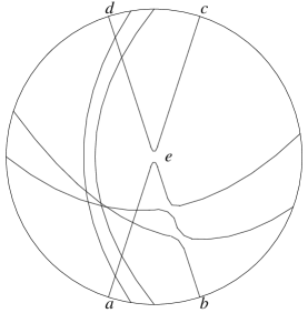
Figure 9: When a conductance $e$ goes to zero, comb strands left and down (left figure); then resolve strand crossings between $b$ and $e$ (right figure).

If we perform this sequence of resolutions in order of the crossings along the semistrand $be$ from the boundary towards the center, (resolving the crossing at $e$ last) the intermediate networks are all minimal. This completes the proof in the case when $\mathcal{G}$ is obtained from $\mathcal{G}^{\prime}$ by resolution of a single crossing.

In the general case, we contract and delete multiple edges of $\mathcal{G}^{\prime}$, then minimize to get $\mathcal{G}$. Take a path in the space of conductances which sends the desired conductances to zero or infinity, one after another, in any order. Let $L(t)$ be the corresponding path in the space of response matrices. When we minimize the resolution of a single crossing as above, the resulting $L$ matrix does not change (in the sense that no additional minors become zero), since minimization leaves $L$ invariant. Thus the sequence of resolutions is replaced with a sequence of “minimal” resolutions, that is, resolutions which preserve minimality. ∎

This partial order on networks induces a partial order on fixed-point free involutions of $\{1,\dots,2n\}$. This partial order is graded by the number of crossings in the involution, that is, the number of pairs $i<j<k<\ell$ with $i$ paired with $k$ and $j$ paired with $\ell$. Moving one level down in the partial order corresponds to resolving exactly one crossing which is adjacent to the boundary (in the sense that there is a path in the disk from the crossing to the boundary circle which does not meet any strand). Algebraically, moving up one level corresponds to the operation of conjugating the involution by a transposition in such a way as to increase the number of crossings by $1$.

See Figure 10 for the Hasse diagram of the partial order in the case $n=3$.

Figure 10: The partial order on circular planar networks with three nodes. Only the medial graphs are shown.

This partial order describes the cell structure of the space of networks.

4.5.3 Minimal sets of inequalities

What is the structure of the set of response matrices of all circular planar networks? The set $\Omega$ of response matrices of circular planar networks on $n$ nodes is a closed subset of $\mathbb{R}^{n(n-1)/2}$ if we use the coordinates $\{L_{ij}\}_{n\geq i>j\geq 1}.$ It is a semi-algebraic set, that is, defined by a set of algebraic inequalities $\det L_{A}^{B}\geq 0$ for the non-interlaced subsets $A,B$ of nodes. Its interior $\Omega^{+}$ is defined by using strict inequalities, and corresponds to the well-connected networks.

The number of inequalities defining $\Omega$ is exponential in $n$. However there is a smaller set of $n(n-1)/2$ inequalities which defines $\Omega^{+}$. See below.

If we consider a topological equivalence class (defined by a stub involution $\pi$) of graphs, the response matrices of networks supported on these graphs form a subset $\Omega_{\pi}\subset\Omega$, which is a subset of the boundary of $\Omega$ if $\pi\neq\pi_{\text{well}}$. $\Omega$ has the structure of a cell-complex, in which the $\Omega_{\pi}$ are the cells, see Lam and Pylyavskyy [23]. Is each cell of dimension $k$ defined by $k$ minor inequalities (and $n(n-1)/2-k$ equalities)? The answer is probably yes, but at the moment our understanding is limited. A similar situation where the cell structure is explicitly worked out is Postnikov [29] who deals with totally positive/totally nonnegative matrices and the totally nonnegative Grassmannian.

Let us discuss here only the minimal sets of inequalities defining the set $\Omega^{+}$. Somewhat remarkably, there are many different sets $\begin{pmatrix}n\\ 2\end{pmatrix}$ minor determinants of $L$ whose positivity implies the positivity of all non-interlaced minors. The situation resembles that of a cluster algebra but so far we have been unable to find the relevant cluster structure.

One easy-to-remember set of $\begin{pmatrix}n\\ 2\end{pmatrix}$ minors are the central minors, defined as follows. Suppose first $n$ is odd. Define $M_{i,1}$ for $1\leq i\leq(n-1)/2$ to be the minor $L_{A}^{B}$ with $A=\{1,2,\dots,i\}$ and $B=\{(n-1)/2+1,(n-1)/2+2,\dots,(n-1)/2+i\}$. Let $M_{i,j}$ be the minor obtained from $M_{i,1}$ by rotating the indices cyclically by $j-1$, so that $A=\{j,j+1,\dots,j+i\}$ and likewise for $B$.

These minors are called central minors since, if we arrange the $n$ points evenly spaced on a circle, and connect each element of $A$ to the corresponding point of $B$ opposite it, we get a set of $i$ parallel chords which are “central” in the sense that they are as close to a fixed diagonal of the circle as possible while remaining disjoint from each other. See Figure 11 for an example.

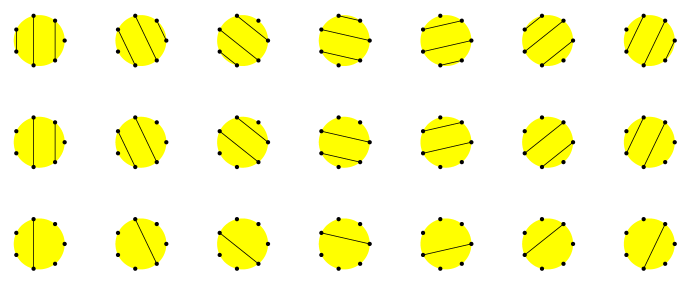
Figure 11: The $21$ central minors for a well-connected network on $7$ nodes.

In the case $n$ is even we modify the above; define $M_{i,j}$ for $i$ even as before, but for $i$ odd we have, for each diagonal, two choices of positioning of the chords to make them “most central”; choose one of these arbitrarily. These “off-center” minors are part of our set of central minors. See Figure 12 for a natural choice.

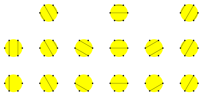
Figure 12: The $15$ central minors for a well-connected network on $6$ nodes.

Theorem 4.12 ([21]).

If the central minors $\{M_{i,j}\}$ are positive then all noninterlaced minors are positive.

The following proof is lifted directly from [21].

Proof.

This follows using two identities for minors.

Let $U$ be a matrix, and let $a,b,c$ index some of its columns, and $z,d$ index some of its rows. Then it is elementary that

$$0=\begin{vmatrix}U_{z,a}&U_{z,b}&U_{z,c}\\ U_{z,a}&U_{z,b}&U_{z,c}\\ U_{d,a}&U_{d,b}&U_{d,c}\\ \end{vmatrix}=U_{z,a}\begin{vmatrix}U_{z,b}&U_{z,c}\\ U_{d,b}&U_{d,c}\\ \end{vmatrix}-U_{z,b}\begin{vmatrix}U_{z,a}&U_{z,c}\\ U_{d,a}&U_{d,c}\\ \end{vmatrix}+U_{z,c}\begin{vmatrix}U_{z,a}&U_{z,b}\\ U_{d,a}&U_{d,b}\\ \end{vmatrix}.$$

Suppose $U$ is invertible, and let $M$ denote its inverse. Let $r_{1},\dots,r_{k}$ denote the row indices of $M$ (and column indices of $U$), and $c_{1},\dots,c_{k}$ denote the column indices of $M$ (and row indices of $U$). Dividing through by $(\det U)^{2}$ and using Jacobi’s identity relating minors of a matrix to minors of its inverse, we obtain

$$0=\det(M_{i,j})^{i\neq a}_{j\neq z}\det(M_{i,j})^{i\neq b,c}_{j\neq z,d}-\det(M_{i,j})^{i\neq b}_{j\neq z}\det(M_{i,j})^{i\neq a,c}_{j\neq z,d}+\det(M_{i,j})^{i\neq c}_{j\neq z}\det(M_{i,j})^{i\neq a,b}_{j\neq z,d}.$$

Since the column $z$ is always excluded, we may as well suppose that $M$ is a $k\times(k-1)$ matrix. Then

$$\det(M_{i,j})^{i\neq b}_{j}\det(M_{i,j})^{i\neq a,c}_{j\neq d}=\det(M_{i,j})^{i\neq a}_{j}\det(M_{i,j})^{i\neq b,c}_{j\neq d}+\det(M_{i,j})^{i\neq c}_{j}\det(M_{i,j})^{i\neq a,b}_{j\neq d}.$$

For example, taking $M=L^{9,8,7,6,5}_{1,2,3,4}$ and $a,b,c,d=9,8,5,4$, we have

$$\Big{|}L^{9,7,6,5}_{1,2,3,4}\Big{|}=\frac{\Big{|}L^{8,7,6,5}_{1,2,3,4}\Big{|}\,\Big{|}L^{9,7,6}_{1,2,3}\Big{|}+\Big{|}L^{9,8,7,6}_{1,2,3,4}\Big{|}\,\Big{|}L^{7,6,5}_{1,2,3}\Big{|}}{\Big{|}L^{8,7,6}_{1,2,3}\Big{|}}.$$

We can denote this pictorially as

$$\raisebox{-14.05249pt}{\mbox{\hskip 2.0pt}\phantom{\rule{34.12749pt}{37.13875pt}}\hskip 2.0pt}=\frac{\raisebox{-14.05249pt}{\mbox{\hskip 2.0pt}\phantom{\rule{34.12749pt}{37.13875pt}}\hskip 2.0pt}\raisebox{-14.05249pt}{\mbox{\hskip 2.0pt}\phantom{\rule{34.12749pt}{37.13875pt}}\hskip 2.0pt}+\raisebox{-14.05249pt}{\mbox{\hskip 2.0pt}\phantom{\rule{34.12749pt}{37.13875pt}}\hskip 2.0pt}\raisebox{-14.05249pt}{\mbox{\hskip 2.0pt}\phantom{\rule{34.12749pt}{37.13875pt}}\hskip 2.0pt}}{\raisebox{-14.05249pt}{\mbox{\hskip 2.0pt}\phantom{\rule{34.12749pt}{37.13875pt}}\hskip 2.0pt}}.$$

We call transformations of this type the “jaw move”.

For a given non-interleaved determinant interspersed with at least one isolated node, we can take $b$ to be one of the interspersed isolated nodes, and $a$ and $c$ to be the first and last of the nodes on the same side as $b$, and $d$ to be either first or last node on the other side as $b$. With this choice of $a,b,c,d$, the jaw move expresses the original determinant as a positive rational function of “simpler” non-interleaved determinants, where a determinant is simpler if it has fewer strands, or else the same number of strands but fewer interspersed isolated nodes.

By repeated application of the jaw rule, any non-interleaved determinant can be expressed as a positive rational function of non-interleaved contiguous determinants.

The other identity that we need is based on Dodgson condensation (and is also called the Desnanot-Jacobi identity). It can be derived in a similar way as the jaw move, with the elementary starting identity

$$U_{c,a}U_{d,b}=\begin{vmatrix}U_{c,a}&U_{c,b}\\ U_{d,a}&U_{d,b}\\ \end{vmatrix}+U_{c,b}U_{d,a}.$$

Dividing through by $(\det U)^{2}$ and using Jacobi’s identity, we obtain

$$\det(M_{i,j})^{i\neq a}_{j\neq c}\det(M_{i,j})^{i\neq b}_{j\neq d}=\det(M_{i,j})^{i}_{j}\det(M_{i,j})^{i\neq a,b}_{j\neq c,d}+\det(M_{i,j})^{i\neq b}_{j\neq c}\det(M_{i,j})^{i\neq a}_{j\neq d}.$$

For example, taking $M=L^{8,7,6}_{1,2,3}$ and $a,b,c,d=8,6,3,1$, we obtain

$$\Big{|}L^{8,7}_{1,2}\Big{|}=\frac{\Big{|}L^{8,7,6}_{1,2,3}\Big{|}\,\Big{|}L^{7}_{2}\Big{|}+\Big{|}L^{7,6}_{1,2}\Big{|}\,\Big{|}L^{8,7}_{2,3}\Big{|}}{\Big{|}L^{7,6}_{2,3}\Big{|}}.$$

which we can denote pictorially as

$$\raisebox{-14.05249pt}{\mbox{\hskip 2.0pt}\phantom{\rule{34.12749pt}{37.13875pt}}\hskip 2.0pt}=\frac{\raisebox{-14.05249pt}{\mbox{\hskip 2.0pt}\phantom{\rule{34.12749pt}{37.13875pt}}\hskip 2.0pt}\raisebox{-14.05249pt}{\mbox{\hskip 2.0pt}\phantom{\rule{34.12749pt}{37.13875pt}}\hskip 2.0pt}+\raisebox{-14.05249pt}{\mbox{\hskip 2.0pt}\phantom{\rule{34.12749pt}{37.13875pt}}\hskip 2.0pt}\raisebox{-14.05249pt}{\mbox{\hskip 2.0pt}\phantom{\rule{34.12749pt}{37.13875pt}}\hskip 2.0pt}}{\raisebox{-14.05249pt}{\mbox{\hskip 2.0pt}\phantom{\rule{34.12749pt}{37.13875pt}}\hskip 2.0pt}}.$$

We call transformations of this type the “condensation move”.

If both sides of the determinant are contiguous, but the crossings are off-center, then we can pick $a$ and $d$ to be the paired nodes that are most off-center, and $b$ and $c$ to be the nodes next to the crossing but not in the crossing (and closer to the center). Then after a condensation move, the original determinant is expressed as a positive rational function of contiguous crossings that are strictly more central. By repeated application of such condensation moves, any contiguous determination may be expressed as a positive rational function of central contiguous crossings.

The remaining case to check is for $n$ even, with the (minimally) off-center contiguous crossings come in pairs, of which only one is included in the base cluster. Using a condensation move we can express a minimally off-center contiguous crossing in terms of its opposite minimally off-center contiguous crossing and central contiguous crossings as shown below

$$\raisebox{-14.05249pt}{\mbox{\hskip 2.0pt}\phantom{\rule{34.12749pt}{37.13875pt}}\hskip 2.0pt}=\frac{\raisebox{-14.05249pt}{\mbox{\hskip 2.0pt}\phantom{\rule{34.12749pt}{37.13875pt}}\hskip 2.0pt}\ \raisebox{-14.05249pt}{\mbox{\hskip 2.0pt}\phantom{\rule{34.12749pt}{37.13875pt}}\hskip 2.0pt}+\raisebox{-14.05249pt}{\mbox{\hskip 2.0pt}\phantom{\rule{34.12749pt}{37.13875pt}}\hskip 2.0pt}\ \raisebox{-14.05249pt}{\mbox{\hskip 2.0pt}\phantom{\rule{34.12749pt}{37.13875pt}}\hskip 2.0pt}}{\raisebox{-14.05249pt}{\mbox{\hskip 2.0pt}\phantom{\rule{34.12749pt}{37.13875pt}}\hskip 2.0pt}}$$

∎

4.6 The Jacobian

A remarkable property of the birational map from conductances to the (appropriate set of) $L$ matrix minors for minimal networks is that the Jacobian is $\pm 1$:

Theorem 4.13 ([21]).

$$\det\left(\frac{\partial\log M_{i}}{\partial\log c_{j}}\right)=\pm 1.$$

In other words the volume form $\prod_{e}\frac{dc_{e}}{c_{e}}$ on the space of conductances is mapped to $\pm 1$ times the volume form $\prod_{i}\frac{dM_{i}}{M_{i}}$ on the space of $L$-matrix minors. Note that the matrix entries have a probabilistic interpretation: each $M_{i}$ can be written $M_{i}=\mathrm{Pr}(\pi)/\mathrm{Pr}(\text{unc})$ for some noninterlaced pairing $\pi$. Thus

$$\frac{\partial\log M_{i}}{\partial\log c_{j}}=\frac{c_{j}}{Z(\pi)}\frac{\partial Z(\pi)}{\partial c_{j}}-\frac{c_{j}}{Z_{\mathrm{unc}}}\frac{\partial Z_{\mathrm{unc}}}{\partial c_{j}}$$

is the difference in the probability that edge $e_{j}$ is in a random $\pi$-pairing, minus the probability that $e_{j}$ is in a random uncrossing.

The proof of this theorem relies of techniques developed in [29] and [30] and is too long to give here. Let us just give an example, for a well-connected network on $3$ nodes, the Y of Figure 1. The central minors in terms of the conductances are $L_{ij}=\frac{c_{i}c_{j}}{c_{1}+c_{2}+c_{3}}.$ The above Jacobian matrix (with columns in the order $L_{12},L_{13},L_{23}$) is

$$\begin{pmatrix}1-\frac{1}{c_{1}+c_{2}+c_{3}}&1-\frac{1}{c_{1}+c_{2}+c_{3}}&-\frac{1}{c_{1}+c_{2}+c_{3}}\\ 1-\frac{1}{c_{1}+c_{2}+c_{3}}&-\frac{1}{c_{1}+c_{2}+c_{3}}&1-\frac{1}{c_{1}+c_{2}+c_{3}}\\ -\frac{1}{c_{1}+c_{2}+c_{3}}&1-\frac{1}{c_{1}+c_{2}+c_{3}}&1-\frac{1}{c_{1}+c_{2}+c_{3}}\\ \end{pmatrix}$$

whose determinant is $1$.

5 Networks on surfaces with nontrivial topology

Some of the material in the preceding section on circular planar networks has been extended to the case of annular networks and more generally networks on surfaces. However the theory is not as complete at present as in the case of circular planar graphs. Moreover beyond the annulus and torus the theory is for the most part nonexistent.

We can nonetheless ask the same questions as arose in the planar case:

1. What is the natural notion of response matrix?

2. For which networks can we reconstruct the conductances from the response matrix?

3. What is the structure of the space of response matrices?

4. What natural combinatorial objects are relevant?

Our answers, briefly, are as follows. We elaborate on these in the following sections.

1. We use (the Schur reduction of) the bundle Laplacian for a flat $\mathbb{C}^{*}$-connection or a flat $\text{SL}_{2}(\mathbb{C})$-connection on the network.

2. We can conjecturally reconstruct conductances for minimal networks on the annulus. For other surfaces reconstruction is not in general possible, unless we are given more data: we (conjecturally) need to provide “spectral” data as well.

3. We don’t know what the structure of the space of response matrices is, even for the annulus. However we have a description in the case when there are no nodes, for the annulus and torus.

4. The natural combinatorial objects are “cycle-rooted spanning forests”: forests in which each component has a unique (topologically nontrivial) cycle.

5.1 Vector bundle Laplacian

In the case of a network on a surface it is natural to consider not the standard Laplacian but a more general Laplacian operator, the vector bundle Laplacian, which depends on a connection on the bundle (see definitions below). This is because the standard Laplacian does not contain very much information about the topology of the surface on which the network is embedded…in particular the reconstruction problem is not solvable in general (as an example consider the network on an annulus with two vertices, both nodes, and two edges joining them with different homotopy classes). From the bundle Laplacian we construct a response matrix which contains more information than the one constructed from the standard Laplacian, and conjecturally allows reconstruction for minimal networks.

Let us first define vector bundles and connections on a network.

5.1.1 Vector bundles and connections

Given a fixed vector space $W$, a $W$-bundle, or simply a vector bundle on a network $\mathcal{G}$ is the choice of a vector space $W_{v}$ isomorphic to $W$ for every vertex $v$ of $\mathcal{G}$. A vector bundle can be identified with the vector space $W_{\mathcal{G}}:=\oplus_{v}W_{v}\cong W^{|\mathcal{G}|}$, called the total space of the bundle. A section of a vector bundle is an element of $W_{\mathcal{G}}$.

A connection $\Phi$ on a $W$-bundle is the choice for each edge $e=vv^{\prime}$ of $\mathcal{G}$ of an isomorphism $\phi_{vv^{\prime}}$ between the corresponding vector spaces $\phi_{vv^{\prime}}:W_{v}\to W_{v^{\prime}}$, with the property that $\phi_{vv^{\prime}}=\phi_{v^{\prime}v}^{-1}$. This isomorphism is called the parallel transport of vectors in $W_{v}$ to vectors in $W_{v^{\prime}}$. Two connections $\Phi,\Phi^{\prime}$ are said to be gauge equivalent if there is for each vertex an isomorphism $\psi_{v}:W_{v}\to W_{v}$ such that the diagram

$$\begin{CD}W_{v}@>{\phi_{vv^{\prime}}}>{}>W_{v^{\prime}}\\ @V{}V{\psi_{v}}V@V{}V{\psi_{v^{\prime}}}V\\ W_{v}@>{\phi^{\prime}_{vv^{\prime}}}>{}>W_{v^{\prime}}\end{CD}$$

commutes. In other words $\Phi^{\prime}$ is just a base change of $\Phi$. Note that the connection has nothing to do with the conductances.

Given an oriented cycle $\gamma$ in $\mathcal{G}$ starting at $v$, the monodromy of the connection around $\gamma$ is the element of $\text{End}(W_{v})$ which is the product of the parallel transports around $\gamma$. Monodromies starting at different vertices on $\gamma$ are conjugate, as are monodromies of gauge-equivalent connections.

A line bundle is a $W$-bundle where $W\cong\mathbb{C}$, the $1$-dimensional complex vector space. In this case given a connection if we choose a basis for each $\mathbb{C}$ then the parallel transport along an edge is just multiplication by an element of $\mathbb{C}^{*}=\mathbb{C}\setminus\{0\}$. The monodromy of a cycle is in $\mathbb{C}^{*}$ and does not depend on the starting vertex of the cycle (or gauge).

5.1.2 Flat connections

A connection on a network embedded on a surface $\Sigma$ is said to be a flat connection if the monodromy around faces of $\mathcal{G}$ is trivial. This implies that the monodromy is trivial around loops on $\mathcal{G}$ which are null-homotopic as loops on $\Sigma$.

It is not hard to see that flat connections, modulo gauge equivalence, are in bijection with homomorphisms of $\pi_{1}(\Sigma)$ into the group of automorphisms of $W$.

5.1.3 The Laplacian

The Laplacian $\Delta$ on a $W$-bundle with connection $\Phi$ is the linear operator $\Delta:W_{\mathcal{G}}\to W_{\mathcal{G}}$ defined by

$$\Delta f(v)=\sum_{v^{\prime}\sim v}c_{vv^{\prime}}(f(v)-\phi_{v^{\prime}v}f(v^{\prime}))$$

where the sum is over neighbors $v^{\prime}$ of $v$.

Note that if the vector bundle is trivial, in the sense that $\phi_{vv^{\prime}}$ is the identity for all edges, this is our the notion of graph Laplacian from (1) (or more precisely, the direct sum of $\dim W$ copies of the Laplacian).

As in the case of the standard network Laplacian we often think of $\Delta$ as a matrix $\Delta=(\Delta_{vv^{\prime}})_{v,v^{\prime}\in V}$ whose entries are $-c_{vv^{\prime}}$ times the parallel transport from $v^{\prime}$ to $v$. In particular the conductance is acting as a scalar multiplication in $W$.

Here is an example. Let $\mathcal{G}=K_{3}$ the triangle with vertices $\{v_{1},v_{2},v_{3}\}$. Let $\Phi$ be the line bundle connection with $\phi_{v_{i}v_{j}}=z_{ij}\in\mathbb{C}^{*}.$ Then in the natural basis, $\Delta$ has matrix

$$\Delta=\left(\begin{matrix}c_{12}+c_{13}&-c_{12}z_{12}&-c_{13}z_{13}\\ -c_{12}z_{12}^{-1}&c_{12}+c_{23}&-c_{23}z_{23}\\ -c_{13}z_{13}^{-1}&-c_{23}z_{23}^{-1}&c_{13}+c_{23}\end{matrix}\right).$$ (15)

5.1.4 Edge bundle

One can extend the definition of a vector bundle to the edges of $\mathcal{G}$. In this case there is a vector space $W_{e}\cong W$ for each edge $e$ as well as each vertex. One defines connection isomorphisms $\phi_{ve}=\phi_{ev}^{-1}$ for a vertex $v$ and edge $e$ containing that vertex, in such a way that if $e=vv^{\prime}$ then $\phi_{vv^{\prime}}=\phi_{ev^{\prime}}\circ\phi_{ve}$, where $\phi_{vv^{\prime}}$ is the connection on the vertex bundle.

The vertex/edge bundle can be identified with $W^{|\mathcal{G}|+|E|}=W_{\mathcal{G}}\oplus W_{E}$, where $W_{E}$ is the direct sum of the edge vector spaces.

A $1$-form (or cochain) is a function on oriented edges which is antisymmetric under changing orientation. If we fix an orientation for each edge, a $1$-form is a section of the edge bundle, that is, an element of $W^{|E|}$. We denote by $\Lambda^{1}(\mathcal{G},\Phi)$ the space of $1$-forms and $\Lambda^{0}(\mathcal{G},\Phi)$ the space of $0$-forms, that is, sections of the vertex bundle.

We define a map $d:\Lambda^{0}(\mathcal{G},\Phi)\to\Lambda^{1}(\mathcal{G},\Phi)$ by $df(e)=\phi_{ye}f(y)-\phi_{xe}f(x)$ where $e=xy$ is an oriented edge from vertex $x$ to vertex $y$. We also define an operator $d^{*}:\Lambda^{1}\to\Lambda^{0}$ as follows:

$$d^{*}\omega(v)=\sum_{e=v^{\prime}v}\phi_{ev}\omega(e)$$

where the sum is over edges containing $v$ and oriented towards $v$. Despite the notation, this operator $d^{*}$ is not a standard adjoint of $d$ unless $\phi_{ev}$ and $\phi_{ve}$ are adjoints themselves, that is, if parallel transports are unitary operators (see below).

The Laplacian $\Delta$ on $\Lambda^{0}$ can then be defined as the operator $\Delta=d^{*}{\mathcal{C}}d$ as before:

$$d^{*}{\cal C}df(v) = \sum_{e=v^{\prime}v}c_{e}\phi_{ev}df(e)$$

$$= \sum_{e=v^{\prime}v}c_{e}\phi_{ev}(\phi_{ve}f(v)-\phi_{v^{\prime}e}f(v^{\prime}))$$

$$= \sum_{v^{\prime}}c_{vv^{\prime}}(f(v)-\phi_{v^{\prime}v}f(v^{\prime}))$$

$$= \Delta f(v).$$

We can see from the example (15) above on $K_{3}$ that $\Delta$ is not necessarily self-adjoint. However if $\phi_{vv^{\prime}}$ is unitary: $\phi_{vv^{\prime}}^{-1}=\phi_{v^{\prime}v}^{*}$ then $d^{*}$ will be the adjoint of $d$ for the standard Hermitian inner products on $W^{|\mathcal{G}|}$ and $W^{|E|}$, and so in this case $\Delta$ is a Hermitian, positive semidefinite operator. In particular on a line bundle if $|\phi_{vv^{\prime}}|=1$ for all edges $e=vv^{\prime}$ then $\Delta$ is Hermitian and positive semidefinite.

5.2 Minimal networks

Here we show that any network on a surface can be “minimized”, that is, made into a minimal network.

While reconstruction is not possible in general even for minimal networks (see Theorem 7.3 below), the case of the torus teaches us that the map from conductances to the reponse matrix has potentially interesting preimage.

A network $\mathcal{G}$ on a surface $\Sigma$ is minimal if, when lift to the universal cover of $\Sigma$, the network is minimal, that is, the lifts of the medial strands do not self-intersect and no two lifts intersect more than once.

As an example, see Figure 20 below.

Theorem 5.1.

Every network is topologically equivalent to a minimal network.

Proof.

Any surface with a boundary (or closed surface of genus $\geq 2$) has a hyperbolic metric (that is, a Riemannian metric of constant curvature $-1$) since its universal cover is the Poincaré disk.

Using this metric we can isotope the strands, fixing the endpoints, using a curve-shortening flow until all strands become hyperbolic geodesics. Through this isotopy each singularity encountered either reduces the number of crossings or is a triple crossing, which corresponds to a Y-Delta move of the network. In the end strands which touch the boundary will have the property that, when lifted to $\tilde{\Sigma}$, they meet other strands at most once. More generally, strands in different homotopy classes meet each other at most once in the universal cover.

If two or more intersecting strands with no endpoints (that is, which are closed loops on the surface) have the same homotopy class then we must be more careful since their geodesic representatives will be identical. The situation in the universal cover will resemble that of Figure 13, left, that is, we have a packet of strands which lie near the same geodesic, and other strands cross this packet transversely and exactly once each.

It remains to prove that in this situation we can replace the self-intersecting packet with a “combed” version of itself, where all strands are parallel and non-intersecting (they will still intersect the transversal strands). For this it suffices to consider the situation on an annulus in which the packet strands wind around the annulus forming closed loops, and a certain number of other strands cross this packet transversely. On the universal cover of the annulus, which is a bi-infinite strip, the situation is as on the left in Figure 13.

We consider, then, a periodic graph on a strip $\mathbb{R}\times[0,1]$ with conductances invariant under $x\mapsto x+1$. Suppose we now take $n$ large and truncate the strip, by removing everything far to the left of the origin, say left of $-n$, leaving free boundary conditions there, and removing everything to the right of $+n$, and similarly leaving free boundary conditions there. What remains is a planar graph on a rectangle $[-n,n]\times[0,1]$, and for this planar graph we can “comb out” the packet, as in Figure 13, from the left to the right, so that the strands of the packet become parallel paths, nonintersecting except just left of the right endpoint, where they may cross.

We claim that on the resulting combed finite planar graph, the conductances are nearly periodic, that is, a periodic function plus an error tending to zero as the distance to $\pm n$ increases. To see this we use the interpretation of the response matrix entries as ratios of weighted sums of spanning forests. In [24] it is proved that for fixed $i,j$ the truncation only changes $L_{i,j}$ by amounts tending to zero as $n\to\infty$. It is also shown that $L_{i,j}\to 0$ as the distance from $i$ to $j$ increases.

Take node $i$ on the top and $j$ on the bottom boundary of the strip. The numerator of the entry $L_{i,j}$ is the weighted sum of spanning trees wired at the boundary and with a component connecting $i$ and $j$ (see Theorem 4.3). We claim that for a typical tree the path from $i$ to $j$ does not get near $\pm n$ with high probability, that is, this path does not get far from $i$ or $j$. If the path extended far beyond $j$, then (letting $j+k$ denote the translate of $j$ by $k$) for large $k$ $L_{i,j+k}$ would be of the same order as $L_{i,j}$, since a local change of the long path from $i$ to $j$ would result in a path from $i$ to $j+k$. This contradicts the fact that $L_{i,j+k}$ tends to zero for large $k$.

Thus $L_{i,j}$ is a function depending less and less (as $n\to\infty$) on the conductances far from $i$ and $j$. This proves convergence of the conductances as $n\to\infty$, and the translation invariance of $L_{i,j}$ implies the translation invariance of the limiting conductances.

∎

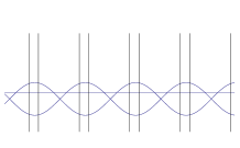
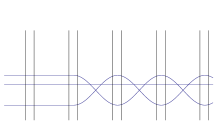
Figure 13: Combing a river with three strands.

5.3 Cycle-rooted spanning forests

Where as the standard Laplacian determinant counts spanning trees, in the case of a one- or two-dimensional vector bundle with connection the bundle Laplacian determinant counts objects called cycle-rooted spanning forests. A cycle-rooted spanning forest (CRSF) is a subset $S$ of the edges of $\mathcal{G}$, with the property that each connected component has exactly as many vertices as edges (and so has a unique cycle). See Figure 14.

Figure 14: A CRSF on a square grid.

Theorem 5.2 ([11]).

For a line bundle on a finite graph,

$$\det\Delta=\sum_{\text{CRSFs}T}\prod_{e\in T}c_{e}\prod_{\text{cycles of }T}(2-w-1/w)$$

where the sum is over all CRSFs $T$, the first product is over the edges of $T$, and the second product is over the cycles of $T$, where $w,1/w$ are the monodromies of the two orientations of the cycle.

Notice that for a line bundle the monodromies depend only on the cycle not on the starting point of the cycle.

Theorem 5.3 ([14]).

For a $\mathbb{C}^{2}$-bundle on a finite graph with $\text{SL}_{2}(\mathbb{C})$ connection, we have

$$\mathrm{qdet}\Delta=\sum_{\text{CRSFs}T}\prod_{e\in T}c_{e}\prod_{\text{cycles of }T}(2-\mathrm{Tr}(w))$$

where the sum is over all CRSFs $T$, the first product is over the edges of $T$, and the second product is over the cycles of $T$, where $w$ is the monodromy of the cycle (starting from some vertex, and in some arbitrary orientation).

Notice that the trace of the monodromy is independent of starting point (since conjugation does not change the trace) and orientation, since for a matrix $M\in\text{SL}_{2}(\mathbb{C})$, we have $\mathrm{Tr}(M)=\mathrm{Tr}(M^{-1})$.

Here the function $\mathrm{qdet}$ is the quaternion determinant of the self-dual matrix $\Delta$; this requires some explanation. A matrix $M$ with entries in ${\text{G}L}_{2}(\mathbb{C})$ is said to be self-dual if $M_{ij}=\tilde{M}_{ji}$, where

$$\widetilde{\begin{pmatrix}a&b\\ c&d\end{pmatrix}}=\begin{pmatrix}d&-b\\ -c&a\end{pmatrix}.$$

Since $\Delta_{ij}=-c_{ij}\phi_{ij}$ where $\phi_{ij}\in\text{SL}_{2}(\mathbb{C})$, we have $\Delta_{ji}=-c_{ij}\phi^{-1}_{ij}=\tilde{\Delta}_{ij}$ and so $\Delta$ is self-dual.

We define

$$\mathrm{qdet}(M)=\sum_{\sigma\in S_{n}}\text{sgn}(\sigma)\prod_{\text{cycles}}\frac{1}{2}\text{tr}(w)$$

where the sum is over the symmetric group, each permutation $\sigma$ is written as a product of disjoint cycles, and $\text{tr}(w)$ is the trace of the product of the matrix entries in that cycle. If we group together terms above with the same cycles—up to the order of traversal of each cycle—then the contribution from each of these terms is identical: reversing the orientation of a cycle does not change its trace. So we can write

$$\mathrm{qdet}(M)=\sum_{\text{cycle decomps}}(-1)^{c+n}\prod_{i=1}^{c}\widehat{\text{tr}}(w_{i}),$$

where the sum is over cycle decompositions of the indices (not taking into account the orientation of the cycles), $c$ is the number of cycles, and $w_{i}$ is the monodromy (in one direction or the other) of each cycle. Here $\widehat{\text{tr}}$ is equal to the trace for cycles of length at least $3$; cycles of length $1$ or $2$ are their own reversals so we define $\widehat{\text{tr}}(w)=\frac{1}{2}\text{tr}(w)$ for these cycles.

As an example, let $A=aI,C=cI$ and $B=\left(\begin{matrix}b_{1}&b_{2}\\ b_{3}&b_{4}\end{matrix}\right)$. Then

$$\text{Qdet}\left(\begin{matrix}A&B\\ \tilde{B}&C\end{matrix}\right)=\widehat{\text{tr}}(A)\widehat{\text{tr}}(C)-\widehat{\text{tr}}(B\tilde{B})=ac-(b_{1}b_{4}-b_{2}b_{3}).$$

Note that if $M$ is a self-dual $n\times n$ matrix then $ZM$, considered as a $2n\times 2n$ matrix is antisymmetric, where $Z$ is the matrix with diagonal blocks $\left(\begin{matrix}0&-1\\ 1&0\end{matrix}\right)$ and zeros elsewhere. The following theorem allows us to compute $Q$-determinants explicitly.

Theorem 5.4 ([9]).

Let $M$ be an $n\times n$ self-dual matrix with entries in $GL_{2}(\mathbb{C})$ and $M^{\prime}$ the associated $2n\times 2n$ matrix, obtained by replacing each entry with the $2\times 2$ block of its entries. Then $\mathrm{qdet}(M)=\mathrm{Pf}(ZM^{\prime})$, the Pfaffian of the antisymmetric matrix $ZM^{\prime}$.

Note that the matrix $\Delta^{\prime}$ (obtained by replacing entries in $\Delta$ with the $2\times 2$ block of their coefficients) is just the matrix $\Delta$ acting on the total space of the bundle $W_{\mathcal{G}}$. So up to a sign we can write

$$\mathrm{qdet}\Delta=(\det\Delta)^{1/2}.$$

5.3.1 Unitary connections and measures

In the case of a line bundle, if $\prod_{\text{cycles}}2-w-1/w\geq 0$ for every CRSF, we can define, following Theorem 5.2, a probability measure on CRSFs in which a CRSF has probability proportional to the product of its edge weights times the factor $\prod_{\text{cycles}}2-w-1/w$.

For example in the case that $|\phi_{e}|=1$ for every edge, that is, $\phi$ is a unitary connection, then $\Delta$ is a Hermitian, positive semi-definite matrix (and positive definite for generic unitary connections). In this case $|w|=1$ for all monodromies and so $2-w-1/w\geq 0$, and equal to zero only for cycles with trivial monodromy.

Similarly in the case of a two-dimensional bundle if $\phi_{e}\in\text{SU}_{2}$ for all edges then $\Delta$ is unitary and $2-\mathrm{Tr}w\geq 0$ for all monodromies.

In both cases we call $\mu=\mu_{\Phi}$ the corresponding probability measure.

Examples of natural settings of these measures are when the graphs are embedded on surfaces with geometric structures, such as a Riemannian metric (in which case the Levi-Civita connection defines parallel transport of vectors in the tangent bundle across an edge and provides a $U(1)$-connection) or an $\text{SU}_{2}$ structure on the surface and parallel transport restricted to the graph gives a $\text{SU}_{2}$ connection.

In the case of a flat connection, the monodromy of a contractible cycle is trivial, so that the probability measure is supported on CRSFs whose cycles are all topologically nontrivial. We call such CRSFs essential CRSFs.

5.4 Cycle-rooted groves

For the bundle Laplacian, the natural objects replacing groves are cycle-rooted groves. Given a graph $\mathcal{G}$ embedded on a surface with nodes $\mathcal{N}$, a cycle-rooted grove (CRG) is a collection of edges with the property that each component is either

1. A tree containing one or more nodes

2. a cycle-rooted tree containing no nodes.

Theorems 5.2 and 5.3 have an extension to the case of a graph with boundary $B\subset V$; the results are that the bundle Laplacian determinants (for the Laplacian with boundary) are weighted sums of cycle rooted groves; the weights of components with cycles are as before, and the weights of tree components are just the product of their edge weights (there is no “monodromy” contribution for tree components). See [21].

6 Annular networks

6.1 Laplacian determinant

Let $\mathcal{G}$ be a network with flat $\mathbb{C}^{*}$-connection on an annulus, and with no nodes. Let $z$ be the monodromy around a loop generating the homotopy group of the annulus. Then any simple closed loop on $\mathcal{G}$ will have monodromy $1$ if contractible, $z$ or $z^{-1}$ if noncontractible.

As a consequence by Theorem 5.2 the Laplacian determinant is

$$\det\Delta=\sum_{k=1}^{\infty}C_{k}(2-z-\frac{1}{z})^{k},$$ (16)

where $C_{k}$ is the weighted sum of CRSFs having $k$ components.

Thus $P(z)=\det\Delta$ is a Laurent polynomial in $z$ from which one can extract the information about the number of loops in a random sample of a CRSF on $\mathcal{G}$. For example substituting $x=2-z-1/z$ we have that $P(x)/P(1)$ is the probability generating function for the number of components.

Independently of the conductances, $P(z)$ contains topological information about the graph $\mathcal{G}$, for example the highest power of $z$ is the maximum number of disjoint loops which can be drawn on $\mathcal{G}$, each winding around the annulus. This is because any such set of loops can be completed to a grove by adding some edges.

There is a simple characterization of the roots of $P$. By (16) the roots come in reciprocal pairs one of which is a double root at $z=1$.

Theorem 6.1.

$P$ is reciprocal and the roots of $P$ are real, positive, and distinct except for a double root at $z=1$.

Proof.

Our first goal is to minimize the graph so that it is a string of loops as illustrated in Figure 15, each loop winding around the annulus.

As in the proof of Theorem 5.1 above, we use the curve-shortening flow on the medial strands until we have only a packet of strands winding around the core of the annulus as in Figure 13, left (but without the vertical strands). In the resulting network, choose vertices $v_{1},v_{2}$, one adjacent to each boundary and temporarily consider these to be nodes. There is one strand wrapping outside $v_{1}$ and one wrapping outside $v_{2}$. Break these strands so they have two stubs near each of $v_{1},v_{2}$. Now continue to minimize the medial strands as in the proof of Theorem 5.1. In the minimal network, the stubs from $v_{1}$ must cross to the stubs of $v_{2}$ (rather than to each other), since otherwise the network would be disconnected. We can push all intersections of the finite strands (that is, those connecting stubs) to one side of the intersections of the stub/river strands, as described in Section 6.4.1 and Figure 20 below. The network and medial graph now resemble that in Figure 16. The graph can now easily be converted into a string of loops using the sequence of operations illustrated in Figure 17.

Figure 15: Every graph on an annulus can be minimized to a string of loops.

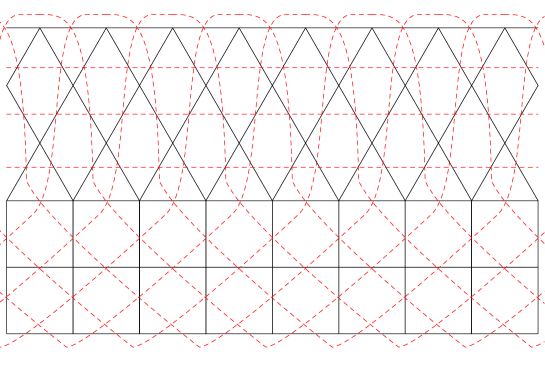
Figure 16: Intermediate stage in minimization of network on an annulus. (Medial strands dashed/red).

Figure 17: Passing from the intermediate stage to the string of loops: (1) From the network in Figure 16, use Delta-Y moves on the upper row of triangles. (1)-(2) Flatten the degree-$2$ vertices on the upper row and use Y-Deltas on the second row of vertices. (2)-(3) Use Delta-Ys on the row of triangles just above the squares. (3)-(4) Use Delta-Ys on the upper row of triangles. (4)-(5) Y-Delta. (5)-(6) Flatten and then Delta-Y. (6)-(7) Flatten.

Let $a_{1},\dots,a_{n-1}$ be the conductances on the edges of the string and $b_{1},\dots,b_{n}$ the conductances on the loops. Then the Laplacian is a tridiagonal matrix (using $X=2-z-1/z$)

$$\Delta=\begin{pmatrix}a_{1}+b_{1}X&-a_{1}&0&\\ -a_{1}&a_{1}+a_{2}+b_{2}X&-a_{2}&0&\\ 0&-a_{2}&\ddots\\ &&&a_{n-2}+a_{n-1}+b_{n-1}X&-a_{n-1}\\ &&&-a_{n-1}&a_{n-1}+b_{n}X.\end{pmatrix}$$

We pre- and post-multiply by the diagonal matrix $U$ whose diagonal entries are $b_{i}^{-1/2}$ to get

$$U\Delta U=\begin{pmatrix}\frac{a_{1}}{b_{1}}+X&\frac{-a_{1}}{\sqrt{b_{1}b_{2}}}&0&\\ \frac{-a_{1}}{\sqrt{b_{1}b_{2}}}&\frac{a_{1}}{b_{2}}+\frac{a_{2}}{b_{2}}+X&\frac{-a_{2}}{\sqrt{b_{2}b_{3}}}&0&\dots\\ 0&&\ddots\\ &&&\frac{a_{n-2}}{b_{n-1}}+\frac{a_{n-1}}{b_{n-1}}+X&\frac{-a_{n-1}}{\sqrt{b_{n-1}b_{n}}}\\ &&&\frac{-a_{n-1}}{\sqrt{b_{n-1}b_{n}}}&\frac{a_{n-1}}{b_{n}}+X.\end{pmatrix}$$

Thus we see that for each root $z$ of $P$, $-2+z+\frac{1}{z}$ is an eigenvalue of

$$M=\begin{pmatrix}\frac{a_{1}}{b_{1}}&\frac{-a_{1}}{\sqrt{b_{1}b_{2}}}&0&\\ \frac{-a_{1}}{\sqrt{b_{1}b_{2}}}&\frac{a_{1}}{b_{2}}+\frac{a_{2}}{b_{2}}&\frac{-a_{2}}{\sqrt{b_{2}b_{3}}}&0&\dots\\ 0&&\ddots\\ &&&\frac{a_{n-2}}{b_{n-1}}+\frac{a_{n-1}}{b_{n-1}}&\frac{-a_{n-1}}{\sqrt{b_{n-1}b_{n}}}\\ &&&\frac{-a_{n-1}}{\sqrt{b_{n-1}b_{n}}}&\frac{a_{n-1}}{b_{n}}.\end{pmatrix}.$$

This matrix $M$ is symmetric and so has real eigenvalues, which are positive by (16). Symmetry also implies that $M$ has orthogonal eigenvectors. Thus if $-X$ is a multiple eigenvalue of $M$ it has an eigenspace $V_{-X}$ of dimension $\geq 2$. This means there is a nonzero eigenvector of $M$ with eigenvalue $-X$ whose first coordinate is $0$. But the coordinates of an eigenvector $(x_{1},x_{2},\dots,x_{n})$ satisfy a length-three linear recurrence:

$$\lambda x_{1}=\frac{a_{1}}{b_{1}}x_{1}-\frac{a_{1}}{\sqrt{b_{1}b_{2}}}x_{2}$$

and for $i>1$

$$\lambda x_{i}=-\frac{a_{i-1}}{\sqrt{b_{i-1}b_{i}}}x_{i-1}+(\frac{a_{i-1}}{b_{i}}+\frac{a_{i}}{b_{i}})x_{i}-\frac{a_{i}}{\sqrt{b_{i}b_{i+1}}}x_{i+1}.$$

Starting from $x_{1}=0$ this implies (using that all $a_{i}\neq 0$) that $x_{i}=0$ for all $i$. This is a contradiction. We conclude that the eigenvalues of $M$, and therefore the roots of $P$, are distinct. ∎

6.2 Cylinder example

Let us compute, for a rectangular cylinder, $\det\Delta$ for the flat line bundle with monodromy $z$. This will allow us to compute the corresponding distribution of cycles in a uniform random essential CRSF. Let $H_{m,n}$ be the square grid network on a cylinder, obtained from the $n\times m$ square grid by adding edges from $(n,i)$ to $(0,i)$ for each $i\in[1,m]$. $H_{m,n}$ is a “product” of an $m$-vertex linear network $\mathcal{G}_{m}$ and a circular network $\mathbb{Z}_{n}$ of length $n$. We put a flat line bundle structure on $H_{m,n}$ by putting parallel transport $z$ on the edges $(n,i)(0,i)$ and $1$ on all other edges.

The eigenvalues of the Laplacian $\Delta_{\mathcal{G}_{m}}$ on the linear network are $2-2\cos\frac{k\pi}{m}$ for $k=1,2,\dots,m$ (the corresponding eigenvectors are $f_{k}(x)=\cos\frac{\pi k(x+1/2)}{m}$ for $x=0,1,2,\dots,m-1$).

The eigenvalues of the line-bundle Laplacian $\Delta_{\mathbb{Z}_{n}}$ on $\mathbb{Z}_{n}$ with monodromy $z$ are $2-\zeta-1/\zeta$ where $\zeta$ is an $n$th root of $z$. (The corresponding eigenvectors are $g_{k}(x)=\zeta^{x}$.) The eigenvectors on $H_{m,n}$ are the products $f_{k}g_{\ell}$ for $(k,\ell)\in[1,m]\times[0,n-1]$.

We then have

$$\det\Delta_{\Phi}=\prod_{\zeta^{n}=z}\prod_{k=1}^{m}4-2\cos\frac{k\pi}{m}-\zeta-\frac{1}{\zeta}.$$

Use the identity

$$\prod_{\zeta^{n}=z}R-\zeta-\frac{1}{\zeta}=\text{Ch}_{n}(R)$$

where $\text{Ch}_{n}$ is defined by $\text{Ch}_{n}(\alpha+\frac{1}{\alpha})=\alpha^{n}+\alpha^{-n}$ (a variant of the Chebychev polynomial).

This leads to

$$\det\Delta=(2-z-z^{-1})\prod_{k=1}^{m}(\text{Ch}_{n}(4-2\cos\frac{k\pi}{m})-z-\frac{1}{z})$$

$$=w\prod_{k=1}^{m}w+\text{Ch}_{n}(4-2\cos\frac{k\pi}{m})-2$$

where $w=2-z-\frac{1}{z}$. If we let $Q(w)$ be this polynomial then $Q(w)/Q(1)$ is the probability generating function of the number of cycles in a uniform random essential CRSF.

It is interesting to consider what happens to this distribution for a large annulus, when $m,n\to\infty$ with $m/n$ converging to a fixed quantity $\tau$. For large $n$, $\text{Ch}_{n}(4-2\cos\frac{k\pi}{m})$ is large unless $k$ is near $0$. Thus only values of $k$ near $0$ affect the limiting distribution. We have $4-2\cos\frac{k\pi}{m}=2+\frac{\pi^{2}k^{2}}{m^{2}}+O(\frac{k}{m})^{4}=\alpha_{k}+1/\alpha_{k}$ where $\alpha_{k}=1+\frac{\pi k}{m}+O(\frac{k}{m})^{2}$. Thus in the limit $m,n\to\infty$ with $m/n\to\tau$ we have $\text{Ch}_{n}(4-2\cos\frac{k\pi}{m})=2\cosh\frac{\pi k}{\tau}+o(1)$. The limit probability generating function for the number of cycles is then

$$Q(w)/Q(1)=w\prod_{k=1}^{\infty}\left(\frac{w+2\cosh\frac{\pi k}{\tau}-2}{2\cosh\frac{\pi k}{\tau}-1}\right).$$

See Figure 18.

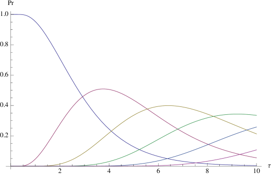
Figure 18: The probabilities of $1,2,\dots,6$ cycles in a uniform random essential CRSF on a large annulus, as a function of the modulus $\tau$.

6.3 The response matrix

Lam and Pylyavskyy [24] studied the response matrices of networks on annuli. Their point of view was to consider the lift $\tilde{\mathcal{G}}$ of the network $\mathcal{G}$ to the universal cover of the annulus. There one can define the response matrix as the limit of response matrices on larger and larger portions of the graph; it is not hard to show that this limit exists. Since the universal cover is planar one can recover some of the results from the planar case like nonnegativity of the non-interlaced minors (non-interlacedness makes sense since the lift $\tilde{\mathcal{G}}$ is planar).

We will take a different approach here which uses the bundle Laplacian for a flat connection. Let $\mathcal{G}$ be a network drawn on an annulus $\Sigma$, with nodes $\mathcal{N}$ which are a subset of the vertices adjacent to the two boundaries of $\Sigma$. Let $\Phi$ be a flat $\mathbb{C}^{*}$-connection with monodromy $z$ around a generator of $\pi_{1}(\Sigma)$. Let $\Delta$ be the associated bundle Laplacian. Let $L$ be the response matrix, defined as before as

$$L=-A+BC^{-1}B^{*}$$

where $\Delta=\begin{pmatrix}A&B\\ B^{*}&C\end{pmatrix}.$ Now entries in $L$ are rational functions of $z$ (with coefficients which depend on the conductances).

What can be said about EIT on annular networks?

For circular planar networks it was very useful to have combinatorial interpretations (in terms of groves) of the entries and minors of the response matrix. We have similar interpretations in the present case. The following theorem of [21] holds for any network with line bundle (not just networks on an annulus). Compare Theorem 4.3 above.

Theorem 6.2 ([21]).

Let $Q,R,S,T$ be a partition of $\mathcal{N}$ and $|R|=|S|$. Then $\det L_{R\cup T}^{S\cup T}$ is the ratio of two terms: the denominator is the weighted sum of CRSFs; the numerator is a signed weighted sum of cycle-rooted groves of $\mathcal{G}_{T}$, the graph $\mathcal{G}$ in which all nodes in $T$ are considered internal, the nodes in $Q$ are in singleton parts, and in which nodes in $R$ are paired with nodes in $S$, with the sign being the sign of the pairing permutation, times the parallel transports from $S$ to $R$:

$$\det L_{R,T}^{S,T}=\sum_{\text{{permutations} $\rho$}}(-1)^{\rho}\frac{\mathcal{Z}\big{[}{}_{r_{1}}^{s_{\rho(1)}}|\cdots|_{r_{k}}^{s_{\rho(k)}}|q_{1}|\cdots|q_{\ell}\big{]}}{\mathcal{Z}[1|2|\cdots|n]}$$

Here the numerator $\mathcal{Z}\big{[}{}_{r_{1}}^{s_{\rho(1)}}|\cdots|_{r_{k}}^{s_{\rho(k)}}|q_{1}|\cdots|q_{\ell}\big{]}$ is the weighted sum of CRG’s in which there are tree components connecting $r_{i}$ to $s_{\rho(i)}$ for each $i$; the weight is the product of the edge conductances, times the product over all cycles $\gamma$ of $2-w(\gamma)-1/w(\gamma)$ (where $w(\gamma)$ is the monodromy of the cycle $\gamma$) and times the product of the parallel transports from the $r_{i}$ to the $s_{\rho(i)}$ along the edges of the trees. We use the notation $\mathcal{Z}$ as opposed to $Z$ to remind us that we are dealing with the bundle Laplacian.

On an annulus with flat connection, it is convenient to have the connection supported on a “zipper”, that is, the set of faces crossing a shortest path in the dual graph from one boundary component to the other, as in Figure 19. In such a case the monodromy along a path from a node to another node is $1,z$ or $z^{-1}$ if the nodes are on the same boundary; it is a power of $z$ if the nodes are on different boundaries, and it is $z^{\pm 1}$ for a topologically nontrivial cycle.

Figure 19: The parallel transport on an annulus can be supported on a zipper.

If particular if $i$ and $j$ are nodes on opposite boundaries then

$$L_{ij}\mathcal{Z}_{\text{unc}}=\sum_{k\in\mathbb{Z}}C_{k}z^{k},$$

where $C_{k}$ is the weighted sum of CRGs with a component tree connecting $i$ to $j$, no cycles (a cycle is precluded by the existence of a path from $i$ to $j$), and where $k$ is the signed number of times the path from $i$ to $j$ crosses the zipper.

Thus $L_{ij}\mathcal{Z}_{\text{unc}}$ is a Laurent polynomial of $z$ with nonnegative coefficients.

Here is another example. Suppose $A=\{a_{1},a_{2}\}$ are nodes on one boundary and $B=\{b_{1},b_{2}\}$ are nodes on the other. Then by the Theorem $L_{A}^{B}\mathcal{Z}_{\text{unc}}$ contains terms in which $a_{1}$ is paired with $b_{1}$ (and $a_{2}$ with $b_{2}$) and, with an opposite sign terms in which $a_{1}$ is paired with $b_{2}$ and $a_{2}$ with $b_{1}$. However these two types of terms differ by an power of $z$. Suppose for example that the zipper is as shown in Figure 19. Then any term ${}_{a_{1}}^{b_{1}}|{}_{a_{2}}^{b_{2}}$ has an even power of $z$ and ${}_{a_{1}}^{b_{2}}|{}_{a_{2}}^{b_{1}}$ has an odd power of $z$. Thus $L_{A}^{B}\mathcal{Z}_{\text{unc}}$ is a Laurent polynomial in $z$ with coefficients of alternating sign.

6.4 Minimality and reconstruction

6.4.1 Minimal networks on the annulus: landscapes

Let $\mathcal{G}$ be a minimal network on an annulus $\Sigma$ with $n_{1}$ nodes on one boundary and $n_{2}$ on the other. As discussed, let $\tilde{\mathcal{G}}$ be the lift of $\mathcal{G}$ to the strip, the universal cover of the annulus. The medial strands come in four types:

1. they connect stubs on the lower boundary of the strip (the rocks);

2. they connect stubs on the upper boundary of the strip (the clouds);

3. they connect stubs across the boundaries (the trees);

4. they form bi-infinite paths along the strip (the river).

We can perform Y-Delta transformations so that the strands of the first, second and fourth type do not intersect (that is, no strand of the first type intersects a strand of the second or fourth type, although it may intersect other strands of the first type, etc.) As long as there is at least one tree strand, then we can “untwist” the river strands so that they are all parallel and noncrossing.

The picture is then like a landscape; the rocks at the bottom, interspersed with trees which grow up to mingle with the clouds, and the river runs through the trees but does not touch the clouds or rocks. See Figure 20 and 21.

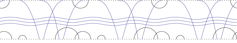
Figure 20: A landscape: the general form of a minimal network on an annulus (we show only the medial graph, and on the universal cover of the annulus).

Figure 21: Bow falls, Banff.

6.4.2 Reconstruction

The reconstruction of the conductances on a minimal annular network as a function of the response matrix is open in general. Lam and Pylyavskyy [24] worked out the reconstruction for the “grid” network of Figure 22, whose medial graph is a grid.

Figure 22: The “grid” network on an annulus.

The new feature of this reconstruction problem is that the solution is not unique. If the medial graph of $\mathcal{G}$ has $k$ topologically nontrivial cycles, then there are generically $k!$ solutions to the reconstruction. The idea is that given a set of conductances on $\mathcal{G}$ one can permute the parallel strands of the medial graph and get another solution. How does one permute two strands? This follows from the discussion of combing in Theorem 5.1 above. See Figure 13. One introduces a pair of edges of opposite conductance $c,-c$; this has no effect on the current flow or response matrix. Now perform Y-Delta moves around the annulus to exchange the adjacent strands. There is a unique choice of $c$ for which the added edge, when it comes back around, will again have conductance $c$; it then can be removed along with the parallel edge of conductance $-c$.

In [24] it is conjectured that reconstruction is possible on all minimal annular networks.

7 Periodic networks and networks on the torus

Let $\mathcal{G}$ be a network on a torus. By this we mean a network $\mathcal{G}$, with no boundary, embedded on a torus in such a way that every complementary component is contractible.

For concreteness we suppose the torus is $\mathbb{T}^{2}=\mathbb{R}^{2}/\mathbb{Z}^{2}$ (but the network can be arbitrary). The lifted network $\tilde{\mathcal{G}}$ on the universal cover $\mathbb{R}^{2}$ of $\mathbb{T}^{2}$ is a periodic planar network.

This case differs from the previous cases of circular planar and annular networks in that the underlying surface has no boundary, so we do not introduce any nodes. Remarkably we can still have a complete theory about reducibility, minimal networks, and the reconstruction problem.

7.1 The spectral curve of $\Delta$

Let $\Phi$ be a flat line bundle on $\mathcal{G}$ with monodromy $z_{1},z_{2}$ around the standard generators of the homotopy group of $\mathbb{T}^{2}$. Let $\Delta=\Delta_{\Phi}$ the associated Laplacian. See for example Figure 23. In this example the associated Laplacian determinant $P(z_{1},z_{2})=\det\Delta$ is (with the vertices in the order indicated)

$$P(z_{1},z_{2})=\det\left(\begin{array}[]{cccc}6&-3-z_{1}^{-1}&-1-z_{1}^{-1}&0\\ -3-z_{1}&6&0&-1-z_{2}^{-1}\\ -1-z_{2}&0&4&-1-z_{1}^{-1}\\ 0&-1-z_{2}&-1-z_{1}&4\end{array}\right)=$$

$$=3z_{1}^{2}+\frac{3}{z_{1}^{2}}-4z_{1}z_{2}-\frac{4z_{1}}{z_{2}}-\frac{4z_{2}}{z_{1}}-\frac{4}{z_{1}z_{2}}-76z_{1}-\frac{76}{z_{1}}+z_{2}^{2}+\frac{1}{z_{2}^{2}}-52z_{2}-\frac{52}{z_{2}}+264.$$ (17)

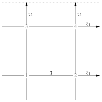
Figure 23: The $2\times 2$ grid on a torus; in this example all edges have conductance $1$ except for the one indicated which has conductance $3$.

In general $P$ is a (Laurent) polynomial with coefficients which are polynomials in the conductances. It is called the characteristic polynomial of $\Delta$. The curve $\{(z_{1},z_{2})\in\mathbb{C}^{2}~{}|~{}P(z_{1},z_{2})=0\}$ is the spectral curve of $\Delta$. Note that $P$ is symmetric: $P(z_{1},z_{2})=P(z_{1}^{-1},z_{2}^{-1})$. This is because we can write $\Delta=d^{*}{\cal C}d$ where $d^{*}$ is the Hermitian transpose of $d$ when $|z_{1}|=|z_{2}|=1$.

The Newton polygon of the network $\mathcal{G}$ on the torus is the Newton polygon of $P$, that is, the convex hull of

$$\{(i,j)\in\mathbb{Z}^{2}~{}|~{}z_{1}^{i_{1}}z_{2}^{j_{2}}\text{ is a coefficient of $P$}\}.$$

It is a centrally symmetric polygon centered at $(0,0)$.

By Theorem 5.2 we can write

$$P(z_{1},z_{2}) = \sum_{\text{CRSFs}}\left(\prod_{e}c_{e}\right)(2-w-1/w)^{k},$$ (18)

$$= \sum_{(r,s)\neq(0,0)}C_{r,s}(2-z_{1}^{i}z_{2}^{j}-z_{1}^{-i}z_{2}^{-j})^{k},$$

where in the first line we used the fact that in a CRSF on a torus all cycles have the same homology class, and in the second line we sum over all homology classes $(r,s)\in\mathbb{Z}^{2}$ (we need only sum over one of each pair $(r,s),(-r,-s)$) where $(r,s)=(ik,jk)$ with $i,j$ being relatively prime. The coefficient $C_{r,s}$ is the weighted sum of CRSFs with $k$ cycles of homology class $(i,j)$, that is (if we orient the cycles in the same direction) of total homology class $(r,s)$.

This shows that the $z_{1}^{r}z_{2}^{s}$ coefficient of $P(z_{1},z_{2})$ is only due to the CRSFs with cycles in direction $r/s$. Thus the Newton polygon $N$ tells us which homology classes of CRSFs are possible for $\mathcal{G}$; equivalently, the maximal number of vertex-disjoint cycles in $\mathcal{G}$ which have homology class $(i,j)$ is determined by the integer point in $N$ which is farthest from the origin in direction $(i,j)$.

In the above example (17), $P$ can be written in “Newton polygon form”

$$P=\begin{matrix}&&1&&\\ &-4&-52&-4&\\ 3&-76&264&-76&3\\ &-4&-52&-4&\\ &&1&&\end{matrix}.$$

From this, one can write $P$ in a unique way in form (18):

$$P(z_{1},z_{2})=3(2-z_{1}-\frac{1}{z_{1}})^{2}+64(2-z_{1}-\frac{1}{z_{1}})+(2-z_{2}-\frac{1}{z_{2}})^{2}+48(2-z_{2}-\frac{1}{z_{2}})+\\ +4(2-z_{1}z_{2}-\frac{1}{z_{1}z_{2}})+4(2-\frac{z_{1}}{z_{2}}-\frac{z_{2}}{z_{1}}).$$ (19)

Thus there are, for example, exactly $48$ CRSFs with a single cycle which has homology class $(0,\pm 1)$.

7.2 UST on the plane

Let us say briefly a few words about the UST on the plane.

Let $\tilde{\mathcal{G}}$ be the periodic planar graph which is the lift of $\mathcal{G}$ to $\mathbb{R}^{2}$. Pemantle [28] showed that there is a UST measure on spanning trees of $\tilde{\mathcal{G}}$ which is the limit of the UST measure on larger and larger tori $\tilde{\mathcal{G}}_{n}\stackrel{{\scriptstyle\text{def}}}{{=}}\tilde{\mathcal{G}}/n\mathbb{Z}^{2}$.

The Free Energy of this measure is the limit

$$F=\lim_{n\to\infty}\frac{1}{n^{2}}\log Z_{n},$$

where $Z_{n}$ is the partition sum for spanning trees on $\tilde{\mathcal{G}}_{n}$.

There is a nice formula for $F$

$$F=\frac{1}{(2\pi i)^{2}}\int_{|z_{1}|=1}\int_{|z_{2}|=1}\log P(z_{1},z_{2})\frac{dz_{1}}{z_{1}}\frac{dz_{2}}{z_{2}}$$

which arises from the exact formula

$$Z_{n}(z_{1},z_{2})=\prod_{\zeta_{1}^{n}=z_{1}}\prod_{\zeta_{2}^{n}=z_{2}}P(\zeta_{1},\zeta_{2})$$

(obtained by Fourier analysis of $\tilde{\mathcal{G}}_{n}$) by taking logs and replacing the Riemann sum with an integral.

One can analyze the limiting UST measure using the fact that edge process is determinantal with kernel $T$ given by the Transfer Current matrix: $T(e,e^{\prime})$ is the current across $e^{\prime}$ when one unit of current enters the graph at $e_{+}$ and exits at $e_{-}$. In terms of the Greens function we can write

$$T(e,e^{\prime})=G(e_{+},e^{\prime}_{+})-G(e_{+},e^{\prime}_{-})-G(e_{-},e^{\prime}_{+})+G(e_{-},e^{\prime}_{-}).$$

The Green’s function $G(v,v^{\prime})$ on $\tilde{\mathcal{G}}$ has a formula involving the Fourier coefficients of $1/P(z_{1},z_{2})$: more precisely, an integral over the unit torus $|z_{1}|=|z_{2}|=1$ of an expression $z_{1}^{x}z_{2}^{y}Q(z_{1},z_{2})/P(z_{1},z_{2})$ where $(x,y)$ is the translation from $v$ to $v^{\prime}$ and $Q$ is a polynomial depending on where $v,v^{\prime}$ sit in their respective fundamental domains. In particular the transfer current has an exact asymptotic expression.

7.3 Medial strands and minimality

Recall that two networks on $\mathbb{T}^{2}$ are topologically equivalent if one can be obtained from the other (disregarding conductances) by electrical transformations. We say that they are electrically equivalent if their characteristic polynomials are the same (compare this definition with the one for networks with boundary in section 5).

Theorem 7.1.

Two networks on a torus are topologically equivalent if and only if their Newton polygons are equal.

Proof.

It is not hard to show that electrical transformations do not change $N$. The simplest reason is because there is a bijection on the CRSFs of the “before” and “after” networks, and the set of CRSFs determines $N$.

So it suffices to show that $N$ determines a minimal network up to electrical equivalence. Suppose $N$ has $2n$ integer boundary points $v_{0},\dots,v_{2n-1}$ in cclw order. Let $e_{i}$ be the edge joining $v_{i}$ to $v_{i+1}$; it is antiparallel with $e_{n+i}$ because $P$ is centrally symmetric. The proof now follows from the following lemma. ∎

Lemma 7.2.

The strands of a minimal network are in bijection with, and have homology classes equal to, the $n$ edge pairs $\{e_{i},e_{i+n}\}$.

Proof.

Since the network is minimal we can isotope the strands on the torus so that they are geodesics for a Euclidean structure. Then we orient the strands so that their $y$ coordinate is increasing, or if they have no $y$ component, the $x$ component is increasing.

Let $S_{1},\dots,S_{k}$ be the strands, and let $e_{i}=(x_{i},y_{i})\in\mathbb{Z}^{2}$ be the homology class of $S_{i}$. The length $2k_{i}$ of $S_{i}$ (that is, the number of edges of the corresponding zig-zag path of $\mathcal{G}$) is then determined by $2k_{i}=\sum_{j}|e_{i}\wedge e_{j}|$ since exactly two strands cross at each edge of $\mathcal{G}$.

Every strand gives a constraint on the homology class of a CRSF: for any CRSF with homology class $\omega$ we must have

$$|\omega\wedge e_{i}|\leq k_{i},$$ (20)

since $|\omega\wedge e_{i}|$ is the intersection number of the CRSF with the strand $S_{i}$.

Suppse the $S_{i}$ are indexed in order of decreasing slope $x_{i}/y_{i}$. Let $N_{S}$ be the convex polygon with side vectors $e_{1},\dots,e_{k},-e_{1},\dots,-e_{k}$ in cclw order. It has vertices $v_{1},v_{2},\dots,v_{k},-v_{1},-v_{2},\dots,-v_{k}$ where

$$v_{i}=\frac{1}{2}(e_{1}+\dots+e_{i-1}-e_{i}-\dots-e_{k}).$$

We claim that $N_{S}$ is the subset of $\omega\in\mathbb{R}^{2}$ which satisfy the constraints (20). To see this, note that if $v_{i},v_{i+1}$ are consecutive vertices of $N_{S}$ and $e_{i}$ is the vector between them, then

$$2v_{i}\wedge e_{i} = e_{1}\wedge e_{i}+\dots+e_{i-1}\wedge e_{i}-e_{i+1}\wedge e_{i}-\dots-e_{k}\wedge e_{i}$$

$$= \sum_{j}|e_{j}\wedge e_{i}|$$

$$\leq 2k_{i}$$

and similarly for $v_{i+1}$. Thus $v_{i},v_{i+1}$ satisfy the maximal possible constraint.

Thus $N\subset N_{S}$. To see that $N=N_{S}$, is suffices to construct a CRSF with homology class equal to each of the vertices $v_{i}$ of $N_{S}$. To construct a set of cycles with homology class $v_{1}=\frac{1}{2}(-e_{1}-e_{2}-\dots-e_{k})$, for example, put weight $-1/2$ on each edge of the zig-zag path of $S_{i}$ (in the orientation defined above). Each edge of $\mathcal{G}$ will then have weight $0$ or $\pm 1$; since we assumed that the strands were drawn geodesically, at each vertex there is exactly one incoming and one outgoing edge. The oriented edges with weight $1$ form a set of vertex disjoint cycles of the homology class $\omega$. ∎

7.4 Harnack curves and characterization of spectral curves

The Laurent polynomial $P=\det\Delta$ has the following properties:

1. $P$ has real coefficients.

2. $P$ is symmetric: $P(z_{1},z_{2})=P(z_{1}^{-1},z_{2}^{-1})$.

3. $P(1,1)=0$.

4. $\{P=0\}$ is a Harnack curve.

What we call Harnack curves were studied by Harnack and called simple Harnack curves by Mikhalkin in [26]. The definition given by Mikhalkin in [26] involves a topological condition on the real locus; in [27] a more concise characterization was given: a curve is Harnack if it intersects each torus $\{|z|=c_{1},|w|=c_{2}\}$ in at most two points (which are necessarily complex conjugates if not real). In particular the map $(z,w)\mapsto(\log|z|,\log|w|)$ which maps the curve into $\mathbb{R}^{2}$ is generically $2$ to $1$. The image of $P=0$ under this map is the amoeba of $P$. See Figure 24 for the amoeba of the example above.

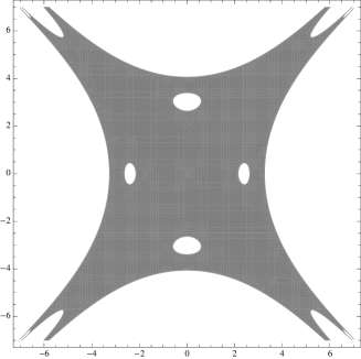
Figure 24: The amoeba (shaded) of the curve of Figure 23 above. The boundary of the amoeba is the real locus of $P=0$; a model of $P=0$ can be obtained by gluing two copies of the shaded region together along their common boundary.

Remarkably, the four properties above characterize the characteristic polynomials of networks on a torus:

Theorem 7.3.

[15, 12] For any polynomial $P$ satisfying the above properties there is a network $\mathcal{G}$ whose characteristic polynomial is $P$. The set of minimal networks with polynomial $P$, modulo electrical transformations, is a real torus of dimension $g/2,$ where $g$ is the geometric genus (the number of real ovals of the amoeba of $P$).

8 Other surfaces

For surfaces other than the annulus and torus, the fundamental group will be nonabelian so it is appropriate to use an $\text{SL}_{2}(\mathbb{C})$-connection on $\mathcal{G}$ rather than a $\mathbb{C}^{*}$-connection.

Although we understand very little about this situation, there is one positive result. Considering the Laplacian determinant as a function on the moduli space of flat $\text{SL}_{2}(\mathbb{C})$-connections, it can be written in a unique way as a sum over CRSFs according to the homotopy types of their cycles. Let us explain this. We define a finite lamination on $\Sigma$ to be an isotopy class of finite pairwise disjoint collection of simple closed curves, none bounding a disk. For example on an annulus there is a finite lamination for each nonnegative integer $k$, $k$ being the number of its cycles.

The cycles in a CRSF form a finite lamination. One can ask the question: for a given finite lamination $\cal L$, what is the weighted sum of CRSFs having cycle set of type ${\cal L}$? We have

Theorem 8.1 ([14, 10]).

$P=\det\Delta$ can be written as

$$P=\sum_{\cal L}C_{\cal L}$$

where the sum is over all finite laminations and $C_{\cal L}$ is the weighted sum (partition sum) of CRSFs of cycle type ${\cal L}$. The coefficients $C_{\cal L}$ are functions of $P$ only, and can be extracted via an appropriate integration of $P$ over the representation variety ${\text{H}om}(\pi_{1}(\Sigma),\text{SL}_{2}(\mathbb{C}))$.

As an example, take $\Sigma$ to be a pair of pants, that is, a sphere minus three disks. Let $\mathcal{G}$ be a network embedded on $\Sigma$. Take a flat $\text{SL}_{2}(\mathbb{C})$-connection on $\mathcal{G}$ with monodromy $A,B,C$ around the three boundary holes, where $ABC=1$.

Then

$$P=\det\Delta=\sum_{i,j,k\geq 0}c_{i,j,k}(2-\mathrm{Tr}A)^{i}(2-\mathrm{Tr}B)^{j}(2-\mathrm{Tr}(AB))^{k}.$$

Given variables $X,Y,Z$ one can choose matrices $A,B$ in $\text{SL}_{2}(\mathbb{C})$ such that $2-\mathrm{Tr}A=X,2-\mathrm{Tr}B=Y,2-\mathrm{Tr}AB=Z$. Then

$$P=P(X,Y,Z)=\sum_{i,j,k\geq 0}c_{i,j,k}X^{i}Y^{j}Z^{k}.$$

One can extract from this expression the coefficients $c_{i,j,k}$.

References

- [1] Aldous, D. The random walk construction of uniform spanning trees and uniform labelled trees. SIAM J. Disc. Math. 3 (1990) 450 - 465.
- [2] Broder, A. (1988). Generating random spanning trees. In: Symp. foundations of computer sci., Institute for Electrical and Electronic Engineers, New York 442 - 447.
- [3] Borchardt, Carl Wilhelm Über eine Interpolationsformel für eine Art Symmetrischer Functionen und über Deren Anwendung. Math. Abh. der Akademie der Wissenschaften zu Berlin (1860) 1 20.
- [4] Burton, Robert; Pemantle, Robin Local characteristics, entropy and limit theorems for spanning trees and domino tilings via transfer-impedances. Ann. Probab. 21 (1993), no. 3, 1329 1371.
- [5] Cayley, Arthur A theorem on trees. Quart. J. Math 23 (1889), 376 378.
- [6] Colin de Verdière, Yves Réseaux électriques planaires. I. Comment. Math. Helv. 69 (1994), no. 3, 351 374
- [7] Colin de Verdière, Yves; Gitler, Isidoro; Vertigan, Dirk, Réseaux électriques planaires. II. (Comment. Math. Helv. 71 (1996), no. 1, 144 167
- [8] Curtis, E. B.; Ingerman, D.; Morrow, J. A. Circular planar graphs and resistor networks. Linear Algebra Appl. 283 (1998), no. 1-3, 115 150
- [9] Dyson, Freeman J. Correlations between eigenvalues of a random matrix. Comm. Math. Phys. 19 1970 235 250.
- [10] Fock, Vladimir; Goncharov, Alexander Moduli spaces of local systems and higher Teichm ller theory. Publ. Math. Inst. Hautes tudes Sci. No. 103 (2006), 1 211.
- [11] Forman, Robin Determinants of Laplacians on graphs. Topology 32 (1993), no. 1, 35 46
- [12] Goncharov, Alexander B.; Kenyon, Richard, Dimers and cluster integrable systems. arxiv:1107.5588
- [13] Kenyon, Richard Dominos and the Gaussian free field. Ann. Probab. 29 (2001), no. 3, 1128 1137.
- [14] Kenyon, Richard Spanning forests and the vector bundle laplacian, arXiv:1001.4028
- [15] Kenyon, Richard; Okounkov, Andrei Planar dimers and Harnack curves. Duke Math. J. 131 (2006), no. 3, 499 524
- [16] Kenyon, Richard; Okounkov, Andrei; Sheffield, Scott Dimers and amoebae. Ann. of Math. (2) 163 (2006), no. 3, 1019 1056
- [17] Kenyon, Richard W.; Propp, James G.; Wilson, David B. Trees and matchings. Electron. J. Combin. 7 (2000), Research Paper 25, 34 pp. (electronic)
- [18] Kenyon, Richard W.; Sheffield, Scott Dimers, tilings and trees. J. Combin. Theory Ser. B 92 (2004), no. 2, 295 317.
- [19] Kenyon, Richard W.; Wilson, David B. Boundary partitions in trees and dimers. Trans. Amer. Math. Soc. 363 (2011), no. 3, 1325 1364
- [20] Kenyon, Richard W.; Wilson, David B. Combinatorics of tripartite boundary connections for trees and dimers. Electron. J. Combin. 16 (2009), no. 1
- [21] Kenyon, Richard W.; Wilson, David B., Positivity in planar networks, in preparation.
- [22] Kirchhoff, G. Über die Auflösung der Gleichungen, auf welche man bei der untersuchung der linearen verteilung galvanischer Ströme geführt wird. Ann. Phys. Chem. 72, 497-508, 1847.
- [23] Lam, Thomas; Pylyavskyy, Pavlo, Electrical networks and Lie theory. arXiv:1103.3475
- [24] Lam, Thomas; Pylyavskyy, Pavlo Inverse problem in cylindrical electrical networks arXiv:1104.4998
- [25] Lawler, Gregory F.; Schramm, Oded; Werner, Wendelin Conformal invariance of planar loop-erased random walks and uniform spanning trees. Ann. Probab. 32 (2004), no. 1B, 939 995.
- [26] Mikhalkin, Grigory, Real algebraic curves, the moment map and amoebas”, Ann. Math. 151 (2000), 309-326.
- [27] Mikhalkin, Grigory; Rullgärd, Hans Amoebas of maximal area. Internat. Math. Res. Notices 2001, no. 9, 441 451.
- [28] Pemantle, Robin Choosing a spanning tree for the integer lattice uniformly. Ann. Probab. 19 (1991), no. 4, 1559 1574.
- [29] Postnikov, Alexander, Total positivity, Grassmannians, and networks, arXiv:math/0609764
- [30] Talaska, Kelli Combinatorial formulas for -coordinates in a totally nonnegative Grassmannian. J. Combin. Theory Ser. A 118 (2011), no. 1, 58 66
- [31] H. N. V. Temperley. In Combinatorics: Proceedings of the British Combinatorial Conference 1973, pages 202 204, 1974. London Mathematical Society Lecture Notes Series 13.
- [32] Wilson, David Bruce Generating random spanning trees more quickly than the cover time. Proceedings of the Twenty-eighth Annual ACM Symposium on the Theory of Computing (Philadelphia, PA, 1996), 296 303, ACM, New York, 1996,