LHC signatures of vector boson emission from brane to bulk

Abstract

In the framework of the RSII-$n$ model with $n$ compact and one infinite extra dimensions, we study the production of $Z$-bosons and photons, which escape into the bulk, in association with a jet in $pp$ collisions at the LHC energies. This would show up as the process $pp\to\mbox{jet}+\not\!\!\!E_{T}$. We calculate the distributions in the jet transverse momentum and rapidity and compare them with the Standard Model background $pp\to\mbox{jet}+\nu\bar{\nu}$. We find that the models with $n\geq 4$ can be probed at the collision energy 14 TeV, while searches at 7 TeV are sensitive to models with $n\geq 6$ only.

1 Introduction

One potentially interesting property of the brane-world scenario with extra dimensions of infinite size is the emission of particles from the brane to the bulk [1, 2, 3]. This is one of the ways in which extra dimensions may open up in experiment [4, 5, 6, 7] and also in astroparticle physics and cosmology [8, 9]. A four-dimensional observer residing on the brane is unable to detect particles escaping to infinity in extra dimensions, so the observable signature is missing energy. This is analogous to the ADD model [10], in which the Kaluza-Klein gravitons are also undetectable, and their emission would also manifest itself as missing energy [11]. This analogy goes further: in the case of infinite extra dimensions, the spectrum of four-dimensional masses of escaping particles is continuous, while the KK graviton spectrum is also nearly continuous in the ADD model.

A particular setup that ensures the gravitational quasi-localization of various bulk fields on the brane is a model with one infinite and several compact extra dimensions, equipped with the AdS metric [12, 13, 14, 15, 16]. This is a mild generalization of the original Randall-Sundrum II model [17]. Interestingly, unlike the RSII geometry, the generalized setup quasi-localizes bulk gauge fields [14, 16]. So, it makes sense to consider the emission of vector particles from the brane to the bulk and employ this setup as a concrete example.

In our previous paper [7] we performed a phenomenological analysis of the vector boson emission to the bulk in $e^{+}e^{-}$ collisions. In that case, the promising process is $e^{+}e^{-}\to\gamma+\not\!\!E_{T}$. In this paper we extend the analysis to $pp$ collisions at the LHC energies and study the process $pp\to\mbox{jet}+\not\!\!\!E_{T}$, where energy is carried away by either photon or $Z$-boson emitted into the bulk. Important constraints on the parameters of the setup come from the analysis of the invisible $Z$-boson decay [6] which is due to the fact that the massive $Z$-boson is quasi-localized, rather then exactly localized on the brane. With these constraints, the prospects of observation of the process we study are not particulary bright for $pp$ collisions at 7 TeV: its cross section is small compared to the Standard Model (SM) background $pp\to\mbox{jet}+\nu\bar{\nu}$ unless the number of compact extra dimensions is large, $n\geq 6$. The situation is better for $pp$-collision energy of 14 TeV. In this case, models with smaller numbers of compact extra dimensions can be probed.

This paper is organized as follows. In Sec. 2 we consider the Standard Model in the background of warped $(4+1+n)$-dimensional mectric. We put $SU(2)_{L}\times U(1)_{Y}$ gauge sector of SM into the bulk, while, for definitness, the SM fermions are supposed to be localized on the brane. In Sec. 3 we consider bulk dynamics of the gauge fields. In Sec. 4 we derive differential rates of the processes $pp\to\mbox{jet}+Z_{bulk}$, $pp\to\mbox{jet}+\gamma_{bulk}$. In Sec. 5 we present our results and compare the rates with the background process $pp\to\mbox{jet}+\nu\bar{\nu}$. We conclude in Sec. 6.

2 $SU(2)_{L}\times U(1)_{Y}$ bulk sector of the Standard Model

Let us consider $AdS_{n+5}$ metric with $n$ extra dimensions compactified on a torus $T^{n}$ and one infinite extra dimension,

$$ds^{2}=a^{2}(z)(\eta_{\mu\nu}dx^{\mu}dx^{\nu}-\delta_{ij}d\theta^{i}d\theta^{j})-dz^{2}=G_{MN}dx^{M}dx^{N},$$ (1)

where $M,N=0,1,2,3,5,...,n+4,n+5$, indices $\mu,\nu$ run from $0$ to $3$, indices $i,j$ run from $5$ to $(n+4)$ and refer to compact extra dimensions, $\theta^{i}\in[0,2\pi R_{i}]$, $R_{i}$ are the radii of the compact exrta dimensions, the coordinate $x^{n+5}\equiv z$ denotes a non-compact spatial dimension. The warp factor is

$$a(z)=e^{-k|z|}.$$

The metric (1) is a solution to the $(n+5)$-dimensional Einstein equations with fine-tuned bulk cosmological constant and brane tension. The parameter $k$ is determined by the $(5+n)$- dimensional Planck mass and bulk cosmological constant; it is the only free parameter of the model. We call this setup RSII-$n$ model.

We consider $(5+n)$-dimensional $SU(2)_{L}\times U(1)_{Y}$ gauge theory with bulk gauge fields $A^{\alpha}_{M}$, $B_{M}$ and scalar doublet $\Phi$ in the background metric (1). We assume for definiteness that fermions $\psi$ are localized on the brane and hence depend only on four-dimensional coordinates $x$. The action of this model is

$$S=\int d^{4}x\,dz\prod^{n}_{i=1}\frac{d\theta_{i}}{2\pi R_{i}}\sqrt{g}\left[-\frac{1}{4}\left(F^{\alpha}_{MN}\right)^{2}-\frac{1}{4}B^{2}_{MN}+\left(D_{M}\Phi\right)^{\dagger}D_{M}\Phi-V(\Phi)+\delta(z)\mathcal{L}_{F}\right],$$ (2)

where $\mathcal{L}_{F}$ is the fermion Lagrangian,

$$\mathcal{L}_{F}=i\bar{q}_{L}\left(\hat{\partial}-i\widetilde{g}_{1}\frac{Y^{q}_{L}}{2}\hat{B}-i\widetilde{g}_{2}\frac{\sigma_{i}}{2}A^{\alpha}\right)q_{L}+i\bar{q}_{R}\left(\hat{\partial}-i\widetilde{g}_{1}\frac{Y^{q}_{R}}{2}\hat{B}\right)q_{R},$$

where we consider light quarks only and neglect their masses; summation over quark flavors is assumed. Here $\widetilde{g}_{2}$ and $\widetilde{g}_{1}$ are the $SU(2)_{L}\times U(1)_{Y}$ bulk couplings, respectively, and $V(\Phi)$ is the standard Higgs potential. We consider the Higgs phase of the theory and perform the usual redefinition of the gauge fields,

$$Z_{M}=\frac{1}{\sqrt{\widetilde{g}^{2}_{1}+\widetilde{g}^{2}_{2}}}\left(-\widetilde{g}_{1}B_{M}+\widetilde{g}_{2}A^{3}_{M}\right),\quad A_{M}=\frac{1}{\sqrt{\widetilde{g}^{2}_{1}+\widetilde{g}^{2}_{2}}}\left(\widetilde{g}_{2}B_{M}+\widetilde{g}_{1}A^{3}_{M}\right),$$

$$W_{M}^{\pm}=\frac{1}{\sqrt{2}}\left(A_{M}^{1}\mp iA_{M}^{2}\right).$$

Then the relevant part of the action (2) takes the following form:

$$S=\int d^{4}x\,dz\prod^{n}_{i=1}\frac{d\theta_{i}}{2\pi R_{i}}\sqrt{g}\Bigl{[}-\frac{1}{4}F^{2}_{MN}-\frac{1}{2}|\,W_{MN}\,|^{2}+m^{2}_{W}|\,W_{M}\,|^{2}-\frac{1}{4}Z^{2}_{MN}+\frac{1}{2}m^{2}_{Z}Z^{2}_{M}+\delta(z)\mathcal{L}_{f}\Bigr{]},$$

where $m_{W}^{2}=\frac{1}{4}\widetilde{g}_{2}^{2}v^{2}$ and $m_{Z}^{2}=\frac{1}{4}(\widetilde{g}_{2}^{2}+\widetilde{g}_{1}^{2})v^{2}$ are the bulk masses squared of the gauge fields. Note that photon remains massless. Here $\mathcal{L}_{f}$ is the quark Lagrangian in the Higgs phase, $\mathcal{L}_{f}=\mathcal{L}_{f,EM}+\mathcal{L}_{f,W}$, where

$$\mathcal{L}_{f,EM}=e_{(5)}\sum_{q}Q_{q}\,\bar{q}\gamma^{\mu}A_{\mu}q,$$

$$\mathcal{L}_{f,W}=\frac{\widetilde{g}_{2}}{2\sqrt{2}}\left(\bar{u}\gamma^{\mu}(1-\gamma^{5})W^{+}_{\mu}d+h.c.\right)+\frac{\widetilde{g}_{2}}{2\cos\theta_{W}}\sum_{q=u,d}\bar{q}\gamma^{\mu}\left(T^{3}_{q}(1-\gamma^{5})-2Q_{q}\sin^{2}\theta_{W}\right)Z_{\mu}q,$$

where $e_{(5)}=\widetilde{g}_{2}\sin\theta_{W}=\widetilde{g}_{1}\cos\theta_{W}$ is the bulk electromagnetic coupling and $\,Q_{q}$ is the quark electric charge.

3 Bulk dynamics of the gauge fields

3.1 Bulk Z-boson

In this section we study the properties of the bulk vector fields. We assume that the sizes of compact extra dimensions are small, so that at energies of interest we have $\sqrt{s}\ll 1/R_{i}$. Then the masses of KK modes inhomogeneous in compact dimensions are large and we can ignore KK excitations on the torus. Hence, we take into account only the gapless and continuous KK spectrum corresponding to the motion along the $z$ direction. Before proceeding further, let us discuss the properties of the usual $Z$-boson in this model. Since the fermions couple only to the components $Z_{\mu}$ of the field $Z_{M}$, it is consistent to set $Z_{5}=...=Z_{n+5}=0$ and split the $Z$-boson wave function into longitudinal and transverse parts, $Z^{\mu}=p^{\mu}Z_{L}(p,z)+\epsilon^{\mu}Z_{T}(p,z)$. Once the fermion masses are neglected, the fermion currents are conserved on the brane, so the longitudinal $Z$-bosons are not emitted. The equation of motion for the transverse mode $Z_{T}(p,z)$ is

$$\left(-\partial^{2}_{5}+(2+n)k\,\mbox{sign}(z)\partial_{5}+m^{2}_{Z}-\frac{m^{2}}{a^{2}}\right)Z_{m}(z)=0,$$ (3)

where $Z_{T}(m,z)\equiv Z_{m}(z)$ and $m$ is the four-dimensional mass. We also note that odd eigenmodes of (3) do not interact with the fermions localized on the brane. Even eigenmodes $Z_{m}(z)$ are normalized with the measure $e^{-nk|z|}$:

$$\int dz\,e^{-nk|z|}Z_{m}(z)Z_{m^{\prime}}(z)=\delta(m-m^{\prime}).$$ (4)

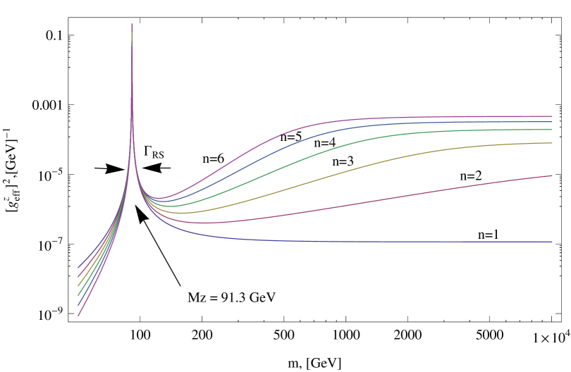
Figure 1:   

Bulk Z-boson coupling parameter squared versus four-dimensional mass $m$ for various numbers of extra dimensions $n$. The values of $k$ for different $n$ are given in Table 3.1.

The solution to Eq. (3) is

$$Z_{m}(z)=\sqrt{\frac{m}{2k}}\,e^{(\frac{n}{2}+1)k|z|}\left[a_{m}J_{\nu}\left(\frac{m}{k}e^{k|z|}\right)+b_{m}N_{\nu}\left(\frac{m}{k}e^{k|z|}\right)\right],$$ (5)

where the order of the Bessel functions is $\nu=\sqrt{\left(1+n/2\right)^{2}+(m_{Z}/k)^{2}}$. The coefficients $a_{m}$ and $b_{m}$ are determined by the boundary condition on the brane $\partial_{z}Z_{m}(+0)-\partial_{z}Z_{m}(-0)=0$ and the normalization condition $a^{2}_{m}+b^{2}_{m}=1$, following from (4). We find

$$a_{m}=-\frac{B_{m}}{\sqrt{B^{2}_{m}+1}},\,\,b_{m}=\frac{1}{\sqrt{B^{2}_{m}+1}},$$

where

$$B_{m}=\frac{N_{\nu-1}(\frac{m}{k})+\frac{k}{m}(\frac{n}{2}+1-\nu)N_{\nu}(\frac{m}{k})}{J_{\nu-1}(\frac{m}{k})+\frac{k}{m}(\frac{n}{2}+1-\nu)J_{\nu}(\frac{m}{k})}.$$ (6)

In the low energy limit only modes with $m\ll k$ are relevant, and the expression (6) simplifies,

$$B_{m}=-\frac{2\,\Gamma^{2}(\frac{n}{2}+1)}{\pi n}\cdot\left(\frac{m}{2k}\right)^{-n}\left(1-\frac{m^{2}_{Z}}{m^{2}}\frac{n}{(n+2)}\right).$$

In this limit, the squared wave function on the brane is

$$Z^{2}_{m}(0)=\frac{\Gamma^{2}(\frac{n}{2}+1)}{\pi^{2}(1+B^{2}_{m})}\cdot\left(\frac{m}{2k}\right)^{-n-1}=\frac{n^{2}}{4}\cdot\frac{m^{4}}{\Gamma^{2}(\frac{n}{2})}\cdot\left(\frac{m}{2k}\right)^{n-1}\frac{1}{(m^{2}-M^{2}_{Z})^{2}+m^{2}\Gamma_{RS}^{2}(m)},$$

where

$$\Gamma_{RS}(m)=\frac{2\pi}{n\Gamma^{2}\left(\frac{n}{2}\right)}m\left(\frac{m}{2k}\right)^{n},\quad M_{Z}=m_{Z}\sqrt{\frac{n}{n+2}}.$$ (7)

Hence, for $k\gg M_{Z}$, $Z$-boson is quasi-localized on the brane, and $M_{Z}$ and $\Gamma_{RS}(M_{Z})$ are its mass and invisible decay width, respectively. In particular, $Z^{2}_{m}(0)$ tends to the delta function as $\Gamma_{RS}\rightarrow 0$:

$$Z^{2}_{m}(0)=\frac{nk}{2}\cdot\frac{1}{\pi}\frac{\Gamma_{RS}}{2}\frac{1}{(m-M_{Z})^{2}+\left(\frac{\Gamma_{RS}}{2}\right)^{2}}\rightarrow\frac{nk}{2}\cdot\delta(m-M_{Z}).$$ (8)

This yields the relation between the four-dimensional and five-dimensional couplings, $e_{(4)}=e_{(5)}\sqrt{\frac{nk}{2}}$.

The fact that $Z$-boson is not exactly localized on the brane implies the lower bounds on the parameter $k$. They come from the requirement that the invisible decay width of $Z$-boson does not exceed the experimental uncertainty [18]:

$$\Gamma_{RS}(M_{Z})\leq\Delta\Gamma^{Z}_{tot}=1.5\,\mbox{MeV}.$$

These bounds are collected in Table 3.1. When presenting numerical results, we will consider the values of $k$ saturating these bounds.

$n$	$1$	$2$	$3$	$4$	$5$	$6$
$k,\mbox{GeV}$	$5.5\cdot 10^{6}$	$2\cdot 10^{4}$	$2.5\cdot 10^{3}$	$900$	$400$	$300$

Table  3.1:    The lower bounds on the parameter $k$ for various numbers of compact extra dimensions $n$.

Coming back to the general discussion, we collect (5) and (6) and find the expression for the wave function at the brane:

$$Z_{m}(0)=\frac{1}{\pi}\sqrt{\frac{2k}{m}}\frac{1}{\sqrt{\left[N_{\nu-1}(\frac{m}{k})+\frac{k}{m}(\frac{n}{2}+1-\nu)N_{\nu}(\frac{m}{k})\right]^{2}+\left[J_{\nu-1}(\frac{m}{k})+\frac{k}{m}(\frac{n}{2}+1-\nu)J_{\nu}(\frac{m}{k})\right]^{2}}}.$$ (9)

This wave function determines the coupling of fermions to the mode $Z_{m}$. Hence, it is useful to introduce the $Z$-boson coupling parameter ${\tt g^{Z}_{eff}}(m)=\sqrt{\frac{2}{nk}}Z_{m}(0)$ . Expanding the Bessel functions at large argument in (9) one finds ${\tt g^{Z}_{eff}}(m)\simeq\sqrt{\frac{2}{\pi nk}}$ for $m/k\gg 1$. We show $[{\tt g^{Z}_{eff}}(m)]^{2}$ as function of $m$ in Fig. 1. Away from the $Z$-pole, the effective coupling increases with $m$ and flattens out at large $m$. Note that the curves in Fig. 1 correspond to different values of $k$. This explains the fact that the large-$m$ asymptotics in Fig. 1 are higher for larger $n$, while for fixed $k$, the asymptotic values of the effective coupling decrease with $n$ as ${\tt g^{Z}_{eff}}\sim n^{-1/2}$.

3.2 Bulk photon

Let us now turn to the bulk photon. We again set $A_{5}=...=A_{n+5}=0$. The equations of motion for the bulk photon are

$$p^{\mu}\partial_{z}A_{\mu}=0,$$ (10)

$$\left(-\partial^{2}_{z}+(2+n)k\,\mbox{sign}(z)\partial_{z}-\frac{p^{2}}{a^{2}}\right)A_{\lambda}+\frac{1}{a^{2}}p^{\mu}p_{\lambda}A_{\mu}=0,$$ (11)

Eqs. (10) and (11) have a constant solution with respect to the $z$-coordinate, $A^{(0)}_{\mu}(p,z)\equiv A^{(0)}_{\mu}(p)=\mbox{const}$. This zero mode describes photon localized on the brane. The normalization condition is

$$\int^{\infty}_{\infty}dz\,e^{-nk|z|}\,|A^{(0)}|^{\,2}=1,$$ (12)

which gives $A^{(0)}=\sqrt{\frac{nk}{2}}$. There is also gapless continuum of bulk modes:

$$A_{m}(z)=\sqrt{\frac{m}{2k}}\,e^{(\frac{n}{2}+1)k|z|}\left[f_{m}J_{\frac{n}{2}+1}\left(\frac{m}{k}e^{k|z|}\right)+g_{m}N_{\frac{n}{2}+1}\left(\frac{m}{k}e^{k|z|}\right)\right],$$ (13)

with the normalization condition $f^{2}_{m}+g^{2}_{m}=1$ and boundary condition on the brane $\partial_{z}A_{m}(+0)-\partial_{z}A_{m}(-0)=0$. Explicitly, Eq. (13) reads:

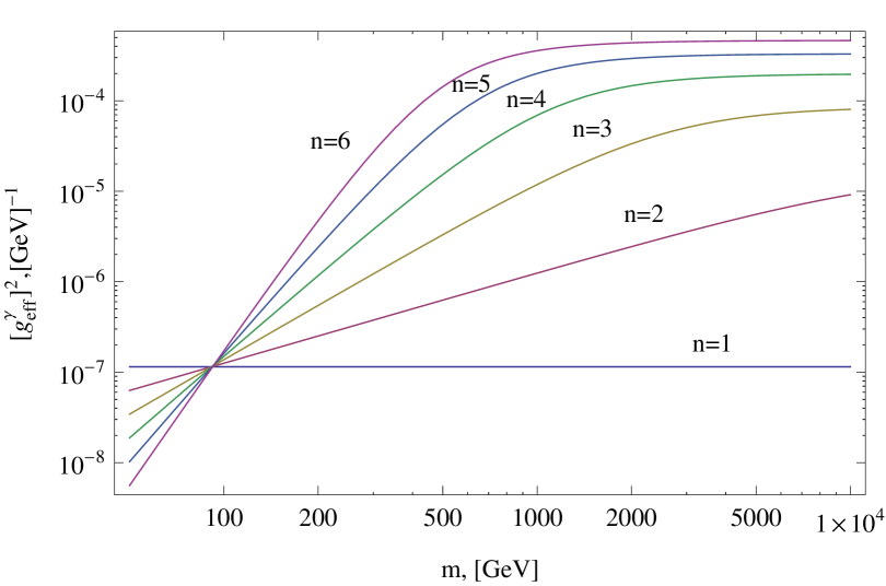
Figure 2:   

Bulk photon coupling squared versus four-dimensional mass $m$ for various numbers of extra dimensions $n$. The values of $k$ for different $n$ are given in Table 3.1.

$$A_{m}(z)=\sqrt{\frac{m}{2k}}\,e^{(\frac{n}{2}+1)k|z|}\frac{\left[N_{\frac{n}{2}}\left(\frac{m}{k}\right)J_{\frac{n}{2}+1}\left(\frac{m}{k}e^{k|z|}\right)-J_{\frac{n}{2}}\left(\frac{m}{k}\right)N_{\frac{n}{2}+1}\left(\frac{m}{k}e^{k|z|}\right)\right]}{\sqrt{J^{2}_{\frac{n}{2}}\left(\frac{m}{k}\right)+N^{2}_{\frac{n}{2}}\left(\frac{m}{k}\right)}},$$ (14)

The interaction of these modes with the brane fermions is determined by their wave functions at the brane, which are given by

$$A_{m}(0)=\frac{1}{\pi}\sqrt{\frac{2k}{m}}\frac{1}{\sqrt{N^{2}_{\nu-1}(\frac{m}{k})+J^{2}_{\nu-1}(\frac{m}{k})}}.$$ (15)

Like in Section 3.1, we introduce the coupling parameter ${\tt g^{\gamma}_{eff}}(m)=\sqrt{\frac{2}{nk}}A_{m}(0)$. For the relatively light modes with $m/k\ll 1$ it is suppressed, ${\tt g^{\gamma}_{eff}}(m)\simeq\sqrt{\frac{n}{2k}}\frac{1}{\Gamma(\frac{n}{2})}\left(\frac{m}{2k}\right)^{\frac{n-1}{2}}$. However, this suppression disappears at high energies, ${\tt g^{\gamma}_{eff}}(m)\simeq\sqrt{\frac{2}{\pi nk}}$ at $m/k\gg 1$. In Fig. 2 we show $[{\tt g^{\gamma}_{eff}}(m)]^{2}$ for various numbers of extra dimensions $n$. We again note that the curves in Fig. 2 correspond to different values of $k$.

Two remarks are in order. First, models with gapless spectra of photons, like the one considered in this paper, are strongly constrained by low energy physics experiment [4, 5] and astrophysics [5, 8]. We are not going to use these constraints in what follows, since they can be evaded by giving a relatively small gap to the bulk vector bosons (see Ref. [19] for concrete example). Second, interactions of the photon zero mode with bulk fields is potentially dangerous [19], since this mode is inhomogeneous in the extra dinmension $z$. Likewise, the interaction of the quasi-localized $Z$-boson with bulk fields is potentially dangerous, so having $SU(2)_{L}$ gauge theory in the bulk may be problematic. We leave this issue for further analysis and proceed with our phenomenological study at the linearized level.

4 The process $pp\to\mbox{jet}+Z_{bulk}(\gamma_{bulk})$

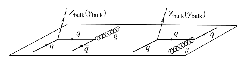
Figure 3:   

The process $pp\to\mbox{jet}++Z_{bulk}(\gamma_{bulk})$.

Within the RSII-$n$ model, the most promising process to search for at $pp$ colliders is $pp\to\mbox{jet}+Z_{bulk}(\gamma_{bulk})$, see Fig. 3, where the jet originates from gluon or quark, and $Z_{bulk}$ and $\gamma_{bulk}$ manifest themselves as missing energy. In this Section we derive the rate of this process. We express it in terms of differential cross section, where the contributions of different KK modes of both bulk $Z$-boson and bulk photon have been summed up. In the RSII-$n$ model this sum is actually the integral over $m$. The differential cross sections for the parton subprocesses $\bar{q}q\to gZ_{bulk}(\gamma_{bulk})$, $g\bar{q}\to\bar{q}Z_{bulk}(\gamma_{bulk})$ and $gq\to qZ_{bulk}(\gamma_{bulk})$ are written as follows:

$$d\sigma^{ij}=(2\pi)^{4}\delta^{(4)}(p_{i}+p_{j}-p_{k}-q)\frac{\overline{\sum}|\mathcal{M}^{ij}|^{2}}{4N_{ij}I}\,\frac{d^{3}p_{k}}{(2\pi)^{3}2p^{0}_{k}}\frac{d^{3}q}{(2\pi)^{3}2q^{0}}\,dm,$$ (16)

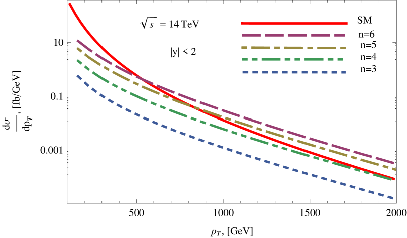
Figure 4:   

Differential cross section of the process $pp\to\mbox{jet}+Z_{bulk}(\gamma_{bulk})$ (dashed lines) versus the jet transverse momentum $p_{T}$ for various numbers of compact extra dimensions $n=3,4,5,6$. The rapidity of a jet is integrated within the interval $|y|<2$. The Standard Model background is $pp\to\mbox{jet}+\nu\bar{\nu}$ (solid line). The center-of-mass energy of incoming protons is $\sqrt{s}=14$TeV. The values of $k$ are given in Table 3.1.

here $I=(p_{i}p_{j})$, the partons are treated as massless, $m$ is the four-dimensional mass of $Z$-boson or photon, whose dispersion relation is $m^{2}=q^{2}$, indices $i,j$ denote the incoming, and $k$ outgoing parton states $(q,\bar{q},g)$. The sum

$$\overline{\sum}=\frac{1}{4}\sum_{pol}\sum_{col}$$

runs over polarization and color. The factor $N_{ij}$ comes from the parton color averaging, it is equal to $N_{\bar{q}q}=N_{c}^{2}$ and $N_{\bar{q}g}=N_{qg}=N_{c}(N_{c}^{2}-1)$. The energies of outgoing parton and bulk particles are equal to $p^{0}_{k}=|{\bf p}_{k}|$ and $q^{0}=\sqrt{m^{2}+{\bf q}^{2}}$, respectively. The four-momenta of incoming partons are $p_{i}=(x_{1}\sqrt{s}/2,0,0,x_{1}\sqrt{s}/2),\quad p_{j}=(x_{2}\sqrt{s}/2,0,0,-x_{2}\sqrt{s}/2),$ where $\sqrt{s}$ is the collider center-of-mass energy. In the following calculation we denote $p_{3}=p_{i3}+p_{j3}$, $p_{T}=\sqrt{p^{2}_{k1}+p^{2}_{k2}}$ and $p_{k3}=p_{T}\sinh y$, where $y$ is the rapidity of the outgoing parton. The energies of the outgoing particles can be rewritten as $p^{0}_{k}=\sqrt{p^{2}_{T}+p_{k3}^{2}}=p_{T}\cosh y$ and $q^{0}=\sqrt{m^{2}+p^{2}_{T}+(p_{3}-p_{T}\sinh y)^{2}}$.

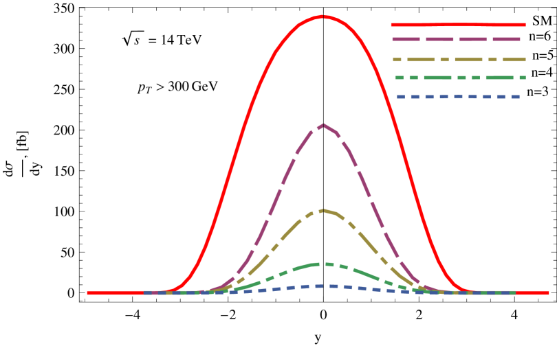
Figure 5:   

Differential cross section of the process $pp\to\mbox{jet}+Z_{bulk}(\gamma_{bulk})$ (dashed lines) versus the jet rapidity $y$ for various numbers of compact extra dimensions $n=3,4,5,6$. The jet transverse momentum is integrated over the range $p_{T}>300$ GeV. The Standard Model background is $pp\to\mbox{jet}+\nu\bar{\nu}$ (solid line). The center-of-mass energy of incoming protons is $\sqrt{s}=14$TeV. The values of $k$ are given in Table 3.1.

The Mandelstam variables are equal to

$$\hat{s}=(p_{i}+p_{j})^{2}=x_{1}x_{2}s,\quad\hat{t}=(p_{i}-p_{k})^{2}=-x_{1}p_{T}\sqrt{s}\,e^{-y},\quad\hat{u}=(p_{j}-p_{k})^{2}=-x_{2}p_{T}\sqrt{s}\,e^{y}.$$

The relation $\hat{s}+\hat{t}+\hat{u}=m^{2}$ gives

$$m^{2}=x_{1}x_{2}s-x_{1}p_{T}\sqrt{s}\,e^{-y}-x_{2}p_{T}\sqrt{s}\,e^{y}=x_{1}x_{2}s\left(1-\frac{1}{2}\frac{x_{T}}{x_{2}}e^{-y}-\frac{1}{2}\frac{x_{T}}{x_{1}}e^{y}\right)\geq 0,$$ (17)

where $x_{T}=2p_{T}/\sqrt{s}$ is the fractional transverse energy of the outgoing parton. The inequality (17) defines the kinematically allowed region for the subprocesses with particles escaping from our brane. The differential cross section of the process $pp\to\mbox{jet}+Z_{bulk}(\gamma_{bulk})$ is written as follows:

$$\frac{d\sigma}{dp_{T}dy}(pp\to\mbox{jet}+Z_{bulk}(\gamma_{bulk}))=\sum_{q=u,d}\int^{1}_{0}dx_{1}\int^{1}_{0}dx_{2}\,\,\theta(m^{2})$$

$$\times\Bigl{\{}\Bigl{[}f_{q}(x_{1},\mu)f_{\bar{q}}(x_{2},\mu)+f_{q}(x_{2},\mu)f_{\bar{q}}(x_{1},\mu)\Bigr{]}\frac{d^{2}\sigma}{dp_{T}dy}(\bar{q}q\to gZ_{bulk}(\gamma_{bulk}))$$

$$+\Bigl{(}\Bigl{[}f_{q}(x_{1},\mu)f_{g}(x_{2},\mu)+f_{\bar{q}}(x_{1},\mu)f_{g}(x_{2},\mu)\Bigr{]}\frac{d^{2}\sigma}{dp_{T}dy}(qg\to qZ_{bulk}(\gamma_{bulk}))$$

$$+\Bigl{[}f_{q}(x_{2},\mu)f_{g}(x_{1},\mu)+f_{\bar{q}}(x_{2})f_{g}(x_{1},\mu)\Bigr{]}\frac{d^{2}\sigma}{dp_{T}dy}(gq\to qZ_{bulk}(\gamma_{bulk}))\Bigr{)}\Bigr{\}}$$ (18)

where $f_{i}(x,\mu)$ are parton distribution functions. The parton differential rates are obtained by integrating Eq. (16) over $m$ and ${\bf q}$:

$$\frac{d\sigma}{dp_{T}\,dy}(ij\to kZ_{bulk}(\gamma_{bulk}))=\frac{p_{T}}{8\pi N_{ij}m\,x_{1}x_{2}s}\overline{\sum}|\mathcal{M}(ij\to kZ_{bulk}(\gamma_{bulk}))|^{2}.$$ (19)

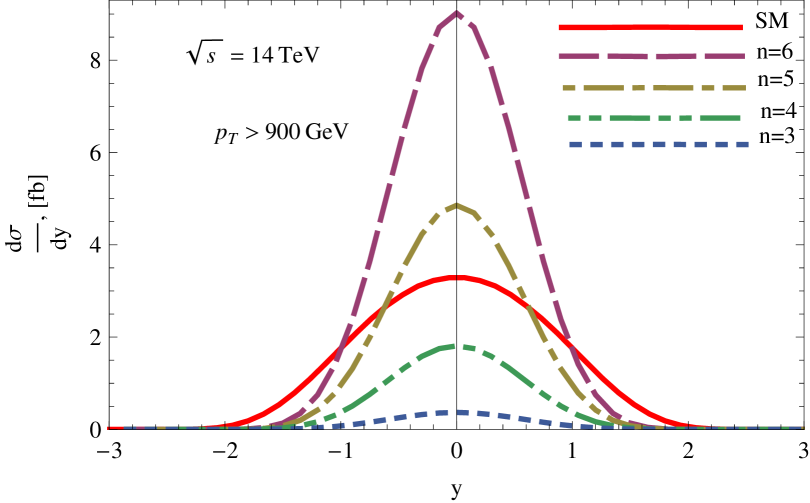
Figure 6:   

Same as in Fig. 5, but with the transverse momentum integrated over the range $p_{T}>900$ GeV.

Squared matrix elements for the subprocesses obey the crossing symmetry relations

$$\overline{\sum}|\mathcal{M}(gq\to qZ_{bulk}(\gamma_{bulk}))|^{2}=-\overline{\sum}|\mathcal{M}(\bar{q}q\to gZ_{bulk}(\gamma_{bulk}))|^{2}\Big{|}_{\hat{s}\leftrightarrow\hat{t}},$$ (20)

$$\overline{\sum}|\mathcal{M}(qg\to qZ_{bulk}(\gamma_{bulk}))|^{2}=-\overline{\sum}|\mathcal{M}(\bar{q}q\to gZ_{bulk}(\gamma_{bulk}))|^{2}\Big{|}_{\hat{s}\leftrightarrow\hat{u}}.$$ (21)

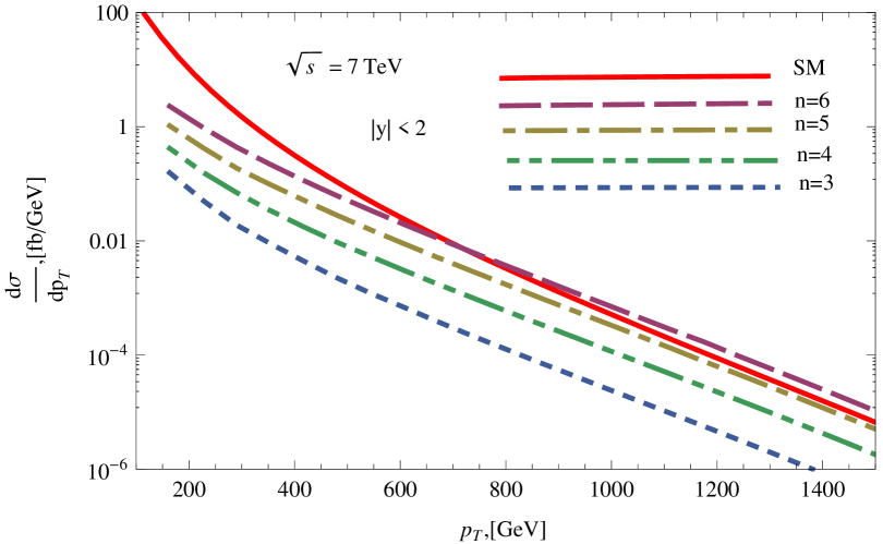
Figure 7:   

Same as in Fig. 4, but for the center-of-mass energy of incoming protons equal to 7 TeV.

Due to the relations (20) and (21), only one squared amplitude for the subprocesses needs to be calculated. For the bulk $Z$-boson in the final state we obtain

$$\overline{\sum}|\mathcal{M}(\bar{q}q\to gZ_{bulk})|^{2}=8\pi^{2}\alpha\alpha_{S}(N^{2}_{c}-1)\sum_{\lambda=L,R}\left(I_{q_{\lambda}}\right)^{2}\frac{\hat{t}^{2}+\hat{u}^{2}+2m^{2}\hat{s}^{2}}{\hat{t}\hat{u}}\cdot\frac{2}{nk}\,Z^{2}_{m}(0),$$ (22)

where $\alpha=e^{2}/(4\pi)$ and $\alpha_{S}=g^{2}_{S}/(4\pi)$ are the electromagnetic and strong couplings, and $Z_{m}(0)$ is the wave function of the bulk $Z$-boson given by Eq. (9). The factor $I^{Z}_{q_{\lambda}}$ is the combination of the weak isospin $T_{q_{\lambda}}^{3}$ and weak hypercharge $Y_{q_{\lambda}}$:

$$I^{Z}_{q_{\lambda}}=T^{3}_{q_{\lambda}}\,\frac{\cos\theta_{W}}{\sin\theta_{W}}-\frac{Y_{q_{\lambda}}}{2}\,\frac{\sin\theta_{W}}{\cos\theta_{W}}.$$

The amplitude similiar to (22) with $\gamma_{bulk}$ in the final state reads

$$\overline{\sum}|\mathcal{M}(\bar{q}q\to g\gamma_{bulk})|^{2}=16\pi^{2}\alpha\alpha_{S}(N^{2}_{c}-1)Q^{2}_{q}\frac{\hat{t}^{2}+\hat{u}^{2}+2m^{2}\hat{s}^{2}}{\hat{t}\hat{u}}\cdot\frac{2}{nk}\,A^{2}_{m}(0),$$ (23)

where $Q_{u}=2/3$, $Q_{d}=-1/3$ are the quark electric charges, and the factor $A_{m}(0)$ is given by Eq. (15).

5 Signal at the LHC

In this section the distributions in jet transverse momentum and jet rapidity are calculated for the process $pp\to\mbox{jet}+\not\!\!E_{T}$, where the energy is carried away from the brane by either bulk $Z$-boson or bulk photon. We compare these distributions with the main Standard Model background that comes from the processes $pp\to\mbox{jet}+\nu\bar{\nu}$. This background has been computed using the program COMPHEP [20]. In our numerical calculations, GRV LO PDFs [21] are used throughout. The factorization scale of the PDFs is fixed at $\mu=1$ TeV. Only $u$ and $d$ flavors are activated since numerical calculations show that the contributions of the other flavors are negligible.

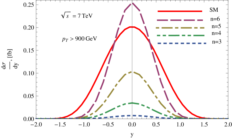
Figure 8:   

Same as in Fig. 6, but for the center-of-mass energy of incoming protons equal to 7 TeV.

We begin our discussion with the case of the proton collision energy equal to 14 TeV. In Fig. 4 we show $p_{T}$ distributions for the processes $pp\to\mbox{jet}+Z_{bulk}(\gamma_{bulk})$ for various numbers of compact extra dimensions $n=3,4,5,6$. The cut on the jet rapidity is $|y|<2$ for both signal and background. For $n=6$ and $n=5$, the signal cross section dominates over the Standard Model for $p_{T}>500$ GeV and $p_{T}>750$ GeV, respectively. The signal is below the background for $n=3,4$. It is clear from Fig. 4 that the cross section of $pp\to\mbox{jet}+Z_{bulk}(\gamma_{bulk})$ grows with the increase of $n$. This is mainly because larger values of $k$ are allowed for larger $n$, see Table 3.1. We pointed out in section 3 ( see also Figs. 1, 2) that the effective coupling of bulk fields has a plateau in the high region. This explains the fact that for any given number of compact dimensions, the ratio of signal to background is higher in the high mode region, and hence at larger $p_{T}$. The jet rapidity distributions with the cut $p_{T}>300$ GeV are shown in Fig. 5. These distributions are correlated with the plots shown in Fig. 4, since the main contribution to the SM background comes from the region $300\mbox{ GeV}<p_{T}<750\mbox{ GeV}$. To enhance the signal with respect to background we consider also the cut $p_{T}>900\mbox{ GeV}$. This is shown in Fig. 6. In the cases $n=5,6$ signal cross sections are larger than the Standard Model background; for $n=4$ the signal is not negligibly small either. These results are in agreement with the $p_{T}$ distributions shown in Fig. 4.

Now we turn to case $\sqrt{s}=7$ TeV. In Fig. 7 we show the jet transverse momentum distribution with the cut $|y|<2$. Obviously, the situation is worse at this energy, and only the case $n\geq 6$ can possibly be probed. This is also clear from Fig. 8, where we plot the jet rapidity distribution with the cut $p>900$ GeV.

6 Summary

In this paper we have performed the study of the production of the bulk $Z$-boson and photon at the LHC in the framework of RSII-$n$ model. This process would show up as $pp\to\mbox{jet}+\not\!\!E_{T}$. The differential distributions in jet rapidity and jet transverse momentum have been calculated and compared with the SM background. Our analys shows that at the total energy $14$ TeV, models with the numbers of compact extra dimensions $n\geq 4$ can be probed, provided that the values of the parameter $k$ of these models is close to the existing lower bounds. The sensivity is much worse at the total collision energy 7 TeV: in that case, one can at best start probing the models with $n\geq 6$.

7 Acknowledgements

We are indebted to E. E. Boos, S. V. Demidov, S. N. Gninenko, D. S. Gorbunov, A. L. Kataev, M. Y. Kuznetsov, D. G. Levkov, A. G. Panin, V. A. Rubakov and M. A. Smolyakov for helpful discussions. This work was supported in part by grants of Russian Ministry of Education and Science NS-5590.2012.2 and GK-16.740.11.0583, grants of the President of Russian Federation MK-2757.2012.2 and MK-1632.2011.2.

References

- [1] V. A. Rubakov and M. E. Shaposhnikov, Phys. Lett. B 125, 136 (1983).
- [2] S. L. Dubovsky, V. A. Rubakov and P. G. Tinyakov, Phys. Rev. D 62, 105011 (2000) [arXiv:hep-th/0006046].
- [3] R. Gregory, V. A. Rubakov and S. M. Sibiryakov, Class. Quant. Grav. 17, 4437 (2000) [arXiv:hep-th/0003109]; S. B. Giddings and E. Katz, J. Math. Phys. 42, 3082 (2001) [arXiv:hep-th/0009176]; C. Ringeval, P. Peter and J. -P. Uzan, Phys. Rev. D 65, 044016 (2002) [hep-th/0109194]; S. L. Dubovsky, V. A. Rubakov and S. M. Sibiryakov, JHEP 0201, 037 (2002) [arXiv:hep-th/0201025]; D. Langlois and M. Sasaki, Phys. Rev. D 68, 064012 (2003) [hep-th/0302069]; R. Koley and S. Kar, Class. Quant. Grav. 22, 753 (2005) [hep-th/0407158]; M. Shaposhnikov, P. Tinyakov and K. Zuleta, Phys. Rev. D 70, 104019 (2004) [hep-th/0411031]; K. Koyama, A. Mennim and D. Wands, Phys. Rev. D 72, 064001 (2005) [hep-th/0504201]; M. Maziashvili, Phys. Lett. B 627, 197 (2005) [hep-ph/0507103]; M. Maziashvili, Phys. Lett. B 635, 36 (2006) [hep-ph/0512362]; A. Melfo, N. Pantoja and J. D. Tempo, Phys. Rev. D 73, 044033 (2006) [arXiv:hep-th/0601161]; S. Khlebnikov, Phys. Rev. D 75, 065021 (2007) [arXiv:hep-ph/0701043]; R. Davies and D. P. George, Phys. Rev. D 76, 104010 (2007) [arXiv:0705.1391 [hep-ph]]; A. Friedland, M. Giannotti and M. L. Graesser, JHEP 0909, 033 (2009) [arXiv:0905.2607 [hep-th]].
- [4] S. N. Gninenko, N. V. Krasnikov and A. Rubbia, Phys. Rev. D 67, 075012 (2003) [hep-ph/0302205].
- [5] A. Friedland and M. Giannotti, arXiv:0709.2164 [hep-ph].
- [6] S. N. Gninenko, N. V. Krasnikov and V. A. Matveev, Phys. Rev. D 78, 097701 (2008) [arXiv:0811.0974 [hep-ph]].
- [7] D. I. Astakhov and D. V. Kirpichnikov, Phys. Rev. D 83, 104031 (2011) [arxiv:hep-ph/1012.1029]
- [8] A. Friedland and M. Giannotti, Phys. Rev. Lett. 100, 031602 (2008).
- [9] H. J. Mosquera Cuesta, A. Penna-Firme and A. Perez-Lorenzana, Phys. Rev. D 67, 087702 (2003) [hep-ph/0203010]; K. Ichiki, P. M. Garnavich, T. Kajino, G. J. Mathews and M. Yahiro, Phys. Rev. D 68, 083518 (2003) [astro-ph/0210052]; T. Tanaka and Y. Himemoto, Phys. Rev. D 67, 104007 (2003) [gr-qc/0301010]; K. Enqvist, A. Mazumdar and A. Perez-Lorenzana, Phys. Rev. D 70, 103508 (2004) [hep-th/0403044]; H. A. Morales-Tecotl, O. Pedraza and L. O. Pimentel, Gen. Rel. Grav. 39, 1185 (2007) [physics/0611241].
- [10] N. Arkani-Hamed, S. Dimopoulus and G. Dvali, Phys. Lett. B 429, 263 (1998) [arXiv:hep-ph/9803315].
- [11] G. F. Giudice, R. Rattazzi and J. D. Wells, Nucl. Phys. B 544, 3 (1999) [arXiv:hep-ph/9811291].
- [12] R. Gregory, Phys. Rev. Lett. 84, 2564 (2000), [arXiv:hep-th/9911015].
- [13] T. Gherghetta and M. E. Shaposhnikov, Phys. Rev. Lett. 85, 240 (2000) [arXiv:hep-th/0004014].
- [14] I. Oda, Phys. Lett. B 496, 113 (2000) [arXiv:hep-th/0006203].
- [15] S. L. Dubovsky, V. A. Rubakov and P. G. Tinyakov, JHEP 0008, 041 (2000) [arXiv:hep-ph/0007179].
- [16] S. L. Dubovsky and V. A. Rubakov, [arXiv:hep-th/0204205].
- [17] L. Randall and R. Sundrum, Phys. Rev. Lett. 83, 4690 (1999) [arXiv:hep-th/9906064].
- [18] C. Amsler et al. [Particle Data Group] Phys. Lett. 667, 1 (2008).
- [19] M. N. Smolyakov, Phys. Rev. D 85, 045036 (2012) [arXiv:1111.1366 [hep-th]].
- [20] E. Boos, V. Bunichev, M. Dubinin, L. Dudko, V. Edneral, V. Ilyin, A. Kryukov and V. Savrin et al., PoS ACAT 08, 008 (2008) [arXiv:0901.4757 [hep-ph]].
- [21] M. Gluck, E. Reya and A. Vogt, Eur. Phys. J. C 5, 461 (1998) [arXiv:hep-ph/9806404].