Strange Quark PDFs and Implications for Drell-Yan Boson Production at the LHC

Abstract

Global analyses of Parton Distribution Functions (PDFs) have provided incisive constraints on the up and down quark components of the proton, but constraining the other flavor degrees of freedom is more challenging. Higher-order theory predictions and new data sets have contributed to recent improvements. Despite these efforts, the strange quark PDF has a sizable uncertainty, particularly in the small $x$ region. We examine the constraints from experiment and theory, and investigate the impact of this uncertainty on LHC observables. In particular, we study $W/Z$ production to see how the $s$-quark uncertainty propagates to these observables, and examine the extent to which precise measurements at the LHC can provide additional information on the proton flavor structure.

I Introduction

I.1 Motivation

Parton distribution functions (PDFs) provide the essential link between the theoretically calculated partonic cross-sections, and the experimentally measured physical cross-sections involving hadrons and mesons. This link is crucial if we are to make incisive tests of the standard model, and search for subtle deviations which might signal new physics.

Recent measurements of charm production in neutrino deeply-inelastic scattering (DIS), visible as di-muon final states, provide important new information on the strange quark distribution, $s(x)$, of the nucleon Abramowicz et al. (1982, 1983, 1984); Berge et al. (1987); Aivazis et al. (1994); Bazarko et al. (1995); Gluck et al. (1996); Alton et al. (2001); Goncharov et al. (2001); Kretzer et al. (2004); Nadolsky et al. (2003); Pumplin et al. (2002); Spentzouris (2002); Tung et al. (2002); Tzanov et al. (2005, 2006). We show that despite these recent advances in both the precision data and theoretical predictions, the relative uncertainty on the heavier flavors remains large. We will focus on the strange quark and show the impact of these uncertainties on selected LHC processes.

The production of $W/Z$ bosons is one of the “benchmark” processes used to calibrate our searches for the Higgs boson and other “new physics” signals. We will examine how the uncertainty of the strange quark PDF influences these measurements, and assess how these uncertainties might be reduced.

I.2 Outline

The outline of the presentation is as follows. In Section 2, we examine the experimental signatures that constrain the strange quark parton distribution. In Section 3 we consider the impact of $s$-quark PDF uncertainties on $W/Z$ production at the LHC, and in Section 4 we summarize our results. Additional details on PDF fits to di-muon data at next-to-leading order are provided in the Appendix.

II Constraining the PDF flavor components

II.1 Extracting the Strange Quark PDF

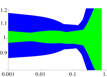
Figure 1: Relative uncertainty of the strange quark PDF as a function of $x$ for $Q=2$ GeV. The inner band is for the CTEQ6.1 PDF set, and the outer band is for the CTEQ6.6 PDF set. The band is computed as the envelope of $s_{i}(x)/s_{0}(x)$ where $s_{0}(x)$ is the central PDF for each set; for CTEQ6.1, $i=[1,40]$, and for CTEQ6.6, $i=[1,44]$.

In previous global analyses, the predominant information on the strange quark PDF $s(x)$ came from the difference of (large) inclusive cross sections for neutral and charged current DIS. For example, at leading-order (LO) in the parton model one finds that the difference between the Neutral Current (NC) and Charged Current (CC) DIS $F_{2}$ structure function is proportional to the strange PDF. Specifically if we neglect the charm PDF and isospin-violating terms, we have Adams et al. (2010)

$$\Delta F_{2}=\frac{5}{18}F_{2}^{CC}-F_{2}^{NC}\sim\frac{x}{6}[s(x)+\bar{s}(x)]\quad.$$ (1)

Because the strange distributions are small compared to the large up and down PDFs, the $s(x)$ extracted from this measurement has large uncertainties. Lacking better information, it was commonly assumed the distribution was of the form

$$s(x)=\bar{s}(x)\sim\kappa[\bar{u}(x)+\bar{d}(x)]/2$$ (2)

with $\kappa\sim\nicefrac{{1}}{{2}}$.

This approach was used, for example, in the CTEQ6.1 PDFs Stump et al. (2003). In Figure 1 we show the relative uncertainty band of the strange quark PDF for the 40 CTEQ6.1 PDF error sets relative to the central value. We observe that over much of the $x$-range the relative uncertainty on the strange PDF is $\,\raisebox{-1.72218pt}{$\stackrel{{\scriptstyle<}}{{\scriptstyle\sim}}$}\,5\%$. The relation of Eq. (2) tells us that this uncertainty band in fact reflects the uncertainty on the up and down sea which is well constrained by DIS measurements; this does not reflect the true uncertainty of $s(x)$.

Beginning with CTEQ6.6 PDFs Nadolsky et al. (2008) the neutrino–nucleon dimuon data was included in the global fits to more directly constrain the strange quark; thus, Eq. (2) was not used, and two additional fitting parameters were introduced to allow the strange quark to vary independently of the up and down sea. We also display the relative uncertainty band for the CTEQ6.6 PDF set in Fig. 1. We now observe that the relative error on the strange quark is much larger than for the CTEQ6.1 set, particularly for $x<0.01$ where the neutrino–nucleon dimuon data do not provide any constraints. We expect this is a more accurate representation of the true uncertainty.

This general behavior is also exhibited in other global PDF sets with errors Martin et al. (2009); Ball et al. (2010); Alekhin et al. (2010); Jimenez-Delgado and Reya (2009). For example, the NNPDF collaboration uses a parameterization-free method for extracting the PDFs; they observe a large increase in the $s(x)$ uncertainty in the small $x$ region which is beyond the constraints of the $\nu$-DIS experiments. (Cf. in particular Fig. 13 of Ref Ball et al. (2010).)

Thus, there is general agreement that the strange quark PDF is poorly constrained, particularly in the small $x$ region.

II.2 Constraints from CCFR and NuTeV

The primary source of information on the strange quark at present comes from high-statistics neutrino–nucleon DIS measurements; in particular, the CCFR and NuTeV dimuon experiments have been used to determine the strange quark PDF with improved accuracy Mason et al. (2007); Tzanov et al. (2006); Zeller et al. (2002); Goncharov et al. (2001); Yang et al. (2001); Alton et al. (2001); Bazarko et al. (1995). Neutrino induced dimuon production ($\nu N\rightarrow\mu^{+}\mu^{-}X$) proceeds primarily through the Cabibbo favored $s\to c$ or $\bar{s}\to\bar{c}$ subprocess. Hence, this provides information on $s$ and $\bar{s}$ directly; this is in contrast to $\Delta F_{2}$ of Eq. (1). CCFR has 5030 $\nu$ and 1060 $\bar{\nu}$ di-muon events, and NuTeV has 5012 $\nu$ and 1458 $\bar{\nu}$ di-muon events, and these cover the approximate range $x\sim[0.01,0.4]$. Additionally, NuTeV used a sign-selected beam to separate the $\nu$ and $\bar{\nu}$ events in order to separately extract $s(x)$ and $\overline{s}(x)$.

II.2.1 Constraints on $s+\bar{s}$

$\chi^{2}/DoF$	CTEQ6M	Free
CCFR $\nu$ dimuon	1.02	0.72
CCFR $\bar{\nu}$ dimuon	0.58	0.59
NuTeV $\nu$ dimuon	1.81	1.44
NuTeV $\bar{\nu}$ dimuon	1.48	1.13
BCDMS $F_{2}^{p}$	1.11	1.11
BCDMS $F_{2}^{d}$	1.10	1.11
H1 96/97	0.94	0.94
H1 98/99	1.02	1.03
ZEUS 96/97	1.14	1.15
NMC $F_{2}^{p}$	1.52	1.49
NMC $F_{2}^{d}/F_{2}^{p}$	0.91	0.91
CCFR $F_{2}$	1.70	1.88
CCFR $F_{3}$	0.42	0.42
E605	0.82	0.83
NA51	0.62	0.52
CDF $\ell$ Asym	0.82	0.82
E866	0.39	0.38
D0 Jets	0.71	0.67
CDF Jets	1.48	1.47
TOTAL $\chi^{2}$	2173	2133

Table 1: We display the $\chi^{2}/DoF$ for selected data sets using the CTEQ6M PDF set Pumplin et al. (2002), and a variant of this (labeled “Free”) which allows for a modified strange quark PDF to accommodate the neutrino dimuon data.

In Table 1 we illustrate how the bulk of the data used in the global fits are relatively insensitive to the strange quark distribution. The first column (labeled “CTEQ6M”) lists the $\chi^{2}/DoF$ for a variety of data sets used in the CTEQ6M fit Pumplin et al. (2002). We have also shown the CCFR and NuTeV dimuon data sets in the table, but these were not used in the CTEQ6M fit. The second column (labeled “Free”) lists results of refitting all the data – including the dimuon data – with a flexible strange quark PDF instead of imposing the relation of Eq. (2); this allows the strange quark PDF to accommodate the dimuon data. Comparing the two columns, we observe that the change of the strange PDF allowed for a greatly improved fit of the dimuon data, while the other data sets are virtually insensitive to this change.

This exercise demonstrates that most of the data sets of the global analysis are insensitive to the details of the strange quark PDF.

II.2.2 Constraints on $s-\bar{s}$

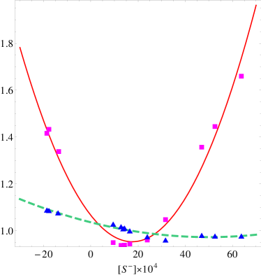
Figure 2: We plot $\chi^{2}/\chi_{0}^{2}$ for the dimuon and the “Inclusive-I” data sets evaluated as a function of the strange asymmetry $[S^{-}]\times 10^{4}$. The fits are denoted with for the dimuons and for “Inclusive-I”. Quadratic approximations to the fits are displayed by the solid (red) line for the dimuons and the dashed (green) line for “Inclusive-I”.

The dimuon data can also provide information on the $s(x)$ and $\bar{s}(x)$ quark PDFs separately. In Fig. 2 we display the relative $\chi^{2}$ for the dimuon and “Inclusive-I” data sets as a function of the strange asymmetry $\left[S^{-}\right]$, where

$$[S^{-}]\equiv\int_{0}^{1}x[s(x)-\bar{s}(x)]\,dx\;.$$ (3)

The “Inclusive-I” data sets (cf., Ref. Olness et al. (2005)) contain the data that is sensitive to $\left[S^{-}\right]$; specifically, the data sets are a) the neutrino $xF_{3}$ data from CCFR and CDHSW as this is proportional to the difference of quark and anti-quark PDFs, and b) the CDF $W$–asymmetry measurement which can receive contributions from the $sg\to Wc$ subprocess. Figure 2 clearly shows that the dimuon data provides the strongest constraints on the strange asymmetry $\left[S^{-}\right]$.

II.3 HERMES

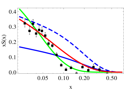
Figure 3: The strange parton distribution $xS(x)=x[s(x)+\bar{s}(x)]$ from the measured Hermes multiplicity for charged kaons evolved to $Q^{2}=2.5\,$GeV². The solid green curve is a Hermes 3-parameter fit: $S(x)=x^{-0.924}e^{-x/0.0404}(1-x)$, the dashed blue curve is the sum of light anti-quarks $x(\bar{u}+\bar{d})$ from CTEQ6L, the blue solid curve is $xS(x)$ from CTEQ6L, and the red solid curve is the $xS(x)$ from CTEQ6.6. Hermes data points and fit are from Ref. Airapetian et al. (2008).

The HERMES experiment measured the strange PDF via charged kaon production in positron–deuteron DIS Airapetian et al. (2008), these results are displayed in Fig. 3. For comparison, the strange quark and total sea distributions from CTEQ6L are also plotted.

The HERMES data suggests that the $x$-dependence of the strange quark distribution is quite different from the form assumed for the CTEQ6 set. In particular, they obtain a strange quark distribution that is suppressed in the region $x\gtrsim 0.1$ but then grows quickly for $x<0.1$ and exceeds the CTEQ6L value in the small $x$ region by more than a factor of two.

To gauge the compatibility of this result with the displayed PDFs, we can replace the initial $s(x)$ distribution with the form preferred by HERMES, and then evaluate the shift of the $\chi^{2}$ with this additional constraint. A preliminary investigation with this procedure indicates that the HERMES $s(x)$ distribution could strongly influence two data sets of the global fits. The first set is the neutrino-nucleon dimuon data which controls $s(x)$ in the intermediate $x$ region. The second set is the HERA measurement of $F_{2}$ in the small $x$ region where the statistical errors are particularly small.

In Fig. 3 we also show $xS(x)$ from CTEQ6.6; while the HERMES data are below the CTEQ6.6 result in the $x\sim 0.1$ region, they agree quite well at both the higher and lower $x$ values.

While these comparisons are sufficient to gauge the general influence of the Hermes result, a complete analysis that includes the Hermes data dynamically in the global fit is required to draw quantitative conclusions.

II.4 CHORUS

The CHORUS experiment Onengut et al. (2004, 2006); Kayis-Topaksu et al. (2008) measured the neutrino structure functions $F_{2}$, $xF_{3}$, $R$ in collisions of sign selected neutrinos and anti-neutrinos with a lead target (lead–scintillator CHORUS calorimeter) in the CERN SPS neutrino beamline. They collected over 3M $\nu_{\mu}$ and 1M $\bar{\nu}_{\mu}$ charged current events in the kinematic range $0.01<x<0.7$, $0.05<y<0.95$, $10<E_{\nu}<100$.

This data was analyzed in the context of a global fit in Ref. Owens et al. (2007) which was based on the CTEQ6.1 PDFs. This analysis made use of the correlated systematic errors and found that the CHORUS data is generally compatible with the other data sets, including the NuTeV data. Thus, the CHORUS data is consistent with the strange distribution extracted in CTEQ6.1.

II.5 NOMAD

The NOMAD experiment measured neutrino-induced charm dimuon production to directly probe the $s$-quark PDF Astier et al. (2000); Petti (2006); Wu et al. (2008). Protons from the CERN SPS synchrotron (450 GeV) struck a beryllium target to produce a neutrino beam with a mean energy of 27 GeV. NOMAD used an iron-scintillator hadronic calorimeter to collect a very high statistics (15K) neutrino-induced charm dimuon sample Petti (2006).

Using kinematic cuts of $E_{\mu 1},E_{\mu 2}>4.5\,$GeV, $15<E_{\nu}<300\,$GeV, and $Q^{2}>1$ GeV² NOMAD performed a leading-order QCD analysis of 2714 neutrino- and 115 anti-neutrino–induced opposite sign dimuon events Astier et al. (2000). The ratio of the strange to non-strange sea in the nucleon was measured to be $\kappa=0.48_{-0.07-0.12}^{+0.09+0.17}$; this is consistent with the values used in the global fits, c.f., Fig. 4.

The data analysis is continuing, and it will be very interesting to include this data set into the global fits as the large dimuon statistics have the potential to strongly influence the extracted PDFs.

II.6 MINER$\nu$A

The cross sections in neutrino DIS experiments from NuTeV, CCFR, CHORUS and NOMAD have been measured using heavy nuclear targets. In order to use these measurements in a global analysis of proton PDFs, these data must be converted to the corresponding proton or isoscalar results de Florian and Sassot (2004); Hirai et al. (2007); Eskola et al. (2009); Schienbein et al. (2008, 2009); Kovarik et al. (2011a, b). For example, the nuclear correction factors used in the CTEQ6 global analysis were extracted from $\ell^{\pm}N$ DIS processes on a variety of nuclei, and then applied to $\nu N$ DIS on heavy nuclear targets. In a series of recent studies it was found that the $\ell^{\pm}N$ nuclear correction factors could differ substantially from the optimal $\nu N$ nuclear correction factors Schienbein et al. (2009); Kovarik et al. (2011a, c, b); Schienbein et al. (2008).

Furthermore, the nuclear corrections depend to a certain degree on the specific observable as they contain different combinations of the partons; the nuclear correction factors for dimuon production will not be exactly the same as the ones for the structure function $F_{2}$ or $F_{3}$. The impact of varying the nuclear corrections on the strange quark PDF has to be done in the context of a global analysis which we leave for a future study.

The MINER$\nu$A experiment has the opportunity to help resolve some of these important questions as it can measure the neutrino DIS cross sections on a variety of light and heavy targets. It uses the NuMI beamline at Fermilab to measure low energy neutrino interactions to study neutrino oscillations and also the strong dynamics of the neutrino–nucleon interactions. MINER$\nu$A completed construction in 2010, and they have begun data collection. MINER$\nu$A can measure neutrino interactions on a variety of targets including plastic, helium, carbon, water, iron, and lead. For $4*10^{20}$ Protons on Target (POT) they can generate over 1M charged current events on plastic.

These high statistics data on a variety of nuclear targets could allow us to accurately characterize the nuclear correction factors as a function of the nuclear $A$ from helium to lead. This data will be very useful in resolving questions about the nuclear corrections, and we look forward to the results in the near future.

II.7 CDF & DO

At the Tevatron, the CDF Aaltonen et al. (2008) and D0 Abazov et al. (2008) collaborations measured $Wc$ final states in $p\bar{p}$ at $\sqrt{S}=1.96$ TeV using the semileptonic decay of the charm and the correlation between the charge of the $W$ and the charm decay. Additionally, a recent study has investigated the impact of the $W$+dijet cross section on the strange PDF Kawamura et al. (2011). These measurement are especially valuable for two reasons. First, there are no nuclear correction factors as the initial state is $p$ or $\bar{p}$. Second, this is in a very different kinematic region as compared to the fixed-target neutrino experiments. Thus, these have the potential to constrain the strange quark PDF in a manner complementary to the $\nu N$ DIS measurements; however, the hadron-hadron initial state is challenging. Using approximately $1\,fb^{-1}$ of data, both CDF and D0 find their measurements to be in agreement with theoretical expectations of the Standard Model. Updated analyses with larger data sets are in progress and it will be interesting to see the impact of these improved constraints on the strange quark PDF.

II.8 Strange Quark Uncertainty

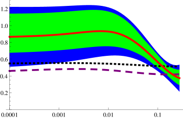
Figure 4: $\kappa(x,Q)$ vs. $x$ for $Q=1.5$ GeV for a selection of PDFs, where $\kappa(x,Q)$ is defined in Eq. (4). The curves (top to bottom) are CTEQ6.6 (solid, red), CTEQ6.5 (dotted, black) and CTEQ6.1 (dashed, purple). The wider (blue) band represents the uncertainty for CTEQ6.6 as computed by Eq. (5), the inner (green) band represents uncertainty given by the envelope of $\kappa(x,Q)$ values obtained with the 44 CTEQ6.6 error sets.

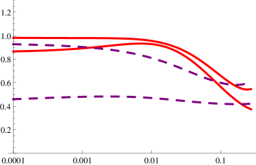
Figure 5: $\kappa(x,Q)$ vs. $x$ showing the evolution from low to high scales. The solid (red) lines are for CTEQ6.6, and the dashed (purple) lines are for CTEQ6.1. The lower pair of lines (red and purple) are for $Q=1.5$ GeV and the upper for $Q=80$ GeV.

The combination of the above results underscores the observation that our knowledge of the strange quark is limited. To illustrate this point in another manner, in Fig. 4 we display $\kappa(x,Q)$ for a selection of PDF sets. Here, we define

$$\kappa(x,Q)=\frac{s(x,Q)}{[\bar{u}(x,Q)+\bar{d}(x,Q)]/2}$$ (4)

which is essentially a differential version of the $\kappa$ parameter of Eq. (2); this allows us to gauge the amount of the strange PDF inside the proton compared to the average up and down sea-quark PDFs. If we had exact $SU(3)$ symmetry we would expect $\bar{u}=\bar{d}=\bar{s}$ and $\kappa(x,Q)\sim 1$. As the strange quark is heavier than the up and down quarks, we expect this component to be suppressed relative to the up and down quarks, and we would predict $\bar{u}\simeq\bar{d}>\bar{s}$ which would yield $\kappa(x,Q)<1$. Thus, $\kappa(x,Q)$ is a measure of the $SU(3)$ breaking across the $x$ and $Q$ range.

In Fig. 4 we observe that the CTEQ6.1 and CTEQ6.5 PDF sets have $\kappa(x,Q)\sim\nicefrac{{1}}{{2}}$; this was by design as the constraint of Eq. (2) was used to set the initial $s(x)$ distribution. The exception is CTEQ6.6 which did not impose Eq. (2); we observe that this set has $\kappa(x,Q)\sim\nicefrac{{1}}{{2}}$ for $x\sim 0.1$ (where the dimuon DIS data has smaller uncertainties), but is a factor of two larger than the other PDF sets for small $x$ values. In Fig. 4 we also show the uncertainty on $s(x)$ computed as Pumplin et al. (2002)

$$\Delta X=\frac{1}{2}\sqrt{\sum_{i=1}^{N_{p}}\left[X(S_{i}^{+})-X(S_{i}^{-})\right]^{2}}$$ (5)

which is shown as a (blue) band; this results in a band which is larger than simply taking the spread of the 44 CTEQ6.6 error PDFs (green band).

In order to show the effect of the DGLAP evolution on the strange distribution, we display $\kappa(x,Q)$ for CTEQ6.1 and CTEQ6.6 at both a low and high $Q$ scale in Fig. 5. As we explore higher scales, the production of $s(x)$ by gluon splitting moves $\kappa(x,Q)$ toward the $SU(3)$-symmetric limit. This trend is especially pronounced at low $x$-values. Thus, as the LHC $W/Z$ production is centered in the range $x\sim 0.01$, we will be particularly interested in the $\kappa(x,Q)$ changes in this region.

These results reflect the relevant $x$-range of the constraints on the strange quark PDF, and how they depend on the $Q$-scale. In the next section we will investigate the implications of this uncertainty on the Drell-Yan $W/Z$ boson production at the LHC.

III Implications for Drell-Yan W/Z Production at the LHC

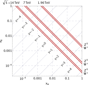
Figure 6: Parton momentum fractions $x_{A}$ and $x_{B}$ accessible in $W$ and $Z$ boson production in the Tevatron Run-2 ($\sqrt{S}=1.96$ TeV), and at the LHC ($\sqrt{S}=\{7,\,14\}$ TeV). The accessible ranges of $x_{A}$ and $x_{B}$ are shown by the solid lines. The contours of the constant rapidity $y$ are shown by the inclined dotted lines.

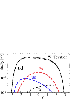
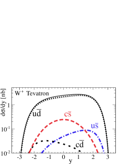
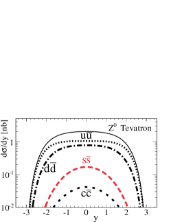
(a) $d\sigma/dy$ for $W^{-}$ (left), $W^{+}$ (middle), $Z^{0}$ (right) boson production at the Tevatron.

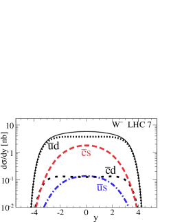
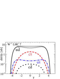
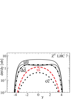
(b) $d\sigma/dy$ for $W^{-}$ (left), $W^{+}$ (middle), $Z^{0}$ (right) boson production at the LHC with $\sqrt{S}=7$ TeV.

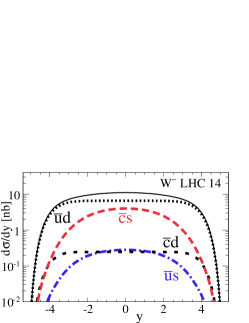
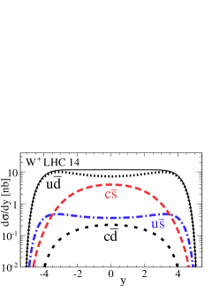
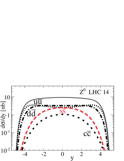
(c) $d\sigma/dy$ for $W^{-}$ (left), $W^{+}$ (middle), $Z^{0}$ (right) boson production at the LHC with $\sqrt{S}=14$ TeV.

Figure 7: Partonic contributions to the differential cross section of on-shell $W^{\pm}/Z$ boson production at LO as a function of the vector boson rapidity. Partonic contributions containing a strange or anti-strange quark are denoted by (red) dashed and (blue) dot-dashed lines. The solid lines show the total contribution.

The Drell-Yan production of $W^{\pm}$ and $Z$ bosons at hadron colliders can provide precise measurements for electroweak observables such as the $W$ boson mass Besson et al. (2008); Krasny et al. (2010) and width, the weak mixing angle in $\gamma^{*}/Z$ production Chatrchyan et al. (2011a), and the lepton asymmetry in $W$ production. These results can measure fundamental parameters of the Standard Model (SM) and constrain the Higgs boson mass. If a Higgs boson is found at the LHC, Drell-Yan $W/Z$ boson production will help in the search for deviations of the SM and to reveal new physics signals Tarrade (2011); Chatrchyan et al. (2011b); Ball et al. (2011a). For instance, new heavy gauge bosons could be discovered in the invariant lepton distribution or new particles and interactions might leave a footprint in the Peskin-Takeuchi $S$ and $T$ parameters Peskin and Takeuchi (1992).

Furthermore, the $W$ and $Z$ boson cross section “benchmark” processes are intended to be used for detector calibration and luminosity monitoring Dittmar et al. (1997); to perform these tasks it is essential that we know the impact of the PDF uncertainties on these measurements. The impact on these benchmark processes, and the Higgs boson production, were studied in Refs. Alekhin et al. (2011); Blumlein et al. (2011); Alekhin et al. (2012). In the following, we will investigate the influence of the PDFs on the rapidity distributions of the Drell-Yan production process. Conversely, it may be possible to use the $W/Z$ production process to further constrain the parton distribution functions in general, and the strange quark PDF in particular. As noted in Ref. Chatrchyan et al. (2011a), when looking for new physics signals it is important not to mix the information used to constrain the PDFs and the new physics as this would lead to circular reasoning.

As we move from the Tevatron to the LHC scattering processes, the kinematics of the incoming partons changes considerably; in Fig. 6 we show the momentum fractions $x_{A}$ and $x_{B}$ of the incoming parton $A$ and parton $B$ for the Tevatron Run-2 ($\sqrt{S}=1.96$ TeV) and the LHC with $\sqrt{S}=7$ TeV and $\sqrt{S}=14$ TeV. The solid (red) lines show the range of $x_{A}$ and $x_{B}$ probed by $W^{\pm}$ and $Z$ boson production. At the Tevatron, values of $x_{A,B}$ down to $2\times 10^{-3}$ are probed for large rapidities of $y_{W/Z}=3$. However, at the LHC much smaller values of $x_{A}$ and $x_{B}$ become important due to the larger CMS energy and broader rapidity span. For $\sqrt{S}=7$ TeV, the PDFs are probed for $x$-values as small as $2\times 10^{-4}$ for rapidities up to $\sim 4.5$. With $\sqrt{S}=14$ TeV, even larger rapidities of $y\sim 5$ and smaller values of $x_{A/B}$ of $4\times 10^{-5}$ might be reached.

III.1 LHC Measurements

The importance of the PDF uncertainties to the LHC measurements was already evident in the 2010 and preliminary 2011 data.

ATLAS presented measurements of the Drell-Yan $W/Z$ production at the $\sqrt{S}=7$ TeV with $35\,pb^{-1}$ Aad et al. (2011). These results include not only the measurement of total cross section and transverse distributions, but also a first measurement of the rapidity distributions for $Z\to l^{+}l^{-}$ as well as $W^{+}\to l^{+}\nu_{l}$ and $W^{-}\to l^{-}\bar{\nu}_{l}$. Additionally, ATLAS has used $W/Z$ production to infer constraints on the strange quark distribution, and they measure $r_{s}=0.5(s+\bar{s})/\bar{d}=1.00_{-0.28}^{+0.25}$ at $Q^{2}=1.9$ GeV² and $x=0.023$ Aad et al. (2012).

CMS has measured the rapidity and transverse momentum distributions for $Z\to l^{+}l^{-}$ production Chatrchyan et al. (2011c) and inclusive $W/Z$ production Chatrchyan et al. (2011d) using $36\,pb^{-1}$ of data. Additionally CMS has measured the weak mixing angle Chatrchyan et al. (2011a), the forward-backward asymmetry in $\gamma^{*}/Z$ production (2011a), and the lepton charge asymmetry in $W$ production (2011b); Chatrchyan et al. (2011e).

LHCb has measured the $W$ charge asymmetry in Refs. Amhis, Yasmine et al. (2012) and Shears (2011). These measurements show, already with these data samples, the PDF uncertainties are important and can be the leading source of measurement uncertainty.

Additionally, CMS has analyzed $W+c$ production which is directly sensitive to the $s$ and $\bar{s}$ contribution of the proton; the results for the $36\,pb^{-1}$ data sample are given in Ref. (2011c).

III.2 Strange Contribution to $W/Z$ Production

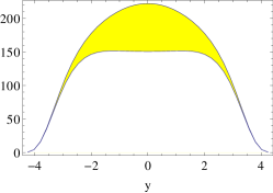
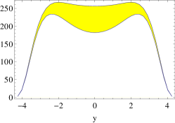
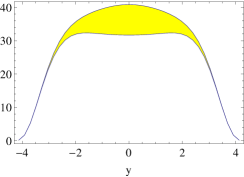
(a) $d^{2}\sigma/dM/dy$ in pb/GeV for $pp\to W^{-}+X$ (left), $pp\to W^{+}+X$ (middle) and $pp\to Z,\gamma^{*}+X$ (right) production at the LHC for 7 TeV with CTEQ6.6 using the VRAP program Anastasiou et al. (2004) at NNLO (for $M=m_{W}$ and $M=m_{Z}$ respectively).

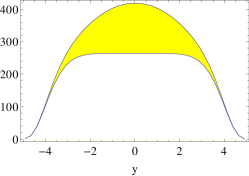
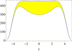
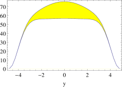
(b) $d^{2}\sigma/dM/dy$ in pb/GeV for $pp\to W^{-}+X$ (left), $pp\to W^{+}+X$ (middle) and $pp\to Z,\gamma^{*}+X$ (right) production at the LHC for 14 TeV with CTEQ6.6 using the VRAP program Anastasiou et al. (2004) at NNLO (for $M=m_{W}$ and $M=m_{Z}$ respectively).

Figure 8: Contribution of the strange quark to $W^{\pm}/Z$ production at the LHC.

Because the proton-proton LHC has a different initial state and a higher CMS energy than the Tevatron, the relative contributions of the partonic subprocesses of the $W^{\pm}/Z$ production change significantly. At the LHC, the contributions of the second generation quarks $\{s,c\}$ are greatly enhanced. Additionally, the $W^{+}$ and $W^{-}$ rapidity distributions are no longer related by a simple $y\to-y$ reflection symmetry due to the $pp$ initial state. In Figure 7 we display the contributions from the different partonic cross sections which contribute to $W^{\pm}$ and $Z$ production at LO.

Figure 7a shows the rapidity distribution at the Tevatron. For $W^{+}$ ($W^{-}$) production, the $u\bar{d}$ ($d\bar{u}$) channel (dotted black lines) contributes $90\%$ of the cross section, while in $Z$ production the $u\bar{u}$ (dotted black line) and $d\bar{d}$ (dot-dashed black line) subprocesses contribute $93\%$ of the cross section. The first generation quarks $\{u,d\}$ therefore dominate the production process while contributions from strange quarks (red dashed and blue dot-dashed lines) are comparably small with $9\%$ for $W^{\pm}$ and $5\%$ ($s\bar{s}$) for $Z$ boson production.

At the LHC, subprocesses containing strange quarks are considerably more important as shown in Fig. 7b for a CMS energy of $7$ TeV and in Fig. 7c for $14$ TeV. For $W^{-}$ production (left plots), the (blue) dot-dashed lines show the $s\bar{u}$ channel while the (red) dashed lines show the $s\bar{c}$ contribution. At $14$ TeV the $s\bar{c}\to W^{-}$ subprocess contributes $28\%$ to the cross section, while the $s\bar{u}\to W^{-}$ subprocess contributes only $2\%$ as this is suppressed by the off-diagonal CKM matrix entry. For $W^{+}$ production channels, the $\bar{s}u$ channel (blue dot-dashed lines) contributes only $2\%$, while the $\bar{s}c$ channel (red dashed lines) yields $21\%$. Notice, the absolute value of the $s\bar{c}\to W^{-}$ and $\bar{s}c\to W^{+}$ contributions are the same, however the relative contribution is smaller for $W^{+}$ production due to the larger up-quark valence contribution in the $u\bar{d}\to W^{+}$ subprocess as compared to $\bar{u}d\to W^{-}$.

The rapidity distributions of the total $W^{-}$ and $W^{+}$ boson production differ markedly at the LHC because of the different valence quark contributions from $u$ and $d$. This effect is also present in the $s\bar{u}\to W^{-}$ and $\bar{s}u\to W^{+}$ (blue dot-dashed lines) subprocess. We will comment more on this feature in the following subsection.

Comparing Figs. 7a with Figs. 7c, we note the LHC explores a much larger rapidity range. For channels containing strange quarks, $|y_{W/Z}|$ can be measured up to $y\approx 4.5$ at the LHC, compared to $y\approx 2.5$ at the Tevatron; therefore smaller values of $x$ of the strange quark distribution can be probed.

Additionally, as at the Tevatron, we can use $W^{-}$ production to probe the strange quark PDF while using $W^{+}$ production to probe the anti-strange PDF.

While the LO illustration of Fig. 7 provides a useful guide, in Fig. 8 we display the strange quark contribution to the differential cross section $d^{2}\sigma/dM/dy$ of on-shell $W^{-},\,W^{+},\,Z$ boson production computed at NNLO using the VRAP program Anastasiou et al. (2004). We display the LHC results for $W^{\pm}$ and $Z$ with $\sqrt{S}$ of both 7 TeV and 14 TeV, where the (yellow) band represents the strange-quark initiated contributions to the total differential cross section.

The figures impressively highlight the large contribution of the strange and anti-strange quark subprocesses at the LHC. Consequently it is essential to constrain the strange PDF if we are to make accurate predictions and to perform precision measurements. Figure 8 also demonstrates clearly the very different rapidity profiles of the strange quark (arising from the sea-distribution) compared to the $u$ and $d$ quark terms which are dominated by the valence distributions. This property is most evident for the case of $W^{+}$ production. Here, the dominant $u\bar{d}$ contribution has a twin-peak structure due to the harder valence distribution, while the $c\bar{s}$ distribution has a single-peak centered at $y=0$. The total distribution is then a linear combination of the twin-peak and single-peak distributions, and these are weighted by the corresponding PDF.

Therefore, a detailed measurement of the rapidity distribution of the $W^{\pm}/Z$ bosons can yield information about the contributions of the $s$ quark relative to the $u,d$ quarks. As this is a relative measurement, rather than an absolute cross section measurement, it is reasonable to expect that this could be achieved with high precision once sufficient statistics are collected. Consequently, this is an ideal measurement where the LHC data could lead to stronger constraints on the PDFs.

III.3 PDF Uncertainty of the $W/Z$ rapidity distributions

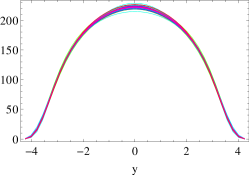
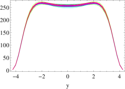
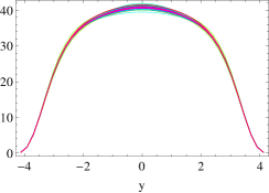
(a) $d^{2}\sigma/dM/dy$ in pb/GeV for $pp\to W^{-}+X$ (left), $pp\to W^{+}+X$ (middle) and $pp\to Z,\gamma^{*}+X$ (right) production at the LHC for 7 TeV with CTEQ6.6 using the VRAP program Anastasiou et al. (2004) at NNLO.

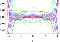
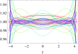
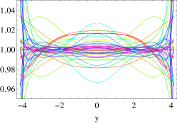
(b) $d^{2}\sigma/dM/dy$ for on-shell $\{W^{-},W^{+},Z\}$ production at the LHC for $\sqrt{S}=7$ TeV with CTEQ6.6 using the VRAP program at NNLO, scaled by the central value.

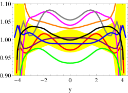
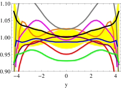
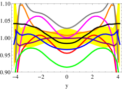
(c) $d^{2}\sigma/dM/dy$ for $\{W^{-},W^{+},Z\}$ production at the LHC for $\sqrt{S}=7$ TeV with a selection of PDFs using the VRAP program at NNLO. The (yellow) band is for the CTEQ6.6 set Nadolsky et al. (2008), and the other curves are for the central values of different PDF sets (see text). All plots are scaled by the central value for the CETQ6.6 set. Note the scale of this figure is larger than for Fig. 9b.

Figure 9: PDF uncertainty bands for on-shell $W^{-}$(left plots) , $W^{+}$(middle plots) and $Z$(right plots) production at the LHC for $\sqrt{S}=7$ TeV.

To estimate the influence of the PDF uncertainties (and in particular the strange quark PDF) on the $W/Z$ production process and its differential distributions at the LHC, we will use the different PDF sets within CTEQ6.6 as well as compare the sets of different PDF groups.

In Figure 9a, we display the differential cross section $d^{2}\sigma/dM/dy$ for $W^{\pm}/Z$ boson production at the LHC at $\sqrt{S}=7$ TeV using the 44 error PDF sets of CTEQ6.6. To better resolve these PDF uncertainties, we plot the ratio of the differential cross section $d^{2}\sigma/dM/dy$ compared to the central value in Fig. 9b. We observe that the uncertainty due to the PDFs as measured by this band is between $\pm 3\%$ and $\pm 4\%$ for central boson rapidities of $-3\leq y_{W/Z}\leq+3$. For larger rapidities, the PDF uncertainties increase dramatically, but the cross section vanishes.

For comparison, in Fig. 9c we display the (yellow) band of CTEQ6.6 error PDFs together with the results using other contemporary PDF sets. The (yellow) band shows the span of the 44 CTEQ6.6 error PDFs of Fig. 9b, and the solid lines show the rapidity distribution from the selection of PDFs; all have been scaled to the central value for the CETQ6.6 set. We observe that the choice of PDF sets can result in differences ranging up to $\pm\hskip 0.85358pt8\hskip 0.85358pt\%$ for $-2\leq y_{W/Z}\leq+2$ and even up to $\pm\hskip 0.85358pt10\hskip 0.85358pt\%$ for $-3\leq|y_{W/Z}|\leq 3$, which is well beyond the $\pm\hskip 0.85358pt3\hskip 0.85358pt\%$ and $\pm\hskip 0.85358pt4\hskip 0.85358pt\%$ range displayed in Fig. 9b; note the different scales used in Fig. 9b and Fig. 9c. However, if we compute the PDF uncertainty band using Eq. (5) as specified by Ref. Pumplin et al. (2002) we find an estimated uncertainty of $\sim 15\%$ (depending on the rapidity) which generally does encompass the range of PDFs displayed in Fig. 9c.

While the band of error PDFs provides an efficient method to quantify the uncertainty, the range spanned by the different PDF sets illustrates there are other important factors which must be considered to encompass the full range of possibilities.

III.4 Correlations of the $W/Z$ rapidity distributions

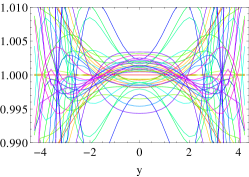
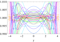
(a) Double ratio $R^{-}$ as defined in Eq. (6) for the LHC for $\sqrt{S}=7$ TeV with CTEQ6.5 (left) and CTEQ6.6 (right) at NNLO.

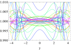
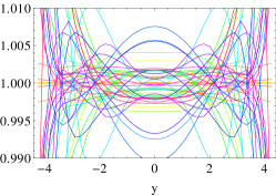
(b) Double ratio $R^{+}$ as defined in Eq. (6) for the LHC for $\sqrt{S}=7$ TeV with CTEQ6.5 (left) and CTEQ6.6 (right) at NNLO.

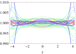
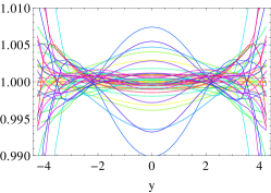
(c) Double ratio $R$ as defined in Eq. (7) for the LHC for $\sqrt{S}=7$ TeV with CTEQ6.5 (left) and CTEQ6.6 (right) at NNLO.

Figure 10: Ratios of the differential $W^{\pm}$ and $Z$ production cross section as defined in Eq. (6) and Eq. (7) at the LHC for $\sqrt{S}=7$ TeV.

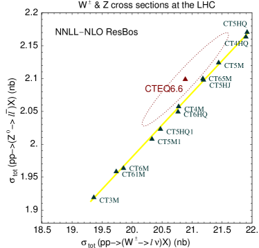
Figure 11: Correlation of the $W^{\pm}$ and $Z$ cross sections for a selection of PDF sets. Figure taken from Ref. Nadolsky et al. (2008).

The leptonic decay modes of the $W/Z$ bosons provide a powerful tool for precision measurements of electroweak parameters such as the $W$ boson mass. As the leptonic decay of the $W$ boson contains a neutrino ($W\to\ell\nu$), this process must be modeled to account for the missing neutrino. The $W$ mass can then be measured by studying the transverse momentum distribution of the decay lepton $\ell$ or the transverse mass of the $\ell\nu$ pair. Performing this measurement, the Drell-Yan $Z$ boson production process is used to calibrate the leptonic $W$ process because the $Z$ can decay into two visible leptons $Z\to\ell^{+}\ell^{-}$. This method works to the extent that the production processes of the $W$ and $Z$ bosons are correlated.

One possible measure to gauge the correlation of the PDF uncertainty is the ratio of the $W$ and $Z$ boson differential cross section. We compute $d^{2}\sigma/dM/dy$ for $W^{\pm}$ compared to $Z$, and divide by the central PDF results to see the uncertainty band on a relative scale. Schematically we define:

$$R^{\pm} = \left[\frac{d\sigma(W^{\pm})}{d\sigma(Z)}\right]/\left[\frac{d\sigma(W^{\pm})}{d\sigma(Z)}\right]_{0}$$ (6)

where the “0” subscript denotes the “central” PDF set. The resulting distributions are displayed in Fig. 10a for $W^{-}$ production and in Fig. 10b for $W^{+}$ production. The left plot in each figure shows the distributions for the CTEQ6.5 PDF set, and the right plots the distributions for CTEQ6.6. We observe that the uncertainty band is generally $\pm\hskip 0.85358pt1\hskip 0.85358pt\%$ for central rapidities of $-2\leq y_{W/Z}<+2$; this is smaller than in the previous case, where the absolute uncertainty was investigated. For larger rapidity ($\left|y_{W/Z}\right|>2$) the uncertainty band exceeds the $\pm\hskip 0.85358pt1\hskip 0.85358pt\%$ range of the plot.

In Fig. 10c, we plot the sum of the differential $W^{+}$ and $W^{-}$ cross sections with respect to the differential $Z$ boson cross section, again normalized to the distribution of the central PDF set. We define:

$$R = \left[\frac{d\sigma(W^{+}+W^{-})}{d\sigma(Z)}\right]/\left[\frac{d\sigma(W^{+}+W^{-})}{d\sigma(Z)}\right]_{0}$$ (7)

for both the CTEQ6.5 and CTEQ6.6 PDFs.

The contrast in Fig. 10c is striking. For the CTEQ6.5 PDFs, we observe that $W^{\pm}$ and $Z$ processes are strongly correlated, while for the CTEQ6.6 the spread of the PDF band is substantially larger. For example, the double ratio for CTEQ6.5 has a spread of approximately $\pm 0.2\%$ within the central rapidity range of $-3\leq y_{W/Z}\leq+3$, while the uncertainty for CTEQ6.6 is much wider in this rapidity region.

The primary difference that is driving this result is the different strange PDF. For CTEQ6.5 the strange quark was defined by Eq. (2) while CTEQ6.6 introduced two extra fitting parameters which allowed the strange PDF to vary independently from the up and down sea. Thus, the uncertainty of the CTEQ6.6 distributions more accurately reflects the true uncertainty.

Another means to see how the additional freedom of the strange quark introduces a decorrelation of the $W^{\pm}$ and $Z$ processes is evident in Fig. 11 which displays the correlation of the $W^{\pm}$ and $Z$ boson cross sections for a selection of CTEQ PDFs. Except for CTEQ6.6, all the PDFs make use of Eq. (2) and yield results that lie along a straight line in the $\{\sigma_{W},\sigma_{Z}\}$ plane. Because CTEQ6.6 does not use Eq. (2), the freedom of the strange quark PDF is reflected in the freedom of the $W^{\pm}$ and $Z$ cross sections values.

The above examples demonstrate the subtle features inherent in evaluating the PDF uncertainties. For precision measurements it is important to better constrain the parton distributions at the LHC, in particular the strange and anti-strange quark PDFs.

IV Conclusion

We have investigated the constraints of the strange and anti-strange PDFs and their impact on the Drell-Yan $W/Z$ boson production at the LHC.

Specifically, we observe that the strange quark is rather poorly constrained, particularly in the low $x$ region which is sensitive to $W/Z$ production at the LHC. Improved analyses from neutrino DIS measurements could help reduce this uncertainty. Conversely, precision measurements of $W/Z$ production at the LHC may provide input to the global PDF analyses which could further constrain these distributions.

In particular, the rapidity distribution of the $W/Z$ bosons provides an incisive measure of the mix of valence and sea quarks, and the prospect of measuring this at the LHC in the near future is excellent.

Appendix

IV.1 PDF Fits with the Dimuon Data

LO Dimuon	# pts	$B^{+}$	$A$	$B$	$C$	$B^{-}$
$[S^{-}]\times 10^{4}$	-	54.85	31.18	15.98	10.32	-17.72
Entire Data	2465	1.015 (1.100)	1.001 (1.085)	1.000 (1.084)	1.002 (1.086)	1.018 (1.103)
Dimuon	174	1.289 (0.941)	1.018 (0.743)	1.000 (0.730)	0.996 (0.727)	1.241 (0.906)
Inclusive I	194	0.978 (0.711)	0.961 (0.699)	1.000 (0.727)	1.029 (0.748)	1.085 (0.789)
Dimuon+I	368	1.126 (0.820)	0.989 (0.720)	1.000 (0.728)	1.014 (0.738)	1.160 (0.844)
Inclusive II	2097	1.012 (1.120)	1.014 (1.123)	1.000 (1.107)	1.011 (1.119)	1.011 (1.119)

Table 2: Fit results using the LO dimuon calculation. We present the integrated strange-quark asymmetry $[S^{-}]$, and the cells display $\chi^{2}/\chi_{0}^{2}$, and the values in parentheses are the $\chi^{2}/DoF$ for each data subset. Note $\chi_{0}^{2}$ is calibrated from the LO $B$-fit.

NLO Dimuon	# pts	$B^{+}$	$A$	$B$	$C$	$B^{-}$
$[S^{-}]\times 10^{4}$	-	63.75	23.92	13.72	12.81	-18.59
Entire Data	2465	1.033 (1.120)	0.995 (1.079)	0.994 (1.077)	0.994 (1.077)	1.025 (1.111)
Dimuon	174	1.660 (1.212)	0.960 (0.701)	0.936 (0.683)	0.937 (0.684)	1.416 (1.034)
Inclusive I	194	0.977 (0.710)	0.974 (0.708)	1.008 (0.733)	1.017 (0.739)	1.088 (0.791)
Dimuon+I	368	1.301 (0.947)	0.968 (0.705)	0.974 (0.709)	0.979 (0.713)	1.245 (0.906)
Inclusive II	2097	1.012 (1.120)	1.009 (1.117)	1.007 (1.115)	1.005 (1.113)	1.010 (1.118)

Table 3: Fit results using the NLO dimuon calculation. We present the integrated strange-quark asymmetry $[S^{-}]$, and the cells display $\chi^{2}/\chi_{0}^{2}$, and the values in parentheses are the $\chi^{2}/DoF$ for each data subset.

We have repeated the LO analysis of Ref. Olness et al. (2005) and extended this using the NLO calculation for dimuon production Kretzer and Schienbein (1998); Kretzer et al. (2002). We have performed a series of fits to the data which includes the dimuon data. The results of the $\{A,B^{+},B,B^{-},C\}$ fits using the LO dimuon analysis are shown in Table 2, and those with the NLO analysis are in Table 3. The fits are sorted left-to-right by the integrated strange-quark asymmetry $[S^{-}]$ (scaled by $10^{4}$). The cells display the $\chi^{2}$ relative to $\chi_{0}^{2}$ for the indicated data set where we choose $\chi_{0}^{2}$ to be the $\chi^{2}$ value from the LO-$B$ fit; this allows us to compare the incremental changes as we shift $[S^{-}]$ and alter the constraints. The values in parentheses are the $\chi^{2}/DoF$ for each data subset. The $B$-fit is the overall best fit to the data. The $B^{+}$ and $B^{-}$ sets modify the $B$ fit using the Lagrange multiplier method to determine the ranges of the $[S^{-}]$ parameter defined in Eq. (3).

For example, the LO $B^{+}$ fit demonstrates that we can increase $[S^{-}]$ from 15.98 to 54.85, but the dimuon $\chi^{2}$ increases by $33/174\sim 21\%$ while the overall $\chi^{2}$ increases by only $39/2465\sim 2\%$; thus, the shift of $[S^{-}]$ is strongly constrained by the dimuon data, and the remaining data are relatively insensitive to this quantity.

Comparing the NLO-$B$ fit to the LO-$B$ fit we note that $\chi^{2}/DoF$ has decreased both for the dimuon set and the entire data set; while this decrease is not dramatic, it is encouraging to see that the proper NLO treatment of the data results in an improved fit. As before, we observe that for the NLO $B^{+}$ fit, we can increase $[S^{-}]$ from 13.72 to 63.75, but the dimuon $\chi^{2}$ increases by $92/174\sim 53\%$ while the overall $\chi^{2}$ increases by only $106/2465\sim 4\%$; again, the shift of $[S^{-}]$ is primarily constrained by the dimuon data.

In Figure 2 we have plotted the ratio $\chi^{2}/\chi_{0}^{2}$ for the individual dimuon and “Inclusive-I” data sets Olness et al. (2005) evaluated for a series of NLO $B$-fits as a function of the strange asymmetry $[S^{-}]\times 10^{4}$. This plot allows us to see the contribution of each data set as we shift the strange asymmetry. Again the “Inclusive-I” data sets are essentially unchanged as the treatment of the dimuons only affects these data indirectly. As before, this data set is mildly sensitive to the dimuons, and weakly prefers larger values of $[S^{-}]$.

References

- Abramowicz et al. (1982) H. Abramowicz et al., Z. Phys. C15, 19 (1982).
- Abramowicz et al. (1983) H. Abramowicz et al., Z. Phys. C17, 283 (1983).
- Abramowicz et al. (1984) H. Abramowicz et al., Z. Phys. C25, 29 (1984).
- Berge et al. (1987) J. P. Berge et al., Z. Phys. C35, 443 (1987).
- Aivazis et al. (1994) M. A. G. Aivazis, J. C. Collins, F. I. Olness, and W.-K. Tung, Phys. Rev. D50, 3102 (1994), eprint hep-ph/9312319.
- Bazarko et al. (1995) A. Bazarko et al. (CCFR Collaboration), Z.Phys. C65, 189 (1995), eprint hep-ex/9406007.
- Gluck et al. (1996) M. Gluck, S. Kretzer, and E. Reya, Phys.Lett. B380, 171 (1996), erratum-ibid. B405 (1997) 391, eprint hep-ph/9603304.
- Alton et al. (2001) A. Alton et al. (NuTeV Collaboration), Int.J.Mod.Phys. A16S1B, 764 (2001), eprint hep-ex/0008068.
- Goncharov et al. (2001) M. Goncharov et al. (NuTeV Collaboration), Phys.Rev. D64, 112006 (2001), eprint hep-ex/0102049.
- Kretzer et al. (2004) S. Kretzer, H. L. Lai, F. I. Olness, and W. K. Tung, Phys. Rev. D69, 114005 (2004), eprint hep-ph/0307022.
- Nadolsky et al. (2003) P. M. Nadolsky, N. Kidonakis, F. I. Olness, and C. P. Yuan, Phys. Rev. D67, 074015 (2003), eprint hep-ph/0210082.
- Pumplin et al. (2002) J. Pumplin et al., JHEP 07, 012 (2002), eprint hep-ph/0201195.
- Spentzouris (2002) P. Spentzouris (NuTeV), Acta Phys. Polon. B33, 3843 (2002).
- Tung et al. (2002) W.-K. Tung, S. Kretzer, and C. Schmidt, J. Phys. G28, 983 (2002), eprint hep-ph/0110247.
- Tzanov et al. (2005) M. Tzanov et al. (NuTeV), Int. J. Mod. Phys. A20, 3759 (2005).
- Tzanov et al. (2006) M. Tzanov et al. (NuTeV), Phys. Rev. D74, 012008 (2006), eprint hep-ex/0509010.
- Adams et al. (2010) T. Adams et al. (NuSOnG), Int. J. Mod. Phys. A25, 909 (2010), eprint 0906.3563.
- Stump et al. (2003) D. Stump, J. Huston, J. Pumplin, W.-K. Tung, H. Lai, et al., JHEP 0310, 046 (2003), eprint hep-ph/0303013.
- Nadolsky et al. (2008) P. M. Nadolsky, H.-L. Lai, Q.-H. Cao, J. Huston, J. Pumplin, et al., Phys.Rev. D78, 013004 (2008), eprint 0802.0007.
- Martin et al. (2009) A. Martin, W. Stirling, R. Thorne, and G. Watt, Eur.Phys.J. C63, 189 (2009), eprint 0901.0002.
- Ball et al. (2010) R. D. Ball et al., Nucl. Phys. B838, 136 (2010), eprint 1002.4407.
- Alekhin et al. (2010) S. Alekhin, J. Blumlein, S. Klein, and S. Moch, Phys.Rev. D81, 014032 (2010), eprint 0908.2766.
- Jimenez-Delgado and Reya (2009) P. Jimenez-Delgado and E. Reya, Phys.Rev. D79, 074023 (2009), eprint 0810.4274.
- Mason et al. (2007) D. Mason et al. (NuTeV Collaboration), Phys.Rev.Lett. 99, 192001 (2007).
- Zeller et al. (2002) G. Zeller et al. (NuTeV Collaboration), Phys.Rev. D65, 111103 (2002), eprint hep-ex/0203004.
- Yang et al. (2001) U.-K. Yang et al. (CCFR/NuTeV Collaboration), Phys.Rev.Lett. 86, 2742 (2001), eprint hep-ex/0009041.
- Olness et al. (2005) F. Olness, J. Pumplin, D. Stump, J. Huston, P. M. Nadolsky, et al., Eur.Phys.J. C40, 145 (2005), eprint hep-ph/0312323.
- Airapetian et al. (2008) A. Airapetian et al. (HERMES), Phys. Lett. B666, 446 (2008), eprint 0803.2993.
- Onengut et al. (2004) G. Onengut et al. (CHORUS), Phys. Lett. B604, 11 (2004).
- Onengut et al. (2006) G. Onengut et al. (CHORUS), Phys. Lett. B632, 65 (2006).
- Kayis-Topaksu et al. (2008) A. Kayis-Topaksu et al. (CHORUS), Nucl. Phys. B798, 1 (2008), eprint 0804.1869.
- Owens et al. (2007) J. Owens, J. Huston, C. Keppel, S. Kuhlmann, J. Morfin, et al., Phys.Rev. D75, 054030 (2007), eprint hep-ph/0702159.
- Astier et al. (2000) P. Astier et al. (NOMAD), Phys. Lett. B486, 35 (2000).
- Petti (2006) R. Petti (NOMAD), Nucl. Phys. Proc. Suppl. 159, 56 (2006), eprint hep-ex/0602022.
- Wu et al. (2008) Q. Wu et al. (NOMAD), Phys. Lett. B660, 19 (2008), eprint 0711.1183.
- de Florian and Sassot (2004) D. de Florian and R. Sassot, Phys.Rev. D69, 074028 (2004), eprint hep-ph/0311227.
- Hirai et al. (2007) M. Hirai, S. Kumano, and T.-H. Nagai, Phys.Rev. C76, 065207 (2007), eprint 0709.3038.
- Eskola et al. (2009) K. Eskola, H. Paukkunen, and C. Salgado, JHEP 0904, 065 (2009), eprint 0902.4154.
- Schienbein et al. (2008) I. Schienbein, J. Yu, C. Keppel, J. Morfin, F. Olness, et al., Phys.Rev. D77, 054013 (2008), eprint 0710.4897.
- Schienbein et al. (2009) I. Schienbein et al., Phys. Rev. D80, 094004 (2009), eprint 0907.2357.
- Kovarik et al. (2011a) K. Kovarik et al., Phys. Rev. Lett. 106, 122301 (2011a), eprint 1012.0286.
- Kovarik et al. (2011b) K. Kovarik et al. (2011b), eprint 1111.1145.
- Kovarik et al. (2011c) K. Kovarik et al., AIP Conf. Proc. 1369, 80 (2011c).
- Aaltonen et al. (2008) T. Aaltonen et al. (CDF Collaboration), Phys.Rev.Lett. 100, 091803 (2008), eprint 0711.2901.
- Abazov et al. (2008) V. Abazov et al. (D0 Collaboration), Phys.Lett. B666, 23 (2008), eprint 0803.2259.
- Kawamura et al. (2011) H. Kawamura, S. Kumano, and Y. Kurihara, Phys.Rev. D84, 114003 (2011), eprint 1110.6243.
- Besson et al. (2008) N. Besson, M. Boonekamp, E. Klinkby, S. Mehlhase, and T. Petersen (ATLAS Collaboration), Eur.Phys.J. C57, 627 (2008), eprint 0805.2093.
- Krasny et al. (2010) M. W. Krasny, F. Dydak, F. Fayette, W. Placzek, and A. Siodmok, Eur. Phys. J. C69, 379 (2010), eprint 1004.2597.
- Chatrchyan et al. (2011a) S. Chatrchyan et al. (CMS Collaboration), Phys.Rev. D84, 112002 (2011a), eprint 1110.2682.
- Tarrade (2011) F. Tarrade, Tech. Rep. ATL-PHYS-PROC-2011-003, CERN, Geneva (2011).
- Chatrchyan et al. (2011b) S. Chatrchyan et al. (CMS Collaboration), JHEP 1108, 117 (2011b), eprint 1104.1617.
- Ball et al. (2011a) R. D. Ball et al. (NNPDF Collaboration), Phys.Lett. B704, 36 (2011a), eprint 1102.3182.
- Peskin and Takeuchi (1992) M. E. Peskin and T. Takeuchi, Phys.Rev. D46, 381 (1992).
- Dittmar et al. (1997) M. Dittmar, F. Pauss, and D. Zurcher, Phys.Rev. D56, 7284 (1997), eprint hep-ex/9705004.
- Alekhin et al. (2011) S. Alekhin, J. Blumlein, P. Jimenez-Delgado, S. Moch, and E. Reya, Phys.Lett. B697, 127 (2011), eprint 1011.6259.
- Blumlein et al. (2011) J. Blumlein, A. Hasselhuhn, P. Kovacikova, and S. Moch, Phys.Lett. B700, 294 (2011), eprint 1104.3449.
- Alekhin et al. (2012) S. Alekhin, J. Blumlein, and S. Moch (2012), eprint 1202.2281.
- Aad et al. (2011) G. Aad et al. (ATLAS Collaboration) (2011), eprint 1109.5141.
- Aad et al. (2012) G. Aad et al. (ATLAS Collaboration) (2012), eprint 1203.4051.
- Chatrchyan et al. (2011c) S. Chatrchyan et al. (CMS Collaboration) (2011c), eprint 1110.4973.
- Chatrchyan et al. (2011d) S. Chatrchyan et al. (CMS Collaboration), JHEP 1110, 132 (2011d), eprint 1107.4789.
- (2011a) (CMS Collaboration), CMS-PAS-EWK-10-011 (2011a).
- (2011b) (CMS Collaboration), CMS-PAS-EWK-11-005 (2011b).
- Chatrchyan et al. (2011e) S. Chatrchyan et al. (CMS Collaboration), JHEP 1104, 050 (2011e), eprint 1103.3470.
- Amhis, Yasmine et al. (2012) Amhis, Yasmine et al. (LHCb Collaboration) (2012), eprint 1202.0654.
- Shears (2011) T. Shears (LHCb Collaboration), LHCb-Proc-2011-076 (2011).
- (2011c) (CMS Collaboration), CMS-PAS-EWK-11-013 (2011c).
- Anastasiou et al. (2004) C. Anastasiou, L. J. Dixon, K. Melnikov, and F. Petriello, Phys.Rev. D69, 094008 (2004), eprint hep-ph/0312266.
- Ball et al. (2011b) R. D. Ball, V. Bertone, F. Cerutti, L. Del Debbio, S. Forte, et al., Nucl.Phys. B849, 296 (2011b), eprint 1101.1300.
- Lai et al. (2010) H.-L. Lai, M. Guzzi, J. Huston, Z. Li, P. M. Nadolsky, et al., Phys.Rev. D82, 074024 (2010), eprint 1007.2241.
- Tung et al. (2007) W. Tung, H. Lai, A. Belyaev, J. Pumplin, D. Stump, et al., JHEP 0702, 053 (2007), eprint hep-ph/0611254.
- Aaron et al. (2010) F. Aaron et al. (H1 and ZEUS Collaboration), JHEP 1001, 109 (2010), eprint 0911.0884.
- Martin et al. (2004) A. Martin, R. Roberts, W. Stirling, and R. Thorne, Phys.Lett. B604, 61 (2004), eprint hep-ph/0410230.
- Kretzer and Schienbein (1998) S. Kretzer and I. Schienbein, Phys. Rev. D58, 094035 (1998), eprint hep-ph/9805233.
- Kretzer et al. (2002) S. Kretzer, D. Mason, and F. Olness, Phys.Rev. D65, 074010 (2002), eprint hep-ph/0112191.