A new layout optimization technique for interferometric arrays and the final MWA antenna layout

Abstract

Antenna layout is an important design consideration for radio interferometers because it determines the quality of the snapshot point spread function (PSF, or array beam). This is particularly true for experiments targeting the 21 cm Epoch of Reionization signal as the quality of the foreground subtraction depends directly on the spatial dynamic range and thus the smoothness of the baseline distribution. Nearly all sites have constraints on where antennas can be placed—even at the remote Australian location of the MWA (Murchison Widefield Array) there are rock outcrops, flood zones, heritages areas, emergency runways and trees. These exclusion areas can introduce spatial structure into the baseline distribution that enhance the PSF sidelobes and reduce the angular dynamic range. In this paper we present a new method of constrained antenna placement that reduces the spatial structure in the baseline distribution. This method not only outperforms random placement algorithms that avoid exclusion zones, but surprisingly outperforms random placement algorithms without constraints to provide what we believe are the smoothest constrained baseline distributions developed to date. We use our new algorithm to determine the final antenna placement for the MWA, and present the planned antenna locations, baseline distribution, and snapshot PSF for the observatory.

1 Introduction

Antenna placement is a critical design criterion for any interferometric array as it determines the baseline distribution and thus the angular dynamic range of the point spread function of the observatory. Nearly all observatory sites have areas where antennas cannot be placed. Buildings, roads, runways, power and data access, land use and ownership issues, endangered flora and fauna, flood zones, elevation, and ground stability are but a few of the common issues that constrain the placement of antennas. Even in remote desert locations a flat and barren terrain can quickly become dotted with exclusion zones where antennas cannot be placed.

This is of particular concern for 21 cm Cosmology telescopes targeting the Epoch of Reionization (EoR) and Baryon Acoustic Oscillation (BAO) dark energy measurements, as the quality of the monochromatic PSF is directly related to the ability to subtract foreground contamination (Morales et al., 2006; Datta et al., 2011; Liu & Tegmark, 2011; Bernardi et al., 2011, Vedantham, Shankar, Subrahmanyan in review). Antenna exclusion zones can introduce asymmetries in the baseline distribution which limit the angular dynamic range and thus achievable level of foreground subtraction (see Morales & Wyithe, 2010, for a recent review of foreground subtraction for 21 cm Cosmology).

There is a long history of array configuration studies, including optimization of arrays with cost constraints (e.g.  Cohanim et al., 2010), simulated annealing for small $N$ arrays (Cornwell, 1988), optimization to reduce the peak sidelobe levels (Kogan, 2000, Kogan & Cohen 2005, LWA Memo 21), or optimization to match a particular baseline distribution with and without ground constraints (Boone, 2001, Lal et al. SKA Memo 107). Our particular concern is situations in which some areas cannot be used (exclusion zones), a particular radial baseline distribution must be met, and a very high angular dynamic range must be achieved. While our problem is similar to that of Boone (2001), we find that the figure of merit used in that work does not sufficiently capture large scale structure in the baseline distribution. We develop an alternative figure of merit, which naturally leads to a new optimization method.

In §2 we explore the effect of exclusion zones on the baseline distribution, develop a new spatially sensitive figure of merit, and present our new optimization method. We then apply our method to placing the MWA tiles in §3, and present the final MWA antenna configuration. The locations of all 512 tiles are provided in the electronic supplement.

2 Array Layout Comparisons and a new technique

Proposed and future large $N$ radio arrays will face the challenge of placing hundreds to thousands of antennas to optimize scientific goals, while obeying numerous constraints. While most physical constraints exist on the antenna locations (areas of exclusion on the ground), science capabilities are optimized in the uv plane for an interferometric measurement, and hence these arrays should match the ideal baseline distribution as closely as possible. This makes the problem very non-linear because any one antenna placement affects $N-1$ baselines, and it is not immediately obvious how a constraint such as an exclusion area will affect the baseline distribution.

In our analysis, we explored three array layout methods. The first method is random and with no exclusion areas (“random unmasked”), in which antennas are placed randomly with a weighted radial distribution. Algorithmically, for each antenna a radius is first drawn from a distribution that matches the desired radial density profile, then azimuthal angles are chosen at random until one is found that does not overlap with previously placed antennas. The second array generation method is also random but incorporates exclusion areas (“random masked”). This method is identical to the random unmasked method, with the addition of avoiding exclusion areas by the use of a mask that is checked in the same step as checking for overlap with previous tiles. The third and final method is the algorithm that we developed (“active method”), that actively minimizes spatial structure in the baseline distribution and is detailed later in this section. Our analysis assumes the scientifically desired uv or antenna distribution is known. We use the specifications for the MWA telescope (which are described in §3), but our methods are generalizable to any large $N$ array.

Figure 1 shows three examples of baseline distributions generated by the random unmasked, random masked, and active masked methods respectively. The left pane shows the baseline distribution on a logarithmic scale, while the right pane shows the difference from the ideal smooth analytic function to accentuate undesired structures in the uv distributions. These three examples are representative of the over four thousand array layouts we have hand graded to arrive at our conclusions.

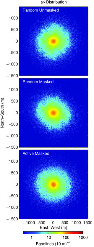
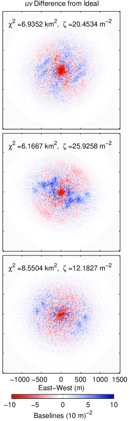
Figure 1: Example uv distributions for array layouts generated by (top to bottom) the random unmasked, random masked, and active masked methods. The left panes show the snapshot single frequency baseline distributions on a log scale, while the right panes show the difference of this distribution from the smooth analytic ideal. The small scale fuzzy noise is equally present in all array realizations and is due to the finite number of antennas. However, the large scale structure varies greatly from array to array. The exclusion areas have introduced significant asymmetries in the baseline distribution of the random masked method (middle row). The active masked method (bottom row) is able to highly suppress this structure, even beyond the level of the unconstrained random method (top row). Furthermore, we see the figure of merit, $\zeta$, accurately reflects the amount of azimuthal structure in the distributions (see Figure 2).

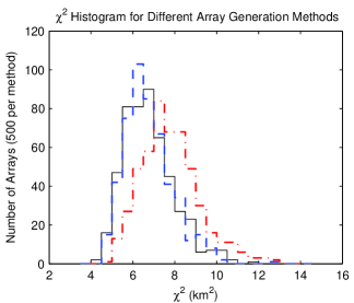
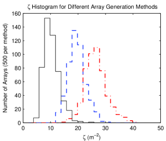
Figure 2: $\chi^{2}$ and $\zeta$ histograms for random unmasked, random masked, and active masked methods as denoted by the thick dashed blue, thick dot-dashed red, and thin solid black lines respectively. While the $\chi^{2}$ values do not distinguish the quality of the different realizations (a conclusion firmly supported by our hand grading), the $\zeta$ values strongly separate the realizations based on asymmetry.

All of these images have fuzzy small scale noise due to the finite number of antennas. However, there is another more insidious artifact present in the masked baseline distribution (middle row of Figure 1)—large scale structure imprinted by the antenna exclusion areas. In all of the masked random array realizations there are significant regions of over and under densities in the baseline distribution which translate directly into unwanted PSF features.

To understand the effect of baseline over and under densities, consider a nearly perfect uv distribution with a small region of excess baselines. This region of uv over density can be viewed as a ‘wave packet’ of baselines at similar spatial frequencies. In the wave packet picture there is a fundamental corrugation in the PSF given by the location of the center of the excess region. However, the nearby modes in the packet beat in and out of phase with the fundamental corrugation. When the wave numbers are all in phase the amplitude is very high—the number of excess baselines in the region—but they quickly dephase only to rephase again some distance further along in the PSF. The undesirable ‘features’ seen in most PSFs are the periodic signature of a wavepacket beating across the PSF. Over (or under) dense regions that cover a large portion of the uv plane will quickly damp down (wide bandwidth), though they often have a lot of power due to the large number of baselines involved, and correspond to large close-in sidelobes. Smaller features in the uv plane damp more slowly and repeat many times across the PSF leading to the small far sidelobes. A smooth uv distribution necessarily leads to a smooth PSF, and the PSF slidelobe structure is dominated not by the unavoidable fuzzy noise but instead the larger regions of over and under density in the uv plane.

Our first approach to quantify the deviations from the desired uv distributions was to consider $\chi^{2}$. This was calculated by gridding the uv distribution and integrating the square of the difference from the ideal, weighted by the variance in each pixel from 500 random unmasked realizations. However, $\chi^{2}$ is not a spatially aware function—any deviation from the ideal is weighted the same regardless of where in the uv plane the deviation occurs. Because of this lack of spatial information, $\chi^{2}$ does not capture the large scale structure that is important to choosing an array. The examples in Figure 1 vary quite a bit in quality, however, the associated $\chi^{2}$ values do not reliably reflect the degree of spatial structure. The insensitivity of $\chi^{2}$ to array quality is demonstrated again in the histogram in Figure 2. Despite a clear qualitative difference between the masked and unmasked random configurations (dashed blue and dash-dot red) the distributions of $\chi^{2}$ are very similar.

With the spatial dependence in mind, our next step was to develop a figure of merit based on a Bessel decomposition. The residual uv distribution ($D(r,\phi)$, difference between actual and desired) can be decomposed into Bessel modes

$$D(r,\phi)=\sum_{n=1}^{\infty}\sum_{m=0}^{\infty}J_{m}\left(\frac{x_{mn}r}{R}\right)(A_{mn}\sin(m\phi)+B_{mn}\cos(m\phi)),$$ (1)

where $x_{mn}$ is the $n^{\rm th}$ zero of the $m^{\rm th}$ Bessel function. The amplitudes of the asymmetric Bessel coefficients ($A_{mn},\ B_{mn},\ m>0$) reflect the asymmetric spatial over and under densities in the uv plane. We then define a figure of merit $\zeta$ as the sum of these Bessel coefficients

$$\zeta\equiv\sum_{m>0,n}^{{\rm max\ }m,n}\sqrt{A_{mn}^{2}+B_{mn}^{2}}.$$ (2)

Smaller $\zeta$ corresponds to less spatial structure, and hence a more desirable layout. The right hand panel of Figure 2 shows the $\zeta$ distributions for the same arrays, clearly separating the masked and unmasked random arrays, and in Figure 1 the $\zeta$ values accurately track the quality of the array realizations.

To minimize our figure of merit, we created an active masked algorithm based on the $\zeta$ figure of merit. For computational reasons we first place a subset of the antennas (350 of 496 for our example) using the random masked method. Then for each remaining antenna, we first choose a weighted random radius, $r$, and many candidate azimuthal locations (angular spacing of 10 m in our example). We then select the location with the smallest $\zeta$ value, and repeat until all $N$ antennas are placed.

The result is clear in Figures 1 & 2. Despite having the additional constraint of the exclusion areas, the active masked method produces more symmetric baseline distributions than either the random masked (expected) or random unmasked methods (unexpected). We can see this qualitatively by comparing the baseline distributions in the three examples. In the thousands of arrays we examined by hand we observed a very strong correlation between small $\zeta$ and spatial symmetry . The success of our algorithm is shown statistically by the distribution of $\zeta$ values for the three methods in Figure 2.

It is of interest to note that significant baseline asymmetry arises even in the unmasked random array realizations (Figure 1 top row, no exclusion areas). These asymmetries are due to shot noise in the random antenna placement. Conceptually, as the last few antennas are added images of the entire array are added to the uv plane at that distance from the center. For centrally condensed arrays this can produce lumps in the uv plane. Alternatively, one can consider moving a single antenna on the ground which coherently changes $N-1$ baselines. Small random associations can thus make significant correlations in the baseline distribution.

The new active method based on the Bessel decomposition figure of merit produces arrays which are superior to even an unconstrained random algorithm, even in the face of significant exclusion areas.

3 MWA Final Layout

We have used our new algorithm to determine the final array layout of the MWA. The full build out of the MWA will consist of 512 “tiles” (each comprised of 16 radio dipoles). The majority of the tiles (496) will be distributed over a 1.5 km diameter core, with the remaining 16 tiles at a $\sim$3 km diameter to provide higher angular resolution for solar measurements. The 16 “outliers” are placed by hand, while we implement our algorithm for the 496 core tiles. The tile density distribution will be constant within a central 50m radius, and have a $r^{-2}$ dependence beyond (see Lonsdale et al., 2009, for a full description of the MWA instrument). The smooth ideal distribution is shown in Figure 3.

Figure 3: MWA ideal uv distribution. This distribution was used in the active masked method for generating the final MWA layout. Compare to top left pane of Figure 5

Several parameters of the algorithm were explored to further improve the quality of the arrays being generated. For example, we varied the number of random tiles placed before initializing the active phase of our algorithm. We found that placing 350 random tiles provided sufficiently unconstrained initial conditions to proceed with the active phase. Running the algorithm in this mode 500 times provided a good sampling of the phase space.

We also investigated several array center locations within a few hundred meters of the nominal array location. Due to the irregular distribution of avoidance areas on the ground, choosing different centers did have an effect on the quality of the best arrays generated by our algorithm. In particular, a center near a high concentration of vegetation or rock outcrops usually results in a deficit of short baselines. We used this information, along with feedback from a ground truth survey in February 2011 to determine our final array center.

After generating 500 candidate arrays for each potential location, we used $\zeta$ as a guideline for selecting the highest quality array layouts, backed by hand grading. The result is the final location and layout of the MWA. Figure 6 shows an illustration the final array overlaid on an aerial photo of the site. The locations of 496 core tiles, along with the 16 hand placed outliers, are available in the electronic supplement to this paper. Figures 4 & 5 show the corresponding uv distribution and PSF. There is essentially no asymmetry in the final array—all of the large scale structure is greatly suppressed, providing a very smooth uv sampling. The small residual ripples in the PSF are on the order of the background noise we expect due to the finite number of tiles. Following the discussion of Morales (2005) and using the parameters from Bowman et al. (2006), the thermal noise uncertainty on the EoR power spectrum can be calculated in the bottom panel of Figure 4. With the exception of the small deviation at very low $k$, the thermal noise for our proposed layout very nearly traces that of the ideal array.

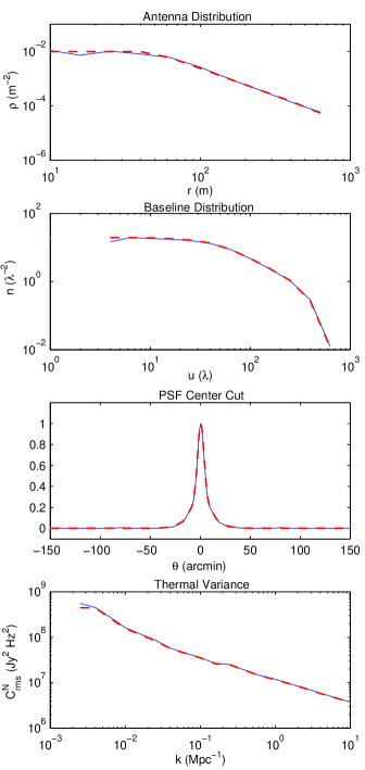
Figure 4: In each figure the final MWA array layout (thin solid blue) is compared to the analytic ideal baseline distribution (thick dashed red). Top to bottom these are the radial antenna distribution, the radial baseline distribution, a cut through the snapshot single frequency PSF, and the thermal noise as a function of cosmological wavenumber $k$ for a fiducial EoR measurement (following Bowman et al., 2006). In all aspects the final array very nearly traces the ideal array.

4 Conclusions

While we have been motivated by the need to generate a final array configuration for the MWA with exquisite smoothness in the PSF despite significant exclusion areas, we hope our method will be useful for determining the antenna layouts of other large $N$ arrays. In particular we have developed a new figure of merit based on Bessel decomposition that is sensitive to large scale over and under densities in the uv plane. We have shown that algorithms based on this figure of merit can achieve extremely smooth baseline distributions while avoiding areas where antennas cannot be placed.

We have used this new algorithm to choose the final antenna locations of the MWA. The first construction stage of the MWA will consist of $\sim$128 antenna subsample of the array configuration shown in this paper.

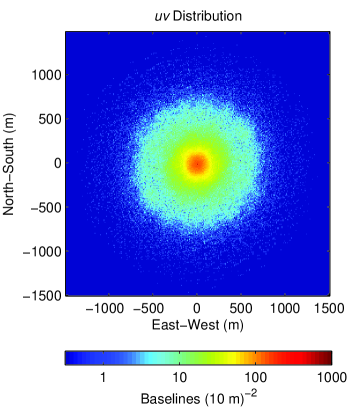
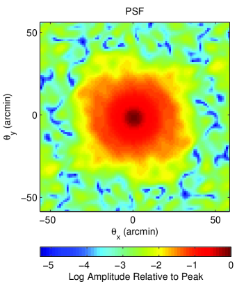
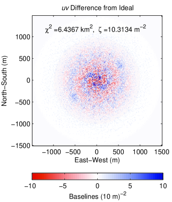
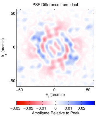
Figure 5: Baseline distribution and point spread function of proposed MWA array layout. The baseline distribution is shown in the left column, with the difference from ideal on the bottom. The azimuthal structure is nearly completely suppressed, and only small scale noise remains. The snapshot PSF for 150 MHz at zenith is shown in the right column. The sensitivity relative to the peak is shown on the top, while the difference from ideal is on the bottom. The residual ripples in the PSF difference are $\approx 1\%$ of the peak, which is on order with the background ripples expected due to our finite number of tiles.

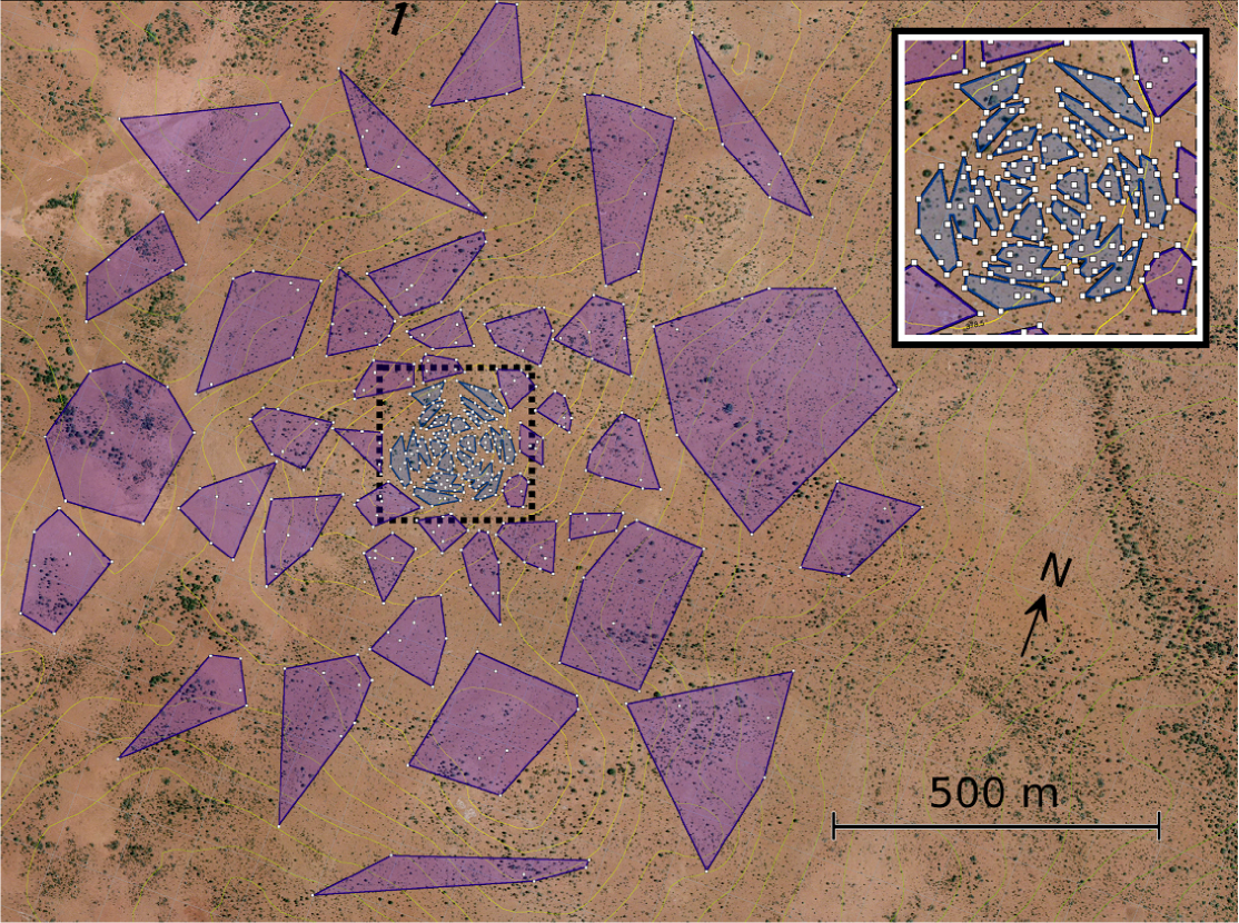
Figure 6: An aerial photo of the MWA site with the final 496 tile core array superimposed. White squares represent tiles (to scale). The colored polygons depict a possible receiver scheme. Each polygon outlines a receiver set’s electrical footprint (8 tiles per polygon except for a few outer receiver sets that will service some of the 16 outlier tiles not shown here). Inset: An enlarged view of the center of the array.

Table 1: List of tile locations for 512 tile MWA layout. The locations listed are in meters East and North relative to the center of the array at -26^∘ 42’ 4.77521” latitude, 116^∘ 40’ 11.39333” longitude. The first 496 tiles were placed using our algorithm described in the paper, while the final 16 tiles were placed by hand to optimize solar measurements.

Tile Number	East (m)	North (m)	Tile Number	East (m)	North (m)	Tile Number	East (m)	North (m)
0	58.39	175.52	54	102.43	21.22	108	162.64	199.62
1	-66.83	-117.18	55	622.87	317.32	109	35.21	48.62
2	4.47	-44.18	56	-153.15	82.42	110	12.78	-36.28
3	-22.48	27.72	57	58.24	-4.48	111	-65.47	-159.48
4	-139.89	-49.88	58	-8.72	77.52	112	-15.83	156.72
5	105.98	-16.38	59	46.77	-75.08	113	119.55	-3.68
6	275.71	-257.68	60	-375.14	-116.48	114	91.21	162.32
7	149.63	-188.58	61	-144.67	65.82	115	-9.19	-73.78
8	-589.30	-12.68	62	-6.06	-127.28	116	-45.47	79.32
9	-554.53	-344.68	63	299.67	-25.78	117	164.78	103.42
10	-235.98	-97.48	64	-85.48	203.32	118	9.21	43.42
11	-202.84	-39.38	65	133.51	59.12	119	-57.29	-35.28
12	8.98	-73.28	66	-16.48	-1.08	120	16.03	-82.58
13	10.81	-453.68	67	52.52	-48.98	121	-71.08	-110.78
14	-251.45	-280.98	68	-45.67	24.92	122	94.94	-47.98
15	187.90	-303.28	69	-374.81	149.52	123	-41.68	-54.48
16	-73.07	-62.18	70	-536.54	-393.88	124	92.05	11.82
17	53.00	-12.58	71	-100.44	-33.78	125	119.60	-58.08
18	35.23	40.42	72	-67.48	-85.88	126	-72.90	-8.68
19	304.98	38.42	73	-102.84	-16.58	127	102.10	-38.68
20	11.82	579.82	74	-251.57	199.12	128	-480.41	190.32
21	10.79	-61.58	75	-62.64	329.32	129	38.20	-33.48
22	127.63	50.52	76	-308.45	-197.68	130	133.19	-625.88
23	31.51	-20.58	77	-137.03	210.92	131	43.30	-24.78
24	-207.94	205.52	78	8.14	-98.08	132	-6.34	-49.08
25	-56.64	-60.78	79	-119.61	369.12	133	153.68	99.92
26	486.42	29.52	80	24.37	55.52	134	-11.34	193.62
27	84.02	3.02	81	-92.41	73.82	135	-25.52	-13.88
28	79.49	-20.38	82	-84.08	107.32	136	-219.04	377.02
29	12.74	-23.78	83	-5.86	-338.28	137	-557.56	-82.48
30	-251.19	-107.18	84	-393.68	-59.68	138	-437.25	-64.28
31	-18.84	-17.38	85	-313.56	151.22	139	-29.22	52.92
32	634.18	-316.28	86	-13.62	28.12	140	228.82	195.52
33	-471.65	-481.98	87	-35.07	17.82	141	80.32	50.72
34	125.53	133.62	88	-163.21	667.92	142	-81.27	119.62
35	0.58	17.52	89	102.92	-27.98	143	29.77	134.92
36	-9.60	11.42	90	-32.97	127.02	144	-489.19	-325.98
37	-42.31	-3.08	91	406.40	-257.48	145	72.61	40.52
38	-40.26	-86.18	92	71.57	-0.78	146	-313.32	-630.98
39	-48.87	9.02	93	141.42	-50.78	147	-22.83	2.92
40	-69.61	76.42	94	99.90	-282.68	148	-26.87	-79.58
41	-9.85	-6.18	95	-490.87	-357.48	149	-32.06	-41.28
42	148.65	18.52	96	63.70	-52.68	150	-79.71	557.82
43	1.20	-0.68	97	-0.24	-54.48	151	-287.67	-44.38
44	-20.88	11.32	98	-262.10	356.82	152	297.58	49.62
45	354.74	-588.58	99	38.24	-14.08	153	-21.16	-195.28
46	61.22	-35.98	100	17.18	-1.68	154	56.35	104.72
47	-648.61	298.82	101	74.05	-146.08	155	-281.52	-163.38
48	-66.65	-140.18	102	234.14	137.32	156	30.55	-37.88
49	28.34	-7.58	103	47.76	40.02	157	96.44	130.42
50	103.83	-106.78	104	-165.60	27.52	158	-40.07	-17.68
51	90.90	220.02	105	150.53	86.22	159	43.78	-143.08
52	-357.63	-234.38	106	-81.92	-78.18	160	17.89	-52.48
53	-52.88	-3.18	107	-493.65	-160.08	161	25.44	70.72
162	78.12	13.42	221	49.46	49.42	280	-5.95	-17.38
163	106.61	27.82	222	-80.73	66.32	281	23.6	23.92
164	47.4	-61.08	223	1.26	-9.48	282	-24.26	-90.88
165	289.06	-6.68	224	-14.15	-26.18	283	50.15	-31.78
166	35.91	-70.48	225	424.95	-16.68	284	-240.33	-115.28
167	4.9	57.82	226	116.13	-105.58	285	-144.03	-222.98
168	-9.82	37.32	227	582.58	151.22	286	-614.08	57.72
169	10.85	95.42	228	25.22	36.12	287	-155.48	507.72
170	-5.71	-105.28	229	59.36	40.02	288	48.45	-41.78
171	87.85	-25.48	230	-32.56	33.22	289	16.46	73.92
172	-221.52	-223.08	231	210.48	-439.08	290	89.41	-108.38
173	-48.19	-78.58	232	-143.52	126.82	291	599.01	-482.78
174	-56.86	22.62	233	121.07	-85.18	292	-13.43	-36.98
175	110.39	-486.58	234	-462.11	228.62	293	240.24	-36.08
176	471.84	-257.48	235	-14.5	113.52	294	179.43	296.12
177	99.39	46.42	236	-425.82	-347.78	295	245.99	-412.58
178	135.91	-12.08	237	-11.04	-61.68	296	15.83	14.82
179	40.07	-98.38	238	31.64	100.32	297	-513.27	-51.18
180	-46.48	-203.18	239	56.33	62.02	298	-399.94	126.92
181	-126.63	-127.48	240	27.69	12.82	299	269.85	-17.68
182	581.84	201.12	241	382.27	395.72	300	65.11	32.22
183	128.74	40.22	242	-525.74	-283.68	301	-196.28	-113.18
184	260.35	-481.48	243	-590.07	89.02	302	333.53	-17.68
185	-40.22	10.72	244	-258.51	-190.68	303	240.92	33.82
186	312.54	-10.78	245	85.09	-44.28	304	105.76	-191.88
187	48.58	30.82	246	-531.15	-470.58	305	225.21	-74.68
188	331.12	46.22	247	-476.19	122.92	306	79.97	-54.98
189	60.6	82.62	248	78.67	141.22	307	-50.76	178.52
190	-395.33	380.02	249	172.95	375.42	308	-266.16	-38.58
191	234.43	279.22	250	198.46	-131.88	309	-189.04	-301.88
192	-89.52	-53.98	251	-38.16	73.92	310	65.74	72.02
193	40.78	74.42	252	-0.09	46.82	311	23.73	-134.98
194	-299.89	145.02	253	-34.85	-157.58	312	-80.92	-38.88
195	68.31	-221.98	254	3.3	-66.08	313	27.27	47.82
196	13.54	6.02	255	39.7	588.02	314	58.93	246.82
197	-337.13	-194.58	256	-89.29	-65.18	315	-29.18	-2.38
198	135.05	-144.38	257	-530.37	-297.28	316	-375.11	-37.38
199	-10.56	-264.98	258	17.42	59.52	317	-102.4	-128.38
200	150.66	-284.88	259	208.81	64.02	318	42.57	-7.08
201	-141.84	203.02	260	-15.35	-68.28	319	-12.78	46.22
202	-41.72	-25.58	261	68.05	13.62	320	-53.03	-49.08
203	106.17	213.22	262	-42.97	152.02	321	262.5	134.62
204	-105.04	-136.38	263	67.19	24.12	322	60.09	-23.48
205	212.32	34.92	264	48.64	64.22	323	18.28	49.32
206	-228.13	-172.18	265	131.22	293.52	324	-120.84	186.22
207	188.44	-100.18	266	40.26	63.32	325	-291.93	-267.98
208	-588.48	-201.09	267	-286.24	401.72	326	619.19	-146.18
209	-536.5	186.72	268	-136.15	159.82	327	-445.37	305.82
210	-53.13	202.02	269	28.93	-123.18	328	-6.98	20.72
211	158.01	86.82	270	-21.67	97.42	329	-452.88	378.52
212	477.21	429.92	271	-49.84	-192.28	330	61.33	127.82
213	-17.61	-43.78	272	91.37	24.82	331	-133.43	674.12
214	-26.72	-24.08	273	-2.21	67.62	332	26.2	1.92
215	8.68	-11.18	274	-232.93	-431.88	333	46.65	88.52
216	-400.7	-276.08	275	30.49	-107.18	334	152.1	467.72
217	-300.77	-67.28	276	70.12	-36.68	335	-27.94	8.72
218	-96.96	358.02	277	44.92	0.52	336	92.67	69.72
219	60.48	9.52	278	183.34	351.22	337	168.61	81.72
220	335.63	-582.78	279	288.72	-36.38	338	144.65	313.02
339	95.55	207.82	397	3.23	96.32	455	45.09	107.12
340	142.88	-191.88	398	-73.6	130.42	456	-65.92	349.52
341	-100.95	539.02	399	-28.39	-54.58	457	142.17	131.92
342	32.81	5.72	400	172.36	-130.88	458	-54.46	42.32
343	607.76	-227.98	401	33.23	26.72	459	88.04	-14.08
344	47.11	-18.38	402	85.25	42.42	460	11.78	54.22
345	144.37	237.02	403	7.33	-168.38	461	-424.49	408.52
346	169.95	-233.48	404	-82.98	53.32	462	20.1	-38.48
347	71	81.22	405	15.86	169.12	463	258.06	-50.48
348	-151.05	34.72	406	719.42	159.62	464	66.1	249.22
349	325.26	134.32	407	40.35	-725.78	465	233.9	-27.28
350	-178.36	117.52	408	-64.67	-201.38	466	-183.86	-215.58
351	-48.57	-32.68	409	-160.11	16.12	467	0.09	187.02
352	-54.42	-10.68	410	16.61	35.12	468	347.9	366.92
353	-152.44	108.92	411	-231.14	113.42	469	-44.8	-643.38
354	-70.55	94.62	412	119.22	41.22	470	18.62	-64.08
355	11.56	-303.88	413	33.48	-240.48	471	-95.84	144.92
356	-21.69	40.92	414	-131.83	-25.88	472	199.12	246.92
357	19.55	-27.48	415	52.56	22.32	473	55.01	14.82
358	8.46	24.02	416	43.12	17.72	474	-118.97	-410.78
359	-92.55	98.42	417	318.39	-296.28	475	-35.21	-8.78
360	-37.58	61.62	418	-53.98	-205.78	476	649.05	20.32
361	-44.58	52.02	419	238.65	579.92	477	63.56	-65.78
362	-1.92	-479.48	420	80.74	-28.78	478	92.22	-5.58
363	91.63	2.72	421	-54.89	62.02	479	135.72	726.32
364	-2.72	-396.08	422	-21.69	-352.58	480	-31.59	24.92
365	219.91	-132.58	423	-271.9	43.72	481	-14.55	19.62
366	33.38	-63.18	424	270.06	287.42	482	213.08	-35.68
367	-270.64	170.12	425	42.1	53.02	483	73.65	-114.18
368	-29.34	112.62	426	37.6	-42.58	484	394.22	-282.08
369	265.52	-121.48	427	-53.96	33.42	485	-12.49	-80.68
370	-3.14	6.82	428	-357.63	488.02	486	48.35	-160.18
371	-119.71	142.42	429	-9.83	2.42	487	-34.38	-74.78
372	-143.07	150.72	430	-178.78	-28.28	488	-162.27	-148.58
373	76.09	23.02	431	43.78	-276.18	489	75.89	-63.68
374	-53.09	75.12	432	-36.44	50.52	490	65.88	-44.08
375	16.81	-12.38	433	-223.65	64.02	491	-491.74	107.62
376	407.46	522.12	434	56.92	32.72	492	129.98	-29.28
377	-74.12	110.92	435	66.25	146.22	493	-206.43	480.22
378	42.34	-50.58	436	-28.41	61.42	494	-187.87	-419.78
379	422.28	-540.48	437	-52.12	313.52	495	102.43	5.22
380	-45.53	-11.68	438	66.11	53.62	496	-241.24	1432.02
381	335.51	527.72	439	-165.37	166.52	497	97.41	1187.42
382	104.51	592.02	440	327.84	-315.38	498	808.32	1183.41
383	666.25	137.52	441	-182.09	-278.78	499	932.9	768.93
384	-110.83	136.32	442	71.8	-21.58	500	1405.56	336.61
385	422.64	-528.28	443	108.3	95.12	501	1197.9	-67.42
386	13.73	-382.38	444	-154.65	-484.48	502	1296.16	-662.28
387	-171.85	-466.18	445	-283.9	411.92	503	545.29	-1053.82
388	-4.59	-25.58	446	-60.57	-396.28	504	749.97	-1255.22
389	33.14	-310.08	447	104.72	-360.28	505	-380.8	-1036.16
390	-3.02	30.92	448	-59.93	6.12	506	-477.74	-1347.34
391	-38.45	90.92	449	196.65	-54.18	507	-584.46	-854.81
392	200.5	-114.58	450	-521.4	259.62	508	1268.36	641.4
393	24.91	-59.28	451	333.52	-171.88	509	-983.33	-138.74
394	327.49	546.82	452	-176.63	-37.18	510	-926.52	354.91
395	-5.64	-40.58	453	326.58	596.92	511	-795.88	862.29
396	155.24	592.02	454	24.07	-79.78

References

- Bernardi et al. (2011) Bernardi, G., Mitchell, D. A., Ord, S. M., Greenhill, L. J., Pindor, B., Wayth, R. B., & Wyithe, J. S. B. 2011, Monthly Notices of the Royal Astronomical Society, 413, 411
- Boone (2001) Boone, F. 2001, Astronomy and Astrophysics, 377, 368
- Bowman et al. (2006) Bowman, J. D., Morales, M. F., & Hewitt, J. N. 2006, The Astrophysical Journal, 638, 20 (c) 2006: The American Astronomical Society
- Cohanim et al. (2010) Cohanim, B., Hewitt, J., & Weck, O. D. 2010, The Astrophysical Journal Supplement Series, 154, 705
- Cornwell (1988) Cornwell, T. J. 1988, IEEE Transactions on Antennas and Propagation, 36, 1165
- Datta et al. (2011) Datta, A., Bowman, J., & Carilli, C. 2011, The Astrophysical Journal, 724, 526
- Jackson (1999) Jackson, J. 1999, Classical electrodynamics (Wiley)
- Kogan (2000) Kogan, L. 2000, IEEE Transactions on Antennas and Propagation, 48, 1075
- Liu & Tegmark (2011) Liu, A., & Tegmark, M. 2011, Physical Review D, 83, 103006
- Lonsdale et al. (2009) Lonsdale, C., et al. 2009, Proceedings of the IEEE, 97, 1497
- Morales & Wyithe (2010) Morales, M., & Wyithe, J. 2010, Annual Review of Astronomy and Astrophysics, 48, 127
- Morales (2005) Morales, M. F. 2005, The Astrophysical Journal, 619, 678 (c) 2005: The American Astronomical Society
- Morales et al. (2006) Morales, M. F., Bowman, J. D., & Hewitt, J. N. 2006, The Astrophysical Journal, 648, 767 (c) 2006: The American Astronomical Society