The Evolution of Complex Networks: A New Framework

Abstract

We introduce a new framework for the analysis of the dynamics of networks, based on randomly reinforced urn (RRU) processes, in which the weight of the edges is determined by a reinforcement mechanism. We rigorously explain the empirical evidence that in many real networks there is a subset of “dominant edges” that control a major share of the total weight of the network. Furthermore, we introduce a new statistical procedure to study the evolution of networks over time, assessing if a given instance of the nework is taken at its steady state or not. Our results are quite general, since they are not based on a particular probability distribution or functional form of the weights. We test our model in the context of the International Trade Network, showing the existence of a core of dominant links and determining its size.

A large number of real systems in different domains, such as physics AB , economics castri ; W ; T , computer science Fcube , social science newmanbook , transportation batty and others, can be efficiently described by a network structure, where the nodes are the system entities and the links represent the relations between them mybook . In comparison to that, relatively few models have been presented in order to explain the onset of scale-invariance in statistical distributions of degree and other topological properties (as betweenness, clustering and assortativity). In this paper we present a new model of network growth and evolution based on the randomly reinforced urn (RRU) processes theory. The model maps the weights of a particular edge with the number of balls of a particular color which are added in the urn. Our model is particularly suitable for dense and weighted networks, a situation often problematic both for modeling and for randomization. Due to the analytical properties of this treatment, one can define a statistical procedure for investigating the dominance of one set of edges (colors) vis à vis the others. Importantly enough, our procedure allows to determine if a particular instance of a dynamical network is taken at the steady state of network evolution or not.

The model builds on a recent kind of randomly reinforced urn (RRU) processes AMS ; BCPR ; BCPRdom ; C ; MF so that the probability of picking an edge (color) depends on its weight. At each time-step (the time is beaten by the drawings) the picked edge (color) brings a random weight (number of added balls) and at the next time step the probability of picking a certain edge (color) is proportional, not simply to the number of drawings of that edge (color), but to the total weight already allocated to that edge (total number of added balls of that color): a sort of weighted preferential attachment.

If we consider a network with $N$ vertices and $L$ edges (directed or not, we typically consider complete graphs), then this dynamics defines a weighted adjacency matrix ${\bf W}_{u}$ for every time-step $u$, where the generic element $w_{uij}$ is the total weight on the edge $i,j$ until time-step $u$ (i.e. the total number of added balls of color $i,j$ until time-step $u$). Hereafter we indicate the various edges by the index $\ell$ (with $\ell\in[1,L]$). Similarly we define a matrix ${\bf K}_{u}$ whose elements $k_{u\ell}=[{\bf K}_{u}]_{\ell}$ represents the total number of drawings of edge $\ell$ until time-step $u$.

More specifically, the dynamics of the network is the following. We start at time $u=1$, by picking an edge $\ell^{*}=i^{*},j^{*}$ according to following rule: every edge $\ell$ can be picked with an initial probability $Z_{0\ell}=a_{\ell}/\sum_{\ell=1}^{L}a_{\ell}$, where the parameters $a_{\ell}$ are strictly positive. (The actual value of these parameters plays no role in the asymptotic results and the statistical tools we will present in the sequel). After that a random weight $W_{1\ell^{*}}\geq 0$ is added to the chosen edge $\ell^{*}$. We do not pay particular attention to the specific form of these weights, provided that the weights are independent positive random variables, which are uniformly bounded by a constant. We finally pick a new edge according to the probability distribution given by

$$Z_{u\ell^{*}}=\frac{a_{\ell^{*}}+\sum_{n=1}^{u}W_{n\ell^{*}}X_{n\ell^{*}}}{\sum_{\ell=1}^{L}a_{\ell}+\sum_{\ell=1}^{L}\sum_{n=1}^{u}W_{n\ell}X_{n\ell}}$$ (1)

where $X_{n\ell}=1$ if at the $n$th time-step the edge $\ell$ was chosen and it is defined equal to zero otherwise. In other words we define (akin to the preferential attachment idea) a probability of edge-extraction that takes into account the previous growth of the network. We can write

$$\left[{\bf K}_{u}\right]_{\ell} = \sum_{n=1}^{u}X_{n\ell}$$

$$\left[{\bf W}_{u}\right]_{\ell} = \sum_{n=1}^{u}W_{n\ell}X_{n\ell}$$ (2)

Our model is related to weighted-network modeling, since it is described, not only by binary adjacency matrices, but also by the sequence $({\bf K}_{u})$, which counts the number of times each edge is picked, and the sequence $({\bf W}_{u})$, which records the total weight of each edge.

Given a subset ${\cal D}$ of the $L$ edges, we suppose that, for every time-step $u$,

$$E\left[W_{u\ell^{*}}\right] = \mu^{*}>0\;\forall\ell^{*}\in{\cal D}\,,$$

$$E\left[W_{u\ell}\right] = \mu_{\ell}<\mu^{*}\;\forall\ell\notin{\cal D}$$ (3)

and $Var[W_{u\ell}]=\sigma^{2}_{\ell}\in(0,+\infty)$. If the set ${\cal D}$ coincides with the $L$ edges, the above conditions imply that the weights have the same mean value for all edges. Conversely, when the number of elements in the set ${\cal D}$ is lower than $L$ the weights associated to the edges in $\cal D$ “dominate in mean” on those associated to the others. (Note that a typical case of the first type holds when every weight $W_{u\ell}$ is equal to $1$, i.e. the classical preferential attachment.) Our analysis covers both these cases.

As $u\to+\infty$, the probability $Z_{u\ell}$ of choosing the edge $\ell$ converges almost surely (a.s.) to zero when $\ell\notin{\cal D}$; while it converges a.s. to a random variable $Z_{\ell^{*}}$ with values in $]0,1]$ a.s. when $\ell=\ell^{*}\in{\cal D}$ and $\sum_{\ell^{*}\in{\cal D}}Z_{\ell^{*}}=1$ BCPR ; BCPRdom . Therefore the notion of “dominant edges” could provide a formalization of the empirical evidence that many real networks are rather sparse. This means that with respect to all the possible edges, a club of edges collects the mayor fraction of the total weight of the network. More precisely, it has been proved that, as the number of time-steps $u$ grows, the total weight on the dominant edges grows according to

$$\frac{\sum_{\ell\in{\cal D}}[{\bf W}_{u}]_{\ell}}{u}=\frac{\sum_{\ell\in{\cal D}}\sum_{n=1}^{u}W_{n\ell}X_{n\ell}}{u}\stackrel{{\scriptstyle a.s.}}{{\longrightarrow}}\mu^{*};$$ (4)

while the same limit for the dominated edges is zero, i.e.

$$\frac{\sum_{\ell\notin{\cal D}}[{\bf W}_{u}]_{\ell}}{u}=\frac{\sum_{\ell\notin{\cal D}}\sum_{n=1}^{u}W_{n\ell}X_{n\ell}}{u}\stackrel{{\scriptstyle a.s.}}{{\longrightarrow}}0\,.$$ (5)

Moreover, for a dominant edge $\ell^{*}$, the total weight associated to that edge normalized by the total weight of the network (assumed to be non zero) converges a.s. to the previous random variable $Z_{\ell^{*}}$ according to

$$\frac{[{\bf W}_{u}]_{\ell^{*}}}{\sum_{\ell=1}^{L}[{\bf W}_{u}]_{\ell}}=\frac{\sum_{n=1}^{u}W_{n\ell^{*}}X_{n\ell^{*}}}{\sum_{\ell=1}^{L}\sum_{n=1}^{u}W_{n\ell}X_{n\ell}}\stackrel{{\scriptstyle a.s.}}{{\sim}}Z_{u\ell^{*}}\stackrel{{\scriptstyle a.s.}}{{\longrightarrow}}Z_{\ell^{*}}$$ (6)

and the number of extractions of $\ell^{*}$ divided by the total number of extractions converges a.s. to the same random variable, that is

$$\frac{[{\bf K}_{u}]_{\ell^{*}}}{u}=\overline{X}_{u\ell^{*}}=\frac{\sum_{n=1}^{u}X_{n\ell^{*}}}{u}\stackrel{{\scriptstyle a.s.}}{{\longrightarrow}}Z_{\ell^{*}}\,.$$ (7)

The corresponding limits for dominated edges are both equal to zero. In particular, we have $u^{1-\lambda}Z_{u\ell}\stackrel{{\scriptstyle a.s.}}{{\longrightarrow}}0$ for $\ell\notin{\cal D}$ and each $\lambda\in(\overline{\lambda},1)$ where $\overline{\lambda}=\max_{\ell\notin{\cal D}}\mu_{\ell}/\mu^{*}$.

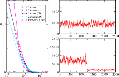
Figure 1: (color online) We performed some numerical simulations of the model (with $L=2500$) by preassigning both no (1 class) and one dominant set (2 classes). On the left we plot the frequency distribution of the weights in the network, for uniform and truncated Gaussian (G) choice of the distribution of $W$ (for a comparison we plot also the weights distribution of the COMTRADE data). On the right we plot the histogram of the number of drawings of each edge with no dominant set (up) and with the set $[1,1225]$ as the dominant set (below).

Based on the above limit relations and some asymptotic results, analytically proved in BCPR ; BCPRdom , we have developed a statistical test for the class $\cal D$. In particular, we can test the hypothesis of a given subset becoming the class of dominant edges during the evolution of the network. Similarly, it is possibile to test if a particular instance of a given network has a weight distribution that already evolved into its stationary state or not.

We assume as a null hypothesis that the “dominant set” ${\cal D}$ coincides with a certain subset of edges ${\cal D}^{*}$ with $\mbox{card}({\cal D}^{*})\geq 2$ and consider a certain level $(1-\alpha)$ (typically $\alpha=5\%,10\%$). Then we fix $\ell^{*}\in{\cal D^{*}}$ and compare the quantity (defined in the sequel)

$$\frac{|C^{*}_{u\ell^{*}}|}{\sqrt{U_{u\ell^{*}}}}$$ (8)

with the quantile $q_{\alpha}$ of the standard normal distribution ${\cal N}(0,1)$ of order $(1-\alpha/2)$ (that is $q_{\alpha}$ is the number such that ${\cal N}(0,1)(q_{\alpha},+\infty)=\frac{\alpha}{2}$ and $q_{\alpha}=1.96$ for $\alpha=5\%$ and $q_{\alpha}=1.645$ for $\alpha=10\%$). If the computed quantity is greater than $q_{\alpha}$, then we reject the null hypothesis at the (approximate) level $(1-\alpha)$; otherwise we can not reject it. The random variable $U_{u\ell^{*}}$ is defined as

$$U_{u\ell^{*}}\!=\!{\textstyle{\!\overline{X}_{u\ell^{*}}\bigl{\{}(1-\overline{X}_{u\ell^{*}})^{2}\widehat{\sigma}_{u\ell^{*}}^{2}+\overline{X}_{u\ell^{*}}\sum_{\ell\in{\cal D}^{*},\ell\neq\ell^{*}}\overline{X}_{u\ell}\,\widehat{\sigma}_{u\ell}^{2}\!\bigr{\}}\over(\widehat{\mu}^{*}_{u})^{2}\,\bigl{(}\sum_{\ell\in{\cal D}^{*}}\overline{X}_{u\ell}\bigr{)}^{4}}}$$ (9)

where $\overline{X}_{u\ell}=\sum_{n=1}^{u}X_{n\ell}/u$ and $\widehat{\mu}^{*}_{u}$ is an estimate of the mean value $\mu^{*}$ and $\widehat{\sigma}_{u\ell}^{2}$ is an estimate of the variance $\sigma_{\ell}^{2}$, i.e.

$$\begin{split}&\widehat{\mu}^{*}_{u}={\textstyle{1\over\text{card}({\cal D}^{*})}}\sum_{\ell\in{\cal D}^{*}}\left({\textstyle{\sum_{n=1}^{u}W_{n\ell}X_{n\ell}\over\sum_{n=1}^{u}X_{n\ell}}}\right),\\ &\widehat{\sigma}_{u\ell}^{2}={\textstyle{\sum_{n=1}^{u}W_{n\ell}^{2}X_{n\ell}\over\sum_{n=1}^{u}X_{n\ell}}}-\left({\textstyle{\sum_{n=1}^{u}W_{n\ell}X_{n\ell}\over\sum_{n=1}^{u}X_{n\ell}}}\right)^{2}\,.\end{split}$$ (10)

Further the random variable $C^{*}_{u\ell^{*}}$ is defined as

$$C_{u\ell^{*}}^{*}=\sqrt{u}(\overline{X}_{u\ell^{*}}^{*}-Z_{u\ell^{*}}^{*})\,,$$ (11)

where

$$\begin{split}&Z_{u\ell^{*}}^{*}={\textstyle{1+\sum_{n=1}^{u}W_{n\ell^{*}}X_{n\ell^{*}}\over\mbox{card}({\cal D}^{*})+\sum_{\ell\in{\cal D}^{*}}\sum_{n=1}^{u}W_{n\ell}X_{n\ell}}},\\ &{\overline{X}}_{u\ell^{*}}^{*}={\textstyle{\sum_{n=1}^{u}X_{n\ell^{*}}\over 1+\sum_{\ell\in{\cal D}^{*}}\sum_{n=1}^{u}X_{n\ell}}}\,.\end{split}$$ (12)

Simulations have shown that, if we perform the above test taking ${\cal D}^{*}$ exactly equal to the preassigned dominant set, then the percentage of indexes $\ell^{*}$ for which the test gives the rejection of the hypothesis is very low ($=2.28\%$ for $\alpha=10\%$ and $0.82\%$ for $\alpha=5\%$). From now on we will call this percentage the “rejection percentage”. If we consider a different ${\cal D}^{*}$ with the same cardinality of the real dominant set, the rejection percentage increases (even if we change a single element): the more ${\cal D}^{*}$ and the real dominat set are different, the higher the rejection percentage is (we got values up to $93\%$ for $\alpha=10\%$ and $85\%$ for $\alpha=5\%$). However, we observed that the power of this test decreases with the decreasing of the cardinality of ${\cal D}^{*}$. For instance, it is not able to reject the null hypothesis when ${\cal D}^{*}$ is strictly contained in the real dominant set. As a solution to this problem, we add to the previous test another statistical test obtained by replacing the random variable $U_{u\ell^{*}}$ by

$${\textstyle{\!\overline{X}_{u\ell^{*}}\!\bigl{\{}(1-\overline{X}_{u\ell^{*}})^{2}\!\widehat{\sigma}_{u\ell^{*}}^{2}\!+\!\overline{X}_{u\ell^{*}}\sum_{\ell\in{\cal D}^{*},\ell\neq\ell^{*}}\!\overline{X}_{u\ell}\widehat{\sigma}_{u\ell}^{2}\!\bigr{\}}\!\bigl{(}\!\sum_{\ell\in{\cal D}^{*}}\!\overline{X}_{u\ell}\!\bigr{)}^{2}\!\over(\widehat{\mu}^{*}_{u})^{2}}}.$$ (13)

This second test works very well for ${\cal D}^{*}$ with small cardinality (the rejection percentage goes from $80\%$ to $100\%$.)

In sum, based on these two statistical tests, we have introduced a statistical procedure to study the dominant set of a network and predict if a certain edge distribution will disappear in the steady state of the graph evolution or not.

As an application and a test, we consider the international trade network (ITN), also known in complex network literature as the world-trade web SB . ITN is defined as the network of import-export relationships between world countries in a given period (usually a year). Many efforts have been devoted to analyze the structure and the dynamics of the ITN from an empirical and theoretical modeling perspective (see, for instance, GL-2004 ; HMR ; BMSKM-2008 ; FRS-2009 ; RS ; GCC ; GL-2005 ; H . However, existing contributions are not able to rigorously explain the evidence that there exists a “club of a few rich countries” BMSKM-2008 that control a major share of the trade network. This issue of “rich-club” detection is particularly important also from a theoretical point of view. Rich club property (i.e. the proportion of vertices whose degree is larger than a certain value that are also connected each other) can be defined in a proper way only for sparse networks colizza , while no consensus exists for the case of dense networks gin as ITN. In particular, for dense networks it is particularly difficult to define a reference or null case, against which one can measure the specific features of the real system. Our model allows a natural description of this case and it also allows for a rigorous analysis of the stability of the statistical distributions. In the context of the ITN, we assume that the nodes represent the countries and the edges represent the trade between them. With regard to the weightsPNAS , there are different possibilities. The most natural choice is to define the weight of a certain edge $\ell=i,j$ in terms of the value of the flow from $i$ to $j$.

As a real case data example we consider here the data of trades between nations in the years 1948-2000 as it is possible to reconstruct from COMTRADE data COMTRADE . We computed for each year and for each couple of countries $(A,B)$ the total exports (when present) from $A$ to $B$. The ordered couple $(A,B)$ is an edge (color) while the edge weight for a certain year represents an extraction of that edge (color) where the number of added balls is the amount of dollars for the total exports for that edge in that year. For the COMTRADE data we don’t know in advance the “dominant edges” set but we can leverage from the statistical test previously defined to extract at least a core subset of it. In order to get this core subset we fixed ${\cal D}^{*}$ of size $2000$ and performed the first test for ${\cal D}^{*}$ picking up $\ell^{*}$ in descending order starting from the largest edge weight. If we then plot the number of no-rejections along the whole set of $\ell^{*}$ in ${\cal D}^{*}$, we find that for the ordered case the number of no-rejections grows linearly with constant slope close to $1$ but at a certain point starts bending (see Fig. 2). After this bending it saturates and reaches a plateau where the $\ell^{*}$ will always give a rejection. Remarkably we found an “optimal” size of ${\cal D}^{*}$ for which the difference of the rejection percentage for the ordered edges and the random case is maximal, revealing that the set of top ranking edges in that subset is the best fit for the “dominant edges” set.

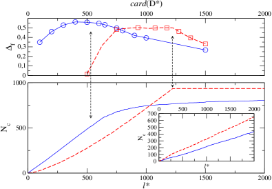
Figure 2: (color online) In the lower panel we checked the number of no-rejections for the COMTRADE data and the simulated data of an urn with colored balls in the case of uniform distributions. For both cases we considered a ${\cal D}^{*}$ of size $2000$ and ordered the edges/colors in descending order according to the edge weight/number of balls values. We then executed the test considering $\ell^{*}$ running from the highest to the lowest value and accumulating the number of no-rejections in the $y$-axis. After a constant no-rejection rate the COMTRADE data (blue line) start bending, signaling the presence of a core subset of dominant edges. The same happens for the urn with colored balls (red line) but with a much more sharp turning point, exactly in correspondence of the dominant ${\cal D}^{*}$ size of $1225$, known a priori. In the inset the same procedure has been performed for a random ${\cal D}^{*}$ for the two corresponding cases. In the upper panel, we calculated the difference between the rejection percentage for the ordered and the random case and discovered a maximum where the two curves start bending.

In summary, we present here a model of weighted-network growth based on a weighted preferential attachment principle P : the probability of picking an edge depends on the total weight of that edge (and not simply on the number of times it has been picked)KSBBHS ; ZTZH . We provide a theoretical framework, which accounts for the empirical evidence that many real networks grow in a heterogeneous way generating a subset of dominant edges that controls a major share of the total weight of the network, while the weight of other connections is negligible. Our approach is quite general and flexible since it does not require a particular probability distribution or functional form of the weights. Furthermore our model produces in a natural way dense benchmark networks that can be used as a reference or benchmark towards real dense networks. The mapping with RRU has allowed us to introduce a statistical procedure for making inference on the class of dominant links. Thanks to the above procedure, it is now possible to quantitatively test the convergence to steady state in network dynamics, a problem often encountered in assessing the significance of observations in complex networks.

Authors acknowledge support from CNR, PNR project “CRISIS Lab” and FET Open project 255987 FOC.

References

- (1) R. Albert, A.L. Barabási, Review of Modern Physics, 74 (2002), 47-97.
- (2) D. Garlaschelli, S. Battiston, M. Castri, V.D.P. Servedio, G. Caldarelli, Physica A 350, 491 (2005)
- (3) M. Kitsak, M. Riccaboni, S. Havlin, F. Pammolli, H.E. Stanley, Physical Review E, 81, 036117 (2010).
- (4) J. Tinbergen, Shaping the World Economy: Suggestions for a International Economic Policy, New York: The Twentieth Century Fund, (1962).
- (5) R. Pastor-Satorras, A. Vespignani Evolution and Structure of the Internet, Cambridge Unviersity Press (2004).
- (6) M.E.J. Newman, Networks: an introduction Oxford University Press (2010).
- (7) C. Roth, S.M. Kang, M. Batty, M. Barthélemy, PLoS ONE 6, e15923. (2011).
- (8) G. Caldarelli,Scale-Free Networks, Oxford University Press (2007).
- (9) G. Aletti, C. May, P. Secchi, Advances in Applied Probability, 41 (2009), 829-844.
- (10) P. Berti, I. Crimaldi, L. Pratelli, P. Rigo, Journal of Applied Probabilities, 48, 527-546 (2011).
- (11) P. Berti, I. Crimaldi, L. Pratelli, P. Rigo, Stochastic Processes and their Applications, 120, 1473-1491 (2010).
- (12) I. Crimaldi, International Mathemaical Forum, 23 , 1139-1156 (2009).
- (13) C. May, N. Flournoy, Annals of Statistics, 37, 1058-1078 (2009).
- (14) A. Serrano, M. Boguñá, Physical Review E, 68, 015101(R) (2003).
- (15) D. Garlaschelli, M. Loffredo, Physical Review Letters, 93, 188701 (2004).
- (16) E. Helpman, M. Melitz, Y. Rubinstein, NBER working paper series, 12927 (2007).
- (17) K. Bhattacharya, G. Mukherjee, J. Saramäki, K. Kaski, S.S. Manna, Journal of Statistical Mechanics, P02002 (2008).
- (18) G. Fagiolo, J. Reyes, S. Schiavo, Physical Review E, 79, 036115 (2009).
- (19) M. Riccaboni, S. Schiavo, New Journal of Physics, 12, 023003 (2010).
- (20) D. Garlaschelli, A. Capocci, G. Caldarelli, Nature Physics, 3 , 813-817 (2007).
- (21) D. Garlaschelli, M. Loffredo, Physica A, 355, 138-144 (2005).
-
(22)
K. Head, Gravity for beginners, (2003), available at
http://economics.ca/keith/gravity.pdf - (23) V. Colizza, A. Flammini, M. A. Serrano and A. Vespignani, Nature Physics 2, 110 - 115 (2006).
- (24) V. Zlatić, G. Bianconi, A. Díaz-Guilera, D. Garlaschelli, F. Rao, G. Caldarelli, European Physical Journal B 67, 271-275 (2009).
- (25) A. Barrat, M. Barthélemy, A. Vespignani, Physical Review Letters, 92, 228701 (2004).
- (26) United Nations Commodity Trade Statistics Database http://comtrade.un.org/.
- (27) R. Pemantle, A survey of random processes with reinforcement, Probability Surveys 4 , 1-79 (2007).
- (28) T. Kalisky, S. Sreenivasan, L.A. Braunstein, S.V. Buldyrev, S. Havlin, H.E. Stanley, Physical Review E, 73, 025103(R) (2006).
- (29) D. Zheng, S. Trimper, B. Zheng, P. Hui, Physical Review E, 67, 040102 (2003).