Co-evolution of Galaxies and Central Black Holes:
Observational Evidence on the Trigger of AGN Feedback

Abstract

A comprehensive analysis of extended emission line region (EELR) around quasars is presented. New Subaru/Suprime-Cam observation is combined with literature search, resulting in a compilation of 81 EELR measurements for type-1 and type-2 quasars with associated active galactic nucleus (AGN) and host galaxy properties. It is found that EELR phenomenon shows clear correlation with Eddington ratio, which links EELR to the constituents of the principal component 1 (PC 1), or eigenvector 1, of the AGN emission correlations. We also find that EELR is preferentially associated with gas-rich, massive blue galaxies. It supports the idea that the primary determinant of EELR creation is the gas availability and that the gas may be brought in by galaxy merger triggering the current star formation as well as AGN activity, and also gives an explanation for the fact that most luminous EELR is found around radio-loud sources with low Eddington ratio. By combining all the observations, it is suggested that EELR quasars occupy the massive blue corner of the green valley, the AGN realm, on the galaxy color - stellar mass diagram. Once a galaxy is pushed to this corner, activated AGN would create EELR by the energy injection into the interstellar gas and eventually blow it away, leading to star-formation quenching. The results presented here provide a piece of evidence for the presence of such AGN feedback process, which may be playing a leading role in the co-evolution of galaxies and central super-massive black holes.

1. Introduction

Some active galactic nuclei (AGNs) are surrounded by massive ionized nebulae extending to several tens of kiloparsec from the central engines. The first systematic study of such extended emission-line region (EELR) around quasars in combination with nuclear spectral properties was presented by Boroson & Oke (1984) and Boroson et al. (1985). They found that nearly half of their 24 objects are EELR quasars (quasars with detectable EELR, following Fu & Stockton, 2007) and that the EELR quasars have larger [O III] $\lambda$5007 equivalent width (EW), broader and bumpier Balmer lines, and weaker Fe II emission compared to non-EELR quasars. In addition, the EELR quasars are predominantly associated with steep-spectrum radio emission with extended, lobe-dominant morphology, in contrast to the non-EELR quasars associated with flat-spectrum radio emission with compact, core-dominant morphology or without strong radio emission.

The correlation between EELR phenomenon and radio emission was further confirmed by Stockton & MacKenty (1987), who obtained narrow-band [O III] line images of 47 quasars. Above the limiting luminosity of extended [O III] emission $L_{\rm E[OIII]}=5\times 10^{41}$ erg s^-1, 10 out of 26 (10/26) of their steep-spectrum radio quasars (SSRQs) have EELR, while majority of the flat-spectrum radio quasars (FSRQs) and the radio-quiet quasars (RQQs; 7/7 of the FSRQs and 13/14 of the RQQs) are non-EELR sources (Fu & Stockton, 2009). They also found a correlation between nuclear [O III] luminosity and the presence of EELR. Fu & Stockton (2007) analyzed the rest-frame ultraviolet spectra of 12 SSRQs in the Stockton & MacKenty (1987) sample and found that N V $\lambda$1240 emission is suppressed in EELR quasars, which they claimed points to lower metallicity of the broad-line region (BLR) compared to non-EELR quasars. They did not find any systematic difference in other AGN properties such as continuum luminosity and mass of super-massive black holes (SMBHs) between the EELR and non-EELR SSRQs.

On the other hand, Husemann et al. (2008) observed 20 quasars dominated by RQQs and found EELR around 8 of them. The correlation between nuclear Fe II EW, H$\beta$ line width, and EELR was confirmed in their sample too. In addition, they found a dependence of EELR on SMBH mass ($M_{\rm BH}$) and reported that $M_{\rm BH}=10^{8.5}M_{\odot}$ separates EELR quasars with larger $M_{\rm BH}$ from non-EELR quasars with smaller $M_{\rm BH}$. Searches for EELR around RQQs were also presented by Humphrey et al. (2010) and Villar-Martín et al. (2010, 2011) focusing on obscured, type-2 quasars. They found EELR around 10 out of 20 objects and claimed that luminous EELR is not necessarily associated with powerful radio sources.

Observational constraints on the emergence of EELR can possibly be a key to understand the co-evolution of galaxies and SMBHs. It is now widely accepted that the tight correlation between SMBH mass and bulge mass of their host galaxies (e.g., Magorrian et al., 1998; Häring & Rix, 2004) indicates the intimately-connected evolution of the two systems. The most compelling process of interaction between galaxies and SMBHs is the AGN feedback, in which the energy emitted by AGN regulates the mass accretion to SMBHs and drives galactic wind that can expel cold gas from and quench star formation in host galaxies. The AGN feedback could also give a solution to the two major problems in the current galaxy formation models based on the $\Lambda$ cold dark matter (CDM) theory: first is the ”overcooling” problem in which much more massive galaxies are formed in the numerical simulations than observed due to too efficient gas cooling, and second is the ”inverted color - mass - morphology relation” problem in which massive galaxies are predicted to be blue and disk-dominant rather than red and spheroid-dominant as observed (e.g., Somerville et al., 2008). However, observational evidence is still lacking on whether the AGN feedback is actually present or not and how it works if present. While measurements of galaxy evolution imprinted on the stellar-mass (luminosity) function (e.g., Bell et al., 2004; Faber et al., 2007; Brown et al., 2007, 2008) especially at its massive end (Conselice et al., 2007; Matsuoka & Kawara, 2010; Matsuoka et al., 2011a) and its integration (the extragalactic background light; e.g, Matsuoka et al., 2011b), or analyses of the nature of the AGN phenomenon (e.g., Laor, 2000; Boroson, 2002; Matsuoka et al., 2007, 2008; Vestergaard et al., 2008) can put indirect constraints on the co-evolution, EELR possibly provides more direct clues as to the interrelation between galaxies and SMBHs. The previous measurements indicate that EELR gas is largely ionized by AGN rather than stellar population (Fu & Stockton, 2009; Husemann et al., 2010; Keel et al., 2012), hence we may be witnessing the AGN feedback in action in this galaxy-wide ionization process. Indeed, Greene et al. (2011) recently showed that AGN photoionizes and kinematically disturbs the interstellar medium throughout the entire host galaxies of luminous type-2 quasars.

In this paper, new observation of EELR around five quasars at $z\sim 0.3$ is first presented. Then it is combined with the previous observations of EELR and associated AGN and host galaxy properties obtained mainly from the Sloan Digital Sky Survey (SDSS; York et al., 2000) archive. By using this compiled sample as well as the control samples of SDSS quasars and galaxies, we aim to perform a comprehensive analysis of EELR in the context of galaxy evolution. A cosmology with $H_{0}$ = 70 km s^-1 Mpc^-1, $\Omega_{\rm M}=0.3$, and $\Omega_{\rm\Lambda}=0.7$ is assumed throughout this work. Luminosity and mass are given in units of erg s^-1 and the solar mass ($M_{\odot}$) unless otherwise noted. All the presented magnitudes are on the AB system.

2. Data

2.1. New Observation

The observed quasars were selected from the SDSS Data Release 7 (DR7) quasar catalog (Schneider et al., 2010; Shen et al., 2011). The simple selection criteria were set based on redshift ($z\simeq 0.3$ in order that [O III] $\lambda$5007 falls in the narrow-band filter transmission described below) and nuclear [O III] luminosity ($L_{\rm N[OIII]}>10^{42}$ erg s^-1). Among the objects meeting the criteria, those with various SMBH mass and radio loudness and with the highest [O III] luminosity were picked up. The properties of the observed quasars are summarized in Table 1. They effectively complement the existing measurements on the AGN principal-component plane explored below.

The targets were observed with the prime-focus imaging facility Suprime-Cam (Miyazaki et al., 2002) mounted on Subaru telescope. The instrument covers a wide field-of-view of 34 $\times$ 27 arcmin² with ten 2k $\times$ 4k CCDs, with a pixel scale of 0.20 arcsec. The narrow-band NA₆₅₆ (effective wavelength $\lambda_{\rm eff}$ = 6570 Å, effective bandpass $\Delta\lambda_{\rm eff}$ = 140 Å) and the broad-band $R_{\rm c}$ ($\lambda_{\rm eff}$ = 6530 Å, $\Delta\lambda_{\rm eff}$ = 1110 Å) filters were used to trace the redshifted [O III] line and underlying continuum, respectively. The observation was carried out on 2011 May 3–4 under the open-use program S11A-028. The sky condition was sometimes non-photometric, but the measured flux of celestial objects was mostly stable within 10 % variation. The seeing was 0.8–1.1 arcsec. For each target, nine 300-sec or three 900-sec exposures in NA₆₅₆ and nine 100-sec or three 300-sec exposures in $R_{\rm c}$ were obtained, depending on the source brightness. In addition, a spectrophotometric standard star SA 104-335 was observed with the same instrument configuration as the target observation.

Table 1Targets of Subaru/Suprime-Cam observation.

	$r$-band		log $L_{\rm N[O\ III]}$	log $M_{\rm BH}$		log $L_{\rm E[O\ III]}$
Quasar	mag.	Redshift	(erg s-1)	($M_{\odot}$)	R	(erg s-1)
SDSS 091401.75$+$050750.6	17.32	0.301	42.85 $\pm$ 0.01	9.36 $\pm$ 0.10	L	42.17 $\pm$ 0.08
SDSS 095456.89$+$092955.7	17.92	0.298	42.93 $\pm$ 0.01	8.56 $\pm$ 0.08	L	$<$ 41.47
SDSS 113949.47$+$402048.5	17.52	0.314	42.97 $\pm$ 0.01	8.21 $\pm$ 0.08	Q	$<$ 41.48
SDSS 150740.92$+$445331.5	18.16	0.314	42.69 $\pm$ 0.01	7.34 $\pm$ 0.14	L	$<$ 41.53
SDSS 150752.66$+$133844.5	17.79	0.322	42.53 $\pm$ 0.01	9.67 $\pm$ 0.02	Q	41.83 $\pm$ 0.08

Note — ^aSDSS PSF magnitude. The measurement error is $<$ 0.02 mag. ^bRadio loudness. Q: radio quiet, L: radio loud.

Data reduction was performed with the Suprime-cam Deep Field Reduction (SDFRED; Ouchi et al., 2004) software in a standard manner, including bias subtraction, flat fielding, distortion correction, sky subtraction, masking bad pixels, and stacking. Photometric calibration in NA₆₅₆ was achieved by referring to the observed flux of SA 104-335, whose intrinsic magnitude was derived by convolving its spectrophotometry data (Stone, 1996) with the filter transmission function. Then the $R_{\rm c}$ images were calibrated relative to NA₆₅₆ by requiring the mean ($R_{\rm c}$ $-$ NA₆₅₆) color to be zero for galaxies detected with high signal-to-noise ratios (point sources were not used because stellar H$\alpha$ absorption could affect this calibration). The scatter of $\sim$0.05 mag was found around the mean between $R_{\rm c}$ and NA₆₅₆ magnitudes in the calibration.

The reduction process then proceeded to the continuum subtraction from the NA₆₅₆ images. For this purpose, the nuclear spectra of the quasars were retrieved from the SDSS DR7 archive (an example is shown in Figure 1). They were measured within SDSS spectroscopic fibers of 3-arcsec aperture. For each spectrum, the continuum levels beneath [O III] $\lambda$4959 and $\lambda$5007 were estimated by interpolation between continuum windows at both (shorter- and longer-wavelength) sides of the lines, and then the spectrum was decomposed into [O III] and continuum. Convolving them with the filter transmissions gives us the relative fluxes of [O III] and continuum in NA₆₅₆ ($f_{\rm NA_{656}}^{\rm[OIII]}$ and $f_{\rm NA_{656}}^{\rm cont}$) and in $R_{\rm c}$ ($f_{R_{\rm c}}^{\rm[OIII]}$ and $f_{R_{\rm c}}^{\rm cont}$) for each object. Using these measures, accurate continuum subtraction was achieved as follows. The radial profiles of all the quasar nuclei on the obtained images are consistent with the point spread functions (PSFs) derived from nearby stars, hence they are dominated by the radiation from central unresolved sources. The NA₆₅₆ and $R_{\rm c}$ images were decomposed into nuclear (${\rm NA}_{656}^{\rm nuc}$, ${R}_{\rm c}^{\rm nuc}$) and extended (${\rm NA}_{656}^{\rm ext}$, ${R}_{\rm c}^{\rm ext}$) components by the best-fit Moffat profiles, fitted within a 10-pixel (2-arcsec) aperture on top of the quasar peak positions. Then the nuclear [O III] distributions are given by

$${\rm NA}_{656}^{\rm nuc}\times\frac{f_{\rm NA_{656}}^{\rm[OIII]}}{f_{\rm NA_{656}}^{\rm[OIII]}+f_{\rm NA_{656}}^{\rm cont}},$$ (1)

while the extended [O III] distributions are

$$({\rm NA}_{656}^{\rm ext}-{R}_{\rm c}^{\rm ext})\times\frac{f_{\rm NA_{656}}^{\rm[OIII]}}{f_{\rm NA_{656}}^{\rm[OIII]}-f_{R_{\rm c}}^{\rm[OIII]}}.$$ (2)

The second term in the expression (2), which is equivalent in principle to the ratio $\Delta\lambda_{\rm eff,R_{\rm c}}$ / ($\Delta\lambda_{\rm eff,R_{\rm c}}-\Delta\lambda_{\rm eff,NA_{656}}$), corrects for the continuum oversubtraction of the first term due to the [O III] themselves contained in ${R}_{\rm c}^{\rm ext}$. Note that the expression (1), although it is most accurate, is not applicable to the extended components since the relative fluxes of [O III] and continuum are different from $f_{\rm NA_{656}}^{\rm[OIII]}$ and $f_{\rm NA_{656}}^{\rm cont}$ measured in the SDSS spectroscopic fibers. It is worth re-emphasizing that the spectral information is quite useful in the above process as an accurate cross-calibrator of the images taken in the different filters.

Figure 1.— Nuclear spectrum of SDSS 1139$+$4020 (solid line) with the arbitrary-scaled transmission functions of broad-band $R_{\rm c}$ and narrow-band NA₆₅₆ filters (dotted lines).

2.2. Data Compilation

Thanks to the massive spectroscopic observations conducted by the SDSS, nuclear properties are now known for many quasars with EELR measurements in the literature. We compile the EELR measurements of type-1 quasars from Boroson et al. (1985), Stockton & MacKenty (1987), and Husemann et al. (2008, 2010). The continuum and line luminosities given in Stockton & MacKenty (1987) are converted to the values in the cosmology adopted here. The measurements of Husemann et al. (2008) are corrected in accordance with their re-analysis (Husemann et al., in preparation). Then we cross-match the quasars with the SDSS DR7 quasar catalog (Shen et al., 2011) and obtain the nuclear properties such as continuum and line luminosity, SMBH mass, and radio characteristics based on the Faint Images of the Radio Sky at Twenty cm survey (FIRST; Becker et al., 1995). For some objects without counterparts in the SDSS catalog, the nuclear properties are taken from the above papers as well as Fu & Stockton (2007). Combined with the new observation presented in this paper, we end up with 61 type-1 quasars with EELR measurements (27 detections and 34 non-detections) and with a variety of nuclear properties. The compiled sample is listed in Table 2.2. We assign radio flag 0 to RQQs, flag 1 to flat-spectrum (radio spectral index $\alpha_{\nu}<0.5$) or core-dominant (based on the FIRST morphology; Jiang et al., 2007) radio quasars, flag 2 to steep-spectrum ($\alpha_{\nu}>0.5$) or lobe-dominant radio quasars. The SDSS quasars are separated into radio-quiet and radio-loud sources at the radio-loudness parameter $R$ = 5 (Shen et al., 2011). For simplicity the objects with radio flag 0, 1, 2 are hereafter referred to as RQQs, FSRQs, and SSRQs, respectively, since there is a well-known, strong correlation between the radio morphology and spectral index.

Table 2Nuclear properties of type-1 quasars with EELR measurements.

		log $\lambda L_{\rm\lambda 5100}$	log $M_{\rm BH}$		log $L_{\rm N[OIII]}$	log $L_{\rm E[OIII]}$
Quasar	Redshift	(erg s-1)	($M_{\odot}$)	R	(erg s-1)	(erg s-1)	Ref.
4C 15.01	0.450	45.61	9.24	2	43.58	$<$ 42.56	2
PG 0026$+$129	0.142	44.96 $\pm$ 0.11	8.98	0	42.53 $\pm$ 0.09	41.80 $\pm$ 0.14	3
PG 0050$+$124	0.061	44.31 $\pm$ 0.11	8.00	0	42.26 $\pm$ 0.09	$<$ 43.0	3
PG 0052$+$251	0.155	44.98 $\pm$ 0.10	8.55	0	42.70 $\pm$ 0.09	41.75 $\pm$ 0.13	1, 2, 3
SDSS 0057$+$1446	0.172	44.93 $\pm$ 0.01	9.38 $\pm$ 0.02	0	42.23 $\pm$ 0.03	$<$ 43.0	3
HE 0132$-$0441	0.154	44.69 $\pm$ 0.10	7.73	0	42.15 $\pm$ 0.16	$<$ 43.0	3
NAB 0137$-$01	0.334	45.17 $\pm$ 0.01	9.01 $\pm$ 0.02	0	42.62 $\pm$ 0.02	$<$ 41.53	2
SDSS 0155$-$0857	0.165	44.43 $\pm$ 0.02	8.82 $\pm$ 0.04	0	42.15 $\pm$ 0.02	41.43 $\pm$ 0.19	3
HE 0157$-$0406	0.218	44.72 $\pm$ 0.09	8.52	0	42.09 $\pm$ 0.10	$<$ 43.0	3
Mrk 1014	0.163	44.78 $\pm$ 0.01	8.06 $\pm$ 0.05	1	42.74 $\pm$ 0.02	42.22 $\pm$ 0.14	2, 3
OI 287	0.444	45.08 $\pm$ 0.01	9.09 $\pm$ 0.21	2	43.51 $\pm$ 0.01	$<$ 42.47	2
SDSS 0836$+$4426	0.254	45.29 $\pm$ 0.01	8.73 $\pm$ 0.06	0	43.28 $\pm$ 0.01	43.08 $\pm$ 0.09	3
SDSS 0914$+$0507	0.301	44.84 $\pm$ 0.01	9.36 $\pm$ 0.10	2	42.85 $\pm$ 0.01	42.30 $\pm$ 0.08	5
SDSS 0948$+$4335	0.226	44.76 $\pm$ 0.01	8.43 $\pm$ 0.03	0	42.44 $\pm$ 0.01	$<$ 43.0	3
SDSS 0954$+$0929	0.298	44.54 $\pm$ 0.01	8.56 $\pm$ 0.08	2	42.93 $\pm$ 0.01	$<$ 41.60	5
Ton 28	0.329	45.44 $\pm$ 0.01	8.03 $\pm$ 0.43	0	42.42 $\pm$ 0.02	$<$ 42.34	2
4C 13.41	0.241	45.41 $\pm$ 0.01	9.54 $\pm$ 0.05	2	42.40 $\pm$ 0.02	$<$ 41.41	2
HE 1029$-$1401	0.086	44.97 $\pm$ 0.05	8.70	0	$\cdots$	41.78 $\pm$ 0.12	4
PG 1049$-$005	0.359	45.59 $\pm$ 0.01	9.17 $\pm$ 0.03	0	43.47 $\pm$ 0.01	$<$ 42.31	2
4C 61.20	0.421	45.26 $\pm$ 0.01	9.10 $\pm$ 0.09	1	43.34 $\pm$ 0.01	$<$ 42.55	2
4C 10.30	0.422	44.78 $\pm$ 0.01	9.33 $\pm$ 0.05	2	42.75 $\pm$ 0.01	$<$ 41.62	2
3C 249.1	0.313	45.42	8.96	2	43.46	42.85 $\pm$ 0.02	1, 2
SDSS 1131$+$2632	0.244	44.56 $\pm$ 0.02	9.08 $\pm$ 0.04	0	42.81 $\pm$ 0.01	42.11 $\pm$ 0.14	3
SDSS 1139$+$4020	0.314	44.63 $\pm$ 0.01	8.21 $\pm$ 0.08	0	42.97 $\pm$ 0.01	$<$ 41.61	5
4C 49.22	0.334	44.70 $\pm$ 0.01	8.50 $\pm$ 0.01	1	42.45 $\pm$ 0.01	$<$ 41.81	2
GQ Comae	0.165	44.15 $\pm$ 0.01	8.36 $\pm$ 0.03	0	42.58 $\pm$ 0.01	40.19 $\pm$ 0.30	1, 2
PKS 1217$+$023	0.240	45.13 $\pm$ 0.01	8.87 $\pm$ 0.08	2	42.78 $\pm$ 0.01	41.82 $\pm$ 0.16	2, 3
4C 25.40	0.268	44.73 $\pm$ 0.01	8.86 $\pm$ 0.03	2	42.66 $\pm$ 0.01	42.61 $\pm$ 0.02	2
3C 273	0.158	46.04 $\pm$ 0.09	9.06	1	42.87 $\pm$ 0.10	$<$ 41.73	1, 2, 3
SDSS 1230$+$6621	0.184	44.53 $\pm$ 0.01	8.26 $\pm$ 0.03	0	42.66 $\pm$ 0.01	41.90 $\pm$ 0.15	3
HE 1228$+$0131	0.117	44.95 $\pm$ 0.09	8.29	0	42.23 $\pm$ 0.11	$<$ 43.0	3
SDSS 1230$+$1100	0.236	44.73 $\pm$ 0.01	8.60 $\pm$ 0.05	0	42.64 $\pm$ 0.01	$<$ 43.0	3
PG 1307$+$085	0.154	44.80 $\pm$ 0.01	8.59 $\pm$ 0.05	0	42.69 $\pm$ 0.01	$<$ 41.06	2
B2 1425$+$267	0.364	45.14 $\pm$ 0.02	9.66 $\pm$ 0.03	2	42.99 $\pm$ 0.01	42.37 $\pm$ 0.04	1, 2
PG 1427$+$480	0.221	44.62 $\pm$ 0.01	7.95 $\pm$ 0.03	0	42.52 $\pm$ 0.01	$<$ 43.0	3
SDSS 1444$+$0633	0.208	44.48 $\pm$ 0.01	8.33 $\pm$ 0.03	0	42.44 $\pm$ 0.01	$<$ 43.0	3
HE 1453$-$0303	0.206	45.31 $\pm$ 0.12	8.59	0	42.54 $\pm$ 0.12	$<$ 43.0	3
SDSS 1507$+$4453	0.314	44.39 $\pm$ 0.01	7.34 $\pm$ 0.14	1	42.69 $\pm$ 0.01	$<$ 41.66	5
SDSS 1507$+$1338	0.322	44.79 $\pm$ 0.01	9.67 $\pm$ 0.02	0	42.53 $\pm$ 0.01	41.96 $\pm$ 0.08	5
4C 37.43	0.371	45.21 $\pm$ 0.01	9.37 $\pm$ 0.11	2	43.18 $\pm$ 0.01	43.02 $\pm$ 0.01	1,2
PG 1519$+$226	0.136	44.40 $\pm$ 0.01	7.90 $\pm$ 0.07	0	41.34 $\pm$ 0.09	$<$ 43.0	1
OR 241	0.254	44.86 $\pm$ 0.01	8.44 $\pm$ 0.05	1	42.39 $\pm$ 0.01	$<$ 41.85	2
3CR 323.1	0.265	45.20 $\pm$ 0.01	9.07 $\pm$ 0.03	2	42.99 $\pm$ 0.01	42.35 $\pm$ 0.13	1, 2, 3
4C 11.50	0.436	44.99 $\pm$ 0.01	8.87 $\pm$ 0.08	2	43.23 $\pm$ 0.01	42.68 $\pm$ 0.03	2
Ton 256	0.131	44.51 $\pm$ 0.01	7.99 $\pm$ 0.02	1	43.00 $\pm$ 0.01	42.80 $\pm$ 0.12	1, 3
SDSS 1655$+$2146	0.154	44.67 $\pm$ 0.01	8.28 $\pm$ 0.04	0	43.03 $\pm$ 0.01	43.03 $\pm$ 0.09	3
PG 1700$+$518	0.292	45.43 $\pm$ 0.09	8.98	0	42.63 $\pm$ 0.10	41.81 $\pm$ 0.18	2, 3
3CR 351	0.372	45.79 $\pm$ 0.01	9.81 $\pm$ 0.04	2	43.50 $\pm$ 0.01	$<$ 42.37	2
II Zw 136	0.061	44.40 $\pm$ 0.10	8.27	0	41.95 $\pm$ 0.09	40.90 $\pm$ 0.32	1, 3
PKS 2135$-$147	0.200	44.97	9.15	2	43.16	41.85 $\pm$ 0.04	2
HE 2152$-$0936	0.192	45.59 $\pm$ 0.10	8.76	0	42.17 $\pm$ 0.11	$<$ 43.0	3
HE 2158$-$0107	0.213	44.89 $\pm$ 0.11	8.60	0	42.59 $\pm$ 0.09	42.32 $\pm$ 0.13	3
HE 2158$+$0115	0.160	44.21 $\pm$ 0.10	7.94	0	42.01 $\pm$ 0.09	$<$ 43.0	3
4C 31.63	0.298	45.99	8.54	1	42.92	$<$ 42.08	1, 2
PG 2214$+$139	0.067	44.44 $\pm$ 0.11	8.64	0	41.81 $\pm$ 0.10	$<$ 43.0	3
PG 2233$+$134	0.326	45.19 $\pm$ 0.01	8.57 $\pm$ 0.31	0	42.50 $\pm$ 0.07	$<$ 40.58	2
PKS 2251$+$113	0.325	45.07	9.15	2	42.98	42.51 $\pm$ 0.04	1, 2
HE 2307$-$0254	0.221	44.89 $\pm$ 0.10	8.39	0	42.00 $\pm$ 0.11	$<$ 43.0	3
4C 09.72	0.433	45.17	9.30	2	42.80	$<$ 42.71	2
PKS 2349$-$014	0.174	44.77 $\pm$ 0.02	8.81 $\pm$ 0.03	2	42.45 $\pm$ 0.01	42.11 $\pm$ 0.11	3
HE 2353$-$0420	0.229	44.42 $\pm$ 0.10	8.12	0	42.58 $\pm$ 0.09	42.47 $\pm$ 0.12	3

References. — (1) Boroson et al. 1985; (2) Stockton & MacKenty 1987; (3) Husemann et al. 2008 (including the re-analyzed data given in Husemann et al. in prep.); (4) Husemann et al. 2010; (5) this work.

We also collect the EELR measurements of 20 type-2 quasars (10 detections and 10 non-detections) presented by Humphrey et al. (2010) and Villar-Martín et al. (2010, 2011). Since they were selected from the SDSS type-2 quasars identified by Zakamska et al. (2003), luminosity and EW of emission lines arising from the narrow-line region (NLR) as well as optical $ugriz$ magnitudes of the host galaxies are available in the archive. We derive the rest-frame $g-i$ color and stellar mass of the host galaxies from the SDSS model magnitudes and spectroscopic redshifts, using a $k$-correction code developed by Blanton & Roweis (2007). The contributions of relatively strong [O II] $\lambda$3727 and [O III] $\lambda$4959, $\lambda$5007 lines from quasars are removed before the calculation by subtracting $\Delta m_{X}$ = $-2.5$ log (1 + $f_{X,Y}$ [EW_Y/$w_{X}$]) from $X$ ($u$, $g$, $r$, $i$, or $z$)-band magnitude if the line $Y$ is included in the band, where $f_{X,Y}$ is the filter transmission at the line $Y$ relative to the band average and $w_{X}$ is the band width. We summarize the derived properties of the type-2 quasars in Table 2.2. All but two sources, SDSS 1228$+$0050 and SDSS 1625$+$3106, are radio quiet (SDSS 1625$+$3106 is in the transition range of radio-quiet and radio-loud objects; Villar-Martín et al., 2011). In addition, we use all the type-2 quasars in Zakamska et al. (2003) and $\sim$60,000 galaxies extracted from the SDSS galaxy sample at $z$ = 0.3 – 0.6, the redshift range of the main sample (the type-2 quasars in Table 2.2), as control objects. Their rest-frame color and stellar mass are calculated in the same way as for the objects in the main sample.

Table 3Nuclear and host galaxy properties of type-2 quasars with EELR measurements.

		log $L_{\rm N[OIII]}$	Rest-frame	Stellar mass
Quasar	Redshift	(erg s-1)	$g-i$ (mag)	log $M_{\star}(M_{\odot})$	EELR	Ref.
SDSS 0025$-$1040	0.303	42.32	0.75	11.0	$+1$	3
SDSS 0123$+$0044	0.399	42.72	1.14	10.9	$+1$	2
SDSS 0217$-$0013	0.344	42.34	0.93	11.1	$+1$	3
SDSS 0234$-$0745	0.310	42.36	0.91	10.5	$-1$	3
SDSS 0840$+$3838	0.313	42.21	1.13	11.4	$+1$	1
SDSS 0849$+$0150	0.376	41.65	1.01	10.9	$-1$	3
SDSS 0920$+$4531	0.402	42.63	0.91	11.1	$-1$	1
SDSS 0955$+$0346	0.421	42.19	1.24	11.2	$+1$	3
SDSS 1153$+$0326	0.575	43.20	0.62	11.2	$+1$	3
SDSS 1228$+$0050	0.575	42.87	0.85	11.0	$-1$	3
SDSS 1307$-$0214	0.425	42.51	1.09	11.4	$+1$	3
SDSS 1337$-$0128	0.329	42.31	0.90	11.3	$+1$	3
SDSS 1407$+$0217	0.309	42.49	0.86	10.5	$-1$	3
SDSS 1413$-$0142	0.380	42.84	1.18	11.0	$-1$	3
SDSS 1546$-$0005	0.383	41.77	1.18	11.0	$-1$	3
SDSS 1550$+$3950	0.347	43.05	0.60	11.3	$+1$	1
SDSS 1625$+$3106	0.379	42.60	1.35	11.1	$-1$	1
SDSS 1726$+$6021	0.333	42.16	0.96	10.5	$-1$	1
SDSS 1739$+$5442	0.384	42.01	1.24	11.1	$-1$	1
SDSS 2358$-$0009	0.402	42.91	0.88	11.1	$+1$	3

References. — (1) Humphrey et al. 2010; (2) Villar-Martín et al. 2010; (3) Villar-Martín et al. 2011.

While the above samples of type-1 and type-2 objects are used below to probe the different aspects of quasars, we should keep in mind that the two populations can be intrinsically different. Elitzur (2012) clarified this point by demonstrating that the two types of AGNs are drawn preferentially from the distribution of dust-torus covering factors. Since type-2 AGNs have dustier environments around them than type-1 counterparts, their host galaxies might tend to have higher star-formation rates since (i) the presence of ample dust indicates active star formation producing them; and (ii) the negative feedback (suppression of star formation) by the AGN radiation might be weaker due to the dust obscuration.

3. Emergence of EELR

3.1. Notes on New Sample

The Suprime-Cam [O III] line images of the newly observed quasars are presented in Figure 2. To aid visual inspection, the grayscale consistently represents linear flux levels between zero and quasar peak values while the white crosses indicate the PSF sizes (twice the full-widths at half-maximum [FWHMs]). The most spectacular feature is found around SDSS 1507$+$1338. The emission feature, extending across $\sim$50 kpc along the NE – SW direction, is reminiscent of the ionization cones created by AGN radiation. SDSS 0914$+$0507 has apparently extended emission too, with a knot at $\sim$35 kpc away from the center in the NW direction. On the other hand, the radial profiles of SDSS 0954$+$0929, SDSS 1139$+$4020, and SDSS 1507$+$4453 are consistent with the PSFs and show no signs of EELR. We measure the EELR luminosity in an annulus of inner radius 10 kpc and outer radius 30 kpc. The wing components of the nuclear radiations are estimated from the PSFs and subtracted. The incomplete transmission of the [O III] lines through the NA₆₅₆ filter is also corrected using the filter transmission function. We include the uncertainties in the continuum subtraction and in the correction for the wing contribution of the nuclear radiation, background sky noise, and the possible flux variation assumed to be 10 % due to the non-photometric sky condition, in the error budget of the derived luminosity. The results are listed in the last column of Table 1. The above measurements support our visual inspection finding detectable EELR only in SDSS 0914$+$0507 and SDSS 1507$+$1338. The nuclear [O III] luminosity ($L_{\rm N[O\ III]}$) is also measured within a 3-arcsec aperture, and found to agree with the SDSS spectroscopic measurements within $\Delta{\rm log}L_{\rm N[O\ III]}=\pm 0.1$.

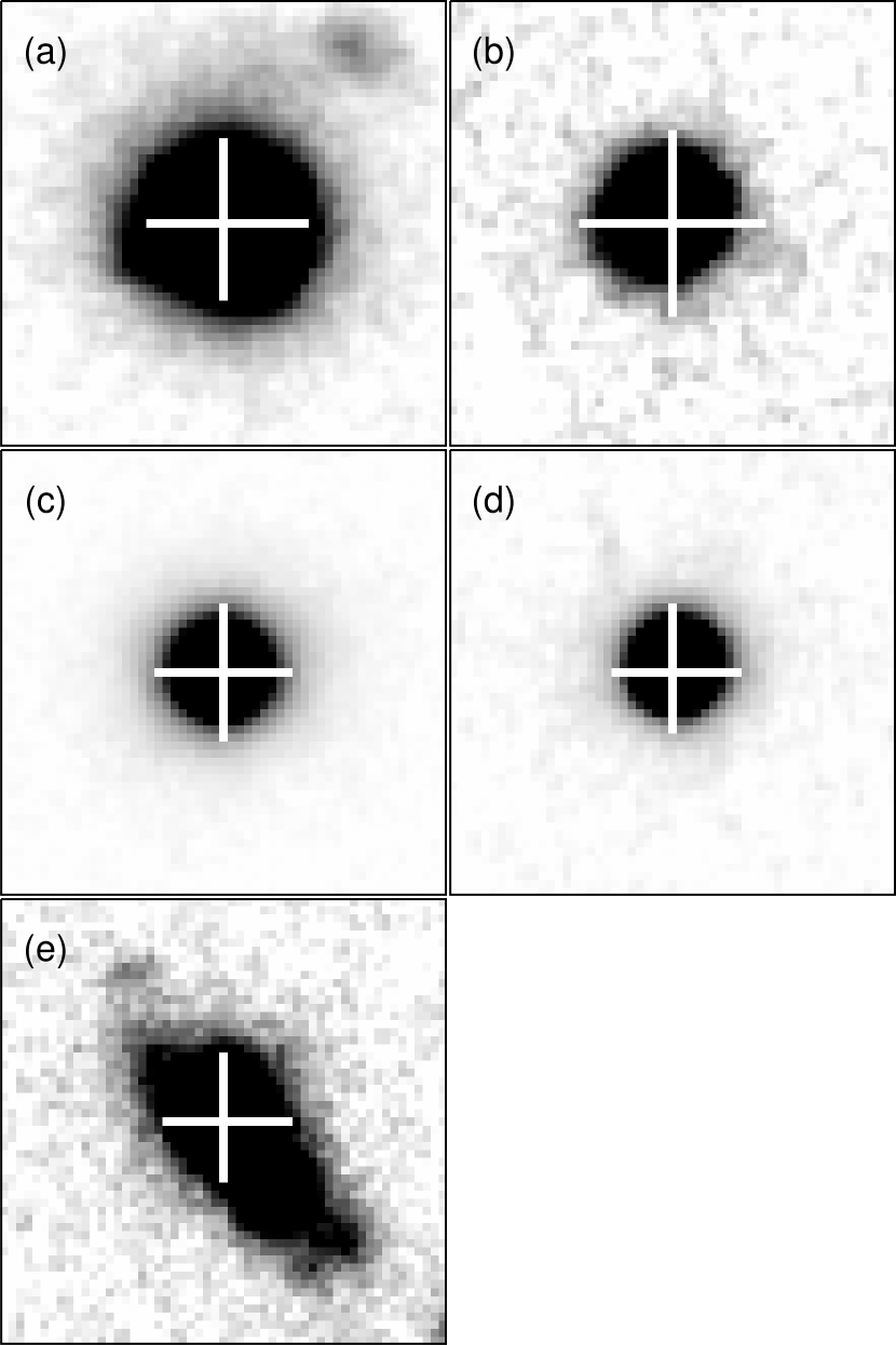
Figure 2.— Suprime-Cam [O III] line images of (a) SDSS 0914$+$0507, (b) SDSS 0954$+$0929, (c) SDSS 1139$+$4020, (d) SDSS 1507$+$4453, and (e) SDSS 1507$+$1338. The grayscale represents linear flux levels between zero and the quasar peak values, while the white crosses indicate twice the FWHMs of the PSFs. The physical scale of the panels is 50 kpc on a side. North is up, east to the left.

3.2. Link to AGN

As described in Section 1, the presence of EELR correlates with some AGN properties. Quasars with larger [O III] EW, broader and bumpier Balmer lines, fainter Fe II, and SSRQ-like radio emission have higher possibility of accompanying EELR around them. The correlation is fairly strong, as Fu & Stockton (2009) showed that if certain quasars are pre-selected based on their radio and nuclear [O III] emissions, $\sim$50 % of them would turn out to have EELR as opposed to $\sim$20 % with no a priori assumption. Note that the above emissions arise from the different parts of AGN; broad Balmer lines and the Fe II lines from parsec-scale BLR, the [O III] lines from kiloparsec-scale NLR, and radio and EELR emissions from more extended, galaxy-wide scales. The correlation among them except for EELR has been well known since the seminal work by Boroson & Green (1992). With the principal component analysis technique, they showed that most of the variance in AGN spectral properties are contained in two sets of correlations. A strong anti-correlation between the measures of [O III] and Fe II is the principal component 1 (PC 1), or eigenvector 1, with which Balmer line profile is also associated. The general consensus is that PC 1 is driven mainly by Eddington ratio (e.g., Boroson, 2002; Sameshima et al., 2011). In Figure 3 we plot H$\beta$ line width versus the relative Fe II strength $R_{\rm FeII}$ $\equiv$ EW(Fe II)/EW(H$\beta$) of the SDSS quasars in Shen et al. (2011). The both measures constitute the four-dimensional eigenvector 1 (4DE1; other measures are the soft X-ray photon index and C IV $\lambda$1549 line profile) space proposed by Sulentic et al. (2000). The anti-correlation between them is evident in Figure 3, which forms a sequence of Eddington ratio. The data scatter reflects the orientation effects as well as the intrinsic variety of quasars, since one would observe larger line FWHM and $R_{\rm FeII}$ (Fe II is emitted from the outermost part of BLR; e.g., Matsuoka et al., 2008) as the viewing angle relative to the dust-torus plane decreases. On the other hand, PC 2 links optical luminosity and He II $\lambda$4686 line emission. Its physical origin is thought to be mass-accretion rate to SMBHs because of its strong correlation with optical luminosity. Therefore one would expect that the ratio of PC 1 and PC 2 is proportional to SMBH mass, which was actually proved by Boroson (2002). Furthermore, Laor (2000) found that the radio loudness is strongly related to SMBH mass as radio-loud/radio-quiet quasars are associated with most/least massive SMBHs. The above arguments suggest that most of the AGN properties can be understood on the PC 1 - PC 2 plane.

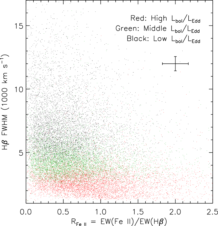
Figure 3.— H$\beta$ line width (FWHM) versus the relative Fe II strength $R_{\rm FeII}$ = EW(Fe II)/EW(H$\beta$) of the SDSS quasars. The red, green, and black dots represent the objects with high ($-0.8<$ log [$L_{\rm bol}$/$L_{\rm Edd}$]), middle ($-1.2<$ log [$L_{\rm bol}$/$L_{\rm Edd}$] $<-0.8$), and low (log [$L_{\rm bol}$/$L_{\rm Edd}$] $<-1.8$) values of Eddington ratio, respectively. The typical error of each data point is indicated at the top-right corner.

We plot Eddington ratio and continuum luminosity of the compiled type-1 sample, as well as the whole SDSS quasars in the Shen et al. (2011) catalog, in Figure 4. First of all, we remark that the objects with EELR measurements cover the distribution of the whole SDSS quasars fairly uniformly on this plane. It was not anticipated since the existing EELR observations are subject to strong selection biases individually. We see the clear separation of radio-quiet and radio-loud sources as pointed out by Laor (2000), the latter being associated with most massive SMBHs. In addition, SSRQs are observed to have higher values of Eddington ratio or SMBH mass than FSRQs. We also find some correlations containing EELR. They are shown more clearly in Figure 5 where the fraction of EELR detection is plotted as a function of the nuclear properties. The EELR fraction is strongly anti-correlated with Eddington ratio, and its weak correlation with SMBH mass may also be present. The former relation is most likely the underlying basis of the correlation between EELR and PC 1. While no clear trend is found with respect to radio emission, we do find that EELR luminosity is systematically higher in SSRQs than in the rest of the sample; the mean luminosity is $L_{\rm E[OIII]}$ = $10^{42.4}$ and $10^{41.9}$ erg s^-1 for the SSRQs and RQQs, respectively. The difference would be even larger when we consider the fact that the EELR luminosity of most SSRQs measured by Stockton & MacKenty (1987) is underestimated since the emission in a central 10-kpc aperture is excluded. It explains why the EELR fraction around SSRQs is much higher than those around the other populations in the pioneering work of Stockton & MacKenty (1987).

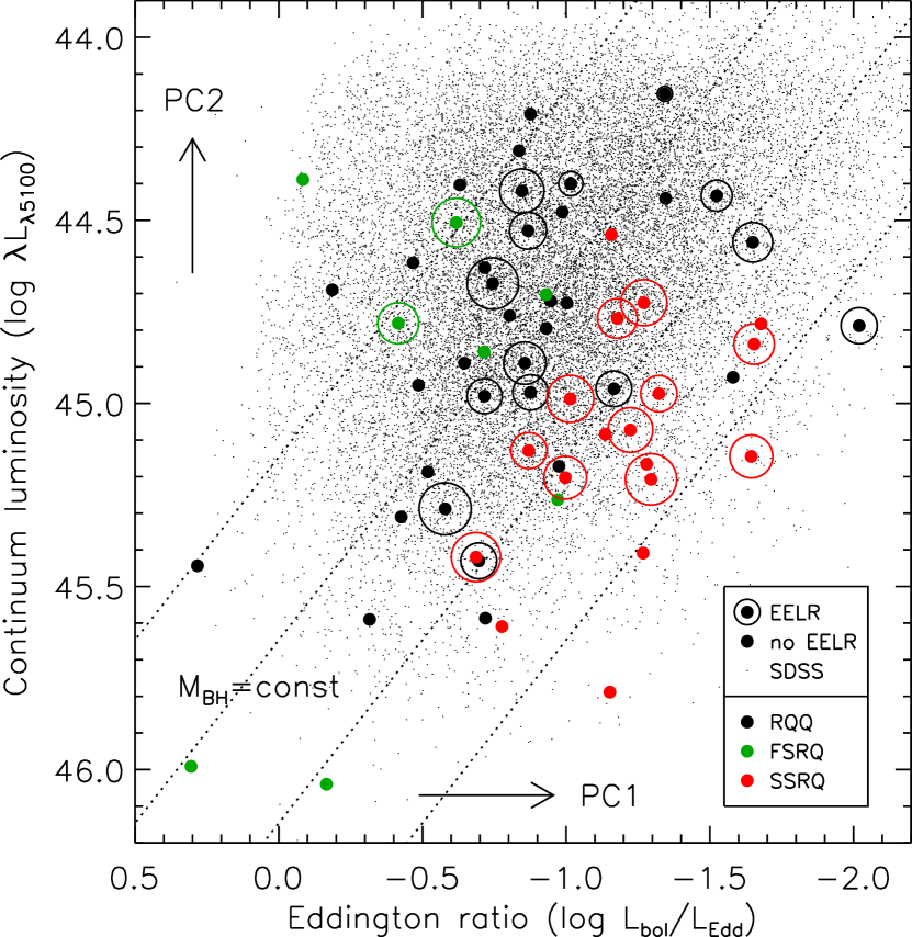
Figure 4.— Eddington ratio versus continuum luminosity of the compiled type-1 sample (filled circles) and the whole SDSS quasars (dots). RQQs, FSRQs, and SSRQs in the compiled sample are represented by black, green, and red colors, respectively. The quasars with detectable EELR are marked with the larger circles whose sizes are proportional to log $L_{\rm E[OIII]}$. PC 1 and PC 2 increase along the horizontal and vertical axes on this plane, while SMBH mass increases from the top-left to the bottom-right corner. The lines of constant SMBH mass, log $M_{\rm BH}$ = 8.0, 8.5, 9.0, 9.5, are shown by the dotted lines.

Figure 5.— Fraction of EELR detection as a function of Eddington ratio (panel a), SMBH mass (b), continuum luminosity (c), and radio-emission property (d). The fractions are calculated in the bins represented by the horizontal bars. The number of objects in each bin is also indicated.

One of the highest dependency of EELR is found on nuclear [O III] luminosity, $L_{\rm N[OIII]}$. In Figure 6 we show Eddington ratio versus $L_{\rm N[OIII]}$ of the same samples. It is clearly seen that the quasars with EELR measurements are biased to high $L_{\rm N[OIII]}$ compared to the whole SDSS quasars. Here we find that low-$L_{\rm N[OIII]}$ quasars tend to lack EELR: only 3 out of 20 objects with $L_{\rm N[OIII]}<10^{42.5}$ erg s^-1 have detectable, faint EELR, while the EELR fraction is $>$ 50 % at the higher $L_{\rm N[OIII]}$. This trend was reported previously for smaller samples (e.g., Stockton & MacKenty, 1987). Figure 6 also tells us that $L_{\rm N[OIII]}$ does not strongly correlate with Eddington ratio, although it correlates with PC 1 (Boroson & Green, 1992). No clear correlation between the two measures indicates that PC 1 is not solely driven by Eddington ratio – there should be another physical mechanism(s) that links nuclear [O III] luminosity with other PC 1 constituents.

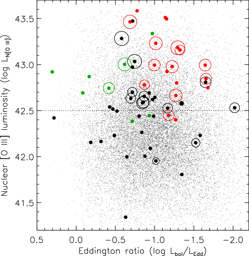
Figure 6.— Eddington ratio versus nuclear [O III] line luminosity of the compiled type-1 sample and the whole SDSS quasars. The symbols are as in Figure 4. The dotted line represents $L_{\rm N[OIII]}$ = $10^{42.5}$ erg s^-1.

What can we learn from these correlations? While the clear anti-correlation between EELR and Eddington ratio is observed, it does not seem to reflect their direct relationship through the AGN radiation since (i) the EELR fraction is highest for the AGNs with most inefficient gas accretion to SMBHs; (ii) nuclear [O III] luminosity produced similarly by the AGN radiation shows no clear correlation with Eddington ratio; (iii) a positive correlation between the EELR fraction and continuum luminosity is not observed. Therefore it is more reasonable to consider the presence of an independent mechanism that leads to the high/low EELR fraction and low/high Eddington ratio at the same time. The dependence of EELR on radio emission and (possibly) SMBH mass may also be related to this hidden mechanism. We will come back to this issue further below. The lack of simple relation between EELR and continuum luminosity (accretion rate) was also reported by Fu & Stockton (2009), who suggested that the correlation between nuclear and extended [O III] emissions, which is also evident in our larger sample, may be the sequence of the available gas amount rather than AGN emission characteristics. The hypothesis that the gas availability is the primary determinant of EELR creation is supported by the probe of host galaxies in the following section.

3.3. Link to Host Galaxies

If EELR represents a certain stage of galaxy evolution, as the AGN feedback scenario implies, their presence may be related to stellar-population properties of host galaxies. Here an investigation of such a relation is presented for the first time, thanks to the recent measurements of EELR around SDSS type-2 quasars at $z$ = 0.3 – 0.6 (Humphrey et al., 2010; Villar-Martín et al., 2010, 2011). In Figure 7, we plot stellar mass versus rest-frame $g-i$ color of the type-2 quasars as well as the control samples defined in Section 2.2. Most SDSS galaxies at these relatively high redshifts are luminous red galaxies (LRGs), forming a clump at the massive red end on this color - stellar mass diagram (we could see the red sequence rather than a clump if the SDSS observations were deep enough to detect fainter galaxies). The type-2 quasars are bluer than the LRGs (see also, Zakamska et al., 2003) but are redder than star-forming galaxies which form the ”blue cloud” around $g-i\sim 0.6$ in the local universe (e.g., Gavazzi et al., 2010). It is consistent with the result of Schawinski et al. (2010) who found that local AGNs reside in the ”green valley” between the blue cloud and the red sequence on the color - stellar mass diagram. Interestingly, we find that the EELR quasars are associated with bluer and more massive galaxies compared to the non-EELR counterparts. In order to show this trend more clearly, we define a ’massive-blue’-ness indicator, $\mathcal{I}_{\rm mb}$ $\equiv$ log M_⋆ $-$ ($g-i$), which increases diagonally toward the bottom-right corner of Figure 7 as shown by the arrow. The number distribution of the type-2 quasars with EELR measurements as a function of $\mathcal{I}_{\rm mb}$ is plotted in Figure 8. It shows a clear, monotonic increase in the fraction of EELR quasars as $\mathcal{I}_{\rm mb}$ increases: only 1/8 of the lowest-$\mathcal{I}_{\rm mb}$ quasars has EELR, while the fraction rises to 7/8 in the highest-$\mathcal{I}_{\rm mb}$ counterparts.

Figure 7.— Stellar mass versus rest-frame $g-i$ color of the galaxies hosting type-2 quasars with EELR measurements (green circles). The objects with detectable EELR are marked with the larger circles. The type-2 quasars of Zakamska et al. (2003) at $z$ = 0.3 – 0.6 are represented by the black circles, while the distribution of $\sim$60,000 SDSS galaxies in the same redshift range is shown by the contours (the contour levels are logarithmic). The arrow represents the ’massive-blue’-ness indicator $\mathcal{I}_{\rm mb}$ used in Figure 8.

Figure 8.— Number distribution of the type-2 quasars with EELR measurements as a function of the ’massive-blue’-ness, $\mathcal{I}_{\rm mb}$ = log M_⋆ $-$ ($g-i$). The hatched area is for the EELR quasars.

What is the origin of this dichotomy? Blue colors point to current or recent star-formation activity, which in turn indicates the presence of a certain amount of gas in the galaxies. Based on the velocity structure and mass of EELR gas around mostly SSRQs, as well as the correlation between EELR and radio emission, Fu & Stockton (2009) suggested that EELR is formed in galaxy minor merger which is accompanied by production of a radio jet associated to AGN. A similar conclusion was reached by Husemann et al. (2010) for a RQQ. Villar-Martín et al. (2011) found that the majority of the type-2, radio-quiet EELR quasars show the signs of galaxy merger or interaction while none of the non-EELR counterparts show such signs. These observations suggest that the gas may be brought in by the merging companions. The merger/interaction possibly activates the observed star formation as well as AGN that ionizes the gas and creates EELR, since the interstellar gas of merging galaxies can be effectively brought into the nuclear regions with rapid loss of the angular momentum (e.g., Barnes & Hernquist, 1996). The fact that EELR is preferentially found in gas-rich, massive blue galaxies is consistent with both the above scenario and the previous arguments that the presence of EELR is regulated by the amount of available gas. Furthermore, massive galaxies are known to be the dominant hosts of radio-loud AGNs (e.g., Floyd et al., 2004; Best et al., 2005). It naturally explains the EELR - radio emission connection described above, and can also provide the ”hidden” mechanism behind the anti-correlation between EELR and Eddington ratio since the majority of radio-loud AGNs are powered by inefficiently-accreting, most massive SMBHs (see Figure 4).

The recent kinematic observations have revealed the presence of galaxy-wide, disturbed gas in quasar host galaxies (e.g., Fu & Stockton, 2009; Greene et al., 2011). While only a small fraction of the gas is generally found to have high enough velocity to escape the galaxies, Greene et al. (2011) showed that these estimates are in fact lower limits and may be consistent with expectations of recent AGN feedback models. If the feedback scenario is correct, the gas responsible for EELR and star formation (hence blue colors of galaxies) would soon be swept away by the AGN-driven, galactic winds. In this regard, it may be noteworthy that none of the most luminous (log $\lambda L_{\lambda 5100}$ $\geq$ 45.5) type-1 quasars in our sample has EELR as shown in Figure 4. It is tempting to raise the possibility of the gas stripping, but we have to be aware that (i) the relatively-high Eddington ratio for these objects may be responsible for the deficit of EELR; (ii) the bright central radiation can prevent us from detecting EELR in the most luminous sources. More data is needed for further inspection on this issue. While the process discussed above corresponds to the so-called ”quasar-mode” feedback, it is interesting to point out that a clear interaction between radio jets and EELR clouds with high velocity dispersion is observed in SSRQs (Fu & Stockton, 2009), which invokes the another, ”radio mode” of the feedback.

In the nearby universe, Keel et al. (2012) investigated the properties of Seyfert galaxies with EELR, dominated by type-2 objects. While their morphology supports the merger origin of EELR, they have relatively quiescent kinematics without a sign of high-velocity gas leaving the galaxies seen in higher-luminosity AGNs. It may simply indicate that creation of the powerful galactic winds requires quasar-class energy input into the interstellar medium, hence the relation of EELR to AGNs may be different at high and low luminosity.

4. Summary and Conclusions

A comprehensive analysis of EELR phenomenon around quasars is presented in this paper. We compile the past EELR measurements for type-1 (Boroson et al., 1985; Stockton & MacKenty, 1987; Husemann et al., 2008) and type-2 (Humphrey et al., 2010; Villar-Martín et al., 2010, 2011) quasars, and combine them with the new observation of five quasars at $z\sim 0.3$. The new observation was carried out using the Subaru/Suprime-Cam with the narrow-band NA₆₅₆ filter (corresponding to the redshifted [O III] $\lambda$5007), and led to the discovery of EELR around two sources, SDSS 091401.75$+$050750.6 and SDSS 150752.66$+$133844.5. The observation effectively complements the existing measurements on the AGN principal-component (PC) plane. The properties of associated AGN (SMBH mass, continuum and line luminosity, and radio characteristics) and host galaxies (stellar mass and rest-frame color) are collected and calculated from the SDSS and other observations.

We find that EELR anti-correlates with Eddington ratio, which is most likely the underlying basis of the known correlations between EELR and the PC 1 (eigenvector 1) constituents. EELR and nuclear [O III] emissions are also highly correlated. We argue that the primary determinant of EELR creation is the gas availability, rather than AGN emission characteristics. The recent observations (Fu & Stockton, 2009; Husemann et al., 2010; Villar-Martín et al., 2011) revealed that a significant fraction of EELR galaxies show the signs of recent minor merger, which may have brought in the gas and activated star formation as well as AGN that creates EELR. In line with the above arguments, we find that EELR is preferentially associated with gas-rich, massive blue galaxies. It may explain the whole set of observed correlations containing EELR, since massive galaxies are the dominant hosts of radio-loud AGNs characterized with low Eddington ratio and high SMBH mass.

The hierarchical structure formation models based on the $\Lambda$CDM theory predict that galaxies are assembled through a sequence of mergers of smaller building blocks. In Figure 9 we show a schematic view of the color - stellar mass diagram, or equivalently the color - magnitude diagram (CMD), of observed galaxies. Once a galaxy is grown up to the massive tip of the blue cloud (represented by the seven-rayed star in the figure), it has two ways to evolve further. If no merger happens subsequently for sufficient time, the galaxy would migrate into the low-mass end of the red sequence as the star formation fades out. It can then move up the red sequence toward the massive end through dry merger with gas-poor galaxies (see also, Faber et al., 2007). On the other hand, wet merger of the galaxy with gas-rich galaxies at any stage of the above evolution could push the galaxy into the green valley where AGN fraction is the highest. If the galaxy (and hence the central SMBH, assuming the positive bulge mass - SMBH mass correlation) is massive enough and the merging events involve ample supply of gas for triggering vigorous star formation, the galaxy would be driven to the massive blue realm at the extreme corner of the valley. This event would also activate AGN, which ionizes the gas and creates luminous EELR. The galaxy-wide energy injection by the AGN radiation might then blow away the gas and quench the star formation, pushing the galaxy back to the red sequence. While this last argument is less certain due to the lack of evidence about the energy injection process, recent observations have started to reveal the presence of AGN-driven, galaxy-scale outflows which may be quenching the star formation there. (e.g., Greene et al., 2011; Rupke & Veilleux, 2011; Cano-Diaz et al., 2011).

Figure 9.— Schematic view of galaxy color - stellar mass diagram, or equivalently CMD. The blue, red, and green regions represent the blue cloud of star-forming galaxies, the red sequence of quiescent galaxies, and the green valley occupied by AGN host galaxies, respectively. The implied location of EELR galaxies is also shown by the yellow triangle. The bulge mass - SMBH mass correlation tells us that SMBH mass increases toward right, hence the habitats of RQQs and SSRQs are separated in the green valley as indicated. The lower-right corner of this diagram enclosed by the dotted lines seems to be the ”forbidden” area for observed galaxies. The seven-rayed star marks the starting point of the galaxy evolution discussed in the text. The blue and red arrows represent wet and dry merger, respectively, while the open arrows represent the stable color change due to star-formation fading. The filled parts of the open arrows show the contribution of the violent star-formation quenching by the AGN feedback.

The above AGN feedback scenario gives a solution to the major problems of the classical hierarchical galaxy formation models, i.e., the overproduction of massive galaxies and the inverted color - magnitude - morphology relation (see Section 1) by suppressing star formation in massive galaxies. However, many details of the process are still unknown and to be debated. What is observationally clear is that EELR is found at the exact region on the CMD where the AGN feedback is expected to work – the massive blue corner that seems to be the forbidden area for observed galaxies. It provides a piece of evidence for the presence of the AGN feedback, which may be playing a leading role in the co-evolution of galaxies and central SMBHs.

References

- Baldry et al. (2004) Baldry, I. K., Glazebrook, K., Brinkmann, J., et al. 2004, ApJ, 600, 681
- Barnes & Hernquist (1996) Barnes, J. E., & Hernquist, L. 1996, ApJ, 471, 115
- Becker et al. (1995) Becker, R. H., White, R. L., & Helfand, D. J. 1995, ApJ, 450, 559
- Bell et al. (2004) Bell, E. F., Wolf, C., Meisenheimer, K., et al. 2004, ApJ, 608, 752
- Best et al. (2005) Best, P. N., Kauffmann, G., Heckman, T. M., et al. 2005, MNRAS, 362, 25
- Blanton & Roweis (2007) Blanton, M. R., & Roweis, S. 2007, AJ, 133, 734
- Boroson (2002) Boroson, T. A. 2002, ApJ, 565, 78
- Boroson & Green (1992) Boroson, T. A., & Green, R. F. 1992, ApJS, 80, 109
- Boroson & Oke (1984) Boroson, T. A., & Oke, J. B. 1984, ApJ, 281, 535
- Boroson et al. (1985) Boroson, T. A., Persson, S. E., & Oke, J. B. 1985, ApJ, 293, 120
- Brown et al. (2007) Brown, M. J. I., Dey, A., Jannuzi, B. T., et al. 2007, ApJ, 654, 858
- Brown et al. (2008) Brown, M. J. I., Zheng, Z., White, M., et al. 2008, ApJ, 682, 937
- Cano-Diaz et al. (2011) Cano-Diaz, M., Maiolino, R., Marconi, A., et al. 2011, arXiv:1112.3071
- Conselice et al. (2007) Conselice, C. J., Bundy, K., Trujillo, I., et al. 2007, MNRAS, 381, 962
- Elitzur (2012) Elitzur ref.
- Faber et al. (2007) Faber, S. M., Willmer, C. N. A., Wolf, C., et al. 2007, ApJ, 665, 265
- Floyd et al. (2004) Floyd, D. J. E., Kukula, M. J., Dunlop, J. S., et al. 2004, MNRAS, 355, 196
- Fu & Stockton (2009) Fu, H., & Stockton, A. 2009, ApJ, 690, 953
- Fu & Stockton (2007) Fu, H., & Stockton, A. 2007, ApJ, 664, L75
- Gavazzi et al. (2010) Gavazzi, G., Fumagalli, M., Cucciati, O., & Boselli, A. 2010, A&A, 517, A73
- Greene et al. (2011) Greene, J. E., Zakamska, N. L., Ho, L. C., & Barth, A. J. 2011, ApJ, 732, 9
- Häring & Rix (2004) Häring, N., & Rix, H.-W. 2004, ApJ, 604, L89
- Humphrey et al. (2010) Humphrey, A., Villar-Martín, M., Sánchez, S. F., et al. 2010, MNRAS, 408, L1
- Husemann et al. (2010) Husemann, B., Sánchez, S. F., Wisotzki, L., et al. 2010, A&A, 519, A115
- Husemann et al. (2008) Husemann, B., Wisotzki, L., Sánchez, S. F., & Jahnke, K. 2008, A&A, 488, 145
- Jiang et al. (2007) Jiang, L., Fan, X., Ivezić, Ž., et al. 2007, ApJ, 656, 680
- Keel et al. (2012) Keel, W. C., Chojnowski, S. D., Bennert, V. N., et al. 2012, MNRAS, 420, 878
- Laor (2000) Laor, A. 2000, ApJ, 543, L111
- Magorrian et al. (1998) Magorrian, J., Tremaine, S., Richstone, D., et al. 1998, AJ, 115, 2285
- Matsuoka & Kawara (2010) Matsuoka, Y., & Kawara, K. 2010, MNRAS, 405, 100
- Matsuoka et al. (2011a) Matsuoka, Y., Ienaka, N., Kawara, K., & Oyabu, S. 2011a, ApJ, 736, 119
- Matsuoka et al. (2008) Matsuoka, Y., Kawara, K., & Oyabu, S. 2008, ApJ, 673, 62
- Matsuoka et al. (2011b) Matsuoka, Y., Masaki, S., Kawara, K., & Sugiyama, N. 2011b, MNRAS, 410, 548
- Matsuoka et al. (2007) Matsuoka, Y., Oyabu, S., Tsuzuki, Y., & Kawara, K. 2007, ApJ, 663, 781
- Miyazaki et al. (2002) Miyazaki, S., Komiyama, Y., Sekiguchi, M., et al. 2002, PASJ, 54, 833
- Ouchi et al. (2004) Ouchi, M., Shimasaku, K., Okamura, S., et al. 2004, ApJ, 611, 660
- Rupke & Veilleux (2011) Rupke, D. S. N., & Veilleux, S. 2011, ApJ, 729, L27
- Sameshima et al. (2011) Sameshima, H., Kawara, K., Matsuoka, Y., et al. 2011, MNRAS, 410, 1018
- Schawinski et al. (2010) Schawinski, K., Urry, C. M., Virani, S., et al. 2010, ApJ, 711, 284
- Schneider et al. (2010) Schneider, D. P., Richards, G. T., Hall, P. B., et al. 2010, AJ, 139, 2360
- Shen et al. (2011) Shen, Y., Richards, G. T., Strauss, M. A., et al. 2011, ApJS, 194, 45
- Somerville et al. (2008) Somerville, R. S., Hopkins, P. F., Cox, T. J., Robertson, B. E., & Hernquist, L. 2008, MNRAS, 391, 481
- Stockton & MacKenty (1987) Stockton, A., & MacKenty, J. W. 1987, ApJ, 316, 584
- Stone (1996) Stone, R. P. S. 1996, ApJS, 107, 423
- Sulentic et al. (2000) Sulentic, J. W., Zwitter, T., Marziani, P., & Dultzin-Hacyan, D. 2000, ApJ, 536, L5
- Vestergaard et al. (2008) Vestergaard, M., Fan, X., Tremonti, C. A., Osmer, P. S., & Richards, G. T. 2008, ApJ, 674, L1
- Villar-Martín et al. (2011) Villar-Martín, M., Tadhunter, C., Humphrey, A., et al. 2011, MNRAS, 416, 262
- Villar-Martín et al. (2010) Villar-Martín, M., Tadhunter, C., Pérez, E., et al. 2010, MNRAS, 407, L6
- York et al. (2000) York, D. G., Adelman, J., Anderson, J. E., Jr., et al. 2000, AJ, 120, 1579
- Zakamska et al. (2003) Zakamska, N. L., Strauss, M. A., Krolik, J. H., et al. 2003, AJ, 126, 2125