Mean field analysis of quantum phase transitions in a periodic optical superlattice

Abstract

In this paper we analyze the various phases exhibited by a system of ultracold bosons in a periodic optical superlattice using the mean field decoupling approximation. We investigate for a wide range of commensurate and incommensurate densities. We find the gapless superfluid phase, the gapped Mott insulator phase, and gapped insulator phases with distinct density wave orders.

I Introduction

Mean-field theory has proved to be a useful tool for the analysis of the quantum phase transitions in the lattice systems sheshadri ; jaksch . The zero-temperature phase diagram of the Bose-Hubbard model predicting the superfluid (SF) - Mott insulator (MI) transition was first discussed by Fisher et al  fisher . Jaksch et al  jaksch suggested the possibility of such a transition in an optical lattice loaded with ultra cold atoms and it was subsequently observed experimentally by Greiner et al in 2002 greiner . There are a number of reviews on this topic lewenstein ; bloch ; yukalov . Several versions of the mean-field theory have been used in the context of the ultracold atoms; such as the Bogoliubov approximation stoof , the Gutzwiller approach  jaksch and the mean-field decoupling approximation pai . In the weak interaction limit, the Bogoliubov approach is useful. However, it is not suitable for the study of the SF-MI phase transition since it is valid only for weak interactions. In the decoupling approximation, the Bose-Hubbard Hamiltonian is decoupled into single-site Hamiltonians. The resulting mean-field equation can be solved in two ways; either analytically using perturbation theory, or numerically by diagonalizing the Hamiltonian matrix self consistently using a convenient basis. The Gutzwiller mean-field approach has been used in several papers to study the Bose-Hubbard model in quantum lattices jaksch ; krauth ; rokhsar . In this paper, we have applied the decoupling approximation to a d-dimensional periodic optical superlattice with a periodicity of two sites  shuchen .

A number of papers on the ultracold atoms in different types of optical superlattices have been published in the past few years rousseau ; roth ; shuchen ; schmitt ; roux ; arya . Experiments on this subject have been proposed and carried out in different laboratories piel ; sebby ; cheinet . In this context, it is desirable to understand the possible phases in different kinds of optical superlattices. The main purpose of this study is to understand the phases in the d-dimensional optical superlattice with a periodicity of two sites. For this purpose we use the mean-field theory in the the decoupling approximation to convert the full Hamiltonian into a sum of single cell Hamiltonians. Our findings for ultracold atoms in the optical superlattice with a periodicity of 2 sites yields gapped insulators accompanied by different crystalline orders in addition to the usual Mott insulator and superfluid phases. These unusual insulating phases have been generically referred to as the superlattice induced Mott insulators (SLMIs) in the literature arya . Unlike the normal Mott insulator phase where strong on-site interatomic interactions gives rise to the gapped insulator, the SLMI phases arise due to the superlattice potential. Depending upon the distribution of bosons within the unit cell, there can be various types of SLMI phases. If the configuration of the occupancy of bosons within the unit cell is such that the alternate sites are occupied by one atom and the other being empty, then such an insulator is called SLMI-I. The configuration where the alternate sites are occupied by two bosons and the other is empty, is called SLMI-II. If the configuration is such that alternate sites are occupied by two bosons, and the other by one, then it is called SLMI-III.

The rest of the paper is organized in the following manner. In the next section, we describe the application of the mean-field decoupling approximation to an optical superlattice with a periodicity of two sites. In section III we present our results. Our conclusions are given in the last section; i.e. section IV.

II Mean-field Calculations for the Optical Superlattice

The system of bosons in a general optical superlattice can be best described by the Bose-Hubbard model as follows:-

$$H=-t\sum_{\langle{i,j}\rangle}{(\hat{a}_{i}^{\dagger}\hat{a}_{j}+h.c)}+\frac{U}{2}\sum_{i}{\hat{n}_{i}(\hat{n}_{i}-1)}-{\sum_{i}\mu_{i}{\hat{n}_{i}}}$$ (1)

In the above equation, $\langle{i,j}\rangle$ denotes a pair of nearest neighbor sites $i$ and $j$, $t$ denotes the hopping amplitude between adjacent sites, $U$ represents the on-site inter-atomic interaction, $\hat{a}_{i}^{\dagger}$($\hat{a}_{i}$) is the creation (annihilation) operator which creates (destroys) an atom at site $i$ and $\hat{n}_{i}=\hat{a}_{i}^{\dagger}\hat{a}_{i}$ is the number operator, $\mu_{i}$ represents the on-site chemical potential. For an optical lattice $\mu_{i}=\mu$ for all $i$. However, this is not true for the optical superlattices and explicit dependence of $\mu_{i}$ on the lattice site $i$ depends on the specifics of the superlattices.

The most important step in obtaining the mean-field Hamiltonian is the decoupling of $\hat{a}_{i}^{{\dagger}}\hat{a}_{j}$ into single site operators. For this purpose, we make the following approximation:-

$$a_{i}=\phi_{i}+\tilde{a}_{i};~{}~{}a_{i}^{\dagger}=\phi_{i}^{\ast}+\tilde{a}_{i}^{\dagger}$$

Here $\phi_{i}=\langle{a_{i}}\rangle$, is the mean value and the superfluid order parameter, and $\tilde{a}$ is the small fluctuation over the mean value. We assume $\phi_{i}$ to be real sheshadri , hence, $\phi_{i}=\phi^{\ast}_{i}$ for all $i$. Substituting the above approximation in the kinetic energy term of the Eq. (1), we get

$$- t\sum_{\langle{i,j}\rangle}{(a_{i}^{\dagger}a_{j}+h.c)}=-t\sum_{\langle{i,j}\rangle}{(\tilde{a}_{i}^{\dagger}\tilde{a}_{j}+\tilde{a}_{i}\tilde{a}_{j}^{\dagger})}$$ (2)

$$-t\sum_{\langle{i,j}\rangle}(\tilde{a}_{i}^{\dagger}\phi_{j}+\tilde{a}_{j}\phi_{i}+\tilde{a}_{i}\phi_{j}+\tilde{a}^{\dagger}_{j}\phi_{i}+2\phi_{i}\phi_{j})$$

We neglect the first term, which is second order in fluctuation. The validity of such an approximation can be assumed when $t$ is small compared to the the interaction $U$ and the superlattice potential $\lambda$. Defining $\bar{\phi}_{i}=\frac{1}{z}\sum_{\delta}\phi_{i+\delta}$, $\delta$ being summed over $z=2d$ nearest neighbors with $d$ being the dimension of the optical lattice, we get the following mean-field Hamiltonian,

$$H^{MF} = -tz\sum_{i}[{\bar{\phi}_{i}(\tilde{a}_{i}^{\dagger}+\tilde{a}_{i})+\bar{\phi}_{i}\phi_{i}}]$$ (3)

$$+\frac{U}{2}\sum_{i}{n_{i}(n_{i}-1)}-\sum_{i}\mu_{i}{n_{i}}$$

Substituting $\tilde{a}_{i}=a_{i}-\phi_{i}$ in the above equation, we get

$$H^{MF} = -tz\sum_{i}[\bar{\phi}_{i}(a_{i}^{\dagger}+a_{i})-\bar{\phi}_{i}\phi_{i}]$$ (4)

$$+\frac{U}{2}\sum_{i}{n_{i}(n_{i}-1)}-\sum_{i}\mu_{i}{n_{i}}$$

which can be written as a sum of single-site Hamiltonian, i.e., $H^{MF}=\sum_{i}H^{MF}_{i}$, where

$$\frac{H_{i}^{MF}}{zt}=-\bar{\phi}_{i}(a_{i}^{\dagger}+a_{i})+\bar{\phi}_{i}\phi_{i}+\frac{\tilde{U}}{2}n_{i}(n_{i}-1)-\tilde{\mu}_{i}n_{i}.$$ (5)

We have divided the single-site mean-field Hamiltonian by $zt$ to make it and other parameters dimensionless, thus $\tilde{U}=U/zt$, $\tilde{\mu}_{i}=\mu_{i}/zt$ are dimensionless on-site interaction and chemical potential respectively.

For an optical lattice, all the sites are equal, thus $\mu_{i}=\mu$ and $\phi_{i}=\phi$ for all $i$. The Hamiltonian $H^{MF}_{i}$ can then be diagonalized in the following manner. Assuming an initial value for the superfluid order parameter $\phi$, the matrix elements of the mean-field Hamiltonian is constructed in the number occupation basis $|~{}n>$, where $n=0,1,2,\cdots,n_{max}$ , where $n_{max}$ is the maximum number of bosons allowed per site whose value depends on the on-site interaction $U$ and the chemical potential $\mu$. Relatively small values of $n_{max}$ should suffice for large values of $U$ and small values of $\mu$ and vice versa. Since we have taken four different values of $U$ ranging from 2 to 15 and the density is always less than 4, we have taken $n_{max}=10$ in our calculation. The Hamiltonian matrix is then diagonalized to obtain the lowest eigenstate which is used to obtain the new value for $\phi$. Using this value for $\phi$, the calculation is repeated till $\phi$ is converged.

We now extend the mean-field for the optical superlattice which is formed by the superposition of two optical lattices with different wavelengths and a relative phase shift with respect to each other. This superlattice has a periodicity of two sites, thus each unit cell consists of $2^{d}$ sites with alternate sites have an energy shift $\lambda_{i}$. Such a system can be described by the Bose-Hubbard model (1) taking into account the relative energy shifts of the potential minima such that $\mu_{i}=\mu-\lambda_{i}$, $\lambda_{i}$ denotes the energy shift and is called the superlattice potential.

In this optical superlattice, the sites are not equal since $\mu_{i}=\mu-\lambda_{i}$ is not same for all $i$. However, the difference is restricted only within the unit cell and the whole system is built using this unit cell. The unit cell in the superlattice considered here consists of $2^{d}$ sites. Since all dimensions are equivalent and the periodicity is two in our system, we can work on any one such direction, and hence we denote the two neighboring sites by 1 and 2. The mean-field Hamiltonian for such a unit cell can be written as

$$H^{MF}_{uc} = -\bar{\phi}_{2}(a^{\dagger}_{1}+a_{1})-\bar{\phi}_{1}(a^{\dagger}_{2}+a_{2})+2\bar{\phi}_{1}\phi_{2}$$ (6)

$$+\frac{\tilde{U}}{2}[n_{1}(n_{1}-1)+n_{2}(n_{2}-1)]$$

$$-\tilde{\mu}[n_{1}+n_{2}]+\tilde{\lambda}_{1}n_{1}+\tilde{\lambda}_{2}n_{2}$$

In order to diagonalize the above Hamiltonian, we express all the operators including the Hamiltonian in the occupation number basis. Then we take initial guess values of the superfluid order parameters, $\phi_{1}$ and $\phi_{2}$. After diagonalising the $H^{MF}_{uc}$ matrix using the standard Jacobi method, we find the ground state energy, and the ground state wave-function. From the relation $\phi_{i}=\langle{a_{i}}\rangle$, we calculate the superfluid order parameters using the ground state wave-function. We then substitute these new values of $\phi_{1}$ and $\phi_{2}$ in the $H_{uc}$ and iterate the process, until the values of $\phi_{1}$ and $\phi_{2}$ converge to $10^{-6}$. The different phases are then analysed based on the values of these superfluid densities.

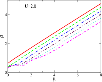
Figure 1: (Color online) Variation of average density $\rho$ as a function of the chemical potential $\mu$ for U=2, but for different values of $\lambda$ starting from 0.5 (red solid curve) to 5.5 (magenta double dash dot curve) at the intervals of 1.0.

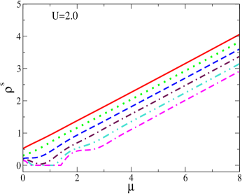
Figure 2: (Color online) Variation of average superfluid density $\rho^{s}$ as a function of $\mu$ for the same set of parameters as in Fig. 1.

III Results

Taking the superlattice potential for the two distinguished sites within the unit cell $\lambda_{1}=0$ and $\lambda_{2}=\lambda$, we present our results for a wide range of $\lambda$, densities $\rho$ and four characteristic values of the on-site interaction $U$, chosen to cover a substantial part of the phase diagram. In our analysis we have taken $t=1.0$, so all other quantities are expressed in units of $t$.

First we investigate the effect of the superlattice potential on the superfluid phase. In the Figs. 1 and 2, we plot, respectively, for $U=2$ the average density $\rho$ and the superfluid density $\rho^{s}$ as a function of the chemical potential $\mu$ for different values of $\lambda$ starting from $0.5$ to $5.5$ at an interval of $1.0$. Here $\rho$ and $\rho^{s}$ are, respectively, the average density and the superfluid density of a unit cell, i.e., $\rho=(\rho_{1}+\rho_{2})/2$, $\rho^{s}=(\phi^{2}_{1}+\phi^{2}_{2})/2$. It is known that for $U=2$, $\lambda=0$, the model (1) is always in the superfluid phase sheshadri irrespective of the value of the density $\rho$.

From the Figs. 1 and 2, we find that density $\rho$ increases with increase in $\mu$ for finite, but small values of $\lambda$. The superfluid density $\rho^{s}$ remains finite for all densities which imply that the system continues to be in the superfluid phase as in the case of $\lambda=0$. However, as $\lambda$ is increased further, say for example, $\lambda=4.5$, the density develops a plateau at $\rho=1/2$ for a range of $\mu$ values. This is the signature of a finite gap in the energy spectrum in this range of $\mu$ values and vanishing of compressibility $\kappa=\frac{\partial\rho}{\partial\mu}$. The Fig. 2 suggest vanishing of superfluid density in the same range of $\mu$. For all other densities, i.e., $\rho\neq 1/2$, including integer densities, the superfluid density remains finite. These features confirm that, for $U=2$, model (1) is in the superfluid phase for all values of $\rho\neq 1/2$ for all values of $\lambda$. However, for $\rho=1/2$ there is a superfluid to an insulator phase transition as $\lambda$ is increased.

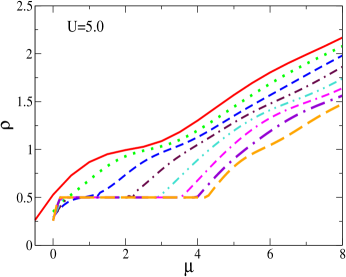
Figure 3: (Color online) Variation of average density of a unit cell $\rho$ as a function of the chemical potential $\mu$ for U=5, but for different values of $\lambda$ starting from 0.2 (red solid curve) to 7.2 (orange large dashed curve) at intervals of 1.0.

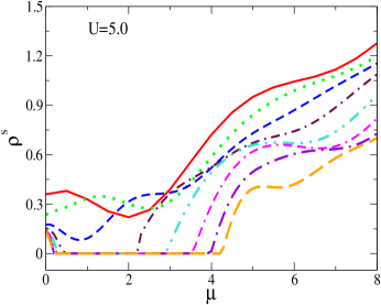
Figure 4: (Color online) Variation of average superfluid density of a unit cell as a function of $\mu$ for the same set of parameters as in Fig. 3.

Table 1: $U=2.0$

$\lambda$	$\rho$	$\mu$	$\rho^{s}_{1}$	$\rho^{s}_{2}$	$n_{1}$	$n_{2}$
0.5	0.620	0.00	0.58	0.45	0.73	0.51
0.5	1.022	0.70	0.87	0.75	1.12	0.92
0.5	2.017	2.60	1.72	1.57	2.13	1.91
1.5	0.490	0.20	0.52	0.21	0.77	0.21
1.5	1.020	1.20	0.98	0.62	1.32	0.71
1.5	2.020	3.10	1.87	1.41	2.34	1.69
2.5	0.490	0.47	0.39	0.08	0.91	0.08
2.5	1.030	1.71	1.11	0.49	1.53	0.53
2.5	2.030	3.61	2.02	1.26	2.57	1.49
3.5	0.500	0.70	0.07	0.01	0.99	0.01
3.5	1.020	2.10	1.14	0.33	1.70	0.34
3.5	2.030	4.10	2.16	1.10	2.79	1.28
4.5	0.500	0.40	0.00	0.00	1.00	0.00
4.5	1.000	2.40	1.08	0.19	1.82	0.19
4.5	2.000	4.50	2.24	0.91	2.96	1.03
5.5	0.500	0.30	0.00	0.00	1.00	0.00
5.5	1.000	2.60	0.89	0.10	1.91	0.10
5.5	2.000	5.00	2.36	0.77	3.18	0.84

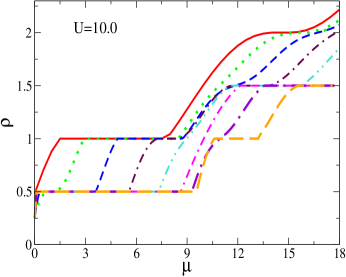
Figure 5: (Color online) Variation of average density of a unit cell $\rho$ as a function of the chemical potential $\mu$ for U=10, but for different values of $\lambda$, varying from 0.2 (red solid curve) to 14.2 (orange large dashed curve) at intervals of 2.0

This insulator phase is different from the standard Mott insulator phase arising due to the on-site interaction. Here $U=2$ is small and the Mott insulator phase is not expected. The reason for the formation of an insulator phase for $U=2$ is due to the superlattice potential, and to distinguish this insulator from the Mott insulator phase, we call it as superlattice induced Mott insulator (SLMI) arya as mentioned earlier. In order to understand the SLMI phase, the distribution of bosons within the unit cell is tabulated in the Table 1. As we discussed in the previous section, the unit cell consists of $2^{d}$ sites and each cell has two distinct sites, which we refer to as 1 and 2. The values of site densities $\rho_{1}$, $\rho_{2}$ and superfluid densities $\rho^{s}_{1}$, $\rho^{s}_{2}$ are listed in the table for different values of $\lambda$. For $\lambda<3.7$, the on-site superfluid densities $\rho^{s}_{1}$ and $\rho^{s}_{2}$ remain finite for all densities. However, for $\lambda\geq 3.7$ and density $\rho=1/2$, we find $\rho^{s}_{1}=\rho^{s}_{2}=0$ and $\rho_{1}=1,~{}\rho_{2}=0$. This implies, within the unit cell, one site is occupied and the other site being empty. Since this unit cell repeats to cover the entire lattice, it has every alternate site occupied and the other is empty like a charge density wave (CDW) phase which normally arises due to the nearest neighbor interaction. However, it should be noted here in this work that the CDW like density distribution is due to the superlattice potential and there is no nearest neighbor interaction involved. Since the distribution of bosons follow a pattern $[1~{}~{}0~{}~{}1~{}~{}0~{}~{}1~{}~{}0~{}~{}\cdots]$ in all the $d$ directions of the lattice, we call this phase as SLMI-I to distinguish it from SLMI-II discussed below. The Table 1 also confirms that there is no insulating phase for densities $\rho=1$ and $2$.

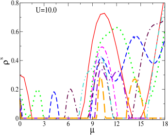
Figure 6: (Color online) Variation of average superfluid density of a unit cell as a function of $\mu$ for the same set of parameters as in Fig. 5.

Table 2: $U=5.0$

$\lambda$	$\rho$	$\mu$	$\rho^{s}_{1}$	$\rho^{s}_{2}$	$n_{1}$	$n_{2}$
0.2	0.523	0.0	0.370	0.35	0.57	0.48
0.2	1.030	2.5	0.270	0.26	1.03	1.02
0.2	2.080	7.5	1.190	1.17	2.09	2.06
2.2	0.500	0.9	0.110	0.06	0.95	0.06
2.2	1.010	3.3	0.433	0.36	1.13	0.90
2.2	2.000	8.1	1.250	1.09	2.19	1.81
3.2	0.500	0.5	0.000	0.00	1.00	0.00
3.2	1.000	3.8	0.570	0.42	1.22	0.78
3.2	2.010	8.7	1.350	1.08	2.30	1.73
4.2	0.500	0.2	0.000	0.00	1.00	0.00
4.2	0.990	5.3	0.790	0.29	1.65	0.34
4.2	2.010	10.2	1.540	0.91	2.62	1.40
7.2	0.500	0.2	0.000	0.00	1.00	0.00
7.2	1.010	5.8	0.620	0.18	1.82	0.20
7.2	2.020	10.7	1.54	0.83	2.73	1.30

Results for $U=5$ are similar to those of $U=2$. In Figs. 3 and 4 we plot, respectively, density $\rho$ and the superfluid density $\rho^{s}$ as a function of $\mu$ for different values of $\lambda$. The system is in the superfluid phase at $\rho=1/2$ and $\rho=1$ initially for low values of $\lambda$ ($<2.6$). For $\lambda>2.6$, a plateau appears in the $\rho$ versus $\mu$ plot for $\rho=1/2$ suggesting a gap in the energy spectrum. The superfluid density vanishes in this region. This plateau at $\rho=1/2$ widens as $\lambda$ increases. However, the system remains in the SF phase at $\rho=1$ for all the values of $\lambda$ considered. In Table 2, we tabulate the values of site densities and superfluid densities within the cell and we conclude that the transition from the SF to the SLMI-I phase is at $\lambda=2.6$, when the superfluid density vanishes, and the occupancy configuration is of the form [1 0 1 0 $\cdots$ ]. On the other hand, at other values of $\rho$ and for all values of $\lambda$, the superfluid densities, $\rho^{s}_{1}$ and $\rho^{s}_{2}$, remain finite.

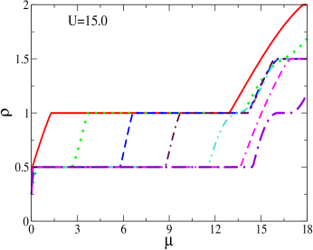
Figure 7: (Color online) Variation of average density of a unit cell $\rho$ as a function of the chemical potential $\mu$ for U=15, but for different values of $\lambda$, varying from 0.2 (red solid curve) to 18.2 (violet large dot dashed curve) at intervals of 3.0

Table 3: $U=10.0$

$\lambda$	$\rho$	$\mu$	$\rho^{s}_{1}$	$\rho^{s}_{2}$	$n_{1}$	$n_{2}$
0.2	0.48	0.00	0.30	0.29	0.53	0.44
0.2	1.00	2.00	0.00	0.00	1.00	1.00
0.2	2.00	14.50	0.00	0.00	2.00	2.00
2.2	0.50	1.20	0.00	0.00	1.00	0.00
2.2	1.00	3.00	0.00	0.00	1.00	1.00
2.2	2.00	15.00	0.00	0.00	2.00	2.00
6.2	0.50	0.50	0.00	0.00	1.00	0.00
6.2	1.00	7.50	0.00	0.00	1.00	1.00
6.2	1.50	12.00	0.00	0.00	2.00	1.00
10.2	0.50	0.19	0.00	0.00	1.00	0.00
10.2	1.00	9.97	0.65	0.32	1.51	0.47
10.2	1.50	12.16	0.00	0.00	2.00	1.00
14.2	0.50	0.10	0.00	0.00	1.00	0.00
14.2	1.00	10.70	0.00	0.00	2.00	0.00
14.2	1.50	15.60	0.00	0.00	2.00	1.00

Results for $U=10$ are different from that of $U=5$. This difference is mainly due to the fact that model (1) has SF to MI transitions for integer densities. For $\rho=1$, the critical $U_{c}\sim 5.8$ for the SF-MI transition sheshadri and this implies that for $U=10$, model (1) is in the Mott insulator phase for $\rho=1$. In the Figs. 5 and 6 we plot, respectively, density $\rho$ and the superfluid density $\rho^{s}$ as a function of $\mu$ for different values of $\lambda$. From these figures the following conclusions are drawn. For small values of $\lambda$, the plateau in the $\rho$ versus $\mu$ plot exist only for $\rho=1$ and the $\rho^{s}$ vanishes in the same range of $\mu$ confirming the expected SF to MI transition for $\rho=1$. The system remains in the superfluid phase for all other densities. However, as we increase $\lambda$, the plateau region at $\rho=1$ , i.e., the MI region, shrinks first, completely disappears for some values of $\lambda$, and re-appears again for higher values of $\lambda$.

A plateau develops at $\rho=1/2$ for $\lambda>2.3$ and at $\rho=3/2$ for $\lambda>5.3$. From the tabulated values of $\rho_{1}$ and $\rho_{2}$ in the Table 3, the insulator phase at $\rho=1/2$ is the same as SLMI-I. The insulator phase at $\rho=3/2$ has a density distribution [2 1 2 1 $\cdots$ ] which we call SLMI-III. The insulator phase at $\rho=1$ for higher values of $\lambda$ has the occupation at alternate lattice sites [2 0 2 0 $\cdots$] which we refer to as the SLMI-II phase.

Thus for $U=10.0$, for $\lambda<2.3$ the system exhibits a Mott insulator phase for $\rho=1$ and SF phase else where. For $2.3<\lambda<5.3$, the system has two insulating phases: SLMI-I for $\rho=1/2$ and MI phase for $\rho=1$. The system is in the superfluid phase for the rest of the densities. For $\lambda>5.3$ the system shows SLMI-I for $\rho=1/2$, MI phase for $\rho=1$, SLMI-III for $\rho=3/2$ and SF for other densities. For $\rho=1$ the MI phase is lost for $\lambda>6.5$ and re-appears as SLMI-II for $\lambda>13.1$. The results for $U=10.0$ are in qualitative agreement with those obtained using DMRG arya .

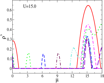
Figure 8: (Color online) Variation of average superfluid density of a unit cell as a function of $\mu$ for the same set of parameters as in Fig. 7.

Table 4: U=15.0

$\lambda$	$\rho$	$\mu$	$\rho^{s}_{1}$	$\rho^{s}_{2}$	$n_{1}$	$n_{2}$
0.2	0.52	0.10	0.28	0.28	0.57	0.47
0.2	1.00	1.30	0.00	0.00	1.00	1.00
0.2	2.00	17.80	0.00	0.00	2.00	2.00
6.2	0.50	0.18	0.00	0.00	1.00	0.00
6.2	1.00	6.66	0.00	0.00	1.00	1.00
6.2	1.50	16.11	0.00	0.00	2.00	1.00
15.2	0.50	0.10	0.00	0.00	1.00	0.00
15.2	1.02	15.10	0.60	0.30	1.55	0.49
18.2	0.50	0.09	0.00	0.00	1.00	0.00
18.2	1.0	16.00	0.00	0.00	2.00	0.00
18.2	1.50	19.08	0.00	0.00	2.00	1.00

The system for $U=15.0$ behaves similarly as $U=10.0$. At $\rho=1/2$, the system starts off in the gapless SF phase for low values of $\lambda(=0.2)$, as evident from the Figs. 7 and 8 and Table 4. But at $\rho=1.0$ and $2.0$, the system is in the MI phase at this value of $\lambda$. As $\lambda$ is increased to a value greater than $2.2$, a gap appears at $\rho=1/2$, marking the transition from the SF to the SLMI-I phase, as seen in the Table 4, where we have vanishing superfluid densities, and also a occupancy configuration of $[1~{}0~{}1~{}0~{}\cdots]$. Also, at $\rho=3/2$, another gap appears at $\lambda=4.8$, implying the transition from the SF phase to the gapped SLMI-III phase with a configuration $[2~{}1~{}2~{}1~{}\cdots]$. As $\lambda$ becomes greater than $11.7$, the system at $\rho=1.0$ undergoes a phase transition from the MI to the SF phase, shown by the non-zero values of the superfluid density. As $\lambda$ becomes larger than $18.1$, the gap reappears once again, showing that the system has entered into the gapped SLMI-II phase with configuration $[2~{}0~{}2~{}0~{}\cdots]$.

IV Conclusions

We have analyzed the various phases exhibited by a system of bosons in an optical superlattice with a unit cell consisting of two distinct lattice sites using the mean-field decoupling approximation, for various values of the superlattice potential, $\lambda$, corresponding to four values of the on-site interaction $U$. For $U=2.0$, we find that the system resides in the SF phase for all densities for small values of $\lambda$. At $\rho=1/2$, there is a transition from the SF to the SLMI-I phase at $\lambda=3.7$, but for other densities, it remains in the gapless SF phase. For $U=5.0$, the system undergoes a SF - SLMI-I phase transition for $\rho=1/2$ at $\lambda=2.6$, but remains in the SF phase for other densities and $\lambda$. For $U=10.0$, the system undergoes a SF - SLMI-I phase transition at $\lambda=2.3$ for $\rho=1/2$,. However, for $\rho=1$, the system starts in the MI phase, as the value of $U$ is large, and as $\lambda$ is increased, the gap in the MI phase shrinks, and eventually goes to zero, marking the MI-SF phase transition at $\lambda=6.5$. The system stays in the gapless SF phase for $6.5<\lambda<13.1$. As $\lambda$ is increased further the system undergoes a phase transition from SF - SLMI-II at $\lambda=13.1$. For $\rho=3/2$, we see a phase transition from SF to SLMI-III phase at $\lambda=5.3$. Similar behavior is observed for $U=15.0$, with the system for $\rho=1/2$ undergoing a phase transition at $\lambda=2.2$. For $\rho=1$, the system makes a transition from the MI to the SLMI-I phase at $\lambda=11.7$, and then from the SF to the SLMI-II phase at $\lambda=18.1$. Also a phase transition from the SF to the SLMI-III phase at $\lambda=4.8$. It should be possible to extend this calculation to superlattices with different periodicity. The charge density wave order in the SLMI phase will depend on the number of distinct sites within the unit cell. The mean field approach is exact in the infinite dimension and the error, because of neglecting the fluctuations, become severe in low dimensions rvpaispin1 . However, it proves to be an excellent tool for the qualitative analysis (e.g. phase diagram), which is our focus in this paper. Since the parameters of the Hamiltonian can be varied to a large range of values by tuning the strength of the optical potentials, we hope our detailed study of model (1) will stimulate experimental studies that could lead to the observation of the superlattice induced Mott insulators.

V Acknowledgement

R.V.P. acknowledges financial support from CSIR and DST, India. We also acknowledge useful discussions with Tapan Mishra and Gora Shlyapnikov.

References

- (1) K. Sheshadri, H. R. Krishnamurthy, R. Pandit, and T. V. Ramakrishnan, Europhys. Lett. 22, 257 (1993).
- (2) D. Jaksch, C. Bruder, J. I. Cirac, C. W. Gardiner and P. Zoller, Phys. Rev. Lett. 81, 3108 (1998).
- (3) M.P.A. Fisher, P.B. Weichmann, G. Grinstein and D.S. Fisher, Phys. Rev. B 40, 546 (1989).
- (4) M Greiner, O. Mandel, T. Esslinger, T. W. Hansch and I. Bloch, Nature 415, 39 (2002).
- (5) M. Lewenstein, A. Sanpera, V. Ahufinger, B. Damski, A. Sen De and U. Sen, Advances in Physics, Vol. 56, 243 (2007).
- (6) I. Bloch, J. Dalibard and W. Zwerger, Rev. Mod. Phys. 80, 885 (2008).
- (7) V. I. Yukalov, Laser Physics, Vol. 19, 1 (2009).
- (8) D. van Oosten, P. van der Straten, and H. T. C. Stoof, Phys. Rev. A 63, 053601 (2001).
- (9) R. V. Pai, K.Seshadri and R. Pandit , Current topics in atomic, molecular an optical physics, edited by C. Sinha and S. Bhattacharyya, World Scientific, p.105, 2007.
- (10) W. Krauth, M. Caffarel, and J. P. Bouchaud, Phys. Rev. B 45, 3137 (1992).
- (11) D. S. Rokhsar and B. G. Kotliar, Phys. Rev. B 44 10328 (1991).
- (12) Bo-Lun Chen, Su-Peng Kou, Yunbo Zhang, and Shu Chen, Phys. Rev. A 81, 053608 (2010).
- (13) V. G. Rousseau, D. P. Arovas, M. Rigol, F. Hebert, G. G. Batrouni and R. T. Scalettar, Phys. Rev. B 73, 174516 (2006).
- (14) R. Roth, K. Burnett, Phys. Rev. A 68, 023604 (2003).
- (15) Felix Schmitt, Markus Hild, and Robert Roth, arXiv:1005.3129v1 [cond-mat.quant-gas].
- (16) G. Roux, T. Barthel, I. P. McCulloch, C. Kollath, U. Schollwöck, and T. Giamarchi, Phys. Rev. A 78, 023628 (2008).
- (17) A. Dhar, T. Mishra, R. V. Pai, B. P. Das, Phys. Rev. A 83 053621 (2011).
- (18) S. Piel, J. V. Porto, B. Laburthe Tolra, J. M. Obrecht, B. E. King, M. Subbotin, S. L. Rolston and W. D. Phillips, Phys. Rev. A 67, 051603(R) (2003).
- (19) J. Sebby-Strabley, M. Anderlini, P. S. Jessen and J. V. Porto, Phys. Rev. A 73, 033605 (2006).
- (20) P. Cheinet, S. Trotzky, M. Feld, U. Schnorrberger, M. Moreno-Cardoner, S. Foelling and I. Bloch, Phys. Rev. Lett. 101, 090404 (2008).
- (21) R. V. Pai, K. Sheshadri and R. Pandit, Phys. Rev. B 77, 014503 (2008).