Abstract

The force-assisted desorption kinetics of a macromolecule from adhesive surface is studied theoretically, using the notion of tensile (Pincus) blobs, as well as by means of Monte-Carlo (MC) and Molecular Dynamics (MD) simulations. We show that the change of detached monomers with time is governed by a differential equation which is equivalent to the nonlinear porous medium equation (PME), employed widely in transport modeling of hydrogeological systems. Depending on the pulling force and the strength of adsorption, three kinetic regimes can be distinguished: (i) “trumpet” (weak adsorption and small pulling force), (ii) “stem-trumpet” (weak adsorption and moderate force), and (iii) “stem” (strong adsorption and large force). Interestingly, in all regimes the number of desorbed beads $M(t)$, and the height of the first monomer (which experiences a pulling force) $R(t)$ above the surface follow an universal square-root-of-time law. Consequently, the total time of detachment $\langle\tau_{d}\rangle$, scales with polymer length $N$ as $\langle\tau_{d}\rangle\propto N^{2}$. Our main theoretical conclusions are tested and found in agreement with data from extensive MC- and MD-simulations.

1 Introduction

During the last decade the progress in single-molecule manipulation techniques such as atomic force spectroscopy (AFM) and optical or magnetic tweezers [1] has attracted the interest of researchers to a new field of fascinating phenomena like DNA unzipping [2, 3, 4], or forced-induced detachment of individual polymers from adsorbing surfaces [5]. One can experimentally test elastic and adhesive properties as well as bond scission in polymer fibers, or in fundamental biological objects like proteins, nucleic acids, or molecular motors with spatial resolution in the nm range and force resolution in the pN range. In this way substantial progress has been achieved in the understanding and use of fibers, adhesives or biopolymers. Besides technological relevance, the field of single-chain manipulation poses also numerous questions of interest to fundamental physics. Thus, it has been shown, for example, that the force-induced unzipping of the double-stranded DNA is a $1$-st order phase transition [2, 3, 6, 7] that has the same nature as the force-induced desorption transition of a polymer from an adhesive substrate [8, 9, 10, 11] and that both phenomena can be described by the same kind of re-entrant phase diagram.

While the theoretical understanding of these phase transformations in terms of equilibrium statistical thermodynamics has meanwhile significantly improved [11], their kinetics has been so far less well explored. Originally, a theoretical treatment of the problem was suggested by Sebastian [6] while the first computer simulations of the related phenomenon of DNA force-induced unzipping were reported by Marenduzzo et al. [7]. Yet a number of basic questions pertaining to the dependence of the total mean detachment time $\langle\tau_{d}\rangle$ on polymer length $N$, pulling force $f$, or adhesion strength, $\epsilon_{s}$, remain open or need validation. So far we are not aware of computer simulational studies which would shed light on these problems. Therefore, in order to fill the gap regarding force-induced desorption kinetics, we consider in this work a generic problem: the force-induced detachment dynamics of a single chain, placed on adhesive structureless plane.

The theoretical method which we used is different and more general then in Ref. [6] where a phantom (Gaussian) chain was treated in terms of the corresponding Rouse equation. Instead, our consideration: (i) takes into account all excluded-volume interactions among monomers and, (ii) is based on the tensile-blob picture, proposed many years ago by Brochard-Wyart [12] as theoretical framework for the description of a steady-state driven macromolecule in solutions. This approach was generalized recently by Sakaue [13, 14] for the analysis of non-equilibrium transient regimes in polymer translocations through a narrow pore.

Very recently, Sebastian et al. [15] demonstrated (within the tensile blob picture) that the average position $x(n,t)$ of a monomer $n$ at time $t$ is governed by the so-called $p$-Laplacian nonlinear diffusion equation [16]. In contrast, in the present paper we discuss force-induced desorption kinetics on the basis of a nonlinear diffusion equation which governs the time-dependent density distribution $\rho(x,t)$ of monomers. We show that this equation is similar to the porous medium equation (PME) [17] which has gained widespread acceptance in the theory of groundwater transport through geological strata [18]. The most natural way of solving the PME is based on self-similarity which implies that the governing equation is invariant under the proper space and time transformation [17, 18]. Thus, self-similarity reduces the problem to a nonlinear ordinary differential equation which can be solved much more easily.

Eventually, in order to check our predictions we performed extensive MD- and MC-simulations which, for the case of strong adsorption, large pulling forces and overdamped regime, show an excellent agreement with our theoretical predictions. Moreover, the comparison of MC and MD data reveals that the presence of inertial effects, typical in underdamped dynamics, significantly affects the observed detachment kinetics.

The paper is organized as follows: after this short introduction, in Section 2 we present briefly the theoretical treatment of the problem and emphasize the different regimes pertinent to polymer detachment kinetics. A short description of the simulational MC- and MD models is given in Section 3 while in Section 4 we discuss the main results provided by our computer experiments. In Section 5 we suggest a plausible experiment which could validate our theoretical results. We end this work by a brief summary of our findings in Section 6.

2 Tensile-blob picture for the force-induced detachment

2.1 Trumpet regime

2.1.1 Beads density temporal variation is described by a nonlinear porous medium equation

After equilibration on an attractive solid substrate, the adsorbed polymer chain can be pictured as a two dimensional string of adsorption blobs of size $D\propto a(\epsilon_{s}-\epsilon_{c})^{-\nu/\phi}$ [19], where $a$ is the Kuhn segment length, and $\nu$ and $\phi$ are respectively the Flory exponent and the crossover (or, adsorption) exponent. The dimensionless adsorption energy $\epsilon_{s}=\varepsilon_{s}/k_{B}T$ (here and in what follows $k_{B}$ denotes the Boltzmann constant, and $T$ is temperature), whereas $\epsilon_{c}$ is the critical adsorption point (CAP). The external driving force $f$ acts on the free chain end (in the $x$-direction) while the second chain end is tethered to the substrate. If the pulling force strength falls in the range $1/N^{\nu}\ll af/k_{B}T\leqslant 1$, the chain tail forms a kind of “trumpet” shape, as shown schematically in Fig. 1a. Moreover, as far as the adsorption blob, adjacent to “trumpet”, changes its lateral position (i.e., its coordinates within the substrate) during desorption, the “trumpet” has not only vertical velocity (in the $x$-direction) but also a lateral one. The latter leads to a tilt of the “trumpet” axis in direction opposite to the lateral velocity due to Stokes friction. The tilting angle is denoted by $\theta$ in Fig.  1 and, as will be seen from our simulation results in Sec. 4, almost does not change in the course of detachment. This substantially simplifies the theoretical consideration.

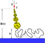
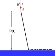
Figure 1: The picture of the single adsorbed chain detachment. The chain is initially equilibrated, giving rise to a string of adsorption blobs with a blob size $D$. The external driving force $f$, exerted on the first monomer, is switched on at the initial time moment. By time $t$ the position of the first monomer is denoted as $R(t)$. The shaded part of the chain displays a tensile blobs sequence which has a form of a “trumpet”, tilted opposite to the lateral velocity direction by angle $\theta$. a) The “trumpet” regime, corresponding to weak adsorption and weak pulling force, i.e., $1/N^{\nu}\ll{\widetilde{\varphi}}<{\widetilde{f}}<1$. b) The “stem” regime, corresponding to strong adsorption and strong pulling force, $1\ll{\widetilde{\varphi}}<{\widetilde{f}}$. c) The “Stem-trumpet” regime, representing the intermediate pulling force interval ${\widetilde{\varphi}}<1<{\widetilde{f}}$.

Let us denote by $f(x,t)$ the tensile force which acts in direction of the “trumpet” axis at an arbitrary cross-section of a tensile (Pincus) blob, placed at distance $x$ from the substrate at time $t$. The $x$-component of this tensile force reads $f_{x}(x,t)=f(x,t)\cos\theta$. The blob size is then given by

$$\xi(x,t)=\dfrac{k_{B}T}{f(x,t)}=\dfrac{Ck_{B}T}{f_{x}(x,t)}$$ (1)

where $C=\cos\theta$. It can be seen from Fig. 1a that the size of the tensile blob at $x$ corresponds to the lateral size of the polymer at height $x$. The balance of forces in $x$-direction at this point yields

$$f_{x}(x,t)=\gamma\>\int\limits_{D}^{x}\>v_{x}(x^{\prime},t)\>\left[\dfrac{\xi(x^{\prime},t)}{a}\right]^{z-2}\dfrac{dx^{\prime}}{\xi(x^{\prime},t)}+\varphi$$ (2)

where $v_{x}(x,t)$ is the $x$-component of the local velocity and $\varphi$ is the restoring force which is exerted on the moving domain by the last adsorption blob. The value of $\varphi$ depends on the proximity to the critical point $\epsilon_{c}$ as well as on the chain model itself (see below). In the integral in Eq. (2), $dx^{\prime}/\xi(x^{\prime},t)$ counts the number of blobs in the interval $x^{\prime},x^{\prime}+dx^{\prime}$ whereas $\gamma\>v_{x}(x^{\prime},t)\>[\xi(x^{\prime},t)/a]^{z-2}$ is the local Stokes friction force ($\gamma$ being the friction coefficient) [20]. The dynamic exponent equals either $z=2+1/\nu$, or $z=3$, for Rouse- and Zimm dynamics respectively. Thus, taking into account Eq. (1), the equation for the blob size reads

$$\xi(x,t)=\dfrac{Ck_{B}T}{\gamma\>\int_{D}^{x}\>v_{x}(x^{\prime},t)\>\left[\xi(x^{\prime})/a\right]^{z-2}dx^{\prime}/\xi(x^{\prime})+\varphi}.$$ (3)

With this equation one may represent the local velocity $v(x,t)$ in terms of the blob size $\xi(x,t)$ as

$$v_{x}(x,t)=-\dfrac{Ck_{B}T}{a\gamma}\>\left[\dfrac{a}{\xi(x,t)}\right]^{z-1}\>\dfrac{\partial\xi(x,t)}{\partial x}.$$ (4)

The local (linear) monomer density $\rho(x,t)$ and the local blob size $\xi(x,t)$ are related by $\rho(x,t)=[\xi(x,t)/a]^{(1-\nu)/\nu}/a$ so that Eq. (4) can be written in the form

$$v_{x}(x,t)=-\dfrac{Ck_{B}T\nu}{\gamma(1-\nu)}\>\dfrac{1}{[{\widetilde{\rho}}(x,t)]^{\nu(z-2)/(1-\nu)+1}}\>\dfrac{\partial{\widetilde{\rho}}(x,t)}{\partial x},$$ (5)

where we have introduced the notation for the dimensionless monomer density ${\widetilde{\rho}}(x,t)=a\rho(x,t)$.

The local flux of polymer beads has a standard form $J_{x}(x,t)=v_{x}(x,t)\>\rho(x,t)$, that is,

$$J_{x}(x,t)=-\dfrac{\nu Ck_{B}T}{a\gamma(1-\nu)[{\widetilde{\rho}}(x,t)]^{\nu(z-2)/(1-\nu)}}\>\dfrac{\partial}{\partial x}\>{\widetilde{\rho}}(x,t)$$ (6)

With $J_{x}(x,t)$ from Eq. (6), one may determine ${\widetilde{\rho}}(x,t)$ from the continuity equation $\partial\rho(x,t)/\partial t=-\partial J_{x}(x,t)/\partial x$:

$$\dfrac{\partial{\widetilde{\rho}}}{\partial{\widetilde{t}}}\>=\dfrac{\partial}{\partial{\widetilde{x}}}\left({\widetilde{\rho}}^{m-1}\dfrac{\partial{\widetilde{\rho}}}{\partial{\widetilde{x}}}\right)$$ (7)

where we have introduced the dimensionless (tilded) independent variables ${\widetilde{x}}=x/a$ and ${\widetilde{t}}=t/\tau_{0}$ (thereby the characteristic time is $\tau_{0}=a^{2}\gamma(1-\nu)/\nu Ck_{B}T$). Eq. (7) has the form of the nonlinear porous medium equation (PME) [17] where the characteristic exponent $m=-[\nu(z-1)-1]/(1-\nu)$ has in our case a negative value. An equation similar to PME has been discussed recently by Sakaue et al. [21] in the context of polymer expansion and unfolding from a compact state. In this case the consideration has been based on the dynamics of concentration blobs [20] rather than tensile blobs like here. This kind of nonlinear partial differential (parabolic) equations is commonly used in the context of groundwater infiltration or seepage through porous strata [18] where the exponent $m>1$.

The geometric factor $C=\cos\theta$ is unessential in the subsequent consideration and we will drop it. In addition to Eq. (7), one has to fix the initial and boundary conditions (BC). Initially, there are no polymer segments at $x>D$, so that

$${\widetilde{\rho}}(x,t=0)=0$$ (8)

At $x=D$ the tensile blob is equal in size to the adsorption blob, i.e., $\xi(x=D,t)=k_{B}T/\varphi$. As a result, in terms of the dimensionless density, one has

$${\widetilde{\rho}}({\widetilde{x}}={\widetilde{D}},t)=\dfrac{1}{{\widetilde{\varphi}}^{(1-\nu)/\nu}}$$ (9)

where ${\widetilde{D}}=D/a$ and ${\widetilde{\varphi}}=a\varphi/k_{B}T$.

The BC on the moving end of the “trumpet” follows from the condition $\xi(x=R(t),t)=k_{B}T/f$ which corresponds to the smallest blob size, i.e.,

$${\widetilde{\rho}}({\widetilde{x}}={\widetilde{R}}(t),t)=\dfrac{1}{{\widetilde{f}}^{(1-\nu)/\nu}}$$ (10)

Here again the dimensionless quantities, ${\widetilde{R}}(t)=R(t)/a$ and ${\widetilde{f}}=af/k_{B}T$, are introduced.

Our consideration is based on the assumption that the lateral component of the tensile force is very weak (because the trumpet is almost vertical), so that any force propagation along the adsorbed part of chain can be neglected. This is different from the case considered by Serr and Netz [22] where the pulling of a strongly adsorbed chain by means of an AFM has been investigated. In contrast to the present case where an uniform field pulls on the first bead, the AFM cantilever can move vertically and horizontally with respect to substrate so that the tilt angle $\theta$ changes with time. Moreover, in this case the sliding of the polymer on the substrate becomes important with the polymer-surface friction force being much larger than the Stokes friction force for the detached part which is essential in our case. Therefore, the AFM can not be actually used for testing the scheme shown in Fig. 1. In Sec. 5 we will discuss a plausible electrostatic tracking experiment which makes it possible, in principle, to test a gentle detachment even close to the adsorption critical point.

2.1.2 Self-similar solution

In the same manner as for the PME, the solution of Eq. (7) is derived by symmetry of self-similarity (SS). This symmetry implies invariance of the solution with respect to the stretching transformation : ${\widetilde{t}}\rightarrow\eta{\widetilde{t}}$ , ${\widetilde{x}}\rightarrow\eta^{\delta}{\widetilde{x}}$, ${\widetilde{\rho}}\rightarrow\eta^{\omega}{\widetilde{\rho}}$. The requirement that Eq. (7) stays invariant under the stretching transformation connects the exponents $\omega,m$, and $\delta$ by the following relation [17]

$$\omega(1-m)+2\delta=1$$ (11)

On the other hand, this requirement also fixes the self-similar form of the solution as

$${\widetilde{\rho}}({\widetilde{x}},{\widetilde{t}})=t^{\omega}\>W(u),\quad u=({\widetilde{x}}-{\widetilde{D}})/{\widetilde{t}}^{\delta}.$$ (12)

In Eq. (12), $W(u)$ is a scaling function and we took into account that at ${\widetilde{t}}=0$ ${\widetilde{x}}={\widetilde{D}}$. On the other hand, the boundary condition given by Eq. (9) is compatible with the SS-form Eq. (12) only if $\omega=0$. Then, as a consequence of Eq. (11), $\delta=1/2$. Substituting Eq. (12) into (7) yields a nonlinear ordinary differential equation for the scaling function $W(u)$, i.e.,

$$\dfrac{d}{du}\left(W^{m-1}\dfrac{d}{du}W\right)+\dfrac{u}{2}\dfrac{d}{du}W=0$$ (13)

The BC given by Eq. (9) reads

$$W(u=0)=\dfrac{1}{{\widetilde{\varphi}}^{(1-\nu)/\nu}}$$ (14)

Assume now that the moving chain end follows the scaling relation ${\widetilde{R}}({\widetilde{t}})={\widetilde{D}}+{{\widetilde{v}}_{d}}{\widetilde{t}}^{\chi}$ where $\chi$ is an exponent and the factor ${\widetilde{v}}_{d}$ will be fixed below. This scaling ansatz is compatible with the BC given by Eq. (10) only if $\chi=1/2$. This imposes the boundary condition

$$W(u={\widetilde{v}}_{d})=\dfrac{1}{{\widetilde{f}}^{(1-\nu)/\nu}}$$ (15)

Finally, the initial condition Eq. (8) becomes

$$W(u=\infty)=0$$ (16)

The nonlinear Eq. (13) may be solved numerically. However, in case the pulling force $f$ exceeds the restoring force only by a small amount, one can show (see below) that ${\widetilde{v}}_{d}\ll 1$, i.e., the interval of argument $u$ variation, where $W(u)$ is nonzero, is very narrow. As a result, $0\leq u\leq{\widetilde{v}}_{d}\ll 1$ and one can linearize Eq. (13) (by making use Eq. (14)) to get

$${\widetilde{\varphi}}^{z-2}\dfrac{d^{2}}{du^{2}}W(u)+\dfrac{u}{2}\dfrac{d}{du}W(u)=0$$ (17)

where for small arguments $W(u)^{m-1}\approx{\widetilde{\varphi}}^{(z-2)}$. The solution of Eq. (17), subject to both conditions Eq. (14) and Eq. (16), is given by

$$W(u)=\dfrac{1}{{\widetilde{\varphi}}^{(1-\nu)/\nu}}\left[1-{\rm erf}\left(\dfrac{u}{2{\widetilde{\varphi}}^{(z-2)/2}}\right)\right]$$ (18)

where ${\rm erf}(x)=(2/\sqrt{\pi})\int_{0}^{x}\exp(-t^{2})dt$ is the error function.

The chain end velocity amplitude, ${\widetilde{v}}_{d}$, can be determined now from the condition Eq. (15). If the pulling force ${\widetilde{f}}$ is only slightly larger than the restoring force ${\widetilde{\varphi}}$, one can expand $W(u)\approx[1-u/(\pi^{1/2}{\widetilde{\varphi}}^{(z-2)/2})]/{\widetilde{\varphi}}^{(1-\nu)/\nu}$. Thus, one obtains

$${\widetilde{v}}_{d}\simeq\sqrt{\pi}\>{\widetilde{\varphi}}^{(z-2)/2}\left[1-\left(\dfrac{{\widetilde{\varphi}}}{{\widetilde{f}}}\right)^{(1-\nu)/\nu}\right]$$ (19)

The equation of motion for the moving end then reads

$${\widetilde{R}}({\widetilde{t}})={\widetilde{D}}+\sqrt{\pi}{\widetilde{\varphi}}^{(z-2)/2}\left[1-\left(\dfrac{{\widetilde{\varphi}}}{{\widetilde{f}}}\right)^{(1-\nu)/\nu}\right]\sqrt{\widetilde{t}}$$ (20)

The variation of the number of desorbed monomers with time, $M(t)$, is given by the integral

$$M(t) = \int\limits_{D}^{R(t)}\>\rho(x,t)\;dx=\sqrt{{\widetilde{t}}}\>\int\limits_{0}^{{\widetilde{v}}_{d}}\;W(u)du$$ (21)

$$\simeq \sqrt{\pi}{\widetilde{\varphi}}^{(z\nu-2)/2\nu}\left[1-\left(\dfrac{{\widetilde{\varphi}}}{{\widetilde{f}}}\right)^{(1-\nu)/\nu}\right]\sqrt{{\widetilde{t}}}$$

Eventually, the total time for polymer detachment, $\langle\tau_{d}\rangle$, reads

$$\langle\tau_{d}\rangle=\dfrac{\tau_{0}N^{2}}{\pi{\widetilde{\varphi}}^{(z\nu-2)/2\nu}\left[1-({\widetilde{\varphi}}/{\widetilde{f}})^{(1-\nu)/\nu}\right]^{2}}$$ (22)

Combining Eqs. (21) and (22), one obtains the following dynamical scaling law

$$M(t)=N\sqrt{\dfrac{{\widetilde{t}}}{\langle\tau_{d}\rangle}}$$ (23)

Eventually, we would like to stress that in the foregoing consideration one neglects the thermal fluctuations so that the necessary condition for desorption requires that ${\widetilde{f}}>{\widetilde{\varphi}}$. On the other hand, the “trumpet” formation is only possible when $1/N^{\nu}\ll{\widetilde{f}}<1$. Therefore, the “trumpet” regime holds, provided that

$$1/N^{\nu}\ll{\widetilde{\varphi}}<{\widetilde{f}}<1,$$ (24)

which means that then one deals with weak adsorption and weak pulling force.

2.2 Dependence of the restoring force $\varphi$ on the adsorption energy $\epsilon_{s}$

One can write the restoring force in scaling form, $\varphi=\frac{k_{B}T}{a}{\cal F}(\epsilon_{s})$, with $\epsilon_{s}=\varepsilon_{s}/k_{B}T$ and ${\cal F}(x)$ - a scaling function. Force $\varphi$ stays constant in the course of the desorption process as long as at least one adsorption blob is still located on the attractive surface. The strength of $\varphi$ can be determined from the plateau in the deformation curve: force vs. chain end position [23].

In an earlier work [24], we demonstrated that the fugacity per adsorbed monomer $z^{*}(\epsilon_{s})$, which determines its chemical potential $\mu_{\rm ads}=\ln z^{*}$, can be found from the basic equation

$$\Phi(\alpha,\mu_{3}z^{*})\;\Phi(\lambda,\mu_{2}wz^{*})=1.$$ (25)

In Eq. (25) $\alpha=\phi-1$ ($\phi$ is the so-called crossover exponent which, according to the different simulation methods, ranges between $\phi\simeq 0.48$ and $\phi\simeq 0.59$; see the corresponding discussion in ref. [24] ) $\lambda=1-\gamma_{d=2}\simeq-0.343$ (where $\gamma_{d=2}$ is a universal exponent which governs the two-dimensional polymer statistics), $w=\exp(\epsilon_{s})$, $\mu_{2}$, and $\mu_{3}$ are so-called connective constants in two- and three-dimensional spaces respectively, and the polylog function $\Phi$ is defined by the series $\Phi(\alpha,y)=\sum_{n=1}^{\infty}\>y^{n}/n^{\alpha}$. The values of $\mu_{2}$, $\mu_{3}$ and $\gamma_{d=2}$ could be found in the text-book [25].

In local equilibrium $\mu_{\rm ads}$ should be equal to the chemical potential of detached monomer $\mu_{\rm det}=\dfrac{1}{k_{B}T}\;\dfrac{\partial F_{\rm str}}{\partial N}$, where $F_{\rm str}$ is the free energy of the driven polymer chain so that $\mu_{\rm ads}=\mu_{\rm det}$. The expression for $F_{\rm str}$ depends on the polymer model. The moving blob domain, shown in Fig. 1, exerts on the last adsorbed monomer a force which is equal in magnitude and opposite in sign to the restoring force $\varphi$. Therefore, the free energy of a stretched polymer within the bead-spring (BS) model is given by [24]

$$F_{\rm str}=-N\left(\dfrac{a\varphi}{k_{B}T}\right)^{1/\nu}-N\ln\mu_{3}$$ (26)

On the other hand, within the freely jointed bond vector (FJBV) model, the partition function, corresponding to $F_{\rm str}$, reads [26]

$$Z_{N}=\left(4\pi\right)^{N}\>\left(\dfrac{k_{B}T}{a\varphi}\right)^{N}\>\left[\sinh\left(\dfrac{a\varphi}{k_{B}T}\right)\right]^{N}$$ (27)

In Eq. (27) the free chain partition function $Z_{N}=\left(4\pi\right)^{N}$ for $\varphi\rightarrow 0$. A correspondence with the BS-model may be established by the substitution $4\pi\rightarrow\mu_{3}$ in Eq. (27) so that the FJBV-free energy becomes

$$F_{\rm str}=-k_{B}TN\ln\left[\mu_{3}\left(\dfrac{k_{B}T}{a\varphi}\right)\sinh\left(\dfrac{a\varphi}{k_{B}T}\right)\right]$$ (28)

Taking into account Eqs. (26) and (28), one obtains eventually

$$\dfrac{a\varphi}{T}=\begin{cases}\left[-\ln(\mu_{3}z^{*}(\epsilon_{s}))\right]^{\nu},&\mbox{BS model}\\ {\cal R}^{-1}(-\ln(\mu_{3}z^{*}(\epsilon_{s}))),&\mbox{FJBV model}\end{cases}$$ (29)

where ${\cal R}^{-1}(x)$ is the inversed of the function ${\cal R}(x)=\ln\left[\mu_{3}\sinh(x)/x\right]$ and $\mu_{3}z^{*}(\epsilon_{s})\leq 1$.

Below we consider separately the restoring force, Eq. (29), in the limits of strong and weak adsorption.

2.2.1 Strong adsorption

In the case of the strong adsorption ($\epsilon_{s}\gg 1$), the solution of Eq. (25) reads $z^{*}(\epsilon_{s})\simeq\mu_{2}^{-1}{\rm e}^{-\epsilon_{s}}$ [24], and for the BS-model one gets $a\varphi/k_{B}T\simeq\left[\epsilon_{s}+\ln(\mu_{2}/\mu_{3})\right]^{\nu}$.

For the FJBV model at $\epsilon_{s}\gg 1$ one has ${\cal R}(x)\simeq\ln\left(\mu_{3}{\rm e}^{x}/x\right)\simeq x+\ln\mu_{3}$. From Eq. (29) it then follows $a\varphi/k_{B}T+\ln\mu_{3}=\epsilon_{s}+\ln\mu_{2}$, or $a\varphi/k_{B}T\simeq\epsilon_{s}+\ln(\mu_{2}/\mu_{3}$. The final result for the restoring force in the strong adsorption limit takes on the form

$${\widetilde{\varphi}}=\begin{cases}\left[\epsilon_{s}+\ln(\mu_{2}/\mu_{3})\right]^{\nu},&\mbox{BS model}\\ \epsilon_{s}+\ln(\mu_{2}/\mu_{3}),&\mbox{FJBV model}\end{cases}$$ (30)

It is well known that under strong forces (and correspondingly strong adsorption) the FJBV-model is better suited for description of the simulation experiment results (see, e.g., Sec. 5 in our paper [23]). That is why in Eq. 30 the second line is appears as the more appropriate result.

2.2.2 Weak adsorption

Close to the critical adsorption point, the solution of Eq. (25) takes on the form

$z^{*}(\epsilon_{s})\simeq\mu_{3}^{-1}\left[1-C_{1}(\epsilon_{s}-\epsilon_{c})^{1/\phi}\right]$ [24], where $C_{1}$ is a constant. Then, Eq. (29) gives $a\varphi/k_{B}T\simeq C_{1}(\epsilon_{s}-\epsilon_{c})^{\nu/\phi}$ for the BS-model.

In the case of weak adsorption $a\varphi/k_{B}T$ is small and ${\cal R}(x)\simeq\ln\left[\mu_{3}(1+x^{2}/6)\right]\simeq\ln\mu_{3}+x^{2}/6$. Eq. (29) then yields $a\varphi/k_{B}T\simeq B_{1}(\epsilon_{s}-\epsilon_{c})^{1/2\phi}$, where $B_{1}$ is a constant. The unified result in the weak adsorption limit is

$${\widetilde{\varphi}}=\begin{cases}C_{1}\left(\epsilon_{s}-\epsilon_{c}\right)^{\nu/\phi},&\mbox{BS model}\\ B_{1}(\epsilon_{s}-\epsilon_{c})^{1/2\phi},&\mbox{FJBV model}\end{cases}$$ (31)

In fact, Eq. (31) may also be derived differently. Namely, as already mentioned, the size of an adsorption blob is given by $D=aC_{1}(\epsilon_{s}-\epsilon_{c})^{-\nu/\phi}$ whereas the size of a tensile blob $\xi(x=D)=k_{B}T/\varphi$. The condition for detachment may be set as $\xi(x=D)=D$ which leads again to Eq. (31) (whereby the dimensionless notation ${\widetilde{\varphi}}=a\varphi/k_{B}T$ has been used). On the other hand, the relationship between $D$ and $\varphi$, written as $D\varphi/k_{B}T\simeq 1$, leads to the adsorption blob size for the FJBV-model: $D\sim(\epsilon_{s}-\epsilon_{c})^{-1/2\phi}$ (where the second line in Eq. (31) has been used).

2.3 Stem and stem-trumpet regimes

For strong, $1<a\varphi/k_{B}T<af/k_{B}T$, and moderate, $a\varphi/k_{B}T<1<af/k_{B}T$, detachment force $f$ one has to consider the “stem”(see Fig. 1b) and “stem-trumpet” (see Fig. 1c) regimes, respectively.

2.3.1 Stem regime

In this case the moving domain is build up from a “stem” of the length $M(t)$ (total number of desorbed monomers). The “stem” velocity is $dM(t)/dt$ (with an accuracy of the geometrical factor $C=cos\theta$ which is not important for scaling predictions), so that the balance of driving and drag forces yields

$$\gamma M(t)\>\dfrac{dM(t)}{dt}=f-\varphi$$ (32)

The solution of Eq. (32) in the dimensionless units reads

$$M(t)=\sqrt{2({\widetilde{f}}-{\widetilde{\varphi}})\>{\widetilde{t}}}$$ (33)

Evidently, this takes on the same form as Eq. (23), $M(t)=N\sqrt{{\widetilde{t}}/\langle{\widetilde{\tau}_{d}}\rangle}$, whereby the mean detachment (dimensionless) time $\langle{\widetilde{\tau}_{d}}\rangle=N^{2}/[2({\widetilde{f}}-{\widetilde{\varphi}})]$.

2.3.2 Stem-trumpet regime

The “stem-trumpet” shape of the driven polymer is shown in Fig. 1c. In this case the local density in the “trumpet” part ${\widetilde{\rho}}({\widetilde{x}},{\widetilde{t}})$ is governed by the same Eq. (7) but with a boundary condition in the junction point (i.e., in the point where the “stem” goes over into the “trumpet” part). There, the blob size is $\xi(x=R(t)-S(t),t)=a$. Thus, one gets

$${\widetilde{\rho}}({\widetilde{x}}={\widetilde{R}}(t)-{\widetilde{S}}(t),{\widetilde{t}})=1$$ (34)

The boundary condition at ${\widetilde{x}}={\widetilde{D}}$ has the same form, Eq. (9), as before. The solution again has the scaling form ${\widetilde{\rho}}({\widetilde{x}},{\widetilde{t}})=W(u)$. The moving end now follows the law ${\widetilde{R}}(t)={\widetilde{D}}+{\widetilde{S}}(t)+{\widetilde{u}}_{d}\sqrt{{\widetilde{t}}}$, where the prefactor ${\widetilde{u}}_{d}$ can be fixed by using the condition $W(u={\widetilde{u}}_{d})=1$. Consequently,

$${\widetilde{u}}_{d}=\sqrt{\pi}{\widetilde{\varphi}}^{(z-2)/2}\left[1-{\widetilde{\varphi}}^{(1-\nu)/\nu}\right]$$ (35)

In order to calculate the length of the “stem” portion, ${\widetilde{S}}(t)$, one can use the results of the previous subsection. The only difference lies in the fact that now the “stem - trumpet” junction point moves itself with velocity ${\widetilde{u}}_{d}/(2\sqrt{{\widetilde{t}}})$ and the driving force is ${\widetilde{f}}-1$. Therefore, the balance of driving and drag forces leads to the following equation for ${\widetilde{S}}(t)$

$$\left(\dfrac{{\widetilde{u}}_{d}}{2\sqrt{{\widetilde{t}}}}+\dfrac{d}{d{\widetilde{t}}}\>{\widetilde{S}}(t)\right)\>{\widetilde{S}}(t)={\widetilde{f}}-1$$ (36)

The solution of Eq. (36) reads

$${\widetilde{S}}(t)=\left[\sqrt{\dfrac{{\widetilde{u}}_{d}^{2}}{4}+2({\widetilde{f}}-1)}-\dfrac{{\widetilde{u}}_{d}}{2}\right]\>\sqrt{{\widetilde{t}}}$$ (37)

The resulting equation for the average height of the end monomer becomes

$${\widetilde{R}}(t)={\widetilde{D}}+\left[\sqrt{\dfrac{{\widetilde{u}}_{d}^{2}}{4}+2({\widetilde{f}}-1)}+\dfrac{{\widetilde{u}}_{d}}{2}\right]\>\sqrt{{\widetilde{t}}}$$ (38)

The number of desorbed monomer can be easily calculated as an integral over the the number of monomers in the “trumpet” part and in the “stem” portion, i.e.,

$$M({\widetilde{t}}) = \sqrt{{\widetilde{t}}}\>\int\limits_{0}^{{\widetilde{u}}_{d}}\>W(u)du+{\widetilde{S}}({\widetilde{t}})$$ (39)

$$= \left[\sqrt{\dfrac{{\widetilde{u}}_{d}^{2}}{4}+2({\widetilde{f}}-1)}-\dfrac{{\widetilde{u}}_{d}}{2}\left(1-\dfrac{2}{{\widetilde{\varphi}}^{(1-\nu)/\nu}}\right)\right]\>\sqrt{{\widetilde{t}}}$$

where ${\widetilde{u}}_{d}$ is given by Eq. (35). Evidently, all characteristic scales as well as the number of desorbed monomers vary in time as $\sqrt{t}$. This shows that the average desorption time $\langle\tau\rangle$ is proportional to $N^{2}$ as before.

2.4 Dynamic Regimes

The foregoing theoretical analysis was based essentially on the notion of tensile (Pincus) blobs as well as on the “quasi-static” approximation, i.e., on the equating of driving and drag forces locally (in space and time). Depending on the pulling ${\widetilde{f}}$ and restoring ${\widetilde{\varphi}}$ force strengths, one distinguishes a “trumpet” ($1/N^{\nu}\ll{\widetilde{\varphi}}<{\widetilde{f}}<1$), “stem-trumpet” (${\widetilde{\varphi}}<1<{\widetilde{f}}$ ), and a ”stem“ ($1<{\widetilde{\varphi}}<{\widetilde{f}}$) regimes (see Fig. 2). Notably, in all regimes the average number of desorbed monomers $M(t)$ and the height of the first monomer $R(t)$ evolve as a $\sqrt{t}$-time universal law. Moreover, the evolution equation which governs the polymer beads density $\rho(x,t)$ in the tensile blobs is analogous to the nonlinear porous medium equation which is commonly used for investigations of gas and fluid infiltration in the geological porous strata [17, 18]. Following this line we have demonstrated that the scaling analysis of such equation, based on symmetry of self-similarity, immediately brings about a $\sqrt{t}$-time universal law.

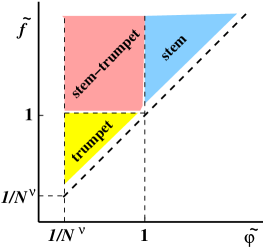
Figure 2: Different dynamic regimes of forced polymer chain desorption in terms of pulling ${\widetilde{f}}$ and restoring ${\widetilde{\varphi}}$ forces. The relation between ${\widetilde{\varphi}}$ and the adsorption energy $\epsilon_{s}$ is given by Eq. (30) and Eq. (31) for the strong and weak adsorption, respectively. The white strip along the diagonal indicates that in all cases the condition ${\widetilde{f}}>{\widetilde{\varphi}}$ is important.

The value of ${\widetilde{\varphi}}$ depends on the adsorption energy $\epsilon_{s}$ and is described by different expressions, depending on the particular polymer chain model: bead-spring (BC), or freely jointed bond vectors (FJBV) models. For large adsorption energy ($\epsilon_{s}\gg 1$), the restoring force is also large, leading to the ”stem“ regime. Close to the the critical adsorption point (for vanishing adhesion), the restoring force could attain a very small value, leading to a ‘trumpet”, or “stem-trumpet” regimes. In this case the role of fluctuations, which was neglected in our theoretical investigation, becomes important and could result in correction to the basic $\sqrt{t}$-time law.

In the next section we will give results of our MC- and MD-simulation study that were carried out in some of the foregoing forced-desorption (mainly ”stem“) regimes.

3 Computational Models

3.1 Monte-Carlo

We have used a coarse grained off-lattice bead spring model to describe the polymer chains. Our system consists of a single chain tethered at one end to a flat structureless surface while the external pulling force is applied to other chain end. In the MC simulation the surface attraction of the monomers is described by a square well potential $U_{w}(x)=-\epsilon_{s}$ for $x<\delta=0.125$ and $U_{w}(x)=0$ otherwise. Here the strength $\epsilon_{s}/k_{B}T$ is varied from $0.6$ to $3.6$. The effective bonded interaction is described by the FENE (finitely extensible nonlinear elastic) potential.

$$U_{\mbox{\tiny FENE}}=-K(1-l_{0})^{2}\ln\left[1-\left(\frac{l-l_{0}}{l_{max}-l_{0}}\right)^{2}\right]$$ (40)

with $K=20,l_{max}=1,l_{0}=0.7,l_{min}=0.4$

The non-bonded interactions between the monomers are described by the Morse potential.

$$\frac{U_{M}(r)}{\epsilon_{M}}=\exp(-2\alpha(r-r_{min}))-2\exp(-\alpha(r-r_{min}))$$ (41)

with $\alpha=24,\;r_{min}=0.8,\;\epsilon_{M}/k_{B}T=1$. This model is currently well established and has been used due to its reliability and efficiency in a number of studies [27] of polymer behavior on surfaces.

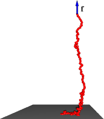
Figure 3: Snapshots from a MC simulation of chain with $N=128$, adsorbed on a solid plane with energy of adsorption $\epsilon_{s}/k_{B}T=3.0$. (a) at time $t=0$ before, and (b) - after a pulling force $f=3.0$ is applied perpendicular to substrate.

We employ periodic boundary conditions in the $y-z$ directions and impenetrable walls in the $z$ direction. The lengths of the studied polymer chains are typically $64$, $128$, and $256$. The size of the simulation box was chosen appropriately to the chain length, so for example, for a chain length of $128$, the box size was $256\times 256\times 256$ . All simulations were carried out for constant force. A force $f$ was applied to the last monomer in the $x$-direction, i.e., perpendicular to the adsorbing surface

The standard Metropolis algorithm was employed to govern the moves with self avoidance automatically incorporated in the potentials. In each Monte Carlo update, a monomer was chosen at random and a random displacement was attempted with $\Delta x,\;\Delta y,\;\Delta z$ chosen uniformly from the interval $-0.5\leq\Delta x,\Delta y,\Delta z\leq 0.5$. The transition probability for the attempted move was calculated from the change $\Delta U$ of the potential energies before and after the move as $W=\exp(-\Delta U/k_{B}T)$. As for standard Metropolis algorithm, the attempted move was accepted, if $W$ exceeds a random number uniformly distributed in the interval $[0,1]$. As a rule, the polymer chains have been originally equilibrated in the MC method for a period of about $10^{6}$ MCS (depending on degree of adsorption $\epsilon_{s}$ and chain length $N$ this period is varied) whereupon one performs $200$ measurement runs, each of length $8\times 10^{6}$ MCS. Various properties of the chain are then sampled during the course of the run. The starting configuration is replaced by a new sequence in the beginning of the next run. Two typical snapshots of chain configurations, immediately before the detachment starts, and some time later, are presented in Fig. 3.

3.2 Molecular Dynamics

In our MD-simulations we use a coarse-grained model of a polymer chain of $N$ beads connected by finitely extendable elastic bonds. The bonded interactions in the chain is described by the frequently used Kremer-Grest potential, $V^{\mbox{\tiny KG}}(r)=V^{\mbox{\tiny FENE}}(r)+V^{\mbox{\tiny WCA}}(r)$, with FENE potential, Eq. (40), and a non-bonded repulsion term taken as Weeks-Chandler-Anderson (WCA) (i.e., the shifted and truncated repulsive branch of the Lennard-Jones potential) given by

$$V^{\mbox{\tiny WCA}}(r)=4\epsilon\left[(\sigma/r)^{12}-(\sigma/r)^{6}+1/4\right]\theta(2^{1/6}\sigma-r)$$ (42)

with $\theta(x)=0$ or 1 for $x<0$ or $x\geq 0$, and $\epsilon=1$, $\sigma=1$. The potential $V^{\mbox{\tiny KG}}(r)$ has got a minimum at bond length $r_{\mbox{\tiny bond}}\approx 0.96$.

The substrate in the present investigation is considered simply as a structureless adsorbing plane, with a Lennard-Jones potential acting with strength $\epsilon_{s}$ in the perpendicular $x$–direction, $V^{\mbox{\tiny LJ}}(x)=4\epsilon_{s}[(\sigma/x)^{12}-(\sigma/x)^{6}]$.

The dynamics of the chain is obtain by solving a Langevin equation of motion for the position $\mathbf{r}_{n}=[x_{n},y_{n},z_{n}]$ of each bead in the chain,

$$m\ddot{\mathbf{r}}_{n}=\mathbf{F}_{n}^{j}+\mathbf{F}_{n}^{\mbox{\tiny WCA}}-\gamma\dot{\mathbf{r}}_{n}+\mathbf{R}_{n}(t)+\mathbf{f}_{n}\delta_{nN},\qquad(n,\ldots,N)$$ (43)

which describes the Brownian motion of a set of bonded particles whereby the last of them is subjected to external (constant) stretching force $\mathbf{f}=[f,0,0]$. The influence of solvent is split into slowly evolving viscous force and rapidly fluctuating stochastic force. The random, Gaussian force $\mathbf{R}_{n}$ is related to friction coefficient $\gamma$ by the fluctuation-dissipation theorem. The integration step is $0.002$ time units (t.u.) and time in measured in units of $\sqrt{m\sigma^{2}/\epsilon}$, where $m$ denotes the mass of the beads, $m=1$. The ratio of the inertial forces over the friction forces in Eq. (43) is characterized by the Reynolds number ${\rm Re}=\sqrt{m\epsilon}/\gamma\sigma$ which in our simulation falls in the range ${\rm Re}=0.1\div 4$. In the course of simulation velocity-Verlet algorithm is used to integrate equations of motion (43).

4 Simulation results

In order to check the validity of our theoretical predictions, we carried out extensive computer simulations by means of both Monte-Carlo (MC) and Molecular Dynamics (MD) so that a comparison can be made between the overdamped dynamics of a polymer (MC) and the behavior of an inertial (underdamped) system (MD). For ultimate consistency of the data, we performed also MD simulations with very large friction coefficient $\gamma=10$ whereby the obtained data was found to match that from the MC computer experiment.

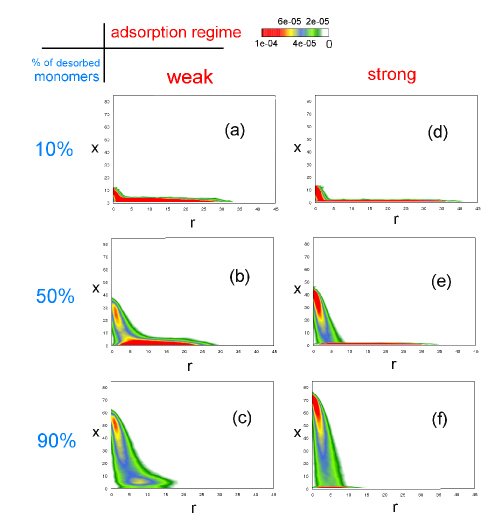
Figure 4: Polymer density distributions of beads plotted for different adsorption regimes: (a)–(c) $\epsilon_{s}/(k_{B}T)=1.9$, (d)–(f) $\epsilon_{s}/(k_{B}T)=5.0$ and various percentage of detached monomers ($10\%$, $50\%$ and $90\%$). The $x$-axis coincides with direction of pulling force whereas $r=\sqrt{(y_{1}-y_{n})^{2}+(z_{1}-z_{n})^{2}}$, $(n=1,\ldots,N)$ is the radial component of beads calculated with respect to the first monomer. Here $N=100$, $T=0.1$ and $\gamma=0.25$.

First of all, it would be interesting to verify that trumpet-like structures, which have been discussed thoroughly in Sec.2, can be seen in our MD-simulation experiment. Figure 4 represents such a visualization where the beads density distributions are given (as a function of $x$-coordinate as well as the radial coordinate calculated with respect to the first monomer, i.e. $r=\sqrt{(y_{1}-y)^{2}+(z_{1}-z)^{2}}$) for the weak , $\epsilon_{s}/k_{B}T=1.9$, (left panel) and strong, $\epsilon_{s}/k_{B}T=5$, (right panel) adsorptions. Each density plot was implemented as a result of averages over many runs under the fixed fraction of desorbed monomers: $10\%$ (upper row), $50\%$ (middle row) and $90\%$ (bottom row). As one can see, the moving domain is developed into the trumpet-like configuration in both, weak and strong adsorption, cases. Moreover, the ”trumpet“ is tilted as it was argued in Sec. 2.1.1 due to its lateral velocity and the corresponding Stokes friction. An important point is that the tilt angle stays constant which substantially simplifies the theoretical consideration in Sec. 2.1.1. Recall that the density in the blob $n_{b}(x)$ and the blob size $\xi(x)$ are related as $n_{b}(x)\propto 1/[\xi(x)]^{3-1/\nu}\propto 1/[\xi(x)]^{1.3}$, i.e., the larger the density is, the smaller blob size. This tendency can be seen in Fig. 4 where the most dense portion (red color) comes close to the tip of the ”trumpet“ as it should be. Moreover, for the strong adsorption case (see Fig. 4d-f) this most dense portion becomes more extended which might mean a ”stem-trumpet“ formation. As a result, the density plots, given in Fig. 4, provide a good evidence for the existence of the trumpet-like structures, suggested and discussed in Sec. 2.

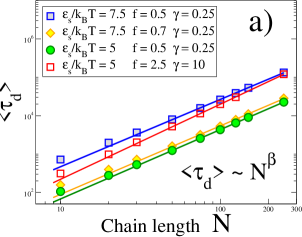
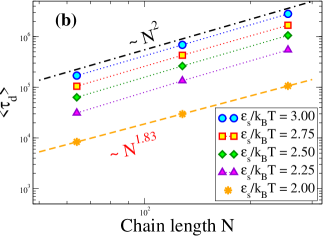
Figure 5: (a) MD data for the mean desorption time $\langle\tau_{d}\rangle$ of a chain vs chain length $N$, plotted for different strength of pulling force $f$, adhesion strength $\epsilon_{s}/k_{B}T$, and friction $\gamma$. Symbols denote the results of simulation while solid lines represent fitting curves $\langle\tau_{d}\rangle\propto N^{\beta}$ which were found in the range $N=50\div 250$. The value of the exponent $\beta$ depends on the dynamics: underdamped $\beta\approx 1.75\pm 0.1$ (full symbols) and overdamped $1.96\pm 0.03$ (empty symbols). (b) Variation of $\langle\tau_{d}\rangle$ with $N$ at different strength of adhesion $\epsilon_{s}/k_{B}T$ from the MC data. Note that here the critical adsorption energy $\epsilon_{c}/k_{B}T\approx 2.0$. In the strong adsorption regime $\beta=2.0$, whereas close to the critical point $\beta=1.83$.

As one of our principal results, it was found that the chain length dependence of the mean detachment time $\langle\tau_{d}\rangle$ follows a scaling law $\langle\tau_{d}\rangle\sim N^{\beta}$, Fig. 5, where $\beta$, the detachment exponent, depends on the type of dynamics (underdamped or overdamped) as well as on the adsorption strength (i.e., on the proximity of $\epsilon_{s}$ to the adsorption critical point, $\epsilon_{c}$). Fig. 5a shows result from the MD-simulation for different values of $\epsilon_{s}$, the pulling force $f$, and the friction coefficient $\gamma$. For the underdamped dynamics, one finds a detachment exponent $\beta=1.75\pm 0.1$ whereas for the overdamped one $\beta=1.96\pm 0.03$. The last value is very close to the theoretical prediction which immediately follows from Eq. (33), $\langle\tau_{d}\rangle\propto\tau_{0}N^{2}/({\widetilde{f}}-{\widetilde{\varphi}})$, i.e., $\beta=2$. Recall that this theoretical prediction neglects any effects of inertia and describes overdamped dynamics. In addition, detachments are considered in the ”stem“ scenario, that is, for relatively large adsorption energy and pulling force.

This conclusion is supported by the MC-simulation results (which represent the overdamped limit) shown in Fig. 5b. For the relatively strong adsorption one finds $\beta=2.02\pm 0.01$, which is very close to the theoretical prediction. On the other hand, in the vicinity of the adsorption critical point the detachment exponent appears to be smaller $\beta=1.83\pm 0.01$. Indeed, one may suggest that the observed decrease is due to fluctuations which become stronger close to $\epsilon_{c}$. As mentioned above, fluctuations are not taken into account in our theoretical treatment which is based on the ”quasistatic“ approximation. As a matter of fact, in the cases of ”trumpet“ and ”stem-trumpet“ scenarios (relatively weak adsorption energy and pulling force), the fluctuations alter the value of the detachment exponent so that $\beta<2$. It is, however, conceivable too that $\beta=1.83$ may also be due to finite-size effects in the vicinity of the critical adsorption point where the size of adsorption blobs becomes large.

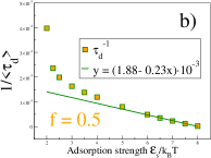
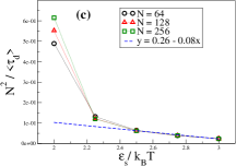
Figure 6: MD data on the inverse mean desorption time $1/\langle\tau_{d}\rangle$ of a chain with $N=50$ plotted as a function of: a) pulling force $f$, and b) adsorption strength $\epsilon_{s}/k_{B}T$. Here $\gamma=0.25$. c) Inverse mean detachment time $N^{2}/\langle\tau_{d}\rangle$ (scaled with $N^{2}$) against $\epsilon_{s}$ from MC data with $f=3.0$ and $\epsilon_{s}/k_{B}T=3.0$.

In order to check the $f-$ and $\epsilon_{s}-$dependence of $\langle\tau_{d}\rangle$, which the relation $\langle\tau_{d}\rangle\propto\tau_{0}N^{2}/({\widetilde{f}}-{\widetilde{\varphi}})$ predicts for the the ”stem“ regime, we have plotted $1/\langle\tau_{d}\rangle$ vs. $f$, Fig. 6a, and vs. $\epsilon_{s}$, Fig. 6b. In Fig.  6a one can see a perfect straight line as expected. As for the $\epsilon_{s}$-dependence, we recall that according to Eq. (30), in the strong adsorption limit the restoring force ${\widetilde{\varphi}}\approx c_{1}(\epsilon_{s}+c_{2})$ where $c_{1}$ and $c_{2}$ are some constants. As can be seen from Fig. 6b, in the MD-simulation this holds for $\epsilon_{s}>5$. On the other hand, in the MC simulation, the strong adsorption regime starts at $\epsilon_{s}>2.5$ as is evident from Fig. 6c.

Fig. 7 demonstrates the validity of the $\sqrt{t}$-law for the time evolution of the mean number of desorbed monomers, $M(t)$, given by Eq. (33). According to this relationship, the quantity $\gamma M^{2}(t)/(f-\varphi)$ should be a linear function of time.

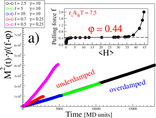
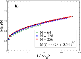
Figure 7: (a) Mean squared number of desorbed monomers $\gamma M^{2}(t)/[(f-\varphi)]$ for a chain composed of $N=100$ particles shown as a function of time for different sets of $f$ and $\gamma$ - MD data. Here $\epsilon_{s}/k_{B}T=5.0$. The inset displays the (equilibrium) relationship between pulling force $f$ and the resulting mean height $\langle H\rangle$ of the first monomer in a chain with $N=50$. The estimated value of the plateau height (which is the restoring force in the course of detachment) is $\varphi=0.44$. (b) Variation of $M(t)$ with (dimensionless) elapsed time (measured in units of $t/\langle\tau_{d}\rangle$) for different polymer lengths $N$ from MC data. Here $\epsilon_{s}/k_{B}T=3.0$. Dashed line denotes the expected $\sqrt{t}$-behavior, cf. Eq. (33).

In order to fix the value of the restoring force $\varphi$, we have carried out an independent simulation to find how the mean height of the first monomer $\langle H\rangle$ depends in equilibrium on the pulling force $f$ for a previously adsorbed (end-grafted) chain. The result of this is shown as an inset in Fig. 7a where the value of plateau height yields the restoring force $\varphi=0.44$ at adsorption energy $\epsilon_{s}=5.0$. By making use of this value we were able to superimpose three curves for different forces, $f=2.5,\;5,\;10$ in the overdamped case ($\gamma=10.0$) on a single master curve as shown in Fig. 7a. Evidently, in the case of underdamped dynamics this collapse on a single master curve does not work. This deviation from the theoretical predictions indicates again that they apply perfectly only to the case of overdamped dynamics. Finally, the respective $M(t)$ vs. time relationship from the MC-simulation is shown in Fig. 7b. One should thereby note that in the starting equilibrium configuration of the adsorbed chain about 24% of the monomers reside in loops so they are actually desorbed even before the pulling force is applied. Evidently, as in the MD data for very large friction, the curves for different chain lengths collapse on a single master $\sqrt{t}$-curve in agreement with Eq. (33).

5 Plausible experimental validation

Now we are in a position to discuss how the detachment kinetics considered in this paper could be validated in a laboratory experiment. To this end we recall that using conventional AFM, optic (OT), or magnetic tweezers (MT), the tracking is performed by practically macroscopic, of micrometers large, agents: by cantilever in AFM, or by e.g. polystyrene beads in OT and MT cases. On the other hand, the trumpet-like structures are the result of delicate interplay between pulling and drag (or friction) forces. Obviously, the Stokes friction of the cantilever as that of the polystyrene beads exceeds largely the friction of the tested polymer chain itself and thus suppresses the observation of the predicted time-behavior. One could solve this problem only if the the tracking agent is of the size of a single monomer, e.g., when it is a charged ionic end-group like a carboxylate group placed in an external electric field. Moreover, the polymer end should be fluorescently labeled in order to measure the polymer end spatial location.

One way to do this is by means of total internal reflection fluorescence microscopy (TIRFM) which is a powerful technique aimed at imaging fluorescent species close to an interface  [28]. A possible schematic setup is shown in Fig. 8

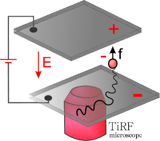
Figure 8: Schematic representation of micromanipulation (detachment) experiment using TIRF microscope.

First of all, let us estimate the required tracking forces. In the strong adsorption limit $a\varphi/k_{B}T\simeq 0.5$. The Boltzmann constant $k_{B}=1.4\cdot 10^{-23}$ J/K, the temperature $T=300$ K, a bond length $a=10^{-10}$ m so as a result $\varphi=2.1\cdot 10^{-11}$ N $=21$ pN. In the case of weak adsorption, $\varphi\simeq(k_{B}T/aN^{\nu})$, that is, for $N=10^{3}$ one has $\varphi\simeq 8.4\cdot 10^{-13}$ N $\approx 1$ pN. As a result, one deals typically with forces $1$ pN $\leq\varphi\leq 20$ pN.

Now, one could estimate which electric field $E$ should be applied to electrodes, of the capacitor shown in Fig. so as to produce a tracing force $1\;pN$. The tracking force is $f=qE$, where $q$ is the charge of the ionic end-group. The typical ion charge $q=1.6\cdot 10^{-19}$ C , so that for $E=5\cdot 10^{6}$ V/m one gets $f=5\cdot 1.6\cdot 10^{-19}\cdot 10^{6}\approx 10^{-12}$ N $=1$ pN. This value of the electrical field is much smaller than the dielectric strength of benzene, $E_{st}=165\cdot 10^{6}$ V/m, or even of distilled water $E_{st}=70\cdot 10^{6}$  V/m [29], i.e., these fluids could be used as dielectrics between the plates of the capacitor. We underline that a totally stretched polymer of chain length, say $N=10^{3}$, has a characteristic size of hundred nanometers, so that the distance between plates of the capacitor should not be larger than $1\div 10\mu m$. This means that in order to create the electric field $E=5\cdot 10^{6}$ V/m one should apply to the capacitor a voltage $5\div 50$ V, i.e., no high-voltage facility are necessary.

From a chemical point of view, the sample represents a substrate with end-grafted polymers at a low graft density (i.e., the chains are in a ”mushroom“ conformation). The synthesis of, e.g., polystyrene end-grafted chains could be performed by surface-initiated radical polymerization [30], followed by the labeling of the other chain end through carboxyl groups and fluorescent dyes. These estimations show that an electrostatic tracking experiment provides a way to test and verify our main theoretical results.

6 Conclusion

In this work we consider the force-induced desorption of a polymer from a structureless adhesive surface both analytically and by means of two distinct methods for computer simulation.

We have shown theoretically that there are three dynamical regimes of a polymer chain detachment. Depending on the pulling ${\widetilde{f}}$ and restoring ${\widetilde{\varphi}}$ forces, one can discriminate between a ”trumpet“ ($1/N^{\nu}\ll{\widetilde{\varphi}}<{\widetilde{f}}<1$), ”stem-trumpet“ (${\widetilde{\varphi}}<1<{\widetilde{f}}$), and ”stem“ ($1<{\widetilde{\varphi}}<{\widetilde{f}}$) regimes of desorption.

Remarkably, in all these cases the time dependence of the number of desorbed monomers $M(t)$ and the height of the first monomer (i.e., the monomer which experiences the applied external pulling force) $R(t)$ follows an universal $\sqrt{t}$-law (even though this is not a diffusion phenomenon). There is, however, a common physical background with the well-known Lucas-Washburn $\sqrt{t}$-law of capillary filling [31] as with the ejection kinetics of a polymer chain from a cavity (virus capsid) [32]. In these seemingly different phenomena there is always a constant driving force (meniscus curvature, or polymer entropy) which acts against a gradually changing drag force (friction) in the course of the process.

We discovered an interesting similarity between the differential equation governing the monomer density variation $\rho(x,t)$ in time and space, and the nonlinear porous medium equation (PME) [17, 18]. This makes it possible to use the self-similarity property of PME and derive rigorously the $\sqrt{t}$-law.

Our extensive MD- and MC-simulations of the detachment kinetics support this finding as well as the $\langle\tau_{d}\rangle\propto N^{\beta}$ scaling with $\beta=2$ of mean detachment time $\tau_{d}$ with chain length $N$. The theoretically predicted dependence of $\langle\tau_{d}\rangle$ on pulling force $f$ and adsorption energy $\epsilon_{s}$ appears in perfect agreement with the simulation results. As noted above, the consistency between theory and computer experiment is well manifested in the case of overdamped dynamics and strong adsorption. Moreover, by means of MD-simulation we have shown that the beads density distribution plots support the notion of trumpet-like tilted tensile blob structures. One can envisage not only tilted but, e.g., bended (horn-like) structures where the local lateral velocity depends on the $x$-coordinate. We leave this more complicated case for future investigation.

The deviations in the exponent $\beta$ due to inertial effects in the underdamped dynamical regime ($\beta\approx 1.75$ found in the MD simulation) as well as close to the adsorption critical point $\epsilon_{c}$ ($\beta=1.83$, in the MC simulation) are also challenging. It appears possible that inertial effects and fluctuations close to the CAP (both neglected in our theoretical treatment) may lead to similar consequences for the dynamics of polymer desorption, manifested by the observed decrease in the detachment exponent $\beta$. In both cases this suggests that polymer detachment is facilitated. This is clearly a motivation for further studies of the problem.

Polymer Detachment from Adsorbing Surface: Theory, Simulation and Similarity to Infiltration into Porous Medium
by Jaroslaw Paturej, Andrey Milchev, Vakhtang G. Rostiashvili, and Thomas A. Vilgis

TOC graph:

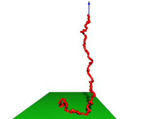
Figure 9: A snapshot from MC simulation of a partially desorbed polymer chain with $N=128$ monomers under pulling force $f=3.0$ and surface adhesion $\epsilon_{s}/k_{B}T=2.50$.

References

- [1] Ritort, F. J. Phys. Cond. Mat. 2006, 18, R531.
- [2] Bhattacharjee, S. M. J. Phys. A 2000, 33, L423.
- [3] Marenduzzo, D.; Trovato, A.; Maritan, A. Phys. Rev. E 2001, 64, 031901.
- [4] Orlandini, E.; Bhattacharjee, S.; Mernduzzo, D.; Maritan, A.; Seno, F. J. Phys. A 2001, 34, L751.
- [5] Kierfeld, J. Phys. Rev. Lett. 2006, 97, 058302.
- [6] Sebastian, K.L. Phys. Rev. E 2000, 62, 1128.
- [7] Marenduzzo, D.; Bhattacharjee, S.M; Maritan, A.; Orlandini, E.; Seno, F. Phys. Rev. Lett. 2002, 88, 028102.
- [8] Bhattacharya, S.; Rostiashvili, V. G.; Milchev, A.; Vilgis T. Phys. Rev. E 2009, 79, 030802(R).
- [9] Bhattacharya, S.; Rostiashvili, V. G.; Milchev, A.; Vilgis, T. Macromolecules 2009, 42, 2236.
- [10] Bhattacharya, S.; Milchev, A.; Rostiashvili, V. G.; Vilgis, T. Eur. Phys. J. E 2009, 29, 285.
- [11] Skvortsov A. M.; Klushin L. I.; Fleer G. J.; Leermakers, F. A. M. J. Chem. Phys. 2010, 132, 064110.
- [12] Brochard-Wyart, F. Europhys. Lett. 1993, 23, 105.
- [13] Sakaue, T. Phys. Rev. E 2007, 76, 021803.
- [14] Sakaue, T. Phys. Rev. E 2010, 81, 041808.
- [15] Sebastian, K.L.; Rostiashvili, V.G.; Vilgis, T.A.; EPL 2011, 95, 48006.
- [16] Simsen, J.; Gentile, C.B. Nonlinear Anal. 2009, 71, 4609.
- [17] Vázquez, J.L. The Porous Medium Equation, Clarendon Press, Oxford, 2007.
- [18] Barenblatt, G.I.; Entov, V.M.; Ryzhik, V.M. Theory of Fluid Flows Through Natural Rocks, Kluwer Academic Publishers, London, 1990.
- [19] de Gennes, P.G.; Pincus, P. J. Phys, (France) Lett. 1983, 44, L241.
- [20] de Gennes, P.G. Scaling Concept in Polymer Physics, Cornell University Press, Ithaca, 1979.
- [21] Sakaue, T.; Yoshinaga, N. Phys. Rev. Lett. 2009, 102, 148302
- [22] Serr, A.; Netz, R. Europhys. Lett. 2006, 73, 292.
- [23] Bhattacharya, S.; Milchev, A.; Rostiashvili, V.G.; Vilgis, T.A. Eur. Phys. J. E 2009, 29, 285.
- [24] Bhattacharya, S.; Milchev, A.; Rostiashvili, V.G.; Vilgis, T.A. Macromolecules 2009, 42, 2236.
- [25] Vanderzande, C. Lattice Model of Polymers, Cambridge University Press, Cambridge, 1998.
- [26] Sheng, Y.-J.; Lai P.-Y. Phys. Rev. E 1997, 56, 1900.
- [27] Milchev, A.; Binder, K. Macromolecules 1996 29, 343.
- [28] Mashanov G.I.; Tacon D.; Knight A.E.; Peckham M.; Molloy J. E. Methods, 2003, 29, 142.
- [29] CRC Handbook of Chemistry and Physics, 93rd Edition, 2012-2013.
- [30] Y. Tsujii, K. Ohno, S. Yamamoto, A. Goto, T. Fukuda, Adv. Polym. Sci. 2006, 197, 1.
- [31] Dimitrov, D. I.; Klushin, L.; Milchev, A.; Binder, K. Phys. Fluids2008, 20, 092102.
- [32] Milchev, A.; Klushin, L.; Skvortsov, A.; Binder K. Macromolecules 2010, 43, 6877.