A Quasi-Variational Inequality Problem
Arising in the Modeling of Growing Sandpiles

Abstract

Existence of a solution to the quasi-variational inequality problem arising in a model for sand surface evolution has been an open problem for a long time. Another long-standing open problem concerns determining the dual variable, the flux of sand pouring down the evolving sand surface, which is also of practical interest in a variety of applications of this model. Previously, these problems were solved for the special case in which the inequality is simply variational. Here, we introduce a regularized mixed formulation involving both the primal (sand surface) and dual (sand flux) variables. We derive, analyse and compare two methods for the approximation, and numerical solution, of this mixed problem. We prove subsequence convergence of both approximations, as the mesh discretization parameters tend to zero; and hence prove existence of a solution to this mixed model and the associated regularized quasi-variational inequality problem. One of these numerical approximations, in which the flux is approximated by the divergence-conforming lowest order Raviart–Thomas element, leads to an efficient algorithm to compute not only the evolving pile surface, but also the flux of pouring sand. Results of our numerical experiments confirm the validity of the regularization employed.

AMS subject classifications. 35D30, 35K86, 35R37, 49J40, 49M29, 65M12, 65M60, 82C27

Key words. Quasi-variational inequalities; critical-state problems; primal and mixed formulations; finite elements; existence; convergence analysis.

1 Introduction

Let a cohesionless granular material (sand), characterized by its angle of repose $\alpha$, be poured out onto a rigid surface $y=w_{0}(\underline{x})$, where $y$ is vertical, $\underline{x}\in\Omega\subset\mathbb{R}^{d}$, $d=1$ or 2, and $\Omega$ is a domain with boundary $\partial\Omega$. The support surface $w_{0}\in W^{1,\infty}_{0}(\Omega)$ and the nonnegative density of the distributed source $f\in L^{2}(0,T;L^{2}(\Omega))$ are given. We consider the growing sandpile $y=w(\underline{x},t)$ and set an open boundary condition $w|_{\partial\Omega}=0$. Denoting by $\underline{q}(\underline{x},t)$ the horizontal projection of the flux of material pouring down the evolving pile surface, we can write the mass balance equation

$$\frac{\partial w}{\partial t}+\underline{\nabla}\,.\,\underline{q}=f.$$ (1.1)

The quasi-stationary model of sand surface evolution, see Prigozhin [16, 17, 18], assumes the flow of sand is confined to a thin surface layer and directed towards the steepest descent of the pile surface. Wherever the support surface is covered by sand, the pile slope should not exceed the critical value; that is, $w>w_{0}\ \Rightarrow\ |\underline{\nabla}w|\leq k_{0}$, where $k_{0}=\tan\alpha$ is the internal friction coefficient. Of course, the uncovered parts of support can be steeper. This model does not allow for any flow on the subcritical parts of the pile surface; that is, $|\underline{\nabla}w|<k_{0}\ \Rightarrow\ \underline{q}=\underline{0}$. These constitutive relations can be conveniently reformulated for a.e. $(\underline{x},t)\in\Omega\times(0,T)$ as

$$|\underline{\nabla}w|\leq M(w)\qquad\mbox{and}\qquad M(w)\,|\underline{q}|+\underline{\nabla}w\,.\,\underline{q}=0,$$ (1.2)

where for any $\underline{x}\in\overline{\Omega}$

$$M(w)(\underline{x}) :=\left\{\begin{array}[]{ll}k_{0}&w(\underline{x})>w_{0}(\underline{x}),\\ \max(k_{0},|\underline{\nabla}w_{0}(\underline{x})|)&w(\underline{x})\leq w_{0}(\underline{x}).\end{array}\right.$$ (1.5)

Let us define, for any $\eta\in C(\overline{\Omega})$, the closed convex non-empty set

$$K(\eta):=\left\{\varphi\in W^{1,\infty}_{0}(\Omega)\ :\ |\underline{\nabla}\varphi|\leq M(\eta)\ \ \mbox{a.e. in}\ \Omega\right\}.$$ (1.6)

Since $M(w)\,|\underline{q}|+\underline{\nabla}\varphi\,.\,\underline{q}\geq 0$ for any $\varphi\in K(w)$, we have, on noting (1.2), that $w\in K(w)$ and $\underline{\nabla}(\varphi-w)\,.\,\underline{q}\geq 0$. A weak form of the latter inequality is: for a.a. $t\in(0,T)$

$$\int_{\Omega}\underline{\nabla}\,.\,\underline{q}\,(w-\varphi)\,{\rm d}\underline{x}\geq 0\qquad\forall\ \varphi\in K(w).$$ (1.7)

Combining (1.7) and (1.1) yields an evolutionary quasi-variational inequality for the evolving pile surface: Find $w\in K(w)$ such that for $a.a.\ t\in(0,T)$

$$\int_{\Omega}\left(\frac{\partial w}{\partial t}-f\right)(\varphi-w)\,{\rm d}\underline{x}\geq 0\qquad\forall\ \varphi\in K(w).$$ (1.8)

Assuming there is no sand on the support initially, we set

$$w(\cdot,0)=w_{0}(\cdot).$$ (1.9)

A solution $w$ to this quasi-variational inequality problem, (1.8) and (1.9), if it exists, should be a monotonically non-decreasing function in time for any $f\geq 0$, see §3 in Prigozhin [18]. However, existence and uniqueness of a solution has only been proved for support surfaces with no steep slopes; that is, $|\underline{\nabla}w_{0}|\leq k_{0}$, see Prigozhin [16, 18]. In this case $K(w)\equiv K:=\left\{\varphi\in W^{1,\infty}_{0}(\Omega)\ :\ |\underline{\nabla}\varphi|\leq k_{0}\ \ \mbox{a.e. in}\ \Omega\right\}$ and the quasi-variational inequality becomes simply a variational inequality. Independently, the variational inequality for supports without steep slopes has been derived and studied in Aronson, Evans and Wu [1] as the $p\rightarrow\infty$ limit of the evolutionary $p$-Laplacian equation.

The quasi-variational inequality (1.8) can, of course, be considered not only with the initial condition (1.9). However, if $w(\cdot,0)=\widetilde{w}_{0}(\cdot)\geq w_{0}(\cdot)$ and $\widetilde{w}_{0}$ does not belong to the admissible set $K(\widetilde{w}_{0})$, an instantaneous solution reconstruction takes place. Such discontinuous solutions, interpreted as simplified descriptions of collapsing piles with overcritical slopes, were studied in the variational inequality case in Evans, Feldman and Gariepy [10], and Dumont and Igbida [8]. Since we assumed the initial condition (1.9) and, obviously, $w_{0}\in K(w_{0})$, one could expect a solution continuously evolving in time. However, for the quasi-variational inequality with the open boundary condition $w|_{\partial\Omega}=0$, an uncontrollable influx of material from outside can occur through the parts of the boundary where $\underline{\nabla}w_{0}\,.\,\underline{\nu}\geq k_{0}$, where $\underline{\nu}$ is the outward unit normal to $\partial\Omega$. This makes the solution non-unique and, possibly, discontinuous. Such an influx is prevented in our model by assuming that

$$\underline{\nabla}w_{0}\,.\,\underline{\nu}<k_{0}\ \ \mbox{on}\ \partial\Omega,$$ (1.10)

which implies that $\underline{\nabla}w\,.\,\underline{\nu}<k_{0}$ on $\partial\Omega$ for $t>0$.

For the variational inequality version of the sand model, equivalent dual and mixed variational formulations have recently been proposed; see, e.g., Barrett and Prigozhin [4] and Dumont and Igbida [7]. Such formulations are often advantageous, because they allow one to determine not only the evolving sand surface $w$ but also the surface flux $\underline{q}$, which is of interest too in various applications; see Prigozhin [15, 17], and Barrett and Prigozhin [6]. In such formulations, and this is their additional advantage, the difficult to deal with gradient constraint is replaced by a simpler, although non-smooth, nonlinearity.

Here we will also use a mixed variational formulation of a regularized version of the growing sandpile model involving both variables. Instead of excluding the surface flux $\underline{q}$ from the model formulation, as in the transition to (1.8) above, we now note that the first condition in (1.2) holds if for a.e. $(\underline{x},t)\in\Omega\times(0,T)$

$$M(w)\,|\underline{v}|+\underline{\nabla}w\,.\,\underline{v}\geq 0$$ (1.11)

for any test flux $\underline{v}$. Hence we can reformulate the conditions (1.2) for a.a. $t\in(0,T)$ as

$$\int_{\Omega}\left[M(w)\,(|\underline{v}|-|\underline{q}|)-w\,\underline{\nabla}\,.\,(\underline{v}-\underline{q})\right]{\rm d}\underline{x}\geq 0$$ (1.12)

for any test flux $\underline{v}$, and consider a mixed formulation of the sand model as (1.1) and (1.12).

The quasi-variational inequality (1.8) is a difficult problem; in particular, due to the discontinuity of the nonlinear operator $M$, which determines the gradient constraint in (1.6). Furthermore, the natural function space for the flux $\underline{q}$ is the space of vector-valued bounded Radon measures having $L^{2}$ divergence. If $\underline{q}$ is such a measure, the discontinuity of $M(w)$ also makes it difficult to give a sense to the term $\int_{\Omega}M(w)\,|\underline{q}|\,{\rm d}\underline{x}$ in the inequality (1.12) of the mixed formulation.

In this work we consider a regularized version of the growing sandpile model with a continuous operator $M_{\varepsilon}:C(\overline{\Omega})\rightarrow C(\overline{\Omega})$, determined as follows. For a fixed small $\varepsilon>0$, we approximate the initial data $w_{0}\in W^{1,\infty}_{0}(\Omega)$ by $w_{0}^{\varepsilon}\in W^{1,\infty}_{0}(\Omega)\cap C^{1}(\overline{\Omega})$, and $M(\cdot)$ by the continuous function $M_{\varepsilon}(\cdot)$ such that for any $\underline{x}\in\overline{\Omega}$

$$M_{\varepsilon}(\eta)(\underline{x})$$

$$\;:=\left\{\begin{array}[]{ll}k_{0}&\eta(\underline{x})\geq w_{0}^{\varepsilon}(\underline{x})+\varepsilon,\\ k_{1}^{\varepsilon}(\underline{x})+(k_{0}-k_{1}^{\varepsilon}(\underline{x}))\,\left(\displaystyle\frac{\eta(\underline{x})-w_{0}^{\varepsilon}(\underline{x})}{\varepsilon}\right)&\eta(\underline{x})\in[w_{0}^{\varepsilon}(\underline{x}),w_{0}^{\varepsilon}(\underline{x})+\varepsilon],\\[11.38109pt] k_{1}^{\varepsilon}(\underline{x}):=\max(k_{0},|\underline{\nabla}w_{0}^{\varepsilon}(\underline{x})|)&\eta(\underline{x})\leq w_{0}^{\varepsilon}(\underline{x}).\end{array}\right.$$ (1.16)

We note that $M_{\varepsilon}$ is such that for all $\eta_{1},\,\eta_{2}\in C(\overline{\Omega})$

$$|M_{\varepsilon}(\eta_{1})-M_{\varepsilon}(\eta_{2})|_{0,\infty,\Omega}\leq\frac{k_{1,\infty}^{\varepsilon}-k_{0}}{\varepsilon}\,|\eta_{1}-\eta_{2}|_{0,\infty,\Omega}\,,$$ (1.17)

where

$$k_{1,\infty}^{\varepsilon}:=\max_{x\in\overline{\Omega}}k_{1}^{\varepsilon}(\underline{x})\,.$$ (1.18)

In addition, it follows for any $\underline{x}\in\overline{\Omega}$ that

$$\eta_{1}(\underline{x})\geq\eta_{2}(\underline{x})\quad\Rightarrow\quad 0<k_{0}\leq M_{\varepsilon}(\eta_{1}(\underline{x}))\leq M_{\varepsilon}(\eta_{2}(\underline{x}))\leq k^{\varepsilon}_{1}(\underline{x})\,.$$ (1.19)

We note that the analysis of the sand quasi-variational inequality problem studied in this paper is far more involved than that of the superconductivity quasi-variational inequality problem studied by the present authors in [6]. In the superconductivity context, ${M}:{\mathbb{R}}\rightarrow[{M}_{0},{M}_{1}]\subset{\mathbb{R}}$ with ${M}_{0}>0$. In [6], we exploit the fact that $|\underline{\nabla}w(\underline{x})|\leq M(w(\underline{x}))$ can be rewritten as $|\underline{\nabla}[F(w(\underline{x}))]|\leq 1$ for all $\underline{x}\in\Omega$, where $F^{\prime}(\cdot)=[{M}(\cdot)]^{-1}$ and $F(0)=0$. Clearly, such a reformulation is not applicable to $M(\cdot)$, (1.5), or $M_{\varepsilon}(\cdot)$, (1.16).

In addition, we note that in the very recent preprint by Rodrigues and Santos [19] an existence result can be deduced for the primal quasi-variational inequality problem (1.8) for a continuous and positive $M(\cdot)$, such as $M_{\varepsilon}(\cdot)$, and $f\in W^{1,\infty}(\Omega\times(0,T))$. Assuming $w^{0}\in K(w^{0})\cap C_{0}(\overline{\Omega})$, they show that $w\in L^{\infty}(0,T;W^{1,\infty}_{0}(\Omega))\cap W^{1,\infty}(0,T;[C_{0}(\overline{\Omega})]^{\star})$. Their proof is based on the method of vanishing viscosity and constraint penalization.

The outline of this paper is as follows. In the next section we introduce two fully practical finite element approximations, (Q${}^{h,\tau}_{A}$) and (Q${}^{h,\tau}_{B,r}$), to the regularized mixed formulation (1.1) and (1.12), where $M(\cdot)$ is replaced by $M_{\varepsilon}(\cdot)$, and prove well-posedness and stability bounds. Here $h$ and $\tau$ are the spatial and temporal discretization parameters, respectively. In addition, $r>1$ is a regularization parameter in replacing the non-differentiable nonlinearity $|\cdot|$ by the strictly convex function $\frac{1}{r}\,|\cdot|^{r}$. The approximation (Q${}^{h,\tau}_{A}$) is based on a continuous piecewise linear approximation for $w$ and a piecewise constant approximation for $\underline{q}$, whereas (Q${}^{h,\tau}_{B,r}$) is based on a piecewise constant approximation for $w$ and the lowest order Raviart–Thomas element for $\underline{q}$. In Section 3 we prove subsequence convergence of both approximations to a solution of a weak formulation of the regularized mixed problem. This is achieved by passing to the limit $h\rightarrow 0$ first, then $r\rightarrow 1$ in the case of (Q${}^{h,\tau}_{B,r}$), and finally $\tau\rightarrow 0$. In Section 4, we introduce iterative algorithms for solving the resulting nonlinear algebraic equations arising from both approximations at each time level. Finally, in Section 5 we present various numerical experiments. These show that only the approximation (Q${}^{h,\tau}_{B,r}$) leads to an efficient algorithm to approximate both the surface $w$ and the flux $\underline{q}$.

We end this section with a few remarks about the notation employed in this paper. Above and throughout we adopt the standard notation for Sobolev spaces on a bounded domain $D$ with a Lipschitz boundary, denoting the norm of $W^{\ell,s}(D)$ ($\ell\in{\mathbb{N}}$, $s\in[1,\infty]$) by $\|.\|_{\ell,s,D}$ and the semi-norm by $|\cdot|_{\ell,s,D}$. Of course, we have that $|\cdot|_{0,s,D}\equiv\|\cdot\|_{0,s,D}$. We extend these norms and semi-norms in the natural way to the corresponding spaces of vector functions. For $s=2$, $W^{\ell,2}(D)$ will be denoted by $H^{\ell}(D)$ with the associated norm and semi-norm written as, respectively, $\|\cdot\|_{\ell,D}$ and $|\cdot|_{\ell,D}$. We set $W^{1,s}_{0}(D):=\{\eta\in W^{1,s}(D):\eta=0\mbox{ on }\partial D\}$, and $H^{1}_{0}(D)\equiv W^{1,2}_{0}(D)$. We recall the Poincaré inequality for any $s\in[1,\infty]$

$$|\eta|_{0,s,D}\leq C_{\star}(D)\,|\underline{\nabla}\eta|_{0,s,D}\qquad\forall\ \eta\in W^{1,s}_{0}(D)\,,$$ (1.20)

where the constant $C_{\star}(D)$ depends on $D$, but is independent of $s$; see e.g.  page 164 in Gilbarg and Trudinger [13]. In addition, $|D|$ will denote the measure of $D$ and $(\cdot,\cdot)_{D}$ the standard inner product on $L^{2}(D)$. When $D\equiv\Omega$, for ease of notation we write $(\cdot,\cdot)$ for $(\cdot,\cdot)_{\Omega}$.

For $m\in\mathbb{N}$, let (i) $C^{m}(\overline{D})$ denote the space of continuous functions with all derivatives up to order $m$ continuous on $\overline{D}$, (ii) $C^{m}_{0}(D)$ denote the space of continuous functions with compact support in $D$ with all derivatives up to order $m$ continuous on $D$ and (iii) $C^{m}_{0}(\overline{D})$ denote those functions in $C^{m}(\overline{D})$ which vanish on $\partial D$. In the case $m=0$, we drop the superscript $0$ for all three spaces.

As one can identify $L^{1}(D)$ as a closed subspace of the Banach space of bounded Radon measures, ${\cal M}(\overline{D})\equiv[C(\overline{D})]^{\star}$, i.e. the dual of $C(\overline{D})$; it is convenient to adopt the notation

$$\int_{\overline{D}}|\mu|\equiv\|\mu\|_{{\cal M}(\overline{D})}:=\sup_{\stackrel{{\scriptstyle\eta\in C(\overline{D})}}{{|\eta|_{0,\infty,D}\leq 1}}}\langle\mu,\eta\rangle_{C(\overline{D})}<\infty,$$ (1.21)

where $\langle\cdot,\cdot\rangle_{C(\overline{D})}$ denotes the duality pairing on $[C(\overline{D})]^{\star}\times C(\overline{D}).$

We introduce also the Banach spaces for a given $s\in[1,\infty]$

$$\underline{V}^{s}(D) :=\{\underline{v}\in[L^{s}(D)]^{d}:\underline{\nabla}\,.\,\underline{v}\in L^{2}(D)\}\,,$$ (1.22a)

$$\underline{V}^{\cal M}(D) :=\{\underline{v}\in[{\mathcal{M}}(\overline{D})]^{d}:\underline{\nabla}\,.\,\underline{v}\in L^{2}(D)\}\,.$$ (1.22b)

The condition $\underline{\nabla}\,.\,\underline{v}\in L^{2}(D)$ in (1.22a,b) means that there exists $u\in L^{2}(D)$ such that $\langle\underline{v},\underline{\nabla}\phi\rangle_{C(\overline{D})}=-(u,\phi)_{D}$ for any $\phi\in C^{1}_{0}(D)$.

We note that if $\{\mu_{n}\}_{n\geq 0}$ is a bounded sequence in ${\cal M}(\overline{D})$, then there exist a subsequence $\{\mu_{n_{j}}\}_{n_{j}\geq 0}$ and a $\mu\in{\cal M}(\overline{D})$ such that as $n_{j}\rightarrow\infty$

$$\mu_{n_{j}}\rightarrow\mu\quad\mbox{vaguely in }{\cal M}(\overline{D});\quad\mbox{i.e.}\quad\langle\mu_{n_{j}}-\mu,\eta\rangle_{C(\overline{D})}\rightarrow 0\quad\forall\ \eta\in C(\overline{D})\,.$$ (1.23)

In addition, we have that

$$\liminf_{n_{j}\rightarrow\infty}\int_{\overline{D}}|\mu_{n_{j}}|\geq\int_{\overline{D}}|\mu|\,;$$ (1.24)

see e.g. page 223 in Folland [12].

We note that $\underline{V}^{\cal M}(D)$ and $\underline{V}^{s}(D)$ for $s\in[1,2)$ are not of local type; that is, $\underline{v}\in\underline{V}^{\cal M}(D)\;[\underline{V}^{s}(D)]$ and $\phi\in C^{\infty}(\overline{D})$ does not imply that $\phi\,\underline{v}\in\underline{V}^{\cal M}(D)\;[\underline{V}^{s}(D)]$, see e.g. page 22 in Temam [22]. Therefore, one has to avoid cut-off functions in proving any required density results. If $\Omega$ is convex, which we shall assume for the analysis in this paper, then it is strictly star-shaped and one can show, using the standard techniques of change of variable and mollification, that

$$[C^{\infty}(\overline{\Omega})]^{2}\quad\mbox{ is dense in }\quad\underline{V}^{s}(\Omega)\quad\mbox{ if }\quad s\in(1,\infty).$$ (1.25)

Moreover, for any $\underline{v}\in\underline{V}^{\cal M}(\Omega)$, there exist $\{\underline{v}_{j}\}_{j\geq 1}\in[C^{\infty}(\overline{\Omega})]^{d}$ such that

$$\underline{v}_{j} \rightarrow\underline{v}\qquad \mbox{vaguely in }[{\cal M}(\overline{\Omega})]^{d}\qquad \mbox{as }j\rightarrow\infty\,,$$ (1.26a)

$$\underline{\nabla}\,.\,\underline{v}_{j} \rightarrow\underline{\nabla}\,.\,\underline{v}\qquad \mbox{weakly in }L^{2}(\Omega)\qquad \mbox{as }j\rightarrow\infty\,,$$ (1.26b)

$$\limsup_{j\rightarrow\infty}\int_{\Omega}\rho\,|\underline{v}_{j}|\,{\rm d}\underline{x} =\int_{\overline{\Omega}}\rho\,|\underline{v}|$$ (1.26c)

for any positive $\rho\in C(\overline{\Omega})$. We briefly outline the proofs of (1.26a–c). Without loss of generality, one can assume that $\Omega$ is strictly star-shaped with respect to the origin. Then for $\underline{v}$ defined on $\Omega$ and $\theta>1$, we have that $\underline{v}_{\theta}(\underline{x})=\underline{v}(\theta^{-1}\underline{x})$ is defined on $\Omega_{\theta}:=\theta\,\Omega\supset\Omega$. Applying standard Friedrich’s mollifiers $J_{\varepsilon}$ to $\underline{v}_{\theta}$, and a diagonal subsequence argument yield, for $\theta\rightarrow 1$ and $\varepsilon\rightarrow 0$ as $j\rightarrow\infty$, the desired sequences $\{\underline{v}\}_{j\geq 1}$ demonstrating (1.25) if $\underline{v}\in\underline{V}^{s}(\Omega)$ and satisfying (1.26a–c) if $\underline{V}^{\cal M}(\Omega)$; see e.g. Lemma 2.4 in Barrett and Prigozhin [5], where such techniques are used to prove similar density results.

We recall the following Sobolev interpolation theorem, see Theorem 5.8 in Adam and Fournier [2]. If $\eta\in W^{1,s}(D)$, with $s>d$, then $\eta\in C(\overline{\Omega})$ with the embedding being compact; and moreover,

$$|\eta|_{0,\infty,D}\leq C(s,D)\,\|\eta\|_{1,s,D}^{\alpha}\,|\eta|_{0,D}^{1-\alpha}\quad\mbox{with}\quad\alpha=\frac{d\,s}{d\,s+2(s-d)}\in(0,1)\,.$$ (1.27)

We recall also the Aubin–Lions–Simon compactness theorem, see Corollary 4 in Simon [20]. Let ${\cal B}_{0}$, ${\cal B}$ and ${\cal B}_{1}$ be Banach spaces, ${\cal B}_{i}$, $i=0,1$, reflexive, with a compact embedding ${\cal B}_{0}\hookrightarrow{\cal B}$ and a continuous embedding ${\cal B}\hookrightarrow{\cal B}_{1}$. Then, for $\alpha>1$, the embedding

$$\{\,\eta\in L^{\infty}(0,T;{\cal B}_{0}):\frac{\partial\eta}{\partial t}\in L^{\alpha}(0,T;{\cal B}_{1})\,\}\hookrightarrow C([0,T];{\cal B})$$ (1.28)

is compact.

Finally, throughout $C$ denotes a generic positive constant independent of the regularization parameter, $r\in(1,\infty)$, the mesh parameter $h$ and the time step parameter $\tau$. Whereas, $C(s)$ denotes a positive constant dependent on the parameter $s$.

2 Finite Element Approximation

We make the following assumptions on the data.

(A1) $\Omega\subset{\mathbb{R}}^{d}$, $d=1$ or $2$, is convex having a Lipschitz boundary $\partial\Omega$ with outward unit normal $\underline{\nu}$. $f\in L^{2}(0,T;L^{2}(\Omega))$ is a nonnegative source, and $M_{\varepsilon}(\cdot)$ is given by (1.16). In addition, the initial data $w_{0}^{\varepsilon}\in W^{1,\infty}_{0}(\Omega)\cap C^{1}(\overline{\Omega})$ is such that $\underline{\nabla}w_{0}^{\varepsilon}\,.\,\underline{\nu}<k_{0}$.

For ease of exposition, we shall assume that $\Omega$ is a polygonal domain to avoid perturbation of domain errors in the finite element approximation. We make the following standard assumption on the partitioning.

(A2) $\Omega$ is polygonal. Let $\{{\cal T}^{h}\}_{h>0}$ be a regular family of partitionings of $\Omega$ into disjoint open simplices $\sigma$ with $h_{\sigma}:={\rm diam}(\sigma)$ and $h:=\max_{\sigma\in{\cal T}^{h}}h_{\sigma}$, so that $\overline{\Omega}=\cup_{\sigma\in{\cal T}^{h}}\overline{\sigma}$.

Let $\underline{\nu}_{\partial\sigma}$ be the outward unit normal to $\partial\sigma$, the boundary of $\sigma$. We then introduce the following finite element spaces

$$S^{h} :=\{\eta^{h}\in L^{\infty}(\Omega):\eta^{h}\mid_{\sigma}=a_{\sigma}\in{\mathbb{R}}\quad\forall\ \sigma\in{\cal T}^{h}\,\}\,,$$ (2.1a)

$$S^{h}_{\geq 0} :=\{\eta^{h}\in L^{\infty}(\Omega):\eta^{h}\mid_{\sigma}=a_{\sigma}\in{\mathbb{R}}_{\geq 0}\quad\forall\ \sigma\in{\cal T}^{h}\,\}\,,$$ (2.1b)

$$\underline{S}^{h} :=\{\underline{\eta}^{h}\in[L^{\infty}(\Omega)]^{d}:\underline{\eta}^{h}\mid_{\sigma}=\underline{a}_{\sigma}\in{\mathbb{R}}^{d}\quad\forall\ \sigma\in{\cal T}^{h}\,\}\,,$$ (2.1c)

$${U}^{h} :=\{\eta^{h}\in C(\overline{\Omega}):\eta^{h}\mid_{\sigma}=\underline{a}_{\sigma}\,.\,\underline{x}+b_{\sigma},\ \underline{a}_{\sigma}\in{\mathbb{R}}^{d},\ b_{\sigma}\in{\mathbb{R}}\quad\forall\ \sigma\in{\cal T}^{h}\}\,,$$ (2.1d)

$$U^{h}_{0} :=U^{h}\cap W^{1,\infty}_{0}(\Omega)\,,$$ (2.1e)

$$\underline{V}^{h} :=\{\underline{v}^{h}\in[L^{\infty}(\Omega)]^{d}:\underline{v}^{h}\mid_{\sigma}=\underline{a}_{\sigma}+b_{\sigma}\,\underline{x},\ \underline{a}_{\sigma}\in{\mathbb{R}}^{d},\ b_{\sigma}\in{\mathbb{R}}\quad\forall\ \sigma\in{\cal T}^{h}$$

$$\hskip 34.68929pt\mbox{and }(\underline{v}^{h}\mid_{\sigma}-\underline{v}^{h}\mid_{\sigma^{\prime}})\,.\,\underline{\nu}_{\partial\sigma}=0\;\mbox{ on }\partial\sigma\cap\partial\sigma^{\prime}\quad\forall\ \sigma,\,\sigma^{\prime}\in{\cal T}^{h}\}\,.$$ (2.1f)

Here $\underline{V}^{h}$ is the lowest order Raviart–Thomas finite element space.

Let $\pi^{h}:C(\overline{\Omega})\rightarrow U^{h}$ denote the interpolation operator such that $\pi^{h}\eta(\underline{x}_{j})=\eta(\underline{x}_{j})$, $j=1\rightarrow J$, where $\{\underline{x}_{j}\}_{j=1}^{J}$ are the vertices of the partitioning ${\cal T}^{h}$. We note for $m=0$ and 1 that

$$|(I-\pi^{h})\eta|_{m,s,\sigma}\leq C\,h^{2-m}\,|\eta|_{2,s,\sigma}\qquad \forall\ \sigma\in{\cal T}^{h},\quad\mbox{for any }s\in[1,\infty]\,,$$ (2.2a)

$$\lim_{h\rightarrow 0}\|(I-\pi^{h})\eta\|_{m,\infty,\Omega}=0\qquad \forall\ \eta\in C^{m}(\overline{\Omega})\,;$$ (2.2b)

where $I$ is the identity operator. Let $\underline{P}^{h}:[L^{1}(\Omega)]^{d}\rightarrow\underline{S}^{h}$ be such that

$$\underline{P}^{h}\underline{v}\mid_{\sigma}=\frac{1}{|\sigma|}\int_{\sigma}\underline{v}\,{\rm d}\underline{x}\qquad\forall\ \sigma\in{\cal T}^{h}\,.$$ (2.3)

We note that

$$|\underline{P}^{h}\underline{v}|_{0,s,\sigma}\leq|\underline{v}|_{0,s,\sigma}\qquad\forall\ \underline{v}\in[L^{s}(\sigma)]^{d},\quad s\in[1,\infty],\quad\forall\ \sigma\in{\cal T}^{h}\,,$$ (2.4a)

$$\lim_{h\rightarrow 0}|\,|\underline{v}|-|\underline{P}^{h}\underline{v}|\,|_{0,\infty,\Omega}\leq\lim_{h\rightarrow 0}|\underline{v}-\underline{P}^{h}\underline{v}|_{0,\infty,\Omega}=0\qquad\forall\ \underline{v}\in[C(\overline{\Omega})]^{d}\,.$$ (2.4b)

Similarly, we define $P^{h}:L^{1}(\Omega)\rightarrow S^{h}$ with the equivalent to (2.4a,b) holding.

In addition, we introduce the generalised interpolation operator $\underline{I}^{h}:[W^{1,s}(\Omega)]^{d}\rightarrow\underline{V}^{h}$, where $s>1$, satisfying

$$\int_{\partial_{i}\sigma}(\underline{v}-\underline{I}^{h}\underline{v})\,.\,\underline{\nu}_{\partial_{i}\sigma}\,ds=0\qquad i=1\rightarrow 3,\quad\forall\ \sigma\in{\cal T}^{h}\,;$$ (2.5)

where $\partial\sigma\equiv\cup_{i=1}^{3}\partial_{i}\sigma$ and $\underline{\nu}_{\partial_{i}\sigma}$ are the corresponding outward unit normals on $\partial_{i}\sigma$. It follows that

$$(\underline{\nabla}\,.\,(\underline{v}-\underline{I}^{h}\underline{v}),\eta^{h})=0\qquad\forall\ \eta^{h}\in S^{h}.$$ (2.6)

Moreover, we have for all $\sigma\in{\cal T}^{h}$ and any $s\in(1,\infty]$ that

$$||\underline{v}|-|\underline{I}^{h}\underline{v}||_{0,s,\sigma}\leq|\underline{v}-\underline{I}^{h}\underline{v}|_{0,s,\sigma} \leq C\,h_{\sigma}\,|\underline{v}|_{1,s,\sigma}\quad\mbox{and}\quad|\underline{I}^{h}\underline{v}|_{1,s,\sigma}\leq C\,|\underline{v}|_{1,s,\sigma}\,,$$ (2.7)

e.g. see Lemma 3.1 in Farhloul [11] and the proof given there for $s\geq 2$ is also valid for any $s\in(1,\infty]$.

We introduce $(\eta,\chi)^{h}:=\sum_{\sigma\in{\cal T}^{h}}(\eta,\chi)^{h}_{\sigma}$, and

$$(\eta,\chi)^{h}_{\sigma} :=\textstyle\frac{1}{d+1}\,|\sigma|\,\displaystyle\sum_{j=1}^{d+1}\eta(\underline{x}_{j}^{\sigma})\,\chi(\underline{x}_{j}^{\sigma})=\int_{\sigma}\pi^{h}[\eta\,\chi]\,{\rm d}\underline{x}$$

$$\hskip 144.54pt\forall\ \eta,\,\chi\in C(\overline{\sigma}),\quad\forall\ \sigma\in{\cal T}^{h}\,;$$ (2.8)

where $\{\underline{x}_{j}^{\sigma}\}_{j=1}^{d+1}$ are the vertices of $\sigma$. Hence $(\eta,\chi)^{h}$ averages the integrand $\eta\,\chi$ over each simplex $\sigma$ at its vertices, and is exact if $\eta\,\chi$ is piecewise linear over the partitioning ${\cal T}^{h}$. We recall the well-known results that

$$|\eta^{h}|_{0,\Omega}^{2}\leq|\eta^{h}|_{h}^{2}:=(\eta^{h},\eta^{h})^{h} \leq(d+2)\,|\eta^{h}|_{0,\Omega}^{2}\qquad\forall\ \eta^{h}\in U^{h}\,,$$ (2.9a)

$$\left|(\eta^{h},\chi^{h})-(\eta^{h},\chi^{h})^{h}\right| =\left|((I-\pi^{h})(\eta^{h}\,\chi^{h}),1)\right|\leq|(I-\pi^{h})(\eta^{h}\,\chi^{h})|_{0,1,\Omega}$$

$$\leq C\,h\,|\eta^{h}|_{0,\Omega}\,|\chi^{h}|_{1,\Omega}\qquad\forall\ \eta^{h},\,\chi^{h}\in U^{h}\,,$$ (2.9b)

where we have noted (2.2a).

In order to prove existence of solutions to approximations of (1.12), we regularise the non-differentiable nonlinearity $|\cdot|$ by the strictly convex function $\frac{1}{r}\,|\cdot|^{r}$ for $r>1$. We note for all $\underline{a},\,\underline{b}\in{\mathbb{R}}^{d}$ that

$$\frac{1}{r}\,\frac{\partial|\underline{a}|^{r}}{\partial a_{i}}=|\underline{a}|^{r-2}\,a_{i}\quad\Rightarrow\quad|\underline{a}|^{r-2}\,\underline{a}\,.\,(\underline{a}-\underline{b}) \geq\textstyle\frac{1}{r}\,\left[\,|\underline{a}|^{r}-|\underline{b}|^{r}\,\right]\,.$$ (2.10)

Similarly to (2.9a), we have from the equivalence of norms and the convexity of $|\cdot|^{r}$ for any $r>1$ and for any $\underline{v}^{h}\in\underline{V}^{h}$ that

$$C\,(\,|\underline{v}^{h}|^{r},1)^{h}_{\sigma}\leq\int_{\sigma}|\underline{v}^{h}|^{r}\,{\rm d}\underline{x}\leq(\,|\underline{v}^{h}|^{r},1)^{h}_{\sigma}\qquad\forall\ \sigma\in{\cal T}^{h}\,.$$ (2.11)

Furthermore, it follows from (2.8), (2.7) and (2.10) for any $r>1$ and any $\sigma\in{\cal T}^{h}$ that

$$|\,\int_{\sigma}|\underline{I}^{h}\underline{v}|^{r}-(|\underline{I}^{h}\underline{v}|^{r},1)^{h}_{\sigma}| \leq C\,h_{\sigma}\,|\sigma|\,|[\underline{I}^{h}\underline{v}]^{r}|_{1,\infty,\sigma}\leq C\,r\,h_{\sigma}\,|\sigma|\,\|\underline{v}\|_{1,\infty,\sigma}^{r}$$

$$\hskip 130.08621pt\forall\ \underline{v}\in[W^{1,\infty}(\sigma)]^{d}.$$ (2.12)

In addition, let $0=t_{0}<t_{1}<\ldots<t_{N-1}<t_{N}=T$ be a partitioning of $[0,T]$ into possibly variable time steps $\tau_{n}:=t_{n}-t_{n-1}$, $n=1\to N$. We set $\tau:=\max_{n=1\to N}\tau_{n}$ and introduce

$$f^{n}(\cdot):=\frac{1}{\tau_{n}}\int_{t_{n-1}}^{t_{n}}f(\cdot,t)\,{\rm d}t\in L^{2}(\Omega)\qquad n=1\rightarrow N\,.$$ (2.13)

We note that

$$\sum_{n=1}^{N}\tau_{n}\,|f^{n}|_{0,s,\Omega}^{s}\leq\int_{0}^{T}|f|_{0,s,\Omega}^{s}\,{\rm d}t\qquad\mbox{for any }s\in[1,2]\,.$$ (2.14)

Finally, on setting

$$w^{\varepsilon,h}_{0}=P^{h}[\pi^{h}w^{\varepsilon}_{0}]\,,$$ (2.15)

we introduce $M^{h}_{\varepsilon}:S^{h}\rightarrow S^{h}$ approximating $M_{\varepsilon}:C(\overline{\Omega})\rightarrow C(\overline{\Omega})$, defined by (1.16), for any $\sigma\in{\cal T}^{h}$ as

$$M_{\varepsilon}^{h}(\eta^{h}):=\left\{\begin{array}[]{ll}k_{0}&\eta^{h}\geq w_{0}^{\varepsilon,h}+\varepsilon,\\ k_{1,\sigma}^{\varepsilon,h}+(k_{0}-k_{1,\sigma}^{\varepsilon,h})\left(\displaystyle\frac{\eta^{h}-w_{0}^{\varepsilon,h}}{\varepsilon}\right)&\eta^{h}\in[w_{0}^{\varepsilon,h},w_{0}^{\varepsilon,h}+\varepsilon],\\[11.38109pt] k_{1,\sigma}^{\varepsilon,h}:=\max(k_{0},|\underline{\nabla}\pi^{h}w_{0}^{\varepsilon}\mid_{\sigma}|)&\eta^{h}\leq w_{0}^{\varepsilon,h}.\end{array}\right.$$ (2.19)

We note that $M_{\varepsilon}$ is also well-defined on $S^{h}$ with $M_{\varepsilon}:S^{h}\rightarrow L^{\infty}(\Omega)$, and we have the following result.

Lemma 2.1

For any $\eta^{h}\in S^{h}$, we have that

$$|M_{\varepsilon}(\eta^{h})-M^{h}_{\varepsilon}(\eta^{h})|_{0,\infty,\Omega}\leq C(\varepsilon^{-1})\left[\,|(I-P^{h})w^{\varepsilon}_{0}|_{0,\infty,\Omega}+\|(I-\pi^{h})w^{\varepsilon}_{0}\|_{1,\infty,\Omega}\,\right].$$ (2.20)

Proof. It is convenient to rewrite (1.16) and (2.19) for any $\eta^{h}\in S^{h}$ and for a.e. $\underline{x}\in\Omega$ as

$$M_{\varepsilon}(\eta^{h})(\underline{x}) =k_{0}+\left(\displaystyle\frac{k_{1}^{\varepsilon}(\underline{x})-k_{0}}{\varepsilon}\right)\min(\,\max(w^{\varepsilon}_{0}(\underline{x})+\varepsilon-\eta^{h}(\underline{x}),0),\,\varepsilon)\,,$$ (2.21a)

$$M_{\varepsilon}^{h}(\eta^{h})(\underline{x}) =k_{0}+\left(\displaystyle\frac{k_{1}^{\varepsilon,h}(\underline{x})-k_{0}}{\varepsilon}\right)\min(\,\max(w^{\varepsilon,h}_{0}(\underline{x})+\varepsilon-\eta^{h}(\underline{x}),0),\,\varepsilon)\,;$$ (2.21b)

where

$$k_{0}\leq M_{\varepsilon}^{h}(\eta^{h})(\underline{x})\leq k^{\varepsilon,h}_{1}(\underline{x}):=\max(k_{0},|\underline{\nabla}\pi^{h}w^{\varepsilon}_{0}(\underline{x})|)\quad\mbox{for a.e.}\ \underline{x}\in\Omega\,.$$ (2.22)

Since

$$|\min(\max(a,0),\varepsilon)-\min(\max(b,0),\varepsilon)| \leq|a-b|$$

$$\mbox{and}\hskip 115.63243pt|\min(\max(a,0),\varepsilon)| \leq\varepsilon\qquad\quad\forall\ a,\,b\in{\mathbb{R}},$$ (2.23)

it follows from (2.21a,b), (2.22), (2.15), (2.4a) and Assumption (A1) that

$$|M_{\varepsilon}(\eta^{h})-M_{\varepsilon}^{h}(\eta^{h})|_{0,\infty,\Omega}$$

$$\hskip 36.135pt\leq\frac{k^{\varepsilon}_{1,\infty}-k_{0}}{\varepsilon}\,|w^{\varepsilon}_{0}-w^{\varepsilon,h}_{0}|_{0,\infty,\Omega}+|\,|\underline{\nabla}w^{\varepsilon}_{0}|-|\underline{\nabla}\pi^{h}w^{\varepsilon}_{0}|\,|_{0,\infty,\Omega}$$

$$\hskip 36.135pt\leq C(\varepsilon^{-1})\left[\,|(I-P^{h})w^{\varepsilon}_{0}|_{0,\infty,\Omega}+\|(I-\pi^{h})w^{\varepsilon}_{0}\|_{1,\infty,\Omega}\,\right]\,;$$ (2.24)

and hence the desired result (2.20).      

2.1 Approximation (Q${}^{h,\tau}_{A}$)

Our first fully practical finite element approximation is:

(Q${}^{h,\tau}_{A}$) For $n=1\rightarrow N$, find $W_{A}^{n}\in U^{h}_{0}$ and $\underline{Q}_{A}^{n}\in\underline{S}^{h}$ such that

$$\left(\frac{W_{A}^{n}-W_{A}^{n-1}}{\tau_{n}},\eta^{h}\right)^{h}-(\underline{Q}_{A}^{n},\underline{\nabla}\eta^{h}) =(f^{n},\eta^{h})\quad\; \forall\ \eta^{h}\in U^{h}_{0},$$ (2.25a)

$$(M_{\varepsilon}^{h}(P^{h}W_{A}^{n}),|\underline{v}^{h}|-|\underline{Q}_{A}^{n}|)+(\underline{\nabla}W_{A}^{n},\underline{v}^{h}-\underline{Q}_{A}^{n}) \geq 0\quad\; \forall\ \underline{v}^{h}\in\underline{S}^{h}\,;$$ (2.25b)

where $W_{A}^{0}=\pi^{h}w_{0}^{\varepsilon}$.

For any $\chi^{h}\in U^{h}_{0}$, we introduce the closed convex non-empty set

$$K^{h}(\chi^{h}) :=\{\eta^{h}\in U^{h}_{0}:|\underline{\nabla}\eta^{h}|\leq M^{h}_{\varepsilon}(P^{h}\chi^{h})\quad\mbox{a.e.\ in }\Omega\}\,.$$ (2.26)

In Theorem 2.2 below, we will show that (Q${}^{h,\tau}_{A}$), (2.25a,b), is equivalent to (P${}^{h,\tau}_{A}$) and (M${}^{h,\tau}_{A}$). The former is the approximation of the primal quasi-variational inequality:

(P${}^{h,\tau}_{A}$) For $n=1\rightarrow N$, find $W_{A}^{n}\in K^{h}(W_{A}^{n})$ such that

$$\left(\frac{W_{A}^{n}-W_{A}^{n-1}}{\tau_{n}},\eta^{h}-W_{A}^{n}\right)^{h}\geq(f^{n},\eta^{h}-W_{A}^{n})\qquad\forall\ \eta^{h}\in K^{h}(W_{A}^{n})\,,$$ (2.27)

where $W_{A}^{0}=\pi^{h}w_{0}^{\varepsilon}$.

The latter, having obtained $\{W_{A}^{n}\}_{n=1}^{N}$ from (P${}^{h,\tau}_{A}$), is the minimization problem:

(M${}^{h,\tau}_{A}$) For $n=1\rightarrow N$, find $\underline{Q}_{A}^{n}\in\underline{Z}^{h,n}$ such that

$$(M^{h}_{\varepsilon}(P^{h}W^{n}_{A}),|\underline{Q}_{A}^{n}|) \leq(M^{h}_{\varepsilon}(P^{h}W_{A}^{n}),|\underline{v}^{h}|)\qquad\forall\ \underline{v}^{h}\in\underline{Z}^{h,n}\,,$$ (2.28)

where

$$\underline{Z}^{h,n} :=\Bigl{\{}\underline{v}^{h}\in\underline{S}^{h}:(\underline{v}^{h},\underline{\nabla}\eta^{h})=\left(\frac{W_{A}^{n}-W_{A}^{n-1}}{\tau_{n}},\eta^{h}\right)^{h}-(f^{n},\eta^{h})$$

$$\hskip 216.81pt\quad\forall\ \eta^{h}\in U^{h}_{0}\Bigr{\}}\,.$$ (2.29)

As $\underline{\nabla}U^{h}_{0}$ is a strict subset of $\underline{S}^{h}$, it follows that the affine manifold $\underline{Z}^{h,n}$, $n=1\rightarrow N$, is non-empty.

We consider the following regularization of (Q${}^{h,\tau}_{A}$) for a given $r>1$:

(Q${}^{h,\tau}_{A,r}$) For $n=1\rightarrow N$, find $W^{n}_{A,r}\in U^{h}_{0}$ and $\underline{Q}^{n}_{A,r}\in\underline{S}^{h}$ such that

$$\left(\frac{W^{n}_{A,r}-W^{n-1}_{A,r}}{\tau_{n}},\eta^{h}\right)^{h}-(\underline{Q}^{n}_{A,r},\underline{\nabla}\eta^{h}) =(f^{n},\eta^{h})\quad\; \forall\ \eta^{h}\in U^{h}_{0},$$ (2.30a)

$$(M_{\varepsilon}^{h}(P^{h}W^{n}_{A,r})\,|\underline{Q}^{n}_{A,r}|^{r-2}\underline{Q}^{n}_{A,r},\underline{v}^{h})+(\underline{\nabla}W^{n}_{A,r},\underline{v}^{h}) =0\quad\; \forall\ \underline{v}^{h}\in\underline{S}^{h}\,;$$ (2.30b)

where $W^{0}_{A,r}=\pi^{h}w_{0}^{\varepsilon}$.

Associated with (Q${}^{h,\tau}_{A,r}$) is the corresponding approximation of a generalised $p$-Laplacian problem for $p>1$, where, here and throughout the paper, $\frac{1}{r}+\frac{1}{p}=1$:

(P${}^{h,\tau}_{A,p}$) For $n=1\rightarrow N$, find $W^{n}_{A,r}\in U^{h}_{0}$ such that

$$\left(\frac{W^{n}_{A,r}-W^{n-1}_{A,r}}{\tau_{n}},\eta^{h}\right)^{h}+\left([M_{\varepsilon}^{h}(P^{h}W^{n}_{A,r})]^{-(p-1)}\,|\underline{\nabla}W^{n}_{A,r}|^{p-2}\,\underline{\nabla}W^{n}_{A,r},\underline{\nabla}\eta^{h}\right)$$

$$\hskip 144.54pt=(f^{n},\eta^{h})\qquad\forall\ \eta^{h}\in U^{h}_{0}\,,$$ (2.31)

where $W^{0}_{A,r}=\pi^{h}w_{0}^{\varepsilon}$.

Theorem 2.1

Let the Assumptions (A1) and (A2) hold. Then for all $r\in(1,2)$, for all regular partitionings ${\cal T}^{h}$ of $\Omega$, and for all $\tau_{n}>0$, there exists a solution, $W^{n}_{A,r}\in U^{h}_{0}$ and $\underline{Q}^{n}_{A,r}\in\underline{S}^{h}$ to the $n^{\rm th}$ step of (Q${}^{h,\tau}_{A,r}$). In addition, we have that

$$\max_{n=0\rightarrow N}|W^{n}_{A,r}|_{0,\Omega}+\sum_{n=1}^{N}|W^{n}_{A,r}-W^{n-1}_{A,r}|_{0,\Omega}^{2}+\sum_{n=1}^{N}\tau_{n}\,|\underline{Q}^{n}_{A,r}|_{0,r,\Omega}^{r} \leq C\,,$$ (2.32a)

$$\left(\sum_{n=1}^{N}\tau_{n}|\underline{\nabla}W^{n}_{A,r}|_{0,p,\Omega}^{p}\right)^{\frac{1}{p}} \leq C\,$$ (2.32b)

where $\frac{1}{r}+\frac{1}{p}=1$. Moreover, (Q${}^{h,\tau}_{A,r}$), (2.30a,b), is equivalent to (P${}^{h,\tau}_{A,p}$), (2.31).

Proof. It follows immediately from (2.30b) that

$$\underline{\nabla}W^{n}_{A,r} =-M^{h}_{\varepsilon}(P^{h}W^{n}_{A,r})\,|\underline{Q}^{n}_{A,r}|^{r-2}\underline{Q}^{n}_{A,r}$$

$$\Leftrightarrow\quad\underline{Q}^{n}_{A,r} =-[M_{\varepsilon}^{h}(P^{h}W^{n}_{A,r})]^{-(p-1)}\,|\underline{\nabla}W^{n}_{A,r}|^{p-2}\,\underline{\nabla}W^{n}_{A,r}\quad\mbox{ on }\sigma,\quad\forall\ \sigma\in{\cal T}^{h}\,.$$ (2.33)

Substituting this expression for $Q^{n}_{A,r}$ into (2.30a) yields (2.31). Hence (P${}^{h,\tau}_{A,p}$), with (2.33), is equivalent to (Q${}^{h,\tau}_{A,r}$).

We now apply the Brouwer fixed point theorem to prove existence of a solution to (P${}^{h,\tau}_{A,p}$), and therefore to (Q${}^{h,\tau}_{A,r}$). Let $F^{h}:U^{h}_{0}\rightarrow U^{h}_{0}$ be such that for any $\varphi^{h}\in U^{h}_{0}$, $F^{h}\varphi^{h}\in U^{h}_{0}$ solves

$$\left(\frac{F^{h}\varphi^{h}-W^{n-1}_{A,r}}{\tau_{n}},\eta^{h}\right)^{h}+\left([M_{\varepsilon}^{h}(P^{h}\varphi^{h})]^{-(p-1)}\,|\underline{\nabla}F^{h}\varphi^{h}|^{p-2}\,\underline{\nabla}F^{h}\varphi^{h},\underline{\nabla}\eta^{h}\right)$$

$$\hskip 144.54pt=(f^{n},\eta^{h})\qquad\forall\ \eta^{h}\in U^{h}_{0}\,.$$ (2.34)

The well-posedness of the mapping $F^{h}$ follows from noting that (2.34) is the Euler–Lagrange system associated with the strictly convex minimization problem:

$$\min_{\eta^{h}\in U^{h}_{0}}E^{h,n}_{p}(\eta^{h})\,,$$ (2.35a)

where $E^{h,n}_{p}:U^{h}_{0}\rightarrow{\mathbb{R}}$ is defined by

$$E^{h,n}_{p}(\eta^{h}):=\frac{1}{2\tau_{n}}\,|\eta^{h}-W^{n-1}_{A,r}|_{h}^{2}+\frac{1}{p}\int_{\Omega}[M_{\varepsilon}^{h}(P^{h}\varphi^{h})]^{-(p-1)}\,|\underline{\nabla}\eta^{h}|^{p}\,{\rm d}\underline{x}-(f^{n},\eta^{h})\,;$$ (2.35b)

that is, there exists a unique element $(F^{h}\varphi^{h})\in U^{h}_{0}$ solving (2.34). It follows immediately from (2.35a,b) that

$$\frac{1}{2\tau_{n}}\,|F^{h}\varphi^{h}-W^{n-1}_{A,r}|_{h}^{2}-(f^{n},F^{h}\varphi^{h})\leq E^{h,n}_{p}(F^{h}\varphi^{h})\leq E^{h,n}_{p}(0)=\frac{1}{2\tau_{n}}\,|W^{n-1}_{A,r}|_{h}^{2}\,.$$ (2.36)

It is easily deduced from (2.36) and (2.9a) that

$$F^{h}\varphi^{h}\in B_{\gamma}:=\{\eta^{h}\in U^{h}_{0}:|\eta^{h}|_{0,\Omega}\leq\gamma\}\,,$$ (2.37)

where $\gamma\in{\mathbb{R}}_{>0}$ depends on $|W^{n-1}_{A,r}|_{0,\Omega}$, $|f^{n}|_{0,\Omega}$ and $\tau_{n}$. Hence $F^{h}:B_{\gamma}\rightarrow B_{\gamma}$. In addition, it is easily verified that the mapping $F^{h}$ is continuous, as $M_{\varepsilon}^{h}:S^{h}\rightarrow S^{h}$ is continuous. Therefore, the Brouwer fixed point theorem yields that the mapping $F^{h}$ has at least one fixed point in $B_{\gamma}$. Hence, there exists a solution to (P${}^{h,\tau}_{A,p}$), (2.31), and therefore to (Q${}^{h,\tau}_{A,r}$), (2.30a,b).

It follows from (2.33) and (2.22) that for $n=1\rightarrow N$

$$|\underline{\nabla}W^{n}_{A,r}|_{0,p,\Omega}^{p} =|[M^{h}_{\varepsilon}(P^{h}W^{n}_{A,r})]^{p-1}\underline{Q}^{n}_{A,r}|_{0,r,\Omega}^{r}$$

$$\leq(k^{\varepsilon,h}_{1,\infty})^{p-1}\,(M^{h}_{\varepsilon}(P^{h}W^{n}_{A,r}),|\underline{Q}^{n}_{A,r}|^{r})\,;$$ (2.38)

where, on noting (2.22), (2.2b) and Assumption (A1),

$$k^{\varepsilon,h}_{1,\infty}:=\max_{\underline{x}\in\Omega}k^{\varepsilon,h}_{1}(\underline{x})\leq C\,.$$ (2.39)

Choosing $\eta^{h}=W^{n}_{A,r}$, $\underline{v}^{h}=\underline{Q}^{n}_{A,r}$ in (2.30a,b), combining and noting the simple identity

$$(a-b)\,a=\frac{1}{2}\left[a^{2}+(a-b)^{2}-b^{2}\right]\qquad\forall\ a,\,b\in{\mathbb{R}}\,,$$ (2.40)

we obtain for $n=1\rightarrow N$, on applying a Young’s inequality and (1.20), that for all $\delta>0$

$$|W^{n}_{A,r}|_{h}^{2}+|W^{n}_{A,r}-W^{n-1}_{A,r}|_{h}^{2}+2\tau_{n}\,(M_{\varepsilon}^{h}(P^{h}W^{n}_{A,r}),|\underline{Q}^{n}_{A,r}|^{r})$$

$$\hskip 21.68121pt=|W^{n-1}_{A,r}|_{h}^{2}+2\tau_{n}\,(f^{n},W^{n}_{A,r})$$

$$\hskip 21.68121pt\leq|W^{n-1}_{A,r}|_{h}^{2}+2\tau_{n}\,\left[\,\frac{1}{r}\,\delta^{-r}\,|f^{n}|_{0,r,\Omega}^{r}+\frac{1}{p}\,\delta^{p}|W^{n}_{A,r}|_{0,p,\Omega}^{p}\,\right]$$

$$\hskip 21.68121pt\leq|W^{n-1}_{A,r}|_{h}^{2}+2\tau_{n}\,\left[\,\frac{1}{r}\,\delta^{-r}\,|f^{n}|_{0,r,\Omega}^{r}+\frac{1}{p}\,[\delta\,C_{\star}(\Omega)]^{p}|\underline{\nabla}W^{n}_{A,r}|_{0,p,\Omega}^{p}\,\right]\,.$$ (2.41)

It follows on summing (2.41) from $n=1$ to $m$, with $\delta=1/(C_{\star}(\Omega)\,[k_{1,\infty}^{\varepsilon,h}]^{\frac{1}{r}})$, and noting (2.38) and (2.39) that for $m=1\rightarrow N$

$$|W^{m}_{A,r}|_{h}^{2}+\sum_{n=1}^{m}|W^{n}_{A,r}-W^{n-1}_{A,r}|_{h}^{2}+\sum_{n=1}^{m}\tau_{n}\,(M_{\varepsilon}^{h}(P^{h}W^{n}_{A,r}),|\underline{Q}^{n}_{A,r}|^{r})$$

$$\hskip 72.26999pt\leq|W^{0}_{A,r}|_{h}^{2}+2\,[C_{\star}(\Omega)]^{r}\,k^{\varepsilon,h}_{1,\infty}\,\sum_{n=1}^{m}\tau_{n}\,|f^{n}|_{0,r,\Omega}^{r}\,.$$ (2.42)

The desired results (2.32a,b) follow immediately from (2.42), (2.9a), (2.14), (2.22), (2.39) and (2.38).      

Theorem 2.2

Let the Assumptions (A1) and (A2) hold. Then for all regular partitionings ${\cal T}^{h}$ of $\Omega$, and for all $\tau_{n}>0$, there exists a solution, $W_{A}^{n}\in U^{h}_{0}$ and $\underline{Q}_{A}^{n}\in\underline{S}^{h}$ to the $n^{\rm th}$ step of (Q${}^{h,\tau}_{A}$). In addition, we have that

$$\max_{n=0\rightarrow N}|W^{n}_{A}|_{0,\Omega}+\sum_{n=1}^{N}|W_{A}^{n}-W_{A}^{n-1}|_{0,\Omega}^{2}+\sum_{n=1}^{N}\tau_{n}\,|\underline{Q}_{A}^{n}|_{0,1,\Omega} \leq C\,,$$ (2.43a)

$$\max_{n=0\rightarrow N}\|W_{A}^{n}\|_{1,\infty,\Omega} \leq C\,.$$ (2.43b)

Moreover, (Q${}^{h,\tau}_{A}$), (2.25a,b), is equivalent to (P${}^{h,\tau}_{A}$), (2.27), and (M${}^{h,\tau}_{A}$), (2.28). Furthermore, for $n=1\rightarrow N$, having obtained $W_{A}^{n}$, then $\underline{Q}_{A}^{n}=-\lambda_{A}^{n}\,\underline{\nabla}W_{A}^{n}$, where $\lambda_{A}^{n}\in S^{h}_{\geq 0}$ is the Lagrange multiplier associated with the gradient inequality constraint in (P${}^{h,\tau}_{A}$).

Proof. It follows immediately from (2.32a), on noting that $|\cdot|_{0,1,\Omega}\leq|\Omega|+|\cdot|_{0,r,\Omega}^{r}$, that for fixed ${\cal T}^{h}$ and $\{\tau_{n}\}_{n=1}^{N}$, there exists for $n=1\rightarrow N$ a subsequence of $\{W^{n}_{A,r},\underline{Q}^{n}_{A,r}\}_{r>1}$ (not indicated) and $W^{n}_{A}\in U^{h}_{0}$ and $\underline{Q}_{A}^{n}\in\underline{S}^{h}$ such that

$$W^{n}_{A,r}\rightarrow W_{A}^{n},\qquad\underline{Q}^{n}_{A,r}\rightarrow\underline{Q}_{A}^{n}\qquad\mbox{as }r\rightarrow 1\,.$$ (2.44)

We now need to establish that $\{W^{n}_{A},\underline{Q}^{n}_{A}\}_{n=1}^{N}$ solves (Q${}^{h,\tau}_{A}$), (2.25a,b). Noting (2.44), one can pass to the limit $r\rightarrow 1$ in (2.30a) to obtain (2.25a). Choosing $\underline{v}^{h}=\underline{Q}^{n}_{A,r}-\underline{\psi}^{h}$ in (2.30b) and noting (2.10), (2.22) and (2.39), one obtains that

$$(\underline{\nabla}W^{n}_{A,r},\underline{\psi}^{h}-\underline{Q}^{n}_{A,r}) =(M_{\varepsilon}^{h}(P^{h}W^{n}_{A,r})\,|\underline{Q}^{n}_{A,r}|^{r-2}\underline{Q}^{n}_{A,r},\underline{Q}^{n}_{A,r}-\underline{\psi}^{h})$$

$$\geq\frac{1}{r}\,(M_{\varepsilon}^{h}(P^{h}W^{n}_{A,r}),|\underline{Q}^{n}_{A,r}|^{r}-|\underline{\psi}^{h}|^{r})$$

$$\geq(M_{\varepsilon}^{h}(P^{h}W^{n}_{A,r}),|\underline{Q}^{n}_{A,r}|-\frac{1}{r}\,|\underline{\psi}^{h}|^{r})+\frac{1-r}{r}\,k_{1,\infty}^{\varepsilon,h}\,|\Omega|$$

$$\hskip 144.54pt\qquad\forall\ \underline{\psi}^{h}\in\underline{S}^{h}\,.$$ (2.45)

Noting (2.44), (2.21b) and (2.23), one can pass to the limit $r\rightarrow 1$ in (2.45) to obtain (2.25b). Hence there exists a solution to (Q${}^{h,\tau}_{A}$), (2.25a,b).

In addition, one can pass to limit $r\rightarrow 1$ in (2.32a), on noting (2.44), to obtain the desired result (2.43a).

Choosing $\underline{v}^{h}=\underline{0}$ and $2\,\underline{Q}^{n}_{A}$ in (2.25b), yields for $n=1\rightarrow N$ that

$$(M_{\varepsilon}^{h}(P^{h}W^{n}_{A}),|\underline{Q}^{n}_{A}|)+(\underline{\nabla}W^{n}_{A},\underline{Q}^{n}_{A}) =0$$ (2.46a)

and hence that $$(M_{\varepsilon}^{h}(P^{h}W^{n}_{A}),|\underline{v}^{h}|)+(\underline{\nabla}W^{n}_{A},\underline{v}^{h}) \geq 0\quad\forall\ \underline{v}^{h}\in\underline{S}^{h}\,.$$ (2.46b)

Choosing

$$\underline{v}^{h}=\left\{\begin{array}[]{cl}-\underline{\nabla}W^{n}_{A}\mid_{\sigma_{\star}}&\qquad\sigma=\sigma_{\star}\,,\\ \underline{0}&\qquad\sigma\neq\sigma_{\star}\,;\end{array}\right.$$ (2.49)

in (2.46b), and repeating for all $\sigma_{\star}\in{\cal T}^{h}$, yields for $n=1\rightarrow N$ that

$$|\underline{\nabla}W^{n}_{A}|\leq M^{h}_{\varepsilon}(P^{h}W^{n}_{A})\qquad\mbox{a.e.\ on }\Omega\,.$$ (2.50)

As $W^{n}_{A}\in U^{h}_{0}$, it follows from (2.50), (2.22), (2.39), (1.20), (2.2b) and our choice of $W^{0}_{A}$ that the desired result (2.43b) holds.

It follows from (2.50) that $W^{n}_{A}\in K^{h}(W^{n}_{A})$. Choosing $\eta^{h}=\varphi^{h}-W^{n}_{A}$ for any $\varphi^{h}\in K^{h}(W^{n}_{A})$ in (2.25a), we obtain, on noting (2.46a) and (2.26), that

$$\left(\frac{W^{n}_{A}-W^{n-1}_{A}}{\tau_{n}},\varphi^{h}-W^{n}_{A}\right)^{h}-(f^{n},\varphi^{h}-W^{n}_{A})$$

$$\hskip 21.68121pt=(\underline{Q}^{n}_{A},\underline{\nabla}(\varphi^{h}-W^{n}_{A}))=(M^{h}_{\varepsilon}(P^{h}W^{n}_{A}),|\underline{Q}^{n}_{A}|)+(\underline{\nabla}\varphi^{h},\underline{Q}^{n}_{A})\geq 0\,.$$ (2.51)

Hence $\{W^{n}_{A}\}_{n=1}^{N}$ solves (P${}^{h,\tau}_{A}$), (2.27). It follows from (2.25a) that $\underline{Q}^{n}_{A}\in\underline{Z}^{h,n}$, $n=1\rightarrow N$. Therefore (2.25b) immediately yields (2.28) on choosing $\underline{v}^{h}\in\underline{Z}^{h,n}$. Hence $\{\underline{Q}^{n}_{A}\}_{n=1}^{N}$ solves (M${}^{h,\tau}_{A}$), (2.28). Therefore a solution $\{W^{n}_{A},\underline{Q}^{n}_{A}\}_{n=1}^{N}$ of (Q${}^{h,\tau}_{A}$) solves (P${}^{h,\tau}_{A}$) and (M${}^{h,\tau}_{A}$).

We now prove the reverse. If $\{W^{n}_{A}\}_{n=1}^{N}$ solves (P${}^{h,\tau}_{A}$), then, for $n=1\rightarrow N$, $W^{n}_{A}$ is the unique solution to the strictly convex minimization problem:

$$\min_{\eta^{h}\in K^{h}(W^{n}_{A})}E^{h,n}(\eta^{h})\,,$$ (2.52a)

where $E^{h,n}:U^{h}_{0}\rightarrow{\mathbb{R}}$ is defined by

$$E^{h,n}(\eta^{h}):=\frac{1}{2\tau_{n}}\,|\eta^{h}-W_{A}^{n-1}|_{h}^{2}-(f^{n},\eta^{h})\,.$$ (2.52b)

Next we introduce the Lagrangian $L^{h,n}:U^{h}_{0}\times S^{h}_{\geq 0}\rightarrow{\mathbb{R}}$ defined by

$$L^{h,n}(\eta^{h},\mu^{h}):=E^{h,n}(\eta^{h})+\tfrac{1}{2}\,(\mu^{h},|\underline{\nabla}\eta^{h}|^{2}-[M^{h}_{\varepsilon}(P^{h}W^{n}_{A})]^{2})\,.$$ (2.53)

As $k_{0}>0$, we note that the Slater constraint qualification hypothesis, see e.g. (5.34) on page 69 in Ekeland and Temam [9], is obviously satisfied; that is, there exists an $\eta^{h}_{0}\in U^{h}_{0}$ such that $|\underline{\nabla}\eta^{h}_{0}|<M^{h}_{\varepsilon}(P^{h}W^{n}_{A})$ . Hence it follows from the Kuhn–Tucker theorem, see e.g. Theorem 5.2 on page 69 in Ekeland and Temam [9], that there exists a $\lambda^{n}_{A}\in S^{h}_{\geq 0}$ such that

$$L^{h,n}(W^{n}_{A},\mu^{h})\leq L^{h,n}(W^{n}_{A},\lambda^{n}_{A})\leq L^{h,n}(\eta^{h},\lambda^{n}_{A})\qquad\forall\ \eta^{h}\in U^{h}_{0},\quad\forall\ \mu^{h}\in S^{h}_{\geq 0}\,.$$ (2.54)

The first inequality in (2.54) yields for $\mu^{h}=0$ and $2\lambda^{n}_{A}$ that

$$(\lambda^{n}_{A},|\underline{\nabla}W^{n}_{A}|^{2}-[M^{h}_{\varepsilon}(P^{h}W^{n}_{A})]^{2})=0$$

$$\Rightarrow\qquad (\lambda^{n}_{A}\,|\underline{\nabla}W^{n}_{A}|,|\underline{\nabla}W^{n}_{A}|-M^{h}_{\varepsilon}(P^{h}W_{A}^{n}))=0\,,$$ (2.55)

as $W_{A}^{n}\in K^{h}(W_{A}^{n})$. The second inequality in (2.54) yields that

$$\left(\frac{W_{A}^{n}-W_{A}^{n-1}}{\tau_{n}},\eta^{h}\right)^{h}+(\lambda_{A}^{n}\,\underline{\nabla}W_{A}^{n},\underline{\nabla}\eta^{h}) =(f^{n},\eta^{h})\qquad\forall\ \eta^{h}\in U^{h}_{0}\,.$$ (2.56)

It follows that (2.25a) holds on setting $\underline{Q}_{A}^{n}=-\lambda_{A}^{n}\,\underline{\nabla}W_{A}^{n}$, and $\underline{Q}_{A}^{n}\in\underline{Z}^{h,n}$. Furthermore, we have from this definition for $\underline{Q}_{A}^{n}\in\underline{Z}^{h,n}$ and (2.55) that for all $\underline{v}^{h}\in\underline{Z}^{h,n}$

$$(M^{h}_{\varepsilon}(P^{h}W^{n}_{A}),|\underline{Q}^{n}_{A}|)=-(\underline{Q}^{n}_{A},\underline{\nabla}W^{n}_{A})=-(\underline{v}^{h},\underline{\nabla}W^{n}_{A})\leq(M^{h}_{\varepsilon}(P^{h}W^{n}_{A}),|\underline{v}^{h}|)\,,$$ (2.57)

where we have recalled that $W_{A}^{n}\in K^{h}(W_{A}^{n})$ for the last inequality. Hence, for $n=1\rightarrow N$, $\underline{Q}^{n}_{A}=-\lambda^{n}_{A}\,\underline{\nabla}W_{A}^{n}\in\underline{Z}^{h,n}$ solves the minimization problem (M${}^{h,\tau}_{A}$), (2.28). Since the inequality in (2.57) holds for all $\underline{v}^{h}\in\underline{S}^{h}$, it follows from this and the first equality in (2.57) that (2.25b) holds. Therefore a solution $\{W_{A}^{n},\underline{Q}_{A}^{n}\}_{n=1}^{N}$ of (P${}^{h,\tau}_{A}$) and (M${}^{h,\tau}_{A}$) solves (Q${}^{h,\tau}_{A}$).      

2.2 Approximation (Q${}^{h,\tau}_{B}$)

Our second fully practical finite element approximation is:

(Q${}^{h,\tau}_{B}$) For $n=1\rightarrow N$, find $W_{B}^{n}\in S^{h}$ and $\underline{Q}_{B}^{n}\in\underline{V}^{h}$ such that

$$\left(\frac{W_{B}^{n}-W_{B}^{n-1}}{\tau_{n}},\eta^{h}\right)+(\underline{\nabla}\,.\,\underline{Q}_{B}^{n},\eta^{h}) =(f^{n},\eta^{h})\quad\; \forall\ \eta^{h}\in S^{h},$$ (2.58a)

$$(M_{\varepsilon}^{h}(W_{B}^{n}),|\underline{v}^{h}|-|\underline{Q}_{B}^{n}|)^{h}-(W_{B}^{n},\underline{\nabla}\,.\,(\underline{v}^{h}-\underline{Q}_{B}^{n})) \geq 0\quad\; \forall\ \underline{v}^{h}\in\underline{V}^{h}\,;$$ (2.58b)

where $W_{B}^{0}=P^{h}[\pi^{h}w_{0}^{\varepsilon}]$.

For computational and theoretical purposes, it is convenient to consider the following regularization of (Q${}^{h,\tau}_{B}$) for a given $r>1$:

(Q${}^{h,\tau}_{B,r}$) For $n=1\rightarrow N$, find $W^{n}_{B,r}\in S^{h}$ and $\underline{Q}^{n}_{B,r}\in\underline{V}^{h}$ such that

$$\left(\frac{W^{n}_{B,r}-W^{n-1}_{B,r}}{\tau_{n}},\eta^{h}\right)+(\underline{\nabla}\,.\,\underline{Q}^{n}_{B,r},\eta^{h}) =(f^{n},\eta^{h})\quad\; \forall\ \eta^{h}\in S^{h},$$ (2.59a)

$$(M_{\varepsilon}^{h}(W^{n}_{B,r})\,|\underline{Q}^{n}_{B,r}|^{r-2}\underline{Q}^{n}_{B,r},\underline{v}^{h})^{h}-(W^{n}_{B,r},\underline{\nabla}\,.\,\underline{v}^{h}) =0\quad\; \forall\ \underline{v}^{h}\in\underline{V}^{h}\,;$$ (2.59b)

where $W^{0}_{B,r}=P^{h}[\pi^{h}w_{0}^{\varepsilon}]$.

Theorem 2.3

Let the Assumptions (A1) and (A2) hold. Then for all $r\in(1,2)$, for all regular partitionings ${\cal T}^{h}$ of $\Omega$, and for all $\tau_{n}>0$, there exists a solution, $W^{n}_{B,r}\in S^{h}$ and $\underline{Q}^{n}_{B,r}\in\underline{V}^{h}$ to the $n^{\rm th}$ step of (Q${}^{h,\tau}_{B,r}$). In addition, we have for $\tau\in(0,\frac{1}{2}]$ that

$$\max_{n=0\rightarrow N}|W^{n}_{B,r}|_{0,\Omega}+\sum_{n=1}^{N}|W^{n}_{B,r}-W^{n-1}_{B,r}|_{0,\Omega}^{2}+\sum_{n=1}^{N}\tau_{n}\,|\underline{Q}^{n}_{B,r}|_{0,r,\Omega}^{r} \leq C\,,$$ (2.60a)

$$\sum_{n=1}^{N}\tau_{n}^{2}\,|\underline{\nabla}\,.\,\underline{Q}^{n}_{B,r}|_{0,\Omega}^{2} \leq C\,.$$ (2.60b)

Proof. It follows from (2.59a) and (2.3) that

$$W^{n}_{B,r}=g^{n}-\tau_{n}\,\underline{\nabla}\,.\,\underline{Q}^{n}_{B,r}\,,\quad\mbox{where}\quad g^{n}=W^{n-1}_{B,r}+\tau_{n}\,P^{h}f^{n}\,.$$ (2.61)

Substituting (2.61) into (2.59b) yields that the $n^{\rm th}$ step of (Q${}^{h,\tau}_{B,r}$) can be rewritten as find $\underline{Q}^{n}_{B,r}\in\underline{V}^{h}$ such that

$$(M_{\varepsilon}^{h}(g^{n}-\tau_{n}\,\underline{\nabla}\,.\,\underline{Q}^{n}_{B,r})\,|\underline{Q}^{n}_{B,r}|^{r-2}\underline{Q}^{n}_{B,r},\underline{v}^{h})^{h}+\tau_{n}\,(\underline{\nabla}\,.\,\underline{Q}^{n}_{B,r},\underline{\nabla}\,.\,\underline{v}^{h})$$

$$\hskip 180.67499pt=(g^{n},\underline{\nabla}\,.\,\underline{v}^{h})\qquad\forall\ \underline{v}^{h}\in\underline{V}^{h}\,.$$ (2.62)

One can apply the Brouwer fixed point theorem to prove existence of a solution to (2.62), and therefore to (Q${}^{h,\tau}_{B,r}$). Let $\underline{G}^{h}:\underline{V}^{h}\rightarrow\underline{V}^{h}$ be such that for any $\underline{\psi}^{h}\in\underline{V}^{h}$, $\underline{G}^{h}\underline{\psi}^{h}\in\underline{V}^{h}$ solves

$$(M_{\varepsilon}^{h}(g^{n}-\tau_{n}\,\underline{\nabla}\,.\,\underline{\psi}^{h})\,|\underline{G}^{h}\underline{\psi}^{h}|^{r-2}\underline{G}^{h}\underline{\psi}^{h},\underline{v}^{h})^{h}+\tau_{n}\,(\underline{\nabla}\,.\,(\underline{G}^{h}\underline{\psi}^{h}),\underline{\nabla}\,.\,\underline{v}^{h})$$

$$\hskip 180.67499pt=(g^{n},\underline{\nabla}\,.\,\underline{v}^{h})\qquad\forall\ \underline{v}^{h}\in\underline{V}^{h}\,.$$ (2.63)

The well-posedness of the mapping $\underline{G}^{h}$ follows from noting that (2.63) is the Euler-Lagrange system associated with the strictly convex minimization problem:

$$\min_{\underline{v}^{h}\in\underline{V}^{h}}J^{h,n}_{r}(\underline{v}^{h})\,,$$ (2.64a)

where $J^{h,n}_{r}:\underline{V}^{h}\rightarrow\mathbb{R}$ is defined by

$$J^{h,n}_{r}(\underline{v}^{h}):=\frac{1}{r}\,(M_{\varepsilon}^{h}(g^{n}-\tau_{n}\,\underline{\nabla}\,.\,\underline{\psi}^{h}),|\underline{v}^{h}|^{r})^{h}+\frac{\tau_{n}}{2}\,|\underline{\nabla}\,.\,\underline{v}^{h}|_{0,\Omega}^{2}-(g^{n},\underline{\nabla}\,.\,\underline{v}^{h});$$ (2.64b)

that is, there exists a unique element $(\underline{G}^{h}\underline{\psi}^{h})\in\underline{V}^{h}$ solving (2.63). It follows immediately from (2.64a,b) that $J^{h,n}_{r}(\underline{G}^{h}\underline{\psi}^{h})\leq J^{h,n}_{r}(\underline{0})$, and this yields, on noting (2.22) and (2.11), that

$$\frac{k_{0}}{r}\,(\,|\underline{G}^{h}\underline{\psi}^{h}|^{r},1)+\frac{\tau_{n}}{2}\,|\underline{\nabla}\,.\,(\underline{G}^{h}\underline{\psi}^{h})|_{0,\Omega}^{2} \leq(g^{n},\underline{\nabla}\,.\,(\underline{G}^{h}\underline{\psi}^{h})\,)\,.$$ (2.65)

It is easily from (2.65) that

$$\underline{G}^{h}\underline{\psi}^{h}\in\underline{B}_{\gamma}:=\{\underline{v}^{h}\in\underline{V}^{h}:|\underline{v}^{h}|_{0,r,\Omega}\leq\gamma\}\,,$$ (2.66)

where $\gamma\in{\mathbb{R}}_{>0}$ depends on $|g^{n}|_{0,\Omega}$, $r$ and $\tau_{n}$. Hence $\underline{G}^{h}:\underline{B}_{\gamma}\rightarrow\underline{B}_{\gamma}$. In addition, it is easily verified that the mapping $\underline{G}^{h}$ is continuous, as $M_{\varepsilon}^{h}:S^{h}\rightarrow S^{h}$ is continuous. Therefore, the Brouwer fixed point theorem yields that the mapping $\underline{G}^{h}$ has at least one fixed point in $\underline{B}_{\gamma}$. Hence, there exists a solution to (Q${}^{h,\tau}_{B,r}$), (2.59a,b).

Choosing $\eta^{h}=W^{n}_{B,r}$, $\underline{v}^{h}=\underline{Q}^{n}_{B,r}$ in (2.59a,b), combining and noting (2.40) yields, similarly to (2.41), that

$$|W^{n}_{B,r}|_{0,\Omega}^{2}+|W^{n}_{B,r}-W^{n-1}_{B,r}|_{0,\Omega}^{2}+2\tau_{n}\,(M_{\varepsilon}^{h}(W^{n}_{B,r}),|\underline{Q}^{n}_{B,r}|^{r})^{h}$$

$$\hskip 7.22743pt=|W^{n-1}_{B,r}|_{0,\Omega}^{2}+2\tau_{n}\,(f^{n},W^{n}_{B,r})\leq|W^{n-1}_{B,r}|_{0,\Omega}^{2}+\tau_{n}\,\left[|W^{n}_{B,r}|_{0,\Omega}^{2}+|f^{n}|_{0,\Omega}^{2}\right]\,.$$ (2.67)

It follows from (2.67), on noting that $(1-\tau_{n})^{-1}\leq(1+2\tau_{n})\leq e^{2\tau_{n}}$ as $\tau_{n}\in(0,\frac{1}{2}]$ and (2.14), that for $n=1\rightarrow N$

$$|W^{n}_{B,r}|_{0,\Omega}^{2} \leq e^{2\tau_{n}}\left[\,|W^{n-1}_{B,r}|_{0,\Omega}^{2}+\tau_{n}\,|f^{n}|_{0,\Omega}^{2}\right]$$

$$\leq e^{2t_{n}}\left[|W^{0}_{B,r}|_{0,\Omega}^{2}+\sum_{m=1}^{N}\tau_{m}\,|f^{m}|_{0,\Omega}^{2}\right]\leq C\,,$$ (2.68)

which yields the first bound in (2.60a). Summing (2.67) from $n=1\rightarrow N$ yields, on noting (2.22), (2.11) and (2.68), the second and third bounds in (2.60a).

Choosing $\eta^{h}=\underline{\nabla}\,.\,Q^{n}_{B,r}$ in (2.59a) yields that

$$\tau_{n}^{2}\,|\underline{\nabla}\,.\underline{Q}^{n}_{B,r}|^{2}_{0,\Omega} =\tau_{n}\,(W^{n-1}_{B,r}-W^{n}_{B,r}+\tau_{n}\,f^{n},\underline{\nabla}\,.\,\underline{Q}^{n}_{B,r})$$

$$\leq 2\left[\,|W^{n}_{B,r}-W^{n-1}_{B,r}|_{0,\Omega}^{2}+\tau_{n}^{2}\,|f^{n}|_{0,\Omega}^{2}\right]\,.$$ (2.69)

Summing (2.69) from $n=1\rightarrow N$, and noting (2.60a) and (2.14), yields the desired result (2.60b).      

Theorem 2.4

Let the Assumptions (A1) and (A2) hold. Then for all regular partitionings ${\cal T}^{h}$ of $\Omega$, and for all $\tau_{n}>0$, there exists a solution, $W_{B}^{n}\in S^{h}$ and $\underline{Q}_{B}^{n}\in\underline{V}^{h}$ to the $n^{\rm th}$ step of (Q${}^{h,\tau}_{B}$). In addition, we have for $\tau\in(0,\frac{1}{2}]$ that

$$\max_{n=0\rightarrow N}|W^{n}_{B}|_{0,\Omega}+\sum_{n=1}^{N}|W_{B}^{n}-W_{B}^{n-1}|_{0,\Omega}^{2}+\sum_{n=1}^{N}\tau_{n}\,|\underline{Q}_{B}^{n}|_{0,1,\Omega} \leq C\,.$$ (2.70a)

$$\sum_{n=1}^{N}\tau_{n}^{2}\,|\underline{\nabla}\,.\,\underline{Q}_{B}^{n}|_{0,\Omega}^{2} \leq C\,.$$ (2.70b)

Proof. Similarly to (2.44), on noting that $|\cdot|_{0,1,\Omega}\leq|\Omega|+|\cdot|_{0,r,\Omega}^{r}$, it follows from (2.60a,b), that for fixed ${\cal T}^{h}$ and $\{\tau_{n}\}_{n=1}^{N}$, there exists a subsequence of $\{W^{n}_{B,r},Q^{n}_{B,r}\}_{r>1}$ (not indicated) and $W^{n}_{B}\in S^{h}$ and $\underline{Q}^{n}_{B}\in\underline{V}^{h}$ such that

$$W^{n}_{B,r}\rightarrow W^{n}_{B},\qquad\underline{Q}^{n}_{B,r}\rightarrow\underline{Q}^{n}_{B}\qquad\mbox{as }r\rightarrow 1,$$ (2.71)

and the bounds (2.70a,b) hold. One can now immediately pass to the limit $r\rightarrow 1$ in (2.59a) to obtain (2.58a). Similarly to (2.45), choosing $\underline{v}^{h}=\underline{Q}^{n}_{B,r}-\underline{\psi}^{h}$ in (2.59b) and noting (2.10), (2.22) and (2.39), one obtains that

$$(W^{n}_{B,r},\underline{\nabla}\,.\,(\underline{Q}^{n}_{B,r}-\underline{\psi}^{h})\,) \geq(M_{\varepsilon}^{h}(W^{n}_{B,r}),|\underline{Q}^{n}_{B,r}|-\frac{1}{r}\,|\underline{\psi}^{h}|^{r})^{h}+\frac{1-r}{r}\,k_{1,\infty}^{\varepsilon,h}\,|\Omega|$$

$$\hskip 158.99377pt\forall\ \underline{\psi}^{h}\in\underline{V}^{h}\,.$$ (2.72)

Noting (2.71), one can pass to the limit $r\rightarrow 1$ in (2.72) to obtain (2.58b). Hence there exists a solution to (Q${}^{h,\tau}_{B}$), (2.58a,b).      

3 Convergence

We introduce the following discrete approximation of the mixed formulation:

(Q^τ) For $n=1\rightarrow N$, find $w^{n}\in W^{1,\infty}_{0}(\Omega)$ and $\underline{q}^{n}\in\underline{V}^{\cal M}(\Omega)$ such that

$$\left(\frac{w^{n}-w^{n-1}}{\tau_{n}},\eta\right)+(\underline{\nabla}\,.\,\underline{q}^{n},\eta) =(f^{n},\eta)\quad\; \forall\ \eta\in L^{2}(\Omega),$$ (3.1a)

$$\langle|\underline{v}|-|\underline{q}^{n}|,M_{\varepsilon}(w^{n})\rangle_{C(\overline{\Omega})}-(\underline{\nabla}\,.\,(\underline{v}-\underline{q}^{n}),w^{n}) \geq 0\quad\; \forall\ \underline{v}\in\underline{V}^{\cal M}(\Omega)\,;$$ (3.1b)

where $w^{0}=w_{0}^{\varepsilon}$.

For any $\chi\in W^{1,\infty}_{0}(\Omega)$, we introduce the closed convex non-empty set

$$K(\chi):=\{\eta\in W^{1,\infty}_{0}(\Omega):|\underline{\nabla}\eta|\leq M_{\varepsilon}(\chi)\quad\mbox{a.e.\ on }\Omega\}\,.$$ (3.2)

Associated with (Q^τ) is the corresponding approximation of the primal quasi-variational inequality:

(P^τ) For $n=1\rightarrow N$, find $w^{n}\in K(w^{n})$ such that

$$\left(\frac{w^{n}-w^{n-1}}{\tau_{n}},\eta-w^{n}\right)\geq(f^{n},\eta-w^{n})\qquad\forall\ \eta\in K(w^{n})\,,$$ (3.3)

where $w^{0}=w_{0}^{\varepsilon}$.

In Section 3.1 we show, for a fixed time partition $\{\tau_{n}\}_{n=1}^{N}$, that a subsequence of $\{\{W^{n}_{A},\underline{Q}^{n}_{A}\}_{n=1}^{N}\}_{h>0}$, where $\{W^{n}_{A},\underline{Q}^{n}_{A}\}_{n=1}^{N}$ solves (Q${}^{h,\tau}_{A}$), converges, as $h\rightarrow 0$ to $\{w^{n},\underline{q}^{n}\}_{n=1}^{N}$ solving (Q^τ). In Section 3.2 we show, for a fixed time partition $\{\tau_{n}\}_{n=1}^{N}$, that a subsequence of $\{\{W^{n}_{B,r},\underline{Q}^{n}_{B,r}\}_{n=1}^{N}\}_{h>0}$, where $\{W^{n}_{B,r},\underline{Q}^{n}_{B,r}\}_{n=1}^{N}$ solves (Q${}^{h,\tau}_{B,r}$), converges, as $h\rightarrow 0$ and $r\rightarrow 1$, to $\{w^{n},\underline{q}^{n}\}_{n=1}^{N}$ solving (Q^τ). For our final convergence result in Section 3.3, we need an extra assumption on the data.

(A3) $w^{\varepsilon}_{0}\geq 0$ and $f\in L^{\infty}(0,T;L^{2}(\Omega))$.

Under this further assumption, we will show that a subsequence of $\{\{w^{n},\underline{q}^{n}\}_{n=1}^{N}\}_{\tau>0}$, where $\{w^{n},\underline{q}^{n}\}_{n=1}^{N}$ solves (Q^τ), converges, as $\tau\rightarrow 0$, to $\{w,\underline{q}\}$ solving

(Q) Find $w\in L^{\infty}(0,T;W^{1,\infty}_{0}(\Omega))\cap W^{1,\infty}(0,T;[C^{1}_{0}(\overline{\Omega})]^{*})$ and $\underline{q}\in L^{\infty}(0,T;$ $[{\cal M}(\overline{\Omega})]^{d})$ such that

$$\int_{0}^{T}\left[\langle\frac{\partial w}{\partial t},\eta\rangle_{C^{1}_{0}(\overline{\Omega})}-\langle\underline{q},\underline{\nabla}\eta\rangle_{C(\overline{\Omega})}-(f,\eta)\right]\,{\rm d}t=0$$

$$\hskip 224.03743pt\forall\ \eta\in L^{1}(0,T;C^{1}_{0}(\overline{\Omega})),$$ (3.4a)

$$\int_{0}^{T}\left[\langle|\underline{v}|-|\underline{q}|,M_{\varepsilon}(w)\rangle_{C(\overline{\Omega})}-(\underline{\nabla}\,.\,\underline{v}-f,w)\right]\,{\rm d}t$$

$$\hskip 43.36243pt\geq\tfrac{1}{2}\left[\,|w(\cdot,T)|^{2}_{0,\Omega}-|w^{\varepsilon}_{0}(\cdot)|^{2}_{0,\Omega}\,\right]\qquad\forall\ \underline{v}\in L^{1}(0,T;\underline{V}^{\cal M}(\Omega))\,;$$ (3.4b)

where $w(\cdot,0)=w_{0}^{\varepsilon}(\cdot)$.

Associated with (Q) is the corresponding approximation of the primal quasi-variational inequality:

(P) Find $w\in L^{\infty}(0,T;K(w))\cap W^{1,\infty}(0,T;[C^{1}_{0}(\overline{\Omega})]^{*})$ such that

$$\int_{0}^{T}\left[\langle\frac{\partial w}{\partial t},\eta\rangle_{C^{1}_{0}(\overline{\Omega})}-(f,\eta-w)\right]\,{\rm d}t\geq\tfrac{1}{2}\left[\,|w(\cdot,T)|^{2}_{0,\Omega}-|w^{\varepsilon}_{0}(\cdot)|^{2}_{0,\Omega}\,\right]$$

$$\hskip 195.12877pt\forall\ \eta\in L^{1}(0,T;K(w)\cap C^{1}_{0}(\overline{\Omega})),$$ (3.5)

where $w(\cdot,0)=w_{0}^{\varepsilon}(\cdot)$.

Remark 3.1

One might expect the inequality in the primal quasi-variational inequality (P) to be such that

$$\int_{0}^{T}\left[\langle\frac{\partial w}{\partial t},\eta-w\rangle_{C^{1}_{0}(\overline{\Omega})}-(f,\eta-w)\right]\,{\rm d}t\geq 0\,.$$ (3.6)

However, the term

$$\int_{0}^{T}\langle\frac{\partial w}{\partial t},w\rangle_{C^{1}_{0}(\overline{\Omega})}\,{\rm d}t$$ (3.7)

is not well-defined for $w\in L^{\infty}(0,T;W^{1,\infty}_{0}(\Omega))\cap W^{1,\infty}(0,T;[C^{1}_{0}(\overline{\Omega})]^{*})$, and has been rewritten to yield (3.5), which is well defined. This follows from (1.28) with ${\mathcal{B}}=L^{2}(\Omega)$, and, for example, the reflexive Banach spaces ${\mathcal{B}}_{0}=H^{1}_{0}(\Omega)$ and ${\mathcal{B}}_{1}=[W^{2,s}_{0}(\Omega)]^{\star}$ with $s\in(d,\infty)$; see the proof of Theorem 3.5 below. In addition, the test space has been smoothed to make the first term on the left-hand side of (3.5) well-defined.

Similar remarks apply to (Q), where one might expect the inequality in (3.4b) to take the form

$$\int_{0}^{T}\left[\langle|\underline{v}|-|\underline{q}|,M_{\varepsilon}(w)\rangle_{C(\overline{\Omega})}-(\underline{\nabla}\,.\,(\underline{v}-\underline{q}),w)\right]\,{\rm d}t\geq 0\,.$$ (3.8)

However, the term

$$\int_{0}^{T}(\underline{\nabla}\,.\,\underline{q},w)\,{\rm d}t=-\int_{0}^{T}\langle\underline{q},\underline{\nabla}w\rangle_{C(\overline{\Omega})}\,{\rm d}t$$ (3.9)

is not well-defined for $w\in L^{\infty}(0,T;W^{1,\infty}_{0}(\Omega))$ and $\underline{q}\in L^{\infty}(0,T;[{\cal M}(\overline{\Omega})]^{d})$. This term has been rewritten using (3.4a) formally with $\eta=w$, and the rewrite of the term (3.7) employed in (3.5), to yield (3.4b).

3.1 Convergence of (Q${}^{h,\tau}_{A}$) to (Q^τ)

Theorem 3.1

Let the Assumptions (A1) and (A2) hold. For any fixed time partition $\{\tau_{n}\}_{n=1}^{N}$ and for all regular partitionings ${\cal T}^{h}$ of $\Omega$, there exists a subsequence of $\{\{W^{n}_{A},\underline{Q}^{n}_{A}\}_{n=1}^{N}\}_{h>0}$ (not indicated), where $\{W^{n}_{A},\underline{Q}^{n}_{A}\}_{n=1}^{N}$ solves (Q${}^{h,\tau}_{A}$), such that as $h\rightarrow 0$

$$\underline{\nabla}W^{n}_{A} \rightarrow\underline{\nabla}w^{n}\qquad \mbox{weak${}^{\star}$ in }[L^{\infty}(\Omega)]^{d},\qquad n=0\rightarrow N,$$ (3.10a)

$$W^{n}_{A} \rightarrow w^{n}\qquad \mbox{strongly in }C(\overline{\Omega}),\qquad n=0\rightarrow N,$$ (3.10b)

$$M_{\varepsilon}^{h}(P^{h}W^{n}_{A}) \rightarrow M_{\varepsilon}(w^{n})\qquad \mbox{strongly in }L^{\infty}(\Omega),\qquad n=0\rightarrow N,$$ (3.10c)

$$\underline{Q}^{n}_{A} \rightarrow\underline{q}^{n}\qquad \mbox{vaguely in }[{\cal M}(\overline{\Omega})]^{d},\qquad n=1\rightarrow N;$$ (3.10d)

where $\{w^{n},\underline{q}^{n}\}_{n=1}^{N}$ is a solution of (Q^τ), (3.1a,b).

Proof. The desired subsequence convergence results (3.10a,b,d) for a fixed time partition $\{\tau_{n}\}_{n=1}^{N}$ follow immediately from (2.43a,b), on noting that $W^{1,\infty}(\Omega)$ is compactly embedded in $C(\overline{\Omega})$ and (1.23). Next we note that

$$|M^{h}_{\varepsilon}(P^{h}W^{n}_{A})-M_{\varepsilon}(w^{n})|_{0,\infty,\Omega}$$

$$\hskip 28.90755pt\leq|M_{\varepsilon}^{h}(P^{h}W^{n}_{A})-M_{\varepsilon}(P^{h}W^{n}_{A})|_{0,\infty,\Omega}+|M_{\varepsilon}(P^{h}W^{n}_{A})-M_{\varepsilon}(w^{n})|_{0,\infty,\Omega}\,.$$ (3.11)

It follows from (2.21a), (2.23) and (2.4a) that

$$|M_{\varepsilon}(P^{h}W^{n}_{A})-M_{\varepsilon}(w^{n})|_{0,\infty,\Omega}$$

$$\hskip 86.72377pt\leq C(\varepsilon^{-1})\,|w^{n}-P^{h}W^{n}_{A}|_{0,\infty,\Omega}$$

$$\hskip 86.72377pt\leq C(\varepsilon^{-1})\left[\,|(I-P^{h})w^{n}|_{0,\infty,\Omega}+|w^{n}-W^{n}_{A}|_{0,\infty,\Omega}\right].$$ (3.12)

Hence, the desired result (3.10c) follows from (3.11), (2.20), (3.12), (2.4b), (2.2b) and (3.10b).

We now need to establish that $\{w^{n},\underline{q}^{n}\}_{n=1}^{N}$ solve (Q^τ), (3.1a,b). For any $\eta\in C^{\infty}_{0}(\Omega)$, we choose $\eta^{h}=\pi^{h}\eta$ in (2.25a) and now pass to the limit $h\rightarrow 0$ for the subsequence to obtain, on noting (3.10b), (2.9b), (2.2b) and (3.10d), for $n=1\rightarrow N$ that

$$\left(\frac{w^{n}-w^{n-1}}{\tau_{n}},\eta\right)-\langle\underline{q}^{n},\underline{\nabla}\eta\rangle_{C(\overline{\Omega})} =(f^{n},\eta)\qquad\forall\ \eta\in C^{\infty}_{0}(\Omega)\,.$$ (3.13)

It follows from (3.13), (2.14) and as $w^{n}\in C(\overline{\Omega})$ that

$$\left|\langle\underline{q}^{n},\underline{\nabla}\eta\rangle_{C(\overline{\Omega})}\right|\leq C(\tau_{n}^{-1})\,|\eta|_{0,\Omega}\qquad\forall\ \eta\in C^{\infty}_{0}(\Omega)\,.$$ (3.14)

We deduce from (3.14) that the distributional divergence of $\underline{q}^{n}$ belongs to $L^{2}(\Omega)$, and hence $\underline{q}^{n}\in\underline{V}^{\cal M}(\Omega)$, $n=1\rightarrow N$, and so (3.13) can be rewritten as

$$\left(\frac{w^{n}-w^{n-1}}{\tau_{n}},\eta\right)+(\underline{\nabla}\,.\,\underline{q}^{n},\eta) =(f^{n},\eta)\qquad\forall\ \eta\in C^{\infty}_{0}(\Omega)\,.$$ (3.15)

Noting that $C^{\infty}_{0}(\Omega)$ is dense in $L^{2}(\Omega)$ and that $w^{n},\,\underline{\nabla}\,.\,\underline{q}^{n},\,f^{n}\in L^{2}(\Omega)$ yields the desired (3.1a).

For any $\underline{v}\in[C^{\infty}(\overline{\Omega})]^{d}$, we choose $\underline{v}^{h}=\underline{P}^{h}\underline{v}$ in (2.25b) and now try to pass to the limit for the subsequence as $h\rightarrow 0$. First we note from (3.10a), (2.4b) and as $w^{n}\in W^{1,\infty}_{0}(\Omega)$ that for $n=1\rightarrow N$

$$\lim_{h\rightarrow 0}(\underline{\nabla}W^{n}_{A},\underline{P}^{h}\underline{v})=(\underline{\nabla}w^{n},\underline{v})=-(w^{n},\underline{\nabla}\,.\,\underline{v})\,.$$ (3.16)

It follows from (2.25a) with $\eta^{h}=W^{n}_{A}$, (3.10b), (2.9b), (2.43b) and (3.1a) with $\eta=w^{n}$ that for $n=1\rightarrow N$

$$\lim_{h\rightarrow 0}(\underline{\nabla}W^{n}_{A},\underline{Q}^{n}_{A}) =\lim_{h\rightarrow 0}\left[\left(\frac{W^{n}_{A}-W^{n-1}_{A}}{\tau_{n}},W^{n}_{A}\right)^{h}-(f^{n},W^{n}_{A})\right]$$

$$= \left(\frac{w^{n}-w^{n-1}}{\tau_{n}},w^{n}\right)-(f^{n},w^{n})=-(w^{n},\underline{\nabla}\,.\underline{q}^{n})\,.$$ (3.17)

Next we note that

$$(M_{\varepsilon}^{h}(P^{h}W^{n}_{A}),|\underline{Q}^{n}_{A}|-|\underline{P}^{h}\underline{v}|)$$

$$\hskip 14.45377pt=(M_{\varepsilon}(w^{n}),|\underline{Q}^{n}_{A}|-|\underline{P}^{h}\underline{v}|)+(M^{h}_{\varepsilon}(P^{h}W^{n}_{A})-M_{\varepsilon}(w^{n}),|\underline{Q}^{n}_{A}|-|\underline{P}^{h}\underline{v}|)\,.$$ (3.18)

As $M_{\varepsilon}(w^{n})\in C(\overline{\Omega})$ is positive, it follows from (3.10d), (1.24) and (2.4b) that

$$\liminf_{h\rightarrow 0}\,(M_{\varepsilon}(w^{n}),|\underline{Q}^{n}_{A}|-|\underline{P}^{h}\underline{v}|)\geq\langle|\underline{q}^{n}|-|\underline{v}|,M_{\varepsilon}(w^{n})\rangle_{C(\overline{\Omega})}\,.$$ (3.19)

It follows from (2.43a) and (2.4a) that

$$\left|(M^{h}_{\varepsilon}(P^{h}W^{n}_{A})-M_{\varepsilon}(w^{n}),|\underline{Q}^{n}_{A}|-|\underline{P}^{h}\underline{v}|)\right|$$

$$\hskip 72.26999pt\leq|M^{h}_{\varepsilon}(P^{h}W^{n}_{A})-M_{\varepsilon}(w^{n})|_{0,\infty,\Omega}\,\left[C\,\tau_{n}^{-1}+|\underline{v}|_{0,1,\Omega}\right]\,.$$ (3.20)

Combining (3.16)–(3.20) and (3.10c), we can pass to the limit for the subsequence as $h\rightarrow 0$ in (2.25b), with $\underline{v}^{h}=\underline{P}^{h}\underline{v}$ for any fixed $\underline{v}\in[C^{\infty}(\overline{\Omega})]^{d}$, to obtain for $n=1\rightarrow N$ that

$$(\underline{\nabla}\,.\,(\underline{q}^{n}-\underline{v}),w^{n})\geq\langle|\underline{q}^{n}|-|\underline{v}|,M_{\varepsilon}(w^{n})\rangle_{C(\overline{\Omega})}\qquad\forall\ \underline{v}\in[C^{\infty}(\overline{\Omega})]^{d}\,.$$ (3.21)

Recalling the density results (1.26a–c) and that $w^{n},\,M_{\varepsilon}(w^{n})\in C(\overline{\Omega})$, we obtain the desired result (3.1b).      

3.2 Convergence of (Q${}^{h,\tau}_{B,r}$) to (Q^τ)

For the purposes of the convergence analysis in this subsection, it is convenient to introduce the following regularization of (Q^τ) for a given $r>1$:

(Q${}^{\tau}_{r}$) For $n=1\rightarrow N$, find $w^{n}_{r}\in W^{1,p}_{0}(\Omega)$ and $\underline{q}^{n}_{r}\in\underline{V}^{r}(\Omega)$ such that

$$\left(\frac{w^{n}_{r}-w^{n-1}_{r}}{\tau_{n}},\eta\right)+(\underline{\nabla}\,.\,\underline{q}^{n}_{r},\eta) =(f^{n},\eta)\quad\; \forall\ \eta\in L^{2}(\Omega),$$ (3.22a)

$$(M_{\varepsilon}(w^{n}_{r})\,|\underline{q}^{n}_{r}|^{r-2}\underline{q}^{n}_{r},\underline{v})-(w^{n}_{r},\underline{\nabla}\,.\,\underline{v}) =0\quad\; \forall\ \underline{v}\in\underline{V}^{r}(\Omega)\,;$$ (3.22b)

where $w^{0}_{r}=w_{0}^{\varepsilon}$.

Theorem 3.2

Let the Assumptions (A1) and (A2) hold. For any fixed $r\in(1,2)$ and fixed time partition $\{\tau_{n}\}_{n=1}^{N}$ with $\tau\in(0,\frac{1}{2}]$, and for all regular partitionings ${\cal T}^{h}$ of $\Omega$, there exists a subsequence of $\{\{W^{n}_{B,r},\underline{Q}^{n}_{B,r}\}_{n=1}^{N}\}_{h>0}$ (not indicated), where $\{W^{n}_{B,r},\underline{Q}^{n}_{B,r}\}_{n=1}^{N}$ solves (Q${}^{h,\tau}_{B,r}$), such that as $h\rightarrow 0$, for any $s\in[1,\infty)$,

$$W^{n}_{B,r} \rightarrow w^{n}_{r}\qquad \mbox{strongly in }L^{2}(\Omega),\qquad n=0\rightarrow N,$$ (3.23a)

$$M_{\varepsilon}^{h}(W^{n}_{B,r}) \rightarrow M_{\varepsilon}(w^{n}_{r})\qquad \mbox{strongly in }L^{s}(\Omega),\qquad n=0\rightarrow N,$$ (3.23b)

$$\underline{Q}^{n}_{B,r} \rightarrow\underline{q}^{n}_{r}\qquad \mbox{weakly in }[L^{r}(\Omega)]^{d},\qquad n=1\rightarrow N,$$ (3.23c)

$$\underline{\nabla}\,.\,\underline{Q}_{B,r}^{n} \rightarrow\underline{\nabla}\,.\,\underline{q}^{n}_{r}\qquad \mbox{weakly in }L^{2}(\Omega),\qquad n=1\rightarrow N;$$ (3.23d)

where $\{w^{n}_{r},\underline{q}^{n}_{r}\}_{n=1}^{N}$ is a solution of (Q${}^{\tau}_{r}$), (3.22a,b).

Proof. The desired subsequence weak convergence results (3.23c,d) follow immediately from the bounds on $\{Q^{n}_{B,r}\}_{n=1}^{N}$ in (2.60a,b), on noting that the time partition $\{\tau_{n}\}_{n=1}^{N}$ is fixed. In addition, we obtain from the first bound in (2.60a) that

$$W^{n}_{B,r} \rightarrow w^{n}_{r}\qquad \mbox{weakly in }L^{2}(\Omega),\qquad n=0\rightarrow N.$$ (3.24)

Furthermore, we obtain from (2.59b), (2.22), (2.39), (2.11) and (2.60a) for $n=1\rightarrow N$ that

$$|(W^{n}_{B,r},\underline{\nabla}\,.\,\underline{v}^{h})| =|(M_{\varepsilon}^{h}(W^{n}_{B,r})\,|\underline{Q}^{n}_{B,r}|^{r-2}\underline{Q}^{n}_{B,r},\underline{v}^{h})^{h}|\leq k^{\varepsilon,h}_{1,\infty}(|\underline{Q}^{n}_{B,r}|^{r-1},|\underline{v}^{h}|)^{h}$$

$$\leq C\,[(|\underline{Q}^{n}_{B,r}|^{r},1)^{h}]^{\frac{r-1}{r}}\,[(|\underline{v}^{h}|^{r},1)^{h}]^{\frac{1}{r}}\leq C\,|\underline{Q}^{n}_{B,r}|_{0,r,\Omega}^{r-1}\,|\underline{v}^{h}|_{0,r,\Omega}$$

$$\leq C(\tau_{n}^{-1})\,|\underline{v}^{h}|_{0,r,\Omega}\qquad\hskip 72.26999pt\forall\ \underline{v}^{h}\in\underline{V}^{h}\,.$$ (3.25)

For any fixed $\underline{v}\in[C^{\infty}(\overline{\Omega})]^{d}$, on choosing $\underline{v}^{h}=\underline{I}^{h}\underline{v}$ in (3.25), letting $h\rightarrow 0$ and noting (2.6), (3.24) and (2.7), we obtain that

$$|(w^{n}_{r},\underline{\nabla}\,.\,\underline{v})|\leq C(\tau_{n}^{-1})\,|\underline{v}|_{0,r,\Omega}\,,\qquad n=1\rightarrow N\,.$$ (3.26)

Repeating (3.26) for all $\underline{v}\in[C^{\infty}(\overline{\Omega})]^{d}$ and as $C^{\infty}(\overline{\Omega})$ is dense in $L^{r}(\Omega)$, we obtain that

$$w^{n}_{r}\in W^{1,p}_{0}(\Omega)\qquad\mbox{with}\qquad\|w^{n}_{r}\|_{1,p,\Omega}\leq C(\tau_{n}^{-1}),\qquad n=1\rightarrow N\,.$$ (3.27)

The fact that $w^{n}_{r}$ vanishes on $\partial\Omega$ can be deduced from (3.26) by using an argument similar to that in [6, p. 699].

Next, for $n=1\rightarrow N$, we introduce $\underline{\nabla}_{h}W^{n}_{B,r}\in\underline{V}^{h}$ such that

$$(\underline{\nabla}_{h}W^{n}_{B,r},\underline{v}^{h})=-(W^{n}_{B,r},\underline{\nabla}\,.\,\underline{v}^{h})\qquad\forall\ \underline{v}^{h}\in\underline{V}^{h}\,.$$ (3.28)

It follows from (3.28) and (3.25) that

$$|\underline{\nabla}_{h}W^{n}_{B,r}|_{0,\Omega}\leq C(\tau_{n}^{-1}),\qquad n=1\rightarrow N\,.$$ (3.29)

For $n=1\rightarrow N$, we now introduce $\widehat{W}^{n}_{B,r}\in U^{h}_{0}$ such that

$$(\underline{\nabla}\widehat{W}^{n}_{B,r},\underline{\nabla}\eta^{h})=(\underline{\nabla}_{h}W^{n}_{B,r},\underline{\nabla}\eta^{h})\qquad\forall\ \eta^{h}\in U^{h}_{0}\,.$$ (3.30)

It follows from (1.20), (3.30) and (3.29) that for $n=1\rightarrow N$

$$\|\widehat{W}^{n}_{B,r}\|_{1,\Omega}\leq C\,|\underline{\nabla}\widehat{W}^{n}_{B,r}|_{0,\Omega}\leq C\,|\underline{\nabla}_{h}W^{n}_{B,r}|_{0,\Omega}\leq C(\tau_{n}^{-1})\,.$$ (3.31)

We deduce from (3.29) and (3.31) that there exists a further subsequence of $\{\{\underline{\nabla}_{h}W^{n}_{B,r},\widehat{W}^{n}_{B,r}\}_{n=1}^{N}\}_{h>0}$ (not indicated) such that as $h\rightarrow 0$, for any $s\in[1,\infty)$,

$$\underline{\nabla}_{h}W^{n}_{B,r} \rightarrow\underline{d}^{n}_{r}\qquad \mbox{weakly in }[L^{2}(\Omega)]^{d},\qquad n=1\rightarrow N\,,$$ (3.32a)

$$\underline{\nabla}\widehat{W}^{n}_{B,r} \rightarrow\underline{\nabla}\widehat{w}^{n}_{r}\qquad \mbox{weakly in }[L^{2}(\Omega)]^{d},\qquad n=1\rightarrow N\,,$$ (3.32b)

$$\widehat{W}^{n}_{B,r} \rightarrow\widehat{w}^{n}_{r}\qquad \mbox{strongly in }L^{s}(\Omega),\qquad n=1\rightarrow N\,;$$ (3.32c)

where $\widehat{w}^{n}_{r}\in H^{1}_{0}(\Omega)$. For any fixed $\underline{v}\in[C^{\infty}(\overline{\Omega})]^{d}$, on choosing $\underline{v}^{h}=\underline{I}^{h}\underline{v}$ in (3.28), letting $h\rightarrow 0$ for the subsequence and noting (2.6), (3.32a), (3.24) and (2.7) yields that

$$(\underline{d}^{n}_{r},\underline{v})=-(w^{n}_{r},\underline{\nabla}\,.\,\underline{v})\qquad n=1\rightarrow N\,.$$ (3.33)

Repeating (3.33) for all $\underline{v}\in[C^{\infty}(\overline{\Omega})]^{d}$ yields that $\underline{d}^{n}_{r}=\underline{\nabla}w^{n}_{r}$. Similarly, for any fixed $\eta\in C^{\infty}_{0}(\Omega)$, on choosing $\eta^{h}=\pi^{h}\eta$ in (3.30), letting $h\rightarrow 0$ for the subsequence and noting (2.2b), (3.32a,b) and $\underline{d}^{n}_{r}=\underline{\nabla}w^{n}_{r}$ yields that

$$(\underline{\nabla}\widehat{w}^{n}_{r},\underline{\nabla}\eta)=(\underline{d}^{n}_{r},\underline{\nabla}\eta)=(\underline{\nabla}w^{n}_{r},\underline{\nabla}\eta)\qquad n=1\rightarrow N\,.$$ (3.34)

Repeating (3.34) for all $\eta\in C^{\infty}_{0}(\Omega)$ yields that $\widehat{w}^{n}_{r}=w^{n}_{r}$.

For $n=1\rightarrow N$, let $z^{n}$ be such that

$$-\Delta z^{n}=\widehat{W}^{n}_{B,r}-W^{n}_{B,r}\quad\mbox{in }\Omega,\qquad z^{n}=0\quad\mbox{on }\partial\Omega.$$ (3.35)

As $\Omega$ is convex polygonal, elliptic regularity yields that

$$\|z^{n}\|_{2,\Omega}\leq C\,|\widehat{W}^{n}_{B,r}-W^{n}_{B,r}|_{0,\Omega}.$$ (3.36)

It follows from (3.35), (3.30), (2.6), (3.28), (3.31), (2.2a), (2.7) and (3.36) that for $n=1\rightarrow N$

$$|\widehat{W}^{n}_{B,r}-W^{n}_{B,r}|_{0,\Omega}^{2}$$

$$\qquad=(\underline{\nabla}\widehat{W}^{n}_{B,r},\underline{\nabla}z^{n})+(W^{n}_{B,r},\Delta z^{n})$$

$$\qquad=(\underline{\nabla}\widehat{W}^{n}_{B,r},\underline{\nabla}(z^{n}-\pi^{h}z^{n})\,)+(\underline{\nabla}_{h}W^{n}_{B,r},\underline{\nabla}[\pi^{h}z^{n}])+(W^{n}_{B,r},\Delta z^{n})$$

$$\qquad=(\underline{\nabla}\widehat{W}^{n}_{B,r}-\underline{\nabla}_{h}W^{n}_{B,r},\underline{\nabla}(z^{n}-\pi^{h}z^{n})\,)+(\underline{\nabla}_{h}W^{n}_{B,r},\underline{\nabla}z^{n})+(W^{n}_{B,r},\Delta z^{n})$$

$$\qquad=(\underline{\nabla}\widehat{W}^{n}_{B,r}-\underline{\nabla}_{h}W^{n}_{B,r},\underline{\nabla}(z^{n}-\pi^{h}z^{n})\,)+(\underline{\nabla}_{h}W^{n}_{B,r},\underline{\nabla}z^{n}-\underline{I}^{h}(\underline{\nabla}z^{n})\,)$$

$$\qquad\leq C(\tau_{n}^{-1})\,\left[\,|\underline{\nabla}(z^{n}-\pi^{h}z^{n})|_{0,\Omega}+|\underline{\nabla}z^{n}-\underline{I}^{h}(\underline{\nabla}z^{n})|_{0,\Omega}\right]$$

$$\qquad\leq C(\tau_{n}^{-1})\,h\,\|z\|_{2,\Omega}\leq C(\tau_{n}^{-1})\,h^{2}.$$ (3.37)

As $\widehat{w}^{n}_{r}=w^{n}_{r}$, $n=1\rightarrow N$, it follows from (3.37) and (3.32c) that the desired result (3.23a) holds.

We deduce from (3.23a), (2.21a) and (2.23) for a further subsequence of $\{\{W^{n}_{B,r}\}_{n=0}^{N}\}_{h>0}$ (not indicated) that as $h\rightarrow 0$, for $n=0\rightarrow N$,

$$W^{n}_{B,r}\rightarrow w^{n}_{r}\quad\mbox{a.e.\ in }\Omega\quad\Rightarrow\quad M_{\varepsilon}(W^{n}_{B,r})\rightarrow M_{\varepsilon}(w^{n}_{r})\quad\mbox{a.e.\ in }\Omega\,.$$ (3.38)

It follows from (3.38), (1.19), (1.18) and the Lebesgue’s general convergence theorem that as $h\rightarrow 0$ for any $s\in[1,\infty)$

$$M_{\varepsilon}(W^{n}_{B,r})\rightarrow M_{\varepsilon}(w^{n}_{r})\qquad\mbox{strongly in }L^{s}(\Omega),\qquad n=0\rightarrow N\,.$$ (3.39)

Combining (2.20), (2.4b), (2.2b) and (3.39) yields the desired result (3.23b).

We now need to establish that $\{w^{n}_{r},\underline{q}^{n}_{r}\}_{n=1}^{N}$ solve (Q${}^{\tau}_{r}$), (3.22a,b). For any $\eta\in C^{\infty}_{0}(\Omega)$, we choose $\eta^{h}=P^{h}\eta$ in (2.59a) and now pass to the limit $h\rightarrow 0$ for the subsequence, on noting (3.23a,d) and (2.4b), to obtain (3.22a) for all $\eta\in C^{\infty}_{0}(\Omega)$. Noting that $C^{\infty}_{0}(\Omega)$ is dense in $L^{2}(\Omega)$ and that $w^{n}_{r},\,\underline{\nabla}\,.\,\underline{q}^{n}_{r},\,f^{n}\in L^{2}(\Omega)$ yields the desired (3.22a).

For any $\underline{v}\in[C^{\infty}(\overline{\Omega})]^{d}$, we choose $\underline{v}^{h}=\underline{Q}^{n}_{B,r}-\underline{I}^{h}\underline{v}$ in (2.59b) and now try to pass to the limit for the subsequence as $h\rightarrow 0$. First, we note from (2.10) and (2.11) that for $n=1\rightarrow N$

$$(W^{n}_{B,r},\underline{\nabla}\,.\,(\underline{Q}^{n}_{B,r}-\underline{I}^{h}\underline{v})\,) =(M^{h}_{\varepsilon}(W^{n}_{B,r})\,|\underline{Q}^{n}_{B,r}|^{r-2}\,\underline{Q}^{n}_{B,r},\underline{Q}^{n}_{B,r}-\underline{I}^{h}\underline{v})^{h}$$

$$\geq\frac{1}{r}\,(M^{h}_{\varepsilon}(W^{n}_{B,r}),|\underline{Q}^{n}_{B,r}|^{r}-|\underline{I}^{h}\underline{v}|^{r})^{h}$$

$$\geq\frac{1}{r}\,(M^{h}_{\varepsilon}(W^{n}_{B,r}),|\underline{Q}^{n}_{B,r}|^{r}-|\underline{I}^{h}\underline{v}|^{r})$$

$$\quad+\frac{1}{r}\,\left[(M^{h}_{\varepsilon}(W^{n}_{B,r}),|\underline{I}^{h}\underline{v}|^{r})-(M^{h}_{\varepsilon}(W^{n}_{B,r}),|\underline{I}^{h}\underline{v}|^{r})^{h}\right]\,.$$ (3.40)

Once again, it follows from (2.10) that

$$\frac{1}{r}\,(M^{h}_{\varepsilon}(W^{n}_{B,r}),|\underline{Q}^{n}_{B,r}|^{r}-|\underline{I}^{h}\underline{v}|^{r}) \geq(M^{h}_{\varepsilon}(W^{n}_{B,r}),|\underline{I}^{h}\underline{v}|^{r-2}\underline{I}^{h}\underline{v},\underline{Q}^{n}_{B,r}-\underline{I}^{h}\underline{v})\,.$$ (3.41)

In addition, it follows from (2.22), (2.39) and (2.12) that

$$\frac{1}{r}\,\left|(M^{h}_{\varepsilon}(W^{n}_{B,r}),|\underline{I}^{h}\underline{v}|^{r})-(M^{h}_{\varepsilon}(W^{n}_{B,r}),|\underline{I}^{h}\underline{v}|^{r})^{h}\right|\leq C\,h\,\|\underline{v}\|_{1,\infty,\Omega}\,.$$ (3.42)

Combining (3.40) and (3.41), and passing to the limit $h\rightarrow 0$ for the subsequence yields, on noting (2.6), (3.23a–d), (2.7) and (3.42), yields for $n=1\rightarrow N$ that

$$(w^{n}_{r},\underline{\nabla}\,.\,(\underline{q}^{n}_{r}-\underline{v})\geq(M_{\varepsilon}(w^{n}_{r})\,|\underline{v}|^{r-2}\,\underline{v},\underline{q}^{n}_{r}-\underline{v})\qquad\forall\ \underline{v}\in[C^{\infty}(\overline{\Omega})]^{d}\,.$$ (3.43)

As $w^{n}_{r},\,M_{\varepsilon}(w^{n}_{r})\in C(\overline{\Omega})$, $\underline{q}^{n}_{r}\in\underline{V}^{r}(\Omega)$ and $f^{n}\in L^{2}(\Omega)$, it follows from (1.25) that (3.43) holds true for all $\underline{v}\in\underline{V}^{r}(\Omega)$. For any fixed $\underline{z}\in\underline{V}^{r}(\Omega)$, choosing $\underline{v}=\underline{q}^{n}_{r}\pm\alpha\underline{z}$ with $\alpha\in{\mathbb{R}}_{>0}$ in (3.43) and letting $\alpha\rightarrow 0$ yields the desired result (3.22b) on repeating the above for any $\underline{z}\in\underline{V}^{r}(\Omega)$. Hence $\{w^{n}_{r},\underline{q}^{n}_{r}\}_{n=1}^{N}$ is a solution of (Q${}^{\tau}_{r}$), (3.22a,b).      

Theorem 3.3

Let the Assumptions (A1) and (A2) hold. For any fixed time partition $\{\tau_{n}\}_{n=1}^{N}$ with $\tau\in(0,\frac{1}{2}]$, there exists a subsequence of $\{\{w^{n}_{r},\linebreak\underline{q}^{n}_{r}\}_{n=1}^{N}\}_{r>1}$ (not indicated), where $\{w^{n}_{r},\underline{q}^{n}_{r}\}_{n=1}^{N}$ solves (Q${}^{\tau}_{r}$), such that as $r\rightarrow 1$

$$w^{n}_{r} \rightarrow w^{n}\qquad \mbox{strongly in }C(\overline{\Omega}),\qquad n=0\rightarrow N,$$ (3.44a)

$$M_{\varepsilon}(w^{n}_{r}) \rightarrow M_{\varepsilon}(w^{n})\qquad \mbox{strongly in }C(\overline{\Omega}),\qquad n=0\rightarrow N,$$ (3.44b)

$$\underline{q}^{n}_{r} \rightarrow\underline{q}^{n}\qquad \mbox{vaguely in }[{\cal M}(\overline{\Omega})]^{d},\qquad n=1\rightarrow N,$$ (3.44c)

$$\underline{\nabla}\,.\,\underline{q}_{r}^{n} \rightarrow\underline{\nabla}\,.\,\underline{q}^{n}\qquad \mbox{weakly in }L^{2}(\Omega),\qquad n=1\rightarrow N;$$ (3.44d)

where $\{w^{n},\underline{q}^{n}\}_{n=1}^{N}$ is a solution of (Q^τ), (3.1a,b).

Proof. It follows immediately from (2.60a,b), (2.10) and (3.23a,c,d) that

$$\max_{n=0\rightarrow N}|w^{n}_{r}|_{0,\Omega}+\sum_{n=1}^{N}|w^{n}_{r}-w^{n-1}_{r}|_{0,\Omega}^{2}+\sum_{n=1}^{N}\tau_{n}\,|\underline{q}^{n}_{r}|_{0,r,\Omega}^{r} \leq C\,,$$ (3.45a)

$$\sum_{n=1}^{N}\tau_{n}^{2}\,|\underline{\nabla}\,.\,\underline{q}^{n}_{r}|_{0,\Omega}^{2} \leq C\,.$$ (3.45b)

The desired convergence results (3.44a–d) follow immediately from (3.45a,b) and (3.27) on recalling that the embedding $W^{1,p}(\Omega)\hookrightarrow C(\overline{\Omega})$ is compact for $p>d$, $M_{\varepsilon}:C(\overline{\Omega})\rightarrow C(\overline{\Omega})$. One can immediately pass to the limit $r\rightarrow 1$ for the subsequence in (3.22a), on noting (3.44a,d), to obtain (3.1a). Similarly to (2.45), choosing $\underline{v}=\underline{q}^{n}_{r}-\underline{\psi}$ in (3.22b) and noting (2.10), (1.19) and (3.45a), one obtains for $n=1\rightarrow N$ that

$$(w^{n}_{r},\underline{\nabla}\,.\,(\underline{q}^{n}_{r}-\underline{\psi})\,) =(M_{\varepsilon}(w^{n}_{r})\,|\underline{q}^{n}_{r}|^{r-2}\underline{q}^{n}_{r},\underline{q}^{n}_{r}-\underline{\psi})$$

$$\geq(M_{\varepsilon}(w^{n}),|\underline{q}^{n}_{r}|)-C(\tau_{n}^{-1})\,|M_{\varepsilon}(w_{n})-M_{\varepsilon}(w^{n}_{r})|_{0,\infty,\Omega}$$

$$\quad-\frac{1}{r}\,(M_{\varepsilon}(w^{n}_{r}),|\underline{\psi}|^{r})+\frac{1-r}{r}\,k_{1,\infty}^{\varepsilon}\,|\Omega|\qquad\forall\ \underline{\psi}\in\underline{V}^{r}(\Omega)\,.$$ (3.46)

Noting (3.44a–d) and (1.24), one can pass to the limit $r\rightarrow 1$ for the subsequence in (3.46) to obtain (3.1b). Hence $\{w^{n},\underline{q}^{n}\}_{n=1}^{N}$ solves (Q^τ), (3.1a,b).      

Remark 3.2

It appears necessary to split the convergence proof of solutions of (Q${}^{h,\tau}_{B,r}$) to solutions of (Q^τ), as $h\rightarrow 0$ and $r\rightarrow 1$, by first considering the limit $h\rightarrow 0$ to solutions of (Q${}^{\tau}_{r}$), then the limit $r\rightarrow 1$ to solutions of (Q^τ). Similarly, it does not appear possible to directly prove convergence of solutions of (Q${}^{h,\tau}_{B}$) to solutions of (Q^τ), as $h\rightarrow 0$. For example, if we attempted the latter, we would still only be able to show $M_{\varepsilon}(W^{n}_{B})\rightarrow M_{\varepsilon}(w^{n})$ strongly in $L^{s}(\Omega)$ for $s\in[1,\infty)$, as $h\rightarrow 0$; and this is not adequate to pass to the limit $h\rightarrow 0$ in (Q${}^{h,\tau}_{B}$), (2.58a,b).

3.3 Convergence of (Q^τ) to (Q)

First we note the following result.

Theorem 3.4

Let the Assumptions (A1) and (A2) hold. If $\{w^{n},\underline{q}^{n}\}_{n=1}^{N}$ is a solution of (Q^τ), (3.1a,b), then $\{w^{n}\}_{n=1}^{N}$ solves (P^τ), (3.3), and

$$w^{n}\geq w^{n-1}\qquad n=1\rightarrow N\,.$$ (3.47)

Proof. Similarly to (2.46a,b), we deduce on choosing $\underline{v}=\underline{0}$ and $2\,\underline{q}^{n}$ in (3.1b) that

$$\langle|\underline{q}^{n}|,M_{\varepsilon}(w^{n})\rangle_{C(\overline{\Omega})} =(\underline{\nabla}\,.\,\underline{q}^{n},w^{n})$$ (3.48a)

$$\mbox{and hence that}\quad\langle|\underline{v}|,M_{\varepsilon}(w^{n})\rangle_{C(\overline{\Omega})} \geq(\underline{\nabla}\,.\,\underline{v},w^{n})\quad\forall\ \underline{v}\in\underline{V}^{\cal M}(\Omega)\,.$$ (3.48b)

Noting that $[C^{\infty}(\overline{\Omega})]^{d}\subset\underline{V}^{\cal M}(\Omega)$ and $w^{n}\in W^{1,\infty}_{0}(\Omega)\subset C(\overline{\Omega})$, we deduce from (3.48b) that

$$(M_{\varepsilon}(w^{n}),|\underline{v}|)\geq-(\underline{\nabla}w^{n},\underline{v})\qquad\forall\ \underline{v}\in[C^{\infty}(\overline{\Omega})]^{d}\,,$$ (3.49)

It follows from (3.49) that for $n=1\rightarrow N$

$$|\underline{\nabla}w^{n}|\leq M_{\varepsilon}(w^{n})\quad\mbox{a.e.\ on }\Omega\qquad\Rightarrow\qquad w^{n}\in K(w^{n})\,;$$ (3.50)

see, for example, the argument in [6, p. 698].

Similarly to (2.51), choosing $\eta=\varphi-w^{n}$ for any $\varphi\in K(w^{n})$ in (3.1a), we obtain, on noting (3.48a), employing a sequence of the form (1.26a–c) (with $\underline{v}$ and $\{\underline{v}_{j}\}_{j\geq 1}$ replaced by $\underline{q}^{n}$ and $\{\underline{q}^{n}_{j}\}_{j\geq 1}$, respectively) and (3.2), that

$$\left(\frac{w^{n}-w^{n-1}}{\tau_{n}}-f^{n},\varphi-w^{n}\right)$$

$$\hskip 21.68121pt=-(\underline{\nabla}\,.\,\underline{q}^{n},\varphi-w^{n})=\langle|\underline{q}^{n}|,M_{\varepsilon}(w^{n})\rangle_{C(\overline{\Omega})}-\lim_{j\rightarrow\infty}(\underline{\nabla}\,.\,\underline{q}^{n}_{j},\varphi)$$

$$\hskip 21.68121pt=\langle|\underline{q}^{n}|,M_{\varepsilon}(w^{n})\rangle_{C(\overline{\Omega})}+\lim_{j\rightarrow\infty}(\underline{q}^{n}_{j},\underline{\nabla}\varphi)$$

$$\hskip 21.68121pt\geq\langle|\underline{q}^{n}|,M_{\varepsilon}(w^{n})\rangle_{C(\overline{\Omega})}-\lim_{j\rightarrow\infty}\langle|\underline{q}^{n}_{j}|,M_{\varepsilon}(w^{n})\rangle_{C(\overline{\Omega})}=0\,.$$ (3.51)

Hence $\{w^{n}\}_{n=0}^{N}$ solves (P^τ), (3.3).

Let $\eta=w^{n}+[w^{n-1}-w^{n}]_{+}$, where $[s]_{+}:=\max(s,0)$ for any $s\in\mathbb{R}$. It follows from (3.50) and (1.19) that for a.e. $\underline{x}\in\Omega$

$$w^{n}(\underline{x})\geq w^{n-1}(\underline{x})\quad \Rightarrow\quad|\underline{\nabla}\eta(\underline{x})| =|\underline{\nabla}w^{n}(\underline{x})|\leq M_{\varepsilon}(w^{n}(\underline{x}))\,,$$

$$w^{n-1}(\underline{x})\geq w^{n}(\underline{x})\quad \Rightarrow\quad|\underline{\nabla}\eta(\underline{x})| =|\underline{\nabla}w^{n-1}(\underline{x})|\leq M_{\varepsilon}(w^{n-1}(\underline{x}))$$

$$\leq M_{\varepsilon}(w^{n}(\underline{x}))\,.$$ (3.52)

Hence $\eta=w^{n}+[w^{n-1}-w^{n}]_{+}\in K(w^{n})$. Substituting this into (3.3), and recalling that the source $f^{n}\geq 0$ yields for $n=1\rightarrow N$ that

$$|[w^{n-1}-w^{n}]_{+}\,|_{0,\Omega}^{2}\leq-\tau_{n}\,(f^{n},[w^{n-1}-w^{n}]_{+})\leq 0\,,$$ (3.53)

and hence the desired result (3.47).      

Remark 3.3

We note that the monotonicity result (3.47) for $\{w^{n}\}_{n=1}^{N}$ solving (Q${}^{\tau})\equiv($P^τ) does not hold for $\{W^{n}_{A,r}\}_{n=1}^{N}$ solving (Q${}^{h,\tau}_{A,r})\equiv($P${}^{h,\tau}_{A,p}$), $\{W^{n}_{A}\}_{n=1}^{N}$ solving (Q${}^{h,\tau}_{A})\equiv($P${}^{h,\tau}_{A}$), $\{W^{n}_{B,r}\}_{n=1}^{N}$ solving (Q${}^{h,\tau}_{B,r}$) and $\{W^{n}_{B}\}_{n=1}^{N}$ solving (Q${}^{h,\tau}_{B}$).

We introduce the following notation for $t\in(t_{n-1},t_{n}]$, $n=1\rightarrow N$,

$$f^{\tau,+}(\cdot,t) :=f^{n}(\cdot)\,\qquad w^{\tau}(\cdot,t):=\frac{(t-t_{n-1})}{\tau_{n}}\,w^{n}(\cdot)+\frac{(t_{n}-t)}{\tau_{n}}\,w^{n-1}(\cdot)\,,$$

$$w^{\tau,+}(\cdot,t) :=w^{n}(\cdot),\qquad w^{\tau,-}(\cdot,t):=w^{n-1}(\cdot),\qquad\underline{q}^{\tau,+}(\cdot,t):=\underline{q}^{n}(\cdot)\,.$$ (3.54)

In addition, we write $w^{\tau(,\pm)}$ to mean with or without the superscripts $\pm$. We note from (3.54) and (2.13) that

$$f^{\tau,+}\rightarrow f\qquad\mbox{strongly in }L^{s}(0,T;L^{2}(\Omega))\mbox{ as }\tau\rightarrow 0\,;$$ (3.55)

where $s=2$ if Assumption (A1) holds, and $s=\infty$ if (A3) holds.

Adopting the notation (3.54), (Q^τ), (3.1a,b), can be rewritten as: Find $w^{\tau}\in L^{\infty}(0,T;W^{1,\infty}_{0}(\Omega))\cap W^{1,\infty}(0,T;L^{2}(\Omega))$ and $\underline{q}^{\tau,+}\in L^{\infty}(0,T;$ $[{\cal M}(\overline{\Omega})]^{d})$ such that

$$\int_{0}^{T}\left[\left(\frac{\partial w^{\tau}}{\partial t},\eta\right)-\langle\underline{q}^{\tau,+},\underline{\nabla}\eta\rangle_{C(\overline{\Omega})}-(f^{\tau,+},\eta)\right]\,{\rm d}t=0$$

$$\hskip 224.03743pt\forall\ \eta\in L^{1}(0,T;C^{1}_{0}(\overline{\Omega})),$$ (3.56a)

$$\int_{0}^{T}\left[\langle|\underline{v}|-|\underline{q}^{\tau,+}|,M_{\varepsilon}(w^{\tau,+})\rangle_{C(\overline{\Omega})}-(\underline{\nabla}\,.\,\underline{v}-f^{\tau,+},w^{\tau,+})\right]\,{\rm d}t$$

$$\hskip 35.41269pt\geq\tfrac{1}{2}\left[\,|w^{\tau}(\cdot,T)|^{2}_{0,\Omega}-|w^{\varepsilon}_{0}(\cdot)|^{2}_{0,\Omega}\,\right]\qquad\forall\ \underline{v}\in L^{1}(0,T;\underline{V}^{\cal M}(\Omega))\,;$$ (3.56b)

where $w^{\tau}(\cdot,0)=w_{0}^{\varepsilon}(\cdot)$.

(3.56a) is obtained from (3.1a) by choosing $\eta(\cdot)=\int^{t_{n}}_{t_{n-1}}\chi(\cdot,t)\,{\rm d}t$ in (3.1a) and summing from $n=1\rightarrow N$, for any $\chi\in L^{1}(0,T;C^{1}_{0}(\overline{\Omega}))$, and noting that

$$\int_{0}^{T}(\underline{\nabla}\,.\,\underline{q}^{\tau,+},\chi)\,{\rm d}t=-\int_{0}^{T}\langle\underline{q}^{\tau,+},\underline{\nabla}\chi\rangle_{C(\overline{\Omega})}\,{\rm d}t\qquad\forall\ \chi\in L^{1}(0,T;C^{1}_{0}(\overline{\Omega}))\,.$$ (3.57)

Similarly, (3.56b) is obtained from (3.1b) by choosing $\underline{v}(\cdot)=\frac{1}{\tau_{n}}\,\int^{t_{n}}_{t_{n-1}}\underline{\psi}(\cdot,t)\,{\rm d}t$ in (3.1b), multiplying by $\tau_{n}$ and summing from $n=1\rightarrow N$, for any $\underline{\psi}\in L^{1}(0,T;\underline{V}^{{\cal M}}(\Omega))$, and noting from (3.1a) and (2.40) that

$$-\sum_{n=1}^{N}\tau_{n}\,(\underline{\nabla}\,.\,\underline{q}^{n},w^{n})$$

$$\qquad=\tfrac{1}{2}\left[\,|w^{N}|_{0,\Omega}^{2}-|w^{\varepsilon}_{0}|_{0,\Omega}^{2}\,\right]+\sum_{n=1}^{N}\left[\tfrac{1}{2}\,|w^{n}-w^{n-1}|_{0,\Omega}^{2}-\tau_{n}\,(f^{n},w^{n})\right]$$

$$\qquad\geq\tfrac{1}{2}\left[\,|w^{N}|_{0,\Omega}^{2}-|w^{\varepsilon}_{0}|_{0,\Omega}^{2}\,\right]-\sum_{n=1}^{N}\tau_{n}\,(f^{n},w^{n})\,.$$ (3.58)

Theorem 3.5

Let the Assumptions (A1), (A2) and (A3) hold. For all time partitions $\{\tau_{n}\}_{n=1}^{N}$, there exists a subsequence of $\{\{w^{n},\underline{q}^{n}\}_{n=1}^{N}\}_{\tau>0}$ (not indicated), where $\{w^{n},\underline{q}^{n}\}_{n=1}^{N}$ solves (Q^τ), such that as $\tau\rightarrow 0$

$$w^{\tau},\,w^{\tau,\pm} \rightarrow w\qquad \mbox{weak${}^{\star}$ in }L^{\infty}(0,T;W^{1,\infty}(\Omega)),$$ (3.59a)

$$\frac{\partial w^{\tau}}{\partial t} \rightarrow\frac{\partial w}{\partial t}\qquad \mbox{vaguely in }L^{\infty}(0,T;[C^{1}_{0}(\overline{\Omega})]^{\star}),$$ (3.59b)

$$w^{\tau} \rightarrow w\qquad \mbox{strongly in }C([0,T];C(\overline{\Omega})),$$ (3.59c)

$$w^{\tau,\pm} \rightarrow w\qquad \mbox{strongly in }L^{2}(0,T;C(\overline{\Omega})),$$ (3.59d)

$$M_{\varepsilon}(w^{\tau}) \rightarrow M_{\varepsilon}(w)\qquad \mbox{strongly in }C([0,T];C(\overline{\Omega})),$$ (3.59e)

$$M_{\varepsilon}(w^{\tau,\pm}) \rightarrow M_{\varepsilon}(w)\qquad \mbox{strongly in }L^{2}(0,T;C(\overline{\Omega})),$$ (3.59f)

$$\underline{q}^{\tau,+} \rightarrow\underline{q}\qquad \mbox{vaguely in }L^{\infty}(0,T;[{\cal M}(\overline{\Omega})]^{d});$$ (3.59g)

where $\{w,\underline{q}\}$ is a solution of (Q), (3.4a,b). Moreover, $w$ solves (P), (3.5).

Proof. It follows from (1.20), (3.50), (1.19) and (A1) that

$$\max_{n=0\rightarrow N}\|w^{n}\|_{1,\infty,\Omega}\leq C\,.$$ (3.60)

Choosing $\eta=w^{n}$ in (3.1a), summing from $n=1\rightarrow N$ and noting (3.48a), (2.40), (2.14) and (3.60) yields that

$$|w^{N}|_{0,\Omega}^{2}+\sum_{n=1}^{N}|w^{n}-w^{n-1}|_{0,\Omega}^{2}+2\,\sum_{n=1}^{N}\tau_{n}\,\langle|\underline{q}^{n}|,M_{\varepsilon}(w^{n})\rangle_{C(\overline{\Omega})}$$

$$\hskip 36.135pt=|w_{0}^{\varepsilon}|^{2}_{0,\Omega}+2\sum_{n=1}^{N}\tau_{n}\,(f^{n},w^{n})$$

$$\hskip 36.135pt\leq|w_{0}^{\varepsilon}|^{2}_{0,\Omega}+2\left(\sum_{n=1}^{N}\tau_{n}\,|f^{n}|_{0,\Omega}^{2}\right)^{\frac{1}{2}}\left(\sum_{n=1}^{N}\tau_{n}\,|w^{n}|_{0,\Omega}^{2}\right)^{\frac{1}{2}}\leq C\,.$$ (3.61)

The bounds (3.60) and (3.61) only assume the Assumptions (A1) and (A2).

Choosing $\eta=w^{n}$ in (3.1a), and noting (3.48a), (3.47) and (A3), yields for $n=1\rightarrow N$ that

$$\langle|\underline{q}^{n}|,M_{\varepsilon}(w^{n})\rangle_{C(\overline{\Omega})} =(\underline{\nabla}\,.\,\underline{q}^{n},w^{n})=\left(f^{n}-\frac{w^{n}-w^{n-1}}{\tau_{n}},w^{n}\right)$$

$$\leq|f^{n}|_{0,\Omega}\,|w^{n}|_{0,\Omega}\leq C\,.$$ (3.62)

Therefore (3.62) and (1.19) yield that

$$\max_{n=1\rightarrow N}\int_{\overline{\Omega}}|\underline{q}^{n}|\leq C\,.$$ (3.63)

We obtain from (3.1a), (3.63) and (A3) for $n=1\rightarrow N$ that

$$\left|\left(\frac{w^{n}-w^{n-1}}{\tau_{n}},\eta\right)\right| =\left|(f^{n}-\underline{\nabla}\,.\,\underline{q}^{n},\eta)\right|=\left|(f^{n},\eta)+\langle\underline{q}^{n},\underline{\nabla}\eta\rangle_{C(\overline{\Omega})}\right|$$

$$\leq\left[|f^{n}|_{0,1,\Omega}+\int_{\overline{\Omega}}|\underline{q}^{n}|\right]\|\eta\|_{1,\infty,\Omega}$$

$$\leq C\,\|\eta\|_{1,\infty,\Omega}\qquad\qquad\qquad\forall\ \eta\in C^{1}_{0}(\overline{\Omega})\,.$$ (3.64)

Combining the bounds (3.60), (3.61), (3.63) and (3.64), we obtain, on adopting the notation (3.54), that

$$\|w^{\tau(,\pm)}\|_{L^{\infty}(0,T;W^{1,\infty}(\Omega))}+\left\|\frac{\partial w^{\tau}}{\partial t}\right\|_{L^{\infty}(0,T;[C^{1}_{0}(\overline{\Omega})]^{\star})}$$

$$\hskip 36.135pt+\frac{1}{\tau}\,\|w^{\tau,+}-w^{\tau,-}\|_{L^{2}(0,T;L^{2}(\Omega))}^{2}+\|\underline{q}^{\tau,+}\|_{L^{\infty}(0,T;[{\cal M}(\overline{\Omega})]^{d})}\leq C\,.$$ (3.65)

It follows from (3.54) and the third bound in (3.65) that

$$\|w^{\tau,+}-w^{\tau,-}\|_{L^{2}(0,T;L^{2}(\Omega))}^{2}+\|w^{\tau}-w^{\tau,\pm}\|_{L^{2}(0,T;L^{2}(\Omega))}^{2}\leq C\,\tau\,.$$ (3.66)

The subsequence convergence results (3.59a,b) and (3.59g) follow immediately from the bounds (3.65) and (3.66). To apply (1.28) to $w^{\tau}$, we first note that $C^{1}_{0}(\overline{\Omega})$ is not a reflexive Banach space. However, $W^{2,s}_{0}(\Omega)$, the closure of $C^{\infty}_{0}(\Omega)$ for the norm $\|\cdot\|_{2,s,\Omega}$, with $s\in(d,\infty)$ is a reflexive Banach space such that $W^{2,s}_{0}(\Omega)\subset C^{1}_{0}(\overline{\Omega})$. Hence, the first two bounds in (3.65) yield for $s\in(d,\infty)$ that

$$\|w^{\tau}\|_{L^{\infty}(0,T;W^{1,\infty}(\Omega))}+\left\|\frac{\partial w^{\tau}}{\partial t}\right\|_{L^{\infty}(0,T;[W^{2,s}_{0}(\Omega)]^{\star})}\leq C\,.$$ (3.67)

Next we note that the reflexive Banach space $W^{2,s}_{0}(\Omega)$ is dense in $L^{2}(\Omega)$. It follows that $[L^{2}(\Omega)]^{\star}\equiv L^{2}(\Omega)$ is continuously embedded and dense in $[W^{2,s}_{0}(\Omega)]^{\star}$; see, for example, the first two remarks in §5 in Simon [21]. Furthermore, we have that $C(\overline{\Omega})$ is continuously embedded and dense in $[W^{2,s}_{0}(\Omega)]^{\star}$. Hence, on recalling the compact embedding of $W^{1,s}(\Omega)$ into $C(\overline{\Omega})$ for $s>d$ and that $M_{\varepsilon}:C(\overline{\Omega})\rightarrow C(\overline{\Omega})$, we obtain from (3.67), (1.28) and (1.17) the strong convergence results (3.59c,e). It follows from (1.27) for $s>d$ and $\alpha(s,d)\in(0,1)$ that

$$\|w^{\tau}-w^{\tau,\pm}\|_{L^{2}(0,T;C(\overline{\Omega}))}^{2}$$

$$\qquad\qquad\leq C(T,\|w^{\tau(,\pm)}\|_{L^{\infty}(0,T;W^{1,s}(\Omega))})\,\|w^{\tau}-w^{\tau,\pm}\|_{L^{2}(0,T;L^{2}(\Omega))}^{2(1-\alpha)}.$$ (3.68)

Therefore the strong convergence results (3.59d,f) follow immediately from (3.68), (3.65), (3.66), (3.59c) and (1.17).

On noting (3.59b,g), Assumption (A3) and (3.55), we can pass to the limit $\tau\rightarrow 0$ for the subsequences in (3.56a) to obtain (3.4a).

We now consider passing to the limit $\tau\rightarrow 0$ for the subsequences in (3.56b), where at first we fix $\underline{v}\in C^{\infty}(0,T;[C^{\infty}(\overline{\Omega})]^{d})$. Noting (3.59c–g), Assumption (A3) and (3.55) we immediately obtain (3.4b) for the fixed $\underline{v}\in C^{\infty}(0,T;[C^{\infty}(\overline{\Omega})]^{d})$. The only term that requires some comment is the one involving $\underline{q}^{\tau,+}$, which, similarly to (3.18)–(3.20), we now discuss. First we note that

$$\int_{0}^{T}\langle|\underline{q}^{\tau,+}|,M_{\varepsilon}(w^{\tau,+})\rangle_{C(\overline{\Omega})}\,{\rm d}t$$

$$\quad=\int_{0}^{T}\langle|\underline{q}^{\tau,+}|,M_{\varepsilon}(w)\rangle_{C(\overline{\Omega})}\,{\rm d}t+\int_{0}^{T}\langle|\underline{q}^{\tau,+}|,M_{\varepsilon}(w^{\tau,+})-M_{\varepsilon}(w)\rangle_{C(\overline{\Omega})}\,{\rm d}t.$$ (3.69)

As $M_{\varepsilon}(w)\in C([0,T],C(\overline{\Omega}))$ is positive, it follows from (3.59g) and (1.24) that

$$\liminf_{\tau\rightarrow 0}\int_{0}^{T}\langle|\underline{q}^{\tau,+}|,M_{\varepsilon}(w)\rangle_{C(\overline{\Omega})}\,{\rm d}t\geq\int_{0}^{T}\langle|\underline{q}|,M_{\varepsilon}(w)\rangle_{C(\overline{\Omega})}\,{\rm d}t.$$ (3.70)

It follows from (3.65) and (3.59f) that

$$\lim_{\tau\rightarrow 0}\left|\int_{0}^{T}\langle|\underline{q}^{\tau,+}|,M_{\varepsilon}(w^{\tau,+})-M_{\varepsilon}(w)\rangle_{C(\overline{\Omega})}\,{\rm d}t\right|$$

$$\hskip 72.26999pt\leq\lim_{\tau\rightarrow 0}C\,\|M_{\varepsilon}(w^{\tau,+})-M_{\varepsilon}(w)\|_{L^{2}(0,T;C(\overline{\Omega}))}=0.$$ (3.71)

Combining (3.69)–(3.71) yields the desired result. Finally, we obtain the desired result (3.4b) by noting that any $\underline{v}\in L^{1}(0,T;{\underline{V}}^{\cal M}(\Omega))$ can be approximated by a sequence $\{\underline{v}_{j}\}_{j\geq 1}$, with $\underline{v}_{j}\in C^{\infty}(0,T;[C^{\infty}(\overline{\Omega})]^{d})$, on recalling (1.26a–c); and that all the terms in (3.4b) are well-defined. Hence we have shown that $\{w,\underline{q}\}$ solves (Q), (3.4a,b).

We now show that $w$ solves (P), (3.5). Choosing $\underline{v}=\underline{0}$ in (3.4b) yields that

$$-\int_{0}^{T}\langle|\underline{q}|,M_{\varepsilon}(w)\rangle_{C(\overline{\Omega})}\,{\rm d}t\;\geq\;-\int_{0}^{T}(f,w)\,{\rm d}t+\tfrac{1}{2}\left[\,|w(\cdot,T)|^{2}_{0,\Omega}-|w^{\varepsilon}_{0}(\cdot)|^{2}_{0,\Omega}\,\right]\,.$$ (3.72)

Then for any $\eta\in L^{1}(0,T;K(w)\cap C^{1}_{0}(\overline{\Omega}))$, on noting (3.72), we have that

$$\int_{0}^{T}\langle\underline{q},\underline{\nabla}\eta\rangle_{C(\overline{\Omega})}\,{\rm d}t \geq-\int_{0}^{T}\langle|\underline{q}|,M_{\varepsilon}(w)\rangle_{C(\overline{\Omega})}\,{\rm d}t$$

$$\geq-\int_{0}^{T}(f,w)\,{\rm d}t+\tfrac{1}{2}\left[\,|w(\cdot,T)|^{2}_{0,\Omega}-|w^{\varepsilon}_{0}(\cdot)|^{2}_{0,\Omega}\,\right]\,.$$ (3.73)

Using the relationship (3.73) in (3.4a), we obtain (3.5). Finally, we need to show that $w\in L^{\infty}(0,T;K(w))$, as opposed to just $w\in L^{\infty}(0,T;W^{1,\infty}_{0}(\Omega))$. It follows from (3.4b) that

$$\int_{0}^{T}\left[\langle|\underline{q}|,M_{\varepsilon}(w)\rangle_{C(\overline{\Omega})}-(f,w)\right]\,{\rm d}t+\tfrac{1}{2}\left[\,|w(\cdot,T)|^{2}_{0,\Omega}-|w^{\varepsilon}_{0}(\cdot)|^{2}_{0,\Omega}\,\right]$$

$$\hskip 180.67499pt\leq{\cal J}:=\inf_{\underline{v}\in L^{1}(0,T;\underline{V}^{\cal M}(\Omega))}J(\underline{v})\,,$$ (3.74a)

where

$$J(\underline{v}):=\int_{0}^{T}\left[\langle|\underline{v}|,M_{\varepsilon}(w)\rangle_{C(\overline{\Omega})}-(\underline{\nabla}\,.\,\underline{v},w)\right]\,{\rm d}t\,.$$ (3.74b)

Choosing $\underline{v}=\underline{0}$ yields that ${\cal J}\leq 0$. If ${\cal J}<0$ then, for any minimizing sequence $\{\underline{v}_{j}\}_{j\geq 1}$, we obtain that $J(2\,\underline{v}_{j})=2\,J(\underline{v}_{j})\rightarrow 2\,{\cal J}<{\cal J}$, which is a contradiction. Hence ${\cal J}=0$, and so we have that $J(\underline{v})\geq 0$ for any $\underline{v}\in L^{1}(0,T;{\underline{V}}^{\cal M}(\Omega))$. Since this is true also for $-\underline{v}$, and as $w\in L^{\infty}(0,T;W^{1,\infty}_{0}(\Omega))$, we obtain that

$$\left|\int_{0}^{T}(\underline{v},\underline{\nabla}w)\,{\rm d}t\right|=\left|\int_{0}^{T}(\underline{\nabla}\,.\,\underline{v},w)\,{\rm d}t\right|\leq\left|\int_{0}^{T}(|\underline{v}|,M_{\varepsilon}(w))\,{\rm d}t\right|$$

$$\hskip 202.35622pt\qquad\forall\ \underline{v}\in L^{1}(0,T;W^{1,1}(\Omega))\,;$$

and therefore by a density result that

$$\left|\int_{0}^{T}(\underline{v},\underline{\nabla}w)\,{\rm d}t\right|\leq\left|\int_{0}^{T}(|\underline{v}|,M_{\varepsilon}(w))\,{\rm d}t\right|\qquad\forall\ \underline{v}\in L^{1}(0,T;L^{1}(\Omega))\,.$$ (3.75)

For any $p\in(2,\infty)$, choosing $\underline{v}=|[M_{\varepsilon}(w)]^{-1}\,\underline{\nabla}w|^{p-2}\,[M_{\varepsilon}(w)]^{-2}\,\underline{\nabla}w$ in (3.75), and noting the continuity of the $p$ norm for $p\in[1,\infty]$, we obtain that

$$\|[M_{\varepsilon}(w)]^{-1}\,\underline{\nabla}w\,\|_{L^{\infty}(0,T;L^{\infty}(\Omega))}\leq 1.$$ (3.76)

Hence we have that $w\in L^{\infty}(0,T;K(w))$, and so $w$ solves (P), (3.5).      

Remark 3.4

Under only Assumptions (A1) and (A2), we obtain in place of the second and fourth bounds in (3.65) that

$$\left\|\frac{\partial w^{\tau}}{\partial t}\right\|_{L^{1}(0,T;[C^{1}_{0}(\overline{\Omega})]^{\star})}+\|\underline{q}^{\tau,+}\|_{L^{1}(0,T;[{\cal M}(\overline{\Omega})]^{d})}\leq C\,.$$ (3.77)

The second bound in (3.77) follows from (3.61) and (1.19), whilst the first follows from (3.64) and the second bound in (3.77). Unfortunately, the first bound in (3.64) is not enough to obtain strong convergence of $w^{\tau}$ using (1.28), as we require $\alpha>1$. Hence, the need for the additional Assumption (A3).

We believe the assumption $w_{0}^{\varepsilon}\geq 0$ in (A3) is not really required to prove (3.62), and the assumption $\underline{\nabla}w^{\varepsilon}_{0}\,.\,\underline{\nu}<k_{0}$ on $\partial\Omega$ in (A1) should be sufficient. For $n=1\rightarrow N$, as $w^{n}-w^{0}\in C_{0}(\overline{\Omega})$ is nonnegative, it follows from (A1) that $\underline{\nabla}w^{n}\,.\,\underline{\nu}<k_{0}$ on $\partial\Omega$. Formally, $\underline{q}^{n}=-\lambda^{n}\,\underline{\nabla}w^{n}$ in $\Omega$ with $\lambda^{n}\geq 0$, and as $\underline{q}^{n}=\underline{0}$ on subcritical slopes, this yields that $\int_{\Omega}\underline{\nabla}\,.\,\underline{q}^{n}\,{\rm d}\underline{x}=\int_{\partial\Omega}\underline{q}^{n}\,.\,\underline{\nu}\,{\rm d}s=-\int_{\partial\Omega}\lambda^{n}\,\underline{\nabla}w^{n}\,.\,\underline{\nu}\,{\rm d}s\geq 0$. This can then be exploited in (3.62) by noting that

$$\langle|\underline{q}^{n}|,M_{\varepsilon}(w^{n})\rangle_{C(\overline{\Omega})} \leq(\underline{\nabla}\,.\,\underline{q}^{n},w^{n}+{\mathfrak{M}})=\left(f^{n}-\frac{w^{n}-w^{n-1}}{\tau_{n}},w^{n}+{\mathfrak{M}}\right)$$

$$\leq|f^{n}|_{0,\Omega}\,|w^{n}+{\mathfrak{M}}|_{0,\Omega}\leq C\,,$$

where ${\mathfrak{M}}=\max_{n=1\rightarrow N}\|w^{n}\|_{0,\infty,\Omega}\leq C.$ Unfortunately, we are not able to make rigorous the formal argument above establishing that $\int_{\Omega}\underline{\nabla}\,.\,\underline{q}^{n}\,{\rm d}\underline{x}\geq 0$ under Assumption (A1).

4 The Nonlinear Algebraic Systems

4.1 Solution of (Q${}^{h,\tau}_{A}$)

To solve the nonlinear algebraic system arising from (Q${}^{h,\tau}_{A}$), we recall Theorem 2.2 and use an extension of the splitting algorithm, ALG2, see page 170 in Glowinski [14] from the variational to the quasivariational case. We introduce the Lagrangian ${\cal L}^{h,n}:U^{h}_{0}\times\underline{S}^{h}\times\underline{S}^{h}\rightarrow{\mathbb{R}}$ defined by

$${\cal L}^{h,n}(\eta^{h},\underline{\psi}^{h},\underline{v}^{h}):=E^{h,n}(\eta^{h})-(\underline{v}^{h},\underline{\nabla}\eta^{h}-\underline{\psi}^{h})\,,$$ (4.1)

where $E^{h,n}(\cdot)$ is defined by (2.52b). For a given $\rho\in{\mathbb{R}}_{>0}$, we introduce the augmented Lagrangian ${\cal L}^{h,n}_{\rho}:U^{h}_{0}\times\underline{S}^{h}\times\underline{S}^{h}\rightarrow{\mathbb{R}}$ defined by

$${\cal L}^{h,n}_{\rho}(\eta^{h},\underline{\psi}^{h},\underline{v}^{h}):={\cal L}^{h,n}(\eta^{h},\underline{\psi}^{h},\underline{v}^{h})+\frac{\rho}{2}\,|\underline{\nabla}\eta^{h}-\underline{\psi}^{h}|^{2}_{0,\Omega}\,.$$ (4.2)

For any $\chi^{h}\in U^{h}_{0}$, we introduce the closed convex non-empty set

$$\underline{R}^{h}(\chi^{h}) :=\{\underline{\psi}^{h}\in\underline{S}^{h}:|\underline{\psi}^{h}|\leq M^{h}_{\varepsilon}(P^{h}\chi^{h})\quad\mbox{a.e.\ on }\Omega\}\,.$$ (4.3)

Set $W_{A}^{n,0}=W^{n-1}_{A}\in U^{h}_{0}$, $\underline{\phi}_{A}^{n,0}=\underline{\phi}_{A}^{n-1}\in\underline{S}^{h}$ and $\underline{Q}_{A}^{n,0}=\underline{Q}_{A}^{n-1}\in\underline{S}^{h}$, where we choose $\underline{\phi}_{A}^{0}=\underline{Q}_{A}^{0}=\underline{0}$.

For $m\geq 1$, given iterates $W_{A}^{n,m-1}\in U^{h}_{0}$, $\underline{\phi}^{n,m-1}_{A}\in\underline{S}^{h}$ and $\underline{Q}_{A}^{n,m-1}\in\underline{S}^{h}$, then

• Find $W^{n,m}_{A}\in U^{h}_{0}$ such that

  $${\cal L}^{h,n}_{\rho}(W^{n,m}_{A},\underline{\phi}^{n,m-1}_{A},\underline{Q}^{n,m-1}_{A})\leq{\cal L}^{h,n}_{\rho}(\eta^{h},\underline{\phi}^{n,m-1}_{A},\underline{Q}^{n,m-1}_{A})\quad\forall\ \eta^{h}\in U^{h}_{0}\,.$$ (4.4a)

• Find $\underline{\phi}^{n,m}_{A}\in\underline{R}^{h}(W^{n,m}_{A})$ such that

  $${\cal L}^{h,n}_{\rho}(W^{n,m}_{A},\underline{\phi}^{n,m}_{A},\underline{Q}^{n,m-1}_{A}) \leq{\cal L}^{h,n}_{\rho}(W^{n,m}_{A},\underline{\psi}^{h},\underline{Q}^{n,m-1}_{A})$$

  $$\hskip 72.26999pt\quad\forall\ \underline{\psi}^{h}\in\underline{R}^{h}(W^{n,m}_{A})\,.$$ (4.4b)

• Set

  $$\underline{Q}^{n,m}_{A}=\underline{Q}^{n,m-1}_{A}-\rho\,(\underline{\nabla}W^{n,m}_{A}-\underline{\phi}^{n,m}_{A})\,.$$ (4.4c)

Step (i) is equivalent to finding the unique $W^{n,m}_{A}\in U^{h}_{0}$ solving the linear problem

$$\left(\frac{W^{n,m}_{A}-W^{n-1}_{A}}{\tau_{n}},\eta^{h}\right)^{h}+\rho\,(\underline{\nabla}W^{n,m}_{A}-\underline{\phi}^{n,m-1}_{A},\underline{\nabla}\eta^{h})-(\underline{Q}^{n,m-1}_{A},\underline{\nabla}\eta^{h})$$

$$\hskip 202.35622pt=(f^{n},\eta^{h})\qquad\forall\ \eta^{h}\in U^{h}_{0}\,.$$ (4.5)

Step (ii) decouples to solving the problem on each element $\sigma\in{\cal T}^{h}$. Let ${\cal L}^{h,n}_{\rho,\sigma}:U^{h}_{0}\mid_{\sigma}\times{\mathbb{R}}^{d}\times{\mathbb{R}}^{d}\rightarrow{\mathbb{R}}$ be such that

$${\cal L}^{h,n}_{\rho}(\eta^{h},\underline{\psi}^{h},\underline{v}^{h})=\sum_{\sigma\in{\cal T}^{h}}{\cal L}^{h,n}_{\rho,\sigma}(\eta^{h}_{\sigma},\underline{\psi}^{h}_{\sigma},\underline{v}^{h}_{\sigma})\,,$$ (4.6)

where the subscript $\sigma$ denotes restriction to the element $\sigma$. Hence, for all $\sigma\in{\cal T}^{h}$, first find $\widehat{}\underline{\phi}^{n,m}_{A,\sigma}\in{\mathbb{R}}$ such that

$${\cal L}^{h,n}_{\rho,\sigma}(W^{n,m}_{A,\sigma},\widehat{}\underline{\phi}^{n,m}_{A,\sigma},\underline{Q}^{n,m-1}_{A,\sigma})\leq{\cal L}^{h,n}_{\rho,\sigma}(W^{n,m}_{A,\sigma},\underline{a},\underline{Q}^{n,m-1}_{A,\sigma})\quad\forall\ \underline{a}\in{\mathbb{R}}^{d}\,,$$ (4.7)

then project $\widehat{}\underline{\phi}^{n,m}_{A,\sigma}$ to the ball of radius $[M^{h}_{\varepsilon}(P^{h}W^{n,m}_{A})]_{\sigma}$ centred at the origin to yield $\underline{\phi}^{n,m}_{A,\sigma}$. The minimization (4.7) leads to

$$\widehat{}\underline{\phi}^{n,m}_{A,\sigma}=\frac{-\underline{Q}^{n,m-1}_{A,\sigma}+\rho\,\underline{\nabla}W^{n,m}_{A}\mid_{\sigma}}{\rho}\,;$$ (4.8a)

and we then set

$$\underline{\phi}_{A,\sigma}^{n,m}=\left\{\begin{array}[]{ll}\widehat{}\underline{\phi}_{A,\sigma}^{n,m}&\mbox{if }|\widehat{}\underline{\phi}_{A,\sigma}^{n,m}|\leq[M^{h}_{\varepsilon}(P^{h}W^{n,m}_{A})]_{\sigma}\,,\\[8.53581pt] \displaystyle\frac{\widehat{}\underline{\phi}_{A,\sigma}^{n,m}}{|\widehat{}\underline{\phi}_{A,\sigma}^{n,m}|}\;[M^{h}_{\varepsilon}(P^{h}W^{n,m}_{A})]_{\sigma}&\mbox{otherwise.}\end{array}\right.$$ (4.8d)

So overall, $\underline{\phi}^{n,m}_{A}\in\underline{R}^{h}(W^{n,m}_{A})$ is such that

$$(\rho\,(\underline{\phi}^{n,m}_{A}-\underline{\nabla}W^{n,m}_{A})+\underline{Q}^{n,m-1}_{A},\underline{\psi}^{h}-\underline{\phi}^{n,m}_{A})\geq 0\qquad\forall\ \underline{\psi}^{h}\in\underline{R}^{h}(W^{n,m}_{A})\,.$$ (4.9)

On noting that $\underline{\phi}^{n}_{A}=\underline{\nabla}W^{n}_{A}$, $n=1\rightarrow N$, in the variational case, $M_{\varepsilon}(\cdot)\equiv k_{0}\in{\mathbb{R}}_{>0}$, then following the abstract framework in §5.1 in [14] one can show that for $n=1\rightarrow N$ and $m\geq 1$ that

$$\left[|\widetilde{}\underline{Q}^{n,m-1}_{A}|^{2}_{0,\Omega}+\rho^{2}\,|\widetilde{}\underline{\phi}^{n,m-1}_{A}|^{2}_{0,\Omega}\right]-\left[|\widetilde{}\underline{Q}^{n,m}_{A}|^{2}_{0,\Omega}+\rho^{2}\,|\widetilde{}\underline{\phi}^{n,m}_{A}|^{2}_{0,\Omega}\right]$$

$$\qquad\geq\frac{2\rho}{\tau_{n}}|\widetilde{W}^{n,m}_{A}|^{2}_{h}+\rho^{2}\,|\underline{\nabla}\widetilde{W}^{n,m}_{A}-\widetilde{}\underline{\phi}^{n,m}_{A}|_{0,\Omega}^{2}+\rho^{2}\,|\widetilde{}\underline{\phi}^{n,m}_{A}-\widetilde{}\underline{\phi}^{n,m-1}_{A}|^{2}_{0,\Omega}\,;$$ (4.10)

where $\widetilde{W}^{n,m}_{A}:=W^{n}_{A}-W^{n,m}_{A}$, $\widetilde{}\underline{\phi}^{n,m}_{A}:=\underline{\phi}^{n}_{A}-\underline{\phi}^{n,m}_{A}$ and $\widetilde{}\underline{Q}^{n,m}_{A}:=\underline{Q}^{n}_{A}-\underline{Q}^{n,m}_{A}$. Hence, one can deduce from (4.10), (4.4c), (4.5) and (4.9) for $n=1\rightarrow N$ that as $m\rightarrow\infty$

$$W^{n,m}_{A}\rightarrow W^{n}_{A},\qquad\underline{\phi}^{n,m}_{A}\rightarrow\underline{\phi}^{n}_{A}=\underline{\nabla}W^{n}_{A},\qquad\underline{Q}^{n,m}_{A}\rightarrow\underline{Q}^{n}_{A}\,.$$ (4.11)

Although we have no convergence proof of the iterative algorithm (4.4a–c) in the quasi-variational inequality case, in practice it worked well.

4.2 Solution of (Q${}^{h,\tau}_{B}$)

Adopting the notation (2.61), we find $\underline{Q}^{n}_{B,r}$ solving (2.62), and hence $\{W^{n}_{B,r},$ $\underline{Q}^{n}_{B,r}\}$ solving the $n^{\rm th}$ step of (Q${}^{h,\tau}_{B,r}$), (2.59a,b), using the following iteration:

Set $\underline{Q}^{n,0}_{B,r}=\underline{Q}^{n-1}_{B,r}\in\underline{V}^{h}$. For $m\geq 1$, given iterate $\underline{Q}^{n,m-1}_{B,r}\in\underline{V}^{h}$, find $\underline{Q}^{n,m}_{B,r}\in\underline{V}^{h}$ such that

$$(M_{\varepsilon}^{h}(g^{n}-\tau_{n}\,\underline{\nabla}\,.\,\underline{Q}^{n,m-1}_{B,r})\,|\underline{Q}^{n,m-1}_{B,r}|_{\delta}^{r-2}\underline{Q}^{n,m}_{B,r},\underline{v}^{h})^{h}+\tau_{n}\,(\underline{\nabla}\,.\,\underline{Q}^{n,m}_{B,r},\underline{\nabla}\,.\,\underline{v}^{h})$$

$$\qquad=(M_{\varepsilon}^{h}(g^{n}-\tau_{n}\,\underline{\nabla}\,.\,\underline{Q}^{n,m-1}_{B,r})\left[|\underline{Q}^{n,m-1}_{B,r}|^{r-2}_{\delta}-|\underline{Q}^{n,m-1}_{B,r}|^{r-2}\right]\underline{Q}^{n,m-1}_{B,r},\underline{v}^{h})^{h}$$

$$\hskip 144.54pt+(g^{n},\underline{\nabla}\,.\,\underline{v}^{h})\qquad\forall\ \underline{v}^{h}\in\underline{V}^{h}\,,$$ (4.12)

where $|\underline{v}|_{\delta}:=(|\underline{v}|^{2}+\delta^{2})^{\frac{1}{2}}$ with $\delta^{2}\ll 1$. Clearly, the linear system (4.12) is well-posed. We note that similar algorithms have been used in [5, 6]. Although we have no convergence proof of (4.12), in practice it worked well.

5 Numerical Experiments

In this section we perform numerical experiments for our finite element approximations (Q${}^{h,\tau}_{A}$), (2.25a,b), and (Q${}^{h,\tau}_{B,r}$), (2.59a,b), as stated in Section 2; except for ease of implementation we replaced $w^{\varepsilon}_{0}$ and $w^{\varepsilon,h}_{0}$, (2.15), by $w_{0}$ and $w_{0}^{h}=P^{h}[\pi^{h}w_{0}]$, respectively, in $M^{h}_{\varepsilon}(\cdot)$, (2.19), and in the initial data for both approximations.

The approximation (Q${}^{h,\tau}_{A}$) is simpler and is easier to implement than (Q${}^{h,\tau}_{B,r}$), which is based on the lowest order Raviart–Thomas element. We refer to [3] for a Matlab implementation of the lowest Raviart–Thomas element. Although, both approximations lead to an efficient numerical approximation of the evolving sand surface, our numerical experiments, see below, show that only the (Q${}^{h,\tau}_{B,r}$) approximation yields a useful approximation to the surface sand flux for a reasonable choice of discretization parameters.

The simulations have been performed in Matlab R2011a (64 bit) on a PC with Intel Core i5-2400 3.10Hz processor with 4Gb RAM.

In all of our examples, we set the sand internal friction coefficient $k_{0}=0.4$ and chose $r=1+10^{-7}$ for the approximation (Q${}^{h,\tau}_{B,r}$), (2.59a,b).

The stopping criterion for the splitting iterative algorithm, (4.4a–c), for (Q${}^{h,\tau}_{A}$) was chosen as

$$\frac{\|W_{A}^{n,m}-W_{A}^{n,m-1}\|_{L^{1}(\Omega)}}{\|W_{A}^{n,m}\|_{L^{1}(\Omega)}}<10^{-6}\quad\;\mbox{and}\quad\;\frac{\|\underline{\phi}_{A}^{n,m}-\underline{\phi}_{A}^{n,m-1}\|_{[L^{1}(\Omega)]^{2}}}{\|\underline{\phi}_{A}^{n,m}\|_{[L^{1}(\Omega)]^{2}}}<5\,.\,10^{-4}\,.$$ (5.1)

For solving the nonlinear algebraic system, arising from (Q${}^{h,\tau}_{B,r}$) at each time level, we chose $\delta=10^{-9}$ for the iterative method (4.12) with stopping criterion

$$\frac{\displaystyle\sum_{e\in{\cal E}^{h}}|e||Q^{n,m}_{B,r}(e)-Q^{n,m-1}_{B,r}(e)|}{\displaystyle\sum_{e\in{\cal E}^{h}}|e||Q^{n,m}_{B,r}(e)|}<3\,.\,10^{-4}\,.$$ (5.2)

Here ${\cal E}^{h}$ is the collection of edges associated with the partitioning ${\cal T}^{h}$ so that any $\underline{v}^{h}\in\underline{V}^{h}$ can be written as $\underline{v}^{h}(\underline{x})=\sum_{e\in{\cal E}^{h}}v^{h}(e)\,\underline{\phi}_{e}(\underline{x})$, where $\{\underline{\phi}_{e}\}_{e\in{\cal E}^{h}}$ are the standard lowest order Raviart–Thomas basis functions, see [3].

5.1 Approximation (Q${}^{h,\tau}_{A}$)

We start with a simple variational inequality example. Let sand be disposed onto a flat, $w_{0}=0$, open circular platform, $\Omega=\{\underline{x}\ :\ |\underline{x}|<1\}$. The source $f$ is uniform in its support $|\underline{x}|\leq R_{0}=0.2$ with $\int_{\Omega}f(\underline{x},t)\,{\rm d}\underline{x}=1$ for all $t\geq 0$. Due to the radial symmetry, the analytical solution to this problem, $\{w,\underline{q}\}$, is easy to find. The growing pile starts as a cut-off cone having critical slopes, volume $t$ and height $t/(\pi\,R_{0}^{2})$. Then, at $t^{*}=\pi\,k_{0}\,R_{0}^{3}\,\sqrt{3}\approx 0.0174$, the pile turns into a cone $w(\underline{x},t)=k_{0}\,\max(R_{c}(t)-|\underline{x}|,0)$. This cone grows until its base, a circle of radius $R_{c}(t)=(3t/(\pi\,k_{0}))^{\frac{1}{3}}$, fills the domain $\Omega$. The flux can be found as $\underline{q}(\underline{x},t)=q(|\underline{x}|,t)\,\underline{x}\,/|\underline{x}|$, where $q(R,t)$ is a solution to the balance equation

$$\frac{1}{R}\,\frac{\partial}{\partial R}\,(R\,q)=f-\frac{\partial w}{\partial t}\quad\mbox{for }R\in(0,1),\quad q(0,t)=0,\qquad\mbox{for }t>0.$$ (5.3)

The iterations of the augmented Lagrangian method with splitting, recall Section 4.1, converged quickly with $\rho=1$. For $t=0.1$ we compared our numerical approximations obtained for different finite element meshes and a constant time step $\tau$ with the analytical solution. The approximate surfaces, $W^{n}_{A}$ with $n\,\tau=t$, were close to the exact surface, $w(\cdot,t)$; see Figure 1, left. We checked that, for the meshes employed and $\tau\in(0,0.01]$, the error in $w$ was dominated by the spatial discretization. For meshes with maximal element sizes $h=$0.01, 0.02, 0.04 the relative errors of $w(\cdot,t)$ in the $L^{1}$ norm were, respectively, 0.3%, 0.9%, and 1.8%.

Although in our simulations the approximate flux iterates $Q^{n,m}_{A}$ also converged on every mesh, no pointwise convergence of $Q^{n}_{A}$, with $n\,\tau=t$, to the analytical flux $\underline{q}(\cdot,t)$ was observed; see Figure 1, middle. The approximate flux $Q^{n}_{A}$ has a fine structure in the region where the exact flux is not zero. There elements $\sigma\in{\cal T}^{h}$ with zero numerical flux were intermixed with elements in which the numerical flux was much stronger than the exact one; see Figure 1, middle and right. Such a behavior of the numerical solution does not contradict our proof of its vague convergence to $\underline{q}$; but, clearly, a different method should be employed for approximating the flux even in the variational inequality case.

Figure 1: Variational inequality, $(Q^{h,\tau}_{A})$ approximation, simulation results for $h=0.04$, $\tau=0.01,\ t=0.1$. Left – exact surface $w(|\underline{x}|,t)$ (red line) and its approximation $W^{n}_{A}$ at the mesh nodes (black dots). Middle – exact flux modulus $|\underline{q}(|\underline{x}|,t)|$ (red line) and its approximation $|\underline{Q}^{n}_{A}|$ in the elements (black dots). Right – levels of $|\underline{Q}^{n}_{A}|$ showing the mosaic structure of the approximate flux $\underline{Q}^{n}_{A}$.

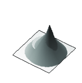
Figure 2: Regularized quasi-variational inequality with $\varepsilon=0.01$, $(Q^{h,\tau}_{A})$ approximation, simulation results for $h=0.02$, $\tau=0.01$. Left – the support surface $w_{0}$, the dashed line indicates the boundary of the support of $f$. Middle and Right – approximate sandpile surface, $W^{n}_{A}$, corresponding to $t=0.1$ and $t=0.2$, respectively.

The situation is similar for the quasi-variational inequality case, with only the evolving pile surface being approximated well using this method. In our second example, see Figure 2, we set $w_{0}=\max(0.5-|\underline{x}-\underline{x}_{0}|,0)$, where $\underline{x}_{0}=(0.3,0)$, for the square $\Omega=(-1,1)\times(-1,1)$. The source $f$ is uniform in its support $|\underline{x}|\leq 0.7$ with $\int_{\Omega}f(\underline{x},t)=1$ for all $t\geq 0$. For $h=0.02$ the generated mesh contained approximately 34,000 elements. Since the gradient constraint is now updated after each iteration of the splitting algorithm, existing theory does not guarantee its convergence. We found that, for the regularization parameter $\varepsilon=0.01$, good convergence of this algorithm is achieved for a smaller value of the augmented Lagrangian parameter $\rho$. In this example we chose $\rho=0.05$ with stopping criterion (5.1) and obtained the solution with $\tau=0.005$ and twenty time steps in 11 minutes of CPU time.

5.2 Approximation (Q${}^{h,\tau}_{B,r}$)

This approximation performed better in the variational inequality example from the previous section, recall Figure 1. Using the time step, $\tau=0.005$, and meshes, $h$=0.02 and 0.04, we obtained, for $t=0.1$, the pile surface with smaller relative errors in the $L^{1}$ norm; 0.1% and 0.6%, respectively. Furthermore, for this approximation the fluxes $Q^{n}_{B,r}$ also converged to the exact solution. Comparing the approximate and exact fluxes at the element centers we estimated the relative flux error in the $L^{1}$ norm. For the two meshes chosen these errors were, correspondingly, 2.8% and 5.2%.

Choosing a different initial support, $w_{0}(\underline{x})=\max(0.4-|\underline{x}|,0)$, and keeping the same source $f$ and domain $\Omega$ from the variational inequality example, we arrive at a quasi-variational inequality problem that can be solved analytically for the unregularized $M(\cdot)$. Being discharged from the source, sand now pours down the steep conical part of the support surface and forms a pile around this cone. The volume of the pile is $t$ and its surface $w(|\underline{x}|,t)=k_{0}\,(R_{2}(t)-|\underline{x}|)$ for $|\underline{x}|\in[R_{1}(t),R_{2}(t)]$, see Figure 3. Using simple geometric arguments, we first find the two variables, $R_{1}(t)$ and $R_{2}(t)$, determining this surface from the equations

$$t=\frac{\pi}{3}\left[(R_{2}^{3}-R_{1}^{3})\,k_{0}-(0.4^{3}-R_{1}^{3})\right]\quad\mbox{and}\quad R_{2}=R_{1}+\frac{1}{k_{0}}(0.4-R_{1})\,.$$

We then find the flux using the balance equation (5.3).

We solved the problem numerically, see Figure 4, with the regularization parameter $\varepsilon=0.005$ and estimated the errors of $W_{B,r}^{n}$ and $\underline{Q}_{B,r}^{n}$ at $t=0.1$ using the analytical solution. As could be expected, the smaller the value of $\varepsilon$, the more difficult it is to obtain convergence of the iterations (4.12) in the quasi-variational inequality case. We were, however, able to achieve convergence of these iterations by decreasing the time step $\tau$. For the stated value of $\varepsilon$, we chose $\tau=0.0005$ yielding 200 time steps on the time interval $[0,0.1]$ for two different meshes. For a mesh generated with $h=0.04$ the relative errors in the $L^{1}$ norm were 0.6% for the pile surface and 5% for the surface flux. For a finer mesh, $h=0.02$, the corresponding errors were 0.1% and 2%. These results confirm the validity of our regularization, $M_{\varepsilon}(\cdot)$, of $M(\cdot)$.

\psfrag{Y}{$y$}\psfrag{f}{$f$}\psfrag{R1}{{$R_{1}(t)$}}\psfrag{R2}{$R_{2}(t)$}\psfrag{R}{$|\underline{x}|$}\psfrag{0.4}{0.4}\psfrag{0}{0}\includegraphics[width=284.52756pt,height=142.26378pt]{qvi_ill.eps}

Figure 3: Sandpile, yellow region, forming upon the support platform with a steep cone.

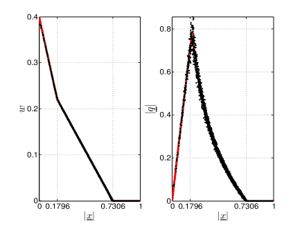
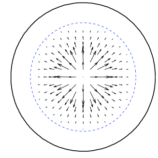
Figure 4: Regularized quasi-variational inequality with $\varepsilon=0.005$, $(Q^{h,\tau}_{B})$ approximation, simulation results for $h=0.04$, $\tau=0.0005$ and $t=0.1$. Left – exact surface $w(|\underline{x}|,t)$ (red line) and its approximation $W^{n}_{B,r}$ in the elements (black dots). Middle – exact flux modulus $|\underline{q}(|\underline{x}|,t)|$ (red line) and its approximation $|\underline{Q}^{n}_{B,r}|$ at the element centers (black dots). Right – the $\underline{Q}^{n}_{B,r}$ vector field, where the dashed line indicates the exact pile boundary.

We solved again, now using $(Q^{h,\tau}_{B,r})$, the quasi-variational problem considered in Figure 2 above, using the same mesh, time step, and the value of regularization parameter. Now we were able to find good approximations, not only to the pile surface but the surface flux as well, see Figure 5; and the computation time was about the same. We note that as the surface $W^{n}_{B,r}$ touches the support boundary $\partial\Omega$ at some time in the interval $(0.1,0.2)$ sand flows out of the system, which can be seen from the flux $Q^{n}_{B,r}$.

 

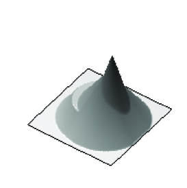
Figure 5: Regularized quasi-variational inequality with $\varepsilon=0.01$ as in Figure 2, $(Q^{h,\tau}_{B})$ approximation, simulation results for $h=0.02$, $\tau=0.01$ and $t=0.2$. Left – the calculated surface $W^{n}_{B,r}$. Middle – the flux modulus $|\underline{Q}^{n}_{B,r}|$ at the element centers. Right – the $\underline{Q}^{n}_{B,r}$ vector field and level contours of $W^{n}_{B,r}$.

In our last example $\Omega=(-1,1)\times(-1,1)$ and $w_{0}=\min(\max(|x_{1}|-0.9,|x_{2}|-0.9),0)$ is the surface of an inverted pyramid supplemented, to satisfy the no-influx condition (1.10), by a narrow horizontal margin. The uniform source is $f(\underline{x},t)\equiv 0.25$. Sand, discharged from the source, flows down the pyramid faces until it reaches a pyramid edge; then it pours down along the edge and forms a pile above the apex of the inverted pyramid, see Figure 6. Our numerical solution clearly shows the singularity of the edge fluxes.

Figure 6: Regularized quasi-variational inequality with $\varepsilon=0.02$, $(Q^{h,\tau}_{B})$ approximation, simulation results for $h=0.02$, $\tau=0.0025$ and $t=0.075$. Left – initial surface $w_{0}$ (blue lines) and the approximate surface $W^{n}_{B,r}$ in the elements (grey surface). Middle – the flux modulus $|\underline{Q}^{n}_{B,r}|$ at the element centers. Right – $\underline{Q}^{n}_{B,r}$ vector field and levels of $W^{n}_{B,r}$.