Integrability on the Master Space

Abstract

It has been recently shown that every SCFT living on D3 branes at a toric Calabi-Yau singularity surprisingly also describes a complete integrable system. In this paper we use the Master Space as a bridge between the integrable system and the underlying field theory and we reinterpret the Poisson manifold of the integrable system in term of the geometry of the field theory moduli space.

1 Introduction

Recently the AdS/CFT correspondence has been successfully applied to many fields of research both in physics and in mathematics. One of the most understood and investigated realization of the correspondence concerns the relation between type IIB supergravity on AdS${}_{5}\times Y$ and four dimensional SCFT describing the low energy dynamics of a stack of N D$3$ branes probing the tip of the Calabi-Yau (CY) cone $\mathcal{X}$=C(Y) over the five dimensional Sasaki Einstein manifold $Y$. When the CY singularity is toric, namely it has at least $U(1)^{3}$ isometry, many tools have been developed to deeply study the correspondence (see Kennaway:2007tq for reivew).

Indeed in this specific case the SCFT living on a stack of N D$3$ branes is a specific type of quiver gauge theory: it has $SU(N)^{g}$ gauge group and matter fields in the bifundamental representation of the gauge group, that appear just two times in the superpotential, once with positive sign and once with negative sign. All the information of these SCFT can be encoded in a dual structure, a bipartite graph on a torus, called the brane tiling and it gives a relation between the SCFT and the statistical mechanics of this graph Hanany:2005ve ; Franco:2005rj ; Hanany:2005ss ; Feng:2005gw . The partition function of the brane tiling contains the informations regarding the mesonic moduli space of the toric quiver gauge theory, namely the $\mathcal{X}$ geometry itself, and the toric data can be encoded in a polyhedral cone called the 2d toric diagram. Thanks to these results the study of the moduli space of $\mathcal{N}=1$ SCFT has been related to the mathematical literature of graph theory, and the developments on one side could foster the developments on the other side.

Very recently a new exciting result has been reported in Goncharov:2011hp . It has indeed been observed that starting from the bipartite graph for the SCFT we have just described, one can construct a completely integrable system, in which the oriented loops of this graph are the dynamical variables. The Poisson manifold 2008InMat.175..223F associated to this system is the collection of bipartite diagrams (seeds) glued via Poisson cluster transformations. These transformations, also known as mutations, have been studied on quiver diagrams in 2007arXiv0704.0649D .

It is interesting to investigate if the Poisson manifold can be analyzed with the field theory language of toric $\mathcal{N}=1$ SCFT. The study of the physical implication of the integrability of the bipartite graph in field theory started in Franco:2011sz ; Eager:2011dp ; Eager:2011ns . In Franco:2011sz the connection between the brane tiling, the quantum Teichmuller theory and the Poisson structure was investigated. Then in Eager:2011dp the Poisson manifold was studied in the language of quiver gauge theory and interesting connections with five dimensional $\mathcal{N}=1$ theories were made. Then in Eager:2011ns a connection with cluster algebra and flavored quiver models was proposed.

In this paper we want to show that the coherent component of the Master Space ${}^{{\rm Irr}}\!{\cal F}^{\flat}_{~{}}$ provides also a geometrical description of the integrable system introduced in Goncharov:2011hp . In Forcella:2008bb ${}^{{\rm Irr}}\!{\cal F}^{\flat}_{~{}}$ was introduced as the natural variety to describe the full moduli space of the $\mathcal{N}=1$ SCFT and the spectrum of supersymmetric gauge invariant operators for any number N of D3 branes. The master space $\mathcal{F}^{\flat}$ is the full moduli space of one D$3$ brane probing the CY cone and it is the union of the baryonic and mesonic moduli spaces. $\mathcal{F}^{\flat}$ is a reducible $g+2$ dimensional algebraic variety, and its largest irreducible component is ${}^{{\rm Irr}}\!{\cal F}^{\flat}_{~{}}$ that it has been shown in Forcella:2008bb to be a $g+2$ dimensional toric CY manifold. ${}^{{\rm Irr}}\!{\cal F}^{\flat}_{~{}}$ is a toric variety and it has a natural action of the $U(1)^{g+2}$ symmetries coming from the field theory global $U(1)$ symmetries: three mesonic and $g-1$ baryonic. Since it is a conical toric variety it can be represented as an integer $g+2$ dimensional fan of vectors in the $\mathbb{Z}^{g+2}$ lattice. Moreover, because ${}^{{\rm Irr}}\!{\cal F}^{\flat}_{~{}}$ is CY, the vectors describing the fan are coplanar. The crucial connection between this variety and the Poisson manifold consists in relating the Poisson brackets among the loops of the bipartite graph Goncharov:2011hp with an induced algebra among the $U(1)$ charges encoded in ${}^{{\rm Irr}}\!{\cal F}^{\flat}_{~{}}$, and in identifying the chemical potentials of these charges as the natural canonical coordinates on a patch of the Poisson manifold. The adjacency matrix of the quiver theory will be the link between the Poisson algebra on the loops and the Poisson algebra on the $U(1)$ charges, while the vectors defining ${}^{{\rm Irr}}\!{\cal F}^{\flat}_{~{}}$ will provide the map between the loop variables of the system and the local coordinates given by the chemical potentials. On every patch the Hamiltonians and the Casimir operators will be naturally expressed in terms of these local coordinates and they will be crucial to construct the full Poisson manifold. Indeed the different patches should be related by canonical transformations obtained mapping the Casimir operators, the Hamiltonians and their flows between two ${}^{{\rm Irr}}\!{\cal F}^{\flat}_{~{}}$ of Seiberg dual phases associated to the same SCFT.

In section 2 we review some useful material for the study of four dimensional toric quiver gauge theories, and the description of the moduli space in terms of dimer models. In 2.1 we introduce the master space and its irreducible component ${}^{{\rm Irr}}\!{\cal F}^{\flat}_{~{}}$. In section 3 we review the cluster integrable dimer model derived in Goncharov:2011hp . We discuss the Poisson structure, the Casimir operators and the Hamiltonians in terms of loops on the dimer. In section 4 we illustrate the main result of the paper. We explain the relation among the toric diagram describing the master space and the Poisson structure on the dimer model. We give the detailed dictionary among the coordinates used in Goncharov:2011hp and the $U(1)$ global charges of ${}^{{\rm Irr}}\!{\cal F}^{\flat}_{~{}}$. In 4.1 we define the explicit algorithm to compute the Poisson structure among the charges and we define the Hamiltonians and the Casimir operators in our coordinates. In section 5 we study some detailed examples. We use the cone over the dP₀ surface as an illustrative example to fix the notation and the general procedure. Then we study the two Seiberg dual phases of the cone over $\mathbb{F}_{0}$. We then move to the cases with more Hamiltonians: $Y^{30}$ and $Y^{40}$. In section 6 we analyze in more detail the relation between Seiberg dualities and the canonical map between the ${}^{{\rm Irr}}\!{\cal F}^{\flat}_{~{}}$ of the two phases of $\mathbb{F}_{0}$. In section 7 we conclude and discuss some interesting future directions.

In appendix A we review the derivation of the antisymmetric structure of Goncharov:2011hp as an intersection pairing among the cycles on the tiling. Then in appendix B we give some details about Seiberg duality as explained in Goncharov:2011hp . In the last appendix C we explicitly show the perfect matchings of $Y^{30}$ and $Y^{40}$.

2 Toric quiver gauge theories and dimer models

In this section we briefly review the topic of superconformal $\mathcal{N}=1$ four dimensional quiver gauge theories describing a stack of $N$ D$3$ branes probing toric CY₃ singularities. To simplify the discussion we make use of an example, which will be useful for the rest of the paper. The example we are referring to is the $\mathbb{Z}_{3}$ chiral orbifold of $\mathcal{N}=4$ SYM, also known as the cone over the dP₀ singularity.

The quiver is a connected two dimensional finite graph with nodes, which encodes all the information about the field content and the gauge symmetries of the theory. The nodes represent the $SU(N)$ gauge groups while the oriented arrows connecting the nodes represent the $\mathcal{N}=1$ chiral multiplets. The orientation of the arrows defines the representation of the field under the gauge groups. The incoming arrows with respect of the $i-th$ node are associated with the fundamental representation under $SU(N)_{i}$ while the outcoming arrows are associated to the antifundamental representation. Every endpoint of each arrow ends on a node, and the only admissible representation are adjoint and bifundamental. For instance in the case of dP₀ the quiver is given in the Figure 1 and it is associated to a product of three $SU(N)$ gauge groups with three chiral bifundamental fields connecting each pair of nodes, $X_{12}^{(i)}$, $X_{23}^{(i)}$ and $X_{31}^{(i)}$, with $i=1,2,3$.

Useful tools to describe the quiver are the oriented incidence and the adjacency matrices. For a quiver with $g$ vertices (gauge groups) and $\varepsilon$ oriented edges (bifundamental fields), the oriented incidence matrix $d$ is an $g\times\varepsilon$ matrix such that the $(\mathbb{g},e)$-th entry is $1$ (or $-1$) if the edge labelled $e$ is ingoing (or outgoing) to the $\mathbb{g}$-th vertex and zero otherwise. The adjoint fields always contribute as zero.

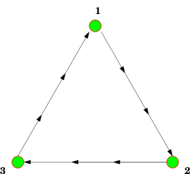
Figure 1: Quiver diagram for dP₀

Here for $dP_{0}$ the oriented incidence matrix is

$$d=\left(\begin{array}[]{c||ccccccccc}&X_{12}^{(1)}&X_{12}^{(2)}&X_{12}^{(3)}&X_{23}^{(1)}&X_{23}^{(2)}&X_{23}^{(3)}&X_{31}^{(1)}&X_{31}^{(2)}&X_{31}^{(3)}\\ \hline\cr 1&1&1&1&0&0&0&-1&-1&-1\\ 2&-1&-1&-1&1&1&1&0&0&0\\ 3&0&0&0&-1&-1&-1&1&1&1\end{array}\right)$$ (1)

From the incidence matrix one can define the antisymmetric oriented adjacency matrix as $a=d|d^{T}|$. This is a quadratic $g\times g$ matrix such that the $(\mathbb{g}_{i},\mathbb{g}_{j})$-th entry is the number of arrows from $\mathbb{g}_{i}$ to $\mathbb{g}_{j}$, counted with their orientation where $\mathbb{g}_{i}$ and $\mathbb{g}_{j}$ are vertices. For $dP_{0}$ it is

$$a=\left(\begin{array}[]{ccc}0&3&-3\\ -3&0&3\\ 3&-3&0\\ \end{array}\right)$$ (2)

Note that the row and columns of the adjacency matrix always sum to zero for anomaly cancellation.

The quiver diagram, together with a superpotential $W$, completely defines the gauge theory describing the D$3$ branes probing the toric CY. The superpotential is a function of the chiral fields associated to the edges and in the toric case it has a constrained structure. Every field appears precisely only twice in $W$ and with opposite sign. The information about the superpotential can be directly added to the quiver diagram by defining a periodic graph, called the planar quiver. In this diagram the superpotential terms become the boundary of oriented polygons (plaquettes). The plaquettes are glued together along the fields that belong to both the superpotential terms. The orientation of the plaquettes determines the signs of the superpotential terms.

This geometrical structure is very useful because its dual graph is a polygonal tiling of a torus, called the brane tiling Franco:2005rj . This graph is defined from the periodic quiver by replacing each faces with a vertex. Then edges separating two adjacent faces are replaced by dual edges and the vertices are replaced by faces, delimited by the dual edges.

This graph is bipartite (every vertex is black or white) and this assignment is defined by the orientation of the plaquettes. The vertices of the dimer represent the superpotential interactions, while the faces are related to the gauge groups.

In the case of dP₀ the periodic quiver and the bipartite diagram are shown in Figure 2.

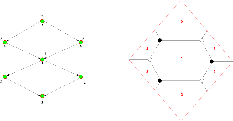
Figure 2: Periodic quiver and bipartite diagram for dP₀

The superpotential can be easily read from these Figure and it is

$$W=\epsilon_{ijk}X_{12}^{(i)}X_{23}^{(j)}X_{31}^{(k)}$$ (3)

On this graph one can identify different sets of marked edges (dimers) connecting the black and white nodes. A perfect matching is a collection of dimers chosen so that every vertex of the graph is covered by exactly one dimer. The bipartite graph together with its perfect matchings defines the dimer model. In this case we can identify the perfect matchings of dP₀ as in the Figure 3.

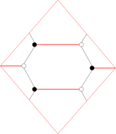
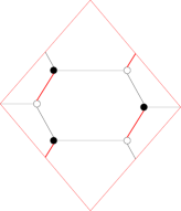
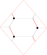
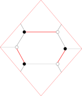
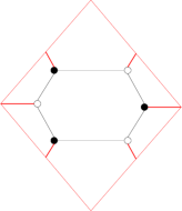
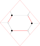
Figure 3: Perfect matchings for dP₀: in the first line we represented the external perfect matchings, $\pi_{1}$, $\pi_{2}$ and $\pi_{3}$ while in the second line we represented the internal three perfect matchings, $\sigma_{1}$, $\sigma_{2}$ and $\sigma_{3}$

The perfect matchings can be encoded in an $\varepsilon\times c$ matrix, where $\varepsilon$ represents the number of fields and $c$ is an index running on the perfect matchings. In this case we have

$$P=\left(\begin{array}[]{c|cccccc}&\pi_{1}&\pi_{2}&\pi_{3}&\sigma_{1}&\sigma_{2}&\sigma_{3}\\ \hline\cr X_{12}^{(1)}&1&0&0&1&0&0\\ X_{12}^{(2)}&0&1&0&1&0&0\\ X_{12}^{(3)}&0&0&1&1&0&0\\ X_{23}^{(1)}&1&0&0&0&1&0\\ X_{23}^{(2)}&0&1&0&0&1&0\\ X_{23}^{(3)}&0&0&1&0&1&0\\ X_{31}^{(1)}&1&0&0&0&0&1\\ X_{31}^{(2)}&0&1&0&0&0&1\\ X_{31}^{(3)}&0&0&1&0&0&1\end{array}\right)$$ (4)

Finally, on the dimer model one can define a partition function as the determinant of a matrix, called the Kasteleyn matrix Kasteleyn . This is a weighted signed adjacency matrix of the graph in which the rows and the columns represent the black and white nodes respectively. The $ij$-th elements of the matrix are the fields connecting the pairs of black and white nodes associated to $i$ and $j$. Each element is then wighted by the intersection number of these fields with the homology classes $(1,0)$ and $(0,1)$ of $\gamma_{w}$ and $\gamma_{z}$ winding cycles of the torus. In this case we have

$$\text{Kas}=\left(\begin{array}[]{ccc}X_{12}^{(1)}&X_{31}^{(3)}&X_{23}^{(2)}wz\\ X_{23}^{(3)}w^{-1}&X_{12}^{(2)}&X_{31}^{(3)}\\ X_{31}^{(2)}&X_{23}^{(1)}z^{-1}&X_{12}^{(3)}\end{array}\right)$$ (5)

The permanent of this matrix counts the perfect matchings of the brane tiling and their homology. In the case of dP₀ the permanent is

$$\text{Perm}(\text{Kas}) = X_{12}^{(1)}X_{12}^{(2)}X_{12}^{(3)}+X_{23}^{(1)}X_{23}^{(2)}X_{23}^{(3)}+X_{31}^{(1)}X_{31}^{(2)}X_{31}^{(3)}$$ (6)

$$+ \frac{1}{z}X_{12}^{(1)}X_{23}^{(1)}X_{31}^{(1)}+wzX_{12}^{(2)}X_{23}^{(2)}X_{31}^{(2)}+\frac{1}{w}X_{12}^{(3)}X_{23}^{(3)}X_{31}^{(3)}$$

This is a polynomial in the $w$ and $z$ variables and one can associate a polyhedral on $\mathbb{Z}^{2}$ to this polynomial, the toric diagram Fulton . This rational polyhedral encodes the data of the conical toric Calabi-Yau and the information of the mesonic moduli space on the field theory side.

In this case the polynomial (6), once represented on $\mathbb{Z}^{2}$, has three external points with coordinates $(1,1)$, $(-1,0)$ and $(0,-1)$. There is also an internal point $(0,0)$ associated to the three perfect matchings without $w$ and $z$ dependence in (6). From now on we will refer to the perfect matching associated to the external points as external perfect matchings (denoted as $\pi$) while the ones associated to the internal points are internal perfect matchings (denoted as $\sigma$). For example in Figure 3 we distinguished the internal perfect matchings in the first line and the external ones in the second.

2.1 The master space

The moduli space of a supersymmetric field theory is the set of all the possible constant vacuum expectation values of the scalar gauge invariant operators of the theory that satisfy the zero energy condition. This variety contains a lot of information regarding the field theory and it is the solution of the zeros of the derivatives of the superpotential with respect to the elementary scalar fields (F-terms condition), modulo the action of the complexified gauge group. In Forcella:2008bb ; Butti:2007jv it was discovered that, in the particular case of N D3 branes at toric CY₃ singularities, the information of a peculiar branch of the moduli space for one brane, is enough to reconstruct the full moduli space of the theory for generic N. This branch is called the coherent component of the master space ${}^{{\rm Irr}}\!{\cal F}^{\flat}_{~{}}$, it is a $g+2$ dimensional CY and it can be obtained as the symplectic quotient implementation of the linear relations among the $c$ perfect matchings of the dimer model associated to $\mathcal{X}$. Indeed the $c$ perfect matchings $p_{i}$ of a specific brane tiling are not free but they satisfy a set of $c-g-2$ linear relations, and they can be thought as $c$ vectors $V_{p_{i}}$ in $\mathbb{Z}^{g+2}$ subjected to these relations

$$\sum_{i=1}^{c}Q_{i}^{s}V_{p_{i}}=0$$ (7)

with $s=1,...,c-g-2$. We can now assign a complex coordinate $x_{p_{i}}$ of $\mathbb{C}^{c}$ to every vector $V_{p_{i}}$ and obtain the coherent component of the master space ${}^{{\rm Irr}}\!{\cal F}^{\flat}_{~{}}$ as the symplectic quotient

$${}^{{\rm Irr}}\!{\cal F}^{\flat}_{~{}}=\mathbb{C}^{c}//Q^{s}$$

In the example of dP₀ the relation among the perfect matching is simply $\pi_{1}+\pi_{2}+\pi_{3}=\sigma_{1}+\sigma_{2}+\sigma_{3}$ as can be seen from the Figure 3. The master space is then

$$\mathbb{C}^{6}//\{-1,-1,-1,1,1,1\}\qquad$$ (8)

An explicit representation of this toric variety is a toric diagram in $g+2$ dimensions, modulo a $SL(g+2,\mathbb{Z})$ transformation. Here we have $g=3$ and the toric diagram is described by the matrix

$$T=\left(\begin{array}[]{cccccc}\pi_{1}&\pi_{2}&\pi_{3}&\sigma_{1}&\sigma_{2}&\sigma_{3}\\ \hline\cr 0&0&1&1&0&0\\ 0&0&1&0&1&0\\ 1&0&0&0&0&1\\ 0&1&0&0&0&1\\ 0&0&1&0&0&1\end{array}\right)$$ (9)

where we indicated the perfect matching associated to every column. An useful way to think about $T$ is that every raw of the matrix determines the $U(1)$ charge of every perfect matching. The $i$-th index of $T_{i,\rho}$ parameterizes one of the the global $g+2$ $U(1)$ charge while the $\rho$-th index runs over the perfect matchings.

3 Dimer models and integrable systems

In this section we review the results derived in Goncharov:2011hp , relating the dimer models to integrable systems.

3.1 Poisson manifold and Poisson structure

An integrable system is usually described on a Poisson manifold, i.e. a manifold with an antisymmetric Poisson structure $\{,\}$. A Poisson manifold is symplectic if the rank of the antisymmetric structure equals everywhere the dimension of the Poisson manifold, and the antisymmetric structure can be written locally in terms of canonical variables $\mathbf{q}$ and $\mathbf{p}$.

However, more generically, the Poisson structure can have lower rank over the Poisson manifold. In this case there exist some operators which commute with everything: the Casimir operators. By fixing the value of these operators one usually restrict to an even dimensional symplectic leaf. This even dimensional subspace inherits the anticommuting structure of the Poisson manifold, and here the rank of the operator $\{,\}$ is maximal. In these cases, given a $2I+d-1$ dimensional Poisson manifold, one can find local coordinates $(c_{1},\dots,c_{d-1},\mathbf{q}_{1},\dots,\mathbf{q}_{I},\mathbf{p}_{1},\dots,\mathbf{p}_{I})$ such that $(\mathbf{q}_{1},\dots,\mathbf{q}_{I},\mathbf{p}_{1},\dots,\mathbf{p}_{I})$ satisfy canonical Poisson brackets and $(c_{1},\dots,c_{d-1})$ commute with everything.

An integrable system on this manifold is defined by $I$ independent functions $H_{a}$ which are in involution. Then on every symplectic leaf one can operate a change of variables. The new variables are usually named action and angle variables. The action variables commute among each other and generate the dynamics of the angle variables.

In Goncharov:2011hp it was shown that a dimer model can be associated to a Poisson manifold. Closed oriented loops $\alpha_{i}$ on the dimer corresponds to functions on the Poisson manifold, and their Poisson brackets is given by

$$\{\alpha_{i},\alpha_{j}\}=\epsilon(\alpha_{i},\alpha_{j})\alpha_{i}\alpha_{j}$$ (10)

where $\epsilon(\alpha_{i},\alpha_{j})$ is an antisymmetric intersection index specified by the construction that we review in the appendix A. Observe that closed oriented loops on the dimer can be always obtained as difference of two perfect matchings.

A complete set of coordinates on a patch of the Poisson manifold is given by $w_{A}$ and $z_{1,2}$. The $w_{A}$ are the loops around the faces of the tiling, while $z_{1}$ and $z_{2}$ represent two paths around the torus with homology $(1,0)$ and $(0,1)$ respectively. We stress that in this basis the anticommuting structure among the trivially homological loops $w_{A}$ is

$$\{w_{A},w_{B}\}=a_{AB}w_{A}w_{B}$$ (11)

and it is simply specified by the adjacency matrix $a_{AB}$. Note that the product of the whole set of closed loops cover the torus and it becomes trivial, $w_{1}\cdot w_{2}\dots w_{g-1}\cdot w_{g}=1$. The Poisson manifold has then dimension $g+1$, where $g$ is the number of gauge groups in the corresponding gauge theory.

3.2 Hamiltonian and Casimir operators

The Casimir operators and the Hamiltonians which define the integrable system consist of cycles on the bipartite graph. These are specified as differences of perfect matchings, depending on their homologies. A straightforward way to describe these quantities appears after the toric diagram is considered. Indeed different points of the diagram are related to different homologies of the perfect matchings in the tiling (see the previous section for the procedure of finding the homology of each perfect matching). We label as $\pi_{k}$ the $d$ perfect matchings associated to external points in the toric diagram, and with $\sigma_{k_{a}}^{a}$ the $r$ perfect matchings associated to internal points in the toric diagram. The superscript $a$ defines the homology of each perfect matching (it is in 1-1 correspondence with the internal points of the toric diagram, counted without multiplicity) and it runs from $1$ to $I$. Every internal point has a degeneracy $M_{a}$, which depends on the detail of the bipartite diagram. The subscript $k_{a}$ runs from $1$ to $M_{a}$ such that the $\sum_{a=1}^{I}M_{a}=r$ and finally $d+r=c$.

We choose a reference perfect matching among the external ones, that we label as $\pi_{ref}$. The Casimir operators are the cycles obtained as differences of the other external perfect matchings with respect to the reference one. There are thus $d-1$ independent Casimir operators .

The Hamiltonians are composed by cycles built as differences of internal perfect matchings with the same homology minus the reference perfect matching. Precisely, there are $I$ Hamiltonians, one for each internal point with a defined homology $a$. Each Hamiltonian $H^{a}$ is made of a sum of cycles, i.e. a sum of functions on the Poisson manifold. These cycles are built as the difference of the perfect matchings associated to the internal point with homology $a$, minus the reference perfect matching. For instance, the Hamiltonian corresponding to the $\sigma_{k_{a}}^{a}$ perfect matchings is

$$H^{a}=\sum_{k_{a}=1}^{M_{a}}\left(\sigma_{k_{a}}^{a}-\pi_{\text{ref}}\right)$$ (12)

It was proven in Goncharov:2011hp that, with respect to the Poisson structure defined by (10), the Casimir operators have vanishing Poisson brackets with everything, i.e. with every closed loop on the dimer. Moreover, the Hamiltonians built as in (12) commute one each other, providing an algebraic integrable system.

In conclusion, given a tiling with $g$ faces, the toric diagram has $I$ internal points and $d$ external points. The relation among $g$, $d$ and $I$ is $g+1=d-1+2I$. This relation tell us that we are describing a $g+1$-dimensional Poisson manifold (there are $g+2$ variables, but one constraint among the faces) with $d-1$ Casimir operators ($d-1$ are the independent relation among the differences of $d$ external perfect matchings) and $2I$ phase space variables. There are $I$ commuting Hamiltonians and the system is classically (and quantum 2008InMat.175..223F ; Goncharov:2011hp ) integrable.

4 Integrability on the master space

In this section we illustrate the main result of the paper, the connection between the integrable dimer models and the moduli space of the associated $\mathcal{N}=1$ SCFT gauge theory, or more precisely the coherent component of the master space ${}^{{\rm Irr}}\!{\cal F}^{\flat}_{~{}}$.

By following Goncharov:2011hp , we would like to point out that the same set of vectors $V_{p_{i}}$ defining the master space of the $\mathcal{N}=1$ SCFT describes also a patch of an integrable Poisson manifold. The full Poisson manifold is obtained by gluing together the patches associated to the master spaces of the different Seiberg dual phases of the $\mathcal{N}=1$ SCFT associated to the same CY cone $\mathcal{X}$. We offer in such a way a ”partial toric” description of the integrable cluster Poisson manifold.

Let us first analyze a patch. Because ${}^{{\rm Irr}}\!{\cal F}^{\flat}_{~{}}$ is a CY_g+2 the $c$ vectors $V_{p_{i}}$ lie on a $g+1$ dimensional hyperplane Forcella:2008bb and the set of differences of perfect matchings is a convex $g+1$ dimensional polytope $\Omega$ in $\mathbb{Z}^{g+2}$. ${}^{{\rm Irr}}\!{\cal F}^{\flat}_{~{}}$ has a natural projection to $\mathcal{X}$ obtained by disregarding the baryonic directions inside $\mathbb{Z}^{g+2}$: ${}^{{\rm Irr}}\!{\cal F}^{\flat}_{~{}}\rightarrow\mathcal{X}$. This projection allows to divide the $p_{i}$ in the external perfect matchings $\pi_{k}$, $j=1,...,d$, the ones that are mapped to the boundary of the 2d toric diagram of $\mathcal{X}$, and the internal perfect matchings $\sigma^{a}_{k_{a}}$, $k_{a}=1,...,M_{a}$, the ones that are mapped inside the 2d toric diagram, where $a=1,...,I$ labels the internal points of the toric diagram and $\sum M_{a}=c-d$. Moreover, thanks to the algorithm Hanany:2005ss , it is possible to obtain the adjacency matrix $a_{AB}$, $A,B=1,...,g$, from the $\pi_{k}$ for the various Seiberg dual phases.

We can now consider the $g+1$ dimensional cone defined by the $c-1$ vectors $V_{\delta p}$ obtained by subtracting to all the perfect matching vectors an arbitrary chosen external reference perfect matching vector $V_{\pi^{ref}}$. The $\delta p_{\rho}=p_{\rho}-\pi^{ext}$ are a set of $c-1$ cycles on the tiling. To every vector $V_{\delta p}$ we can now associate a local function:

$$f[V_{\delta p_{\rho}}]=e^{\sum_{m=1}^{g+1}x_{m}V^{m}_{\delta p_{\rho}}}$$ (13)

where $V^{m}_{\delta p_{\rho}}$ is the $m$-th coordinate associated to the $V_{\delta p_{\rho}}$ vector inside $\mathbb{Z}^{g+1}$, and $x_{m}$ is the associated chemical potential, one for every direction inside $\mathbb{Z}^{g+1}$. We would like to interpret the chemical potentials $x_{m}$ as a set of local coordinates inside a patch of an integrable Poisson manifold.

Given the matrix $a_{AB}$ there is a standard way to obtain the Poisson structure $J_{mn}$ on the local $x_{m}$ coordinates. Indeed the $a_{AB}$ is the natural Poisson structure Goncharov:2011hp on a particular subset of vectors in $\Omega$ called $V_{w_{A}}$. Actually there are $g$ different $w_{A}$ but they are constrained by $\prod w_{A}=1$, so there are only $g-1$ independent vectors $V_{w_{A}}$. The $w_{A}$ are a basis of zero homotopy cycles on the tiling: they are the closed loops around the $A$-th face of the tiling and they are obtained subtracting two internal perfect matchings belonging to the same internal point of the 2d toric diagram: $w_{A}=\sigma^{a}_{k_{a}}-\sigma^{a}_{k^{\prime}_{a}}$. As vectors they are a basis in the space of anomalous and non anomalous baryonic charges and they are uncharged under the two mesonic directions. To complete the local basis of charges one has to add the two cycles $z_{1}$ and $z_{2}$ on the tiling that have respectively homotopy (1,0) and (0,1) along the two torus directions, and they are associated to the vectors $V_{z_{1}}$, $V_{z_{2}}$ inside $\Omega$ charged under the mesonic symmetries. The Poisson brackets among the $V_{w_{A}}$ is defined as:

$$\{f[V_{w_{A}}],f[V_{w_{B}}]\}=a_{AB}f[V_{w_{A}}]f[V_{w_{B}}]=\sum_{mn}\partial_{x_{m}}f[V_{w_{A}}]\partial_{x_{n}}f[V_{w_{B}}]J_{mn}$$ (14)

The matrix $a_{AB}$ has rank $2I$, equal to the number of anomalous charges in the SCFT. Indeed it distinguishes the anomalous from the non anomalous baryonic symmetries and it can be put in the natural block form: $J_{g+1}=0_{d-1}\bigoplus J_{2I}$. The $d-1$ null part of the matrix is related to the non anomalous charges, while the $J_{2I}$ acts also on the anomalous charges and can be brought in the canonical form $J_{2I}=((0,\mathbb{I}_{I}),(-\mathbb{I}_{I},0))$. The chemical potentials for the non anomalous charges are coordinates associated to the Casimir operators, $c_{e}$, with $e=1,\dots,d-1$ while the chemical potential for the anomalous charges are the generalized coordinates $\overrightarrow{\mathbf{q}}$, and conjugate momenta $\overrightarrow{\mathbf{p}}$, and together they are local coordinates of a Poisson manifold.

Because the non anomalous charges are defined in toric geometry by the zero locus of the coordinates $x_{\pi_{k}}$ associated to the external perfect matchings, the $d-1$ functions that define the symplectic leaves of the manifolds can be identified with $f[V_{\delta\pi_{e}}]$. We have right now two interesting sets of $g+1$ vectors: $\mathcal{B}^{1}=\{V_{w_{A}},V_{z_{1}},V_{z_{2}}\}$ and $\mathcal{B}^{2}=\{V_{\delta\pi_{e}},V_{\delta\sigma_{\tilde{m}}}\}$, where the $V_{\delta\sigma_{\tilde{m}}}$, with $\tilde{m}=1,...,2I$, are a set of vectors perpendicular to $V_{\delta\pi_{e}}$ that form a basis of the anomalous charges inside $\mathbb{Z}^{g+1}$. Because every Poisson manifold admits a local set of coordinates given by the Casimir operators, the positions and conjugate momenta WEINSTEIN , there should exist a change of coordinates from $\mathcal{B}^{1}$ to $\mathcal{B}^{2}$. The existence of this transformation is assured by the CY condition of the master space. Indeed, the $\mathcal{B}^{1}$ and $\mathcal{B}^{2}$ are subtraction of different perfect matchings in $\mathbb{Z}^{g+2}$ and they both live in a $g+1$ dimensional hyperplane. The CY condition assure that all the perfect matchings live on the same $g+1$ dimensional hyperplane implying that the two hyperplanes of $\mathcal{B}^{1}$ and $\mathcal{B}^{2}$ are the same, and the existence of a linear transformation $\mathbb{M}$ between the two: $\mathcal{B}^{2}_{i}=\mathbb{M}_{ij}\mathcal{B}^{1}_{j}$.

The relation between $\mathcal{B}^{1}$ and $\mathcal{B}^{2}$ corresponds to a linear map among the vectors $V_{\delta p}$ inside $\Omega$. The vectors $V_{\delta p}$ are a set that generates all the possible subtractions of perfect matchings and they look the natural variables to describe the completely integrable Hamiltonian dynamics of the closed cycles of the tilings. We characterize the local patch of this completely integrable system as follows: to each vector $V_{\delta p_{i}}$ in $\Omega$ we associate a coordinate $y_{\delta p_{i}}$, and to the linear relations (7) we associate the algebraic constraints:

$$\prod_{i=1}^{c-1}y_{\delta p_{i}}^{Q_{i}^{s}}=1$$ (15)

which can be locally solved by the functions $f[V_{\delta p_{i}}]$ defined above. The open dense subspace over which this algebraic intersection can be solved in term of the local coordinates $x_{m}$ is one patch of the Poisson manifold and (15) are rational transformations among local coordinates of this patch. The dimension of the Poisson manifold is $g+1$. $y_{\delta\pi_{e}}$ are the $d-1$ Casimir operators, they are the level functions of the symplectic foliation and they are associated to the non anomalous global symmetries. The symplectic leaf is $2I$ dimensional, where $2I$ corresponds to the number of anomalous symmetries of the field theory. There are $I$ Hamiltonians and $I$ associated flow vectors, given by linear functions of the $y_{\delta p_{i}}$ coordinates:

$$H^{a}=\sum_{k_{a}=1}^{M_{a}}y_{\delta\sigma^{a}_{k_{a}}}\hbox{ }\hbox{ , }\hbox{ }\{H^{a},\hbox{ }\}=\sum_{k_{a}=1}^{M_{a}}\sum_{m,n}J_{mn}V^{m}_{\delta\sigma^{a}_{k_{a}}}y_{\delta\sigma^{a}_{k_{a}}}\partial_{x_{n}}$$ (16)

for $a=1,...,I$ and $k_{a}$ running over the number of internal perfect matchings associated to the same internal point of the toric diagram of $\mathcal{X}$. In the paper, we will show, example by example, that the $I$ Hamiltonians $H^{a}$ are in involution: $\{H^{a},H^{b}\}=0$, with respect to the $J_{2I}$ symplectic structure, and, as was proven in Goncharov:2011hp , the system is integrable.

In Goncharov:2011hp it is shown that the full Poisson manifold can be obtained by gluing together, with (cluster) Poisson transformations, the various patches associated to the closed loops in different Seiberg dual dimer model realizations of the SCFT living at $\mathcal{X}$. Indeed it is well known that to every $\mathcal{X}$ are associated different SCFT that are related by Seiberg duality (SD) transformations Feng:2000mi ; Beasley:2001zp ; Feng:2001bn . The ${}^{{\rm Irr}}\!{\cal F}^{\flat}_{~{}}$ for every SD phase is in general a different algebraic variety Forcella:2008ng . Following Goncharov:2011hp we would like to argue that the various patches of the Poisson manifold, obtained from the master space with the procedure we have just explained, can be glued together, along open dense subsets, with transition functions that are non toric symplectic morphisms on the symplectic leaves and toric transformations on the Casimir operators. Here we give some rules for the gluing procedure and in section 6 we check them using the $\mathbb{F}_{0}$ example and the procedure discussed in Goncharov:2011hp .

The ${}^{{\rm Irr}}\!{\cal F}^{\flat}_{~{}}$ of different SD phases are not isomorphic toric varieties Forcella:2008ng , however the non anomalous charges of the SD phases can be mapped among themselves. Indeed there exist a linear transformation that maps the $d-1$ external perfect matchings vectors $V_{\delta\pi_{e}}$ of one phase to the $d-1$ external perfect matchings vectors $V_{\delta\pi^{S.d.}_{e}}$ of the dual Seiberg phase, and it can be translated into a rational map between local coordinates of two patches in the usual toric way:

$$\sum_{e=1}^{d-1}D_{e}^{k}V_{\delta\pi_{e}}-\sum_{e=1}^{d-1}S^{k}_{e}V_{\delta\pi^{S.d.}_{e}}=0\hbox{ }\rightarrow\hbox{ }\prod_{e=1}^{d-1}y^{D_{e}^{k}}_{\delta\pi_{e}}=\prod_{e=1}^{d-1}(y_{\delta\pi_{e}^{S.d.}})^{S_{e}^{k}}$$ (17)

We will see indeed that the map among the Casimir operators of the system is a linear map on the chemical potentials for the non anomalous charges. The map between the symplectic leaves is obtained by mapping among themselves the SD Hamiltonians associated to the same internal point in the 2d toric diagram and the associated Hamiltonian flows:

$$H^{a}=H^{a}_{S.d},\hbox{ }\hbox{ }\{H^{a},...\}=\{H^{a}_{S.d},\hbox{ }\}_{S.d.}$$ (18)

This second transformation on the leaves of the Poisson manifold breaks the toricity of the map (it is not of the form monomial equal to monomial) and it translates, as we will see, in a non linear map among the canonical coordinates. More explicitly it can be written as:

$$\sum_{k_{a}}y_{\delta\sigma^{a}_{k_{a}}}=\sum_{k}y^{S.d.}_{\delta\sigma^{a}_{k_{a}}}\hbox{ }\hbox{ , }\hbox{ }\sum_{m,k_{a}}J_{mn}V^{m}_{y_{\delta\sigma^{a}_{k_{a}}}}y_{\delta\sigma^{a}_{k_{a}}}=\sum_{m,s,k_{a}}J^{S.d}_{ms}\frac{\partial x_{n}}{\partial x^{S.d.}_{s}}V^{m}_{y^{S.d.}_{\delta\sigma^{a}_{k_{a}}}}y^{S.d.}_{\delta\sigma^{a}_{k_{a}}}$$ (19)

These transformations are a set of algebraic and differential equations, they are defined on open dense subsets of the Poisson patches and are by definition Poisson isomorphisms.

4.1 The computing algorithms

After we have stated the correspondence we have to provide a computing algorithm to obtain the explicit expression for the Poisson structure and the Hamiltonians of the integrable systems in terms of the vectors defining the master space.

The only quantities necessary to study the Poisson structure and thus the integrability of the dimer models are the adjacency matrix, the matrix T defined in 2.1 and the parametrization of the loops in terms of differences of perfect matchings. Another necessary information is the identification of the perfect matchings corresponding to external and to internal points in the matrix $T$. Moreover, to build the Hamiltonians, we should identify the set of perfect matchings which correspond to each internal point. This is always possible by performing an $SL(g+2,\mathbb{Z})$ transformation on this matrix such to isolate the $2d$ toric diagram on the first two rows. Then we can choose an order for the columns of $T$, i.e. the perfect matchings, such that the first $d$ corresponds to the external points of the toric diagram and the others are all internal points.

Note that, in this ordering of the perfect matching, by applying another $SL(g+2,\mathbb{Z})$ transformation on $T$ we can then have the first $d$ columns charged only under $d$ of the $g+2$ symmetries. This fact has a simple interpretation on the field theory side: the external points of the toric diagram are uncharged under the $2I=g+2-d$ anomalous symmetries. This is a signal that the Casimir operators, defined as differences of external perfect matching, are associated with a trivial (vanishing) antisymmetric structure, since the only non zero part of the antisymmetric structure comes from the anomalous $U(1)$’s. Anyway, in what follows we do not specify any particular basis for the $U(1)$ charges, i.e. for the rows of the matrix $T$, and we proceed in complete generality.

We now define the loop matrix $\delta T$ as follows: first we fix one of the external perfect matchings as a reference perfect matching and then we subtract the associated columns of $T$ to all of the other columns of $T$:

$$\delta T_{i,\rho}=T_{i,\rho}-T_{i,\text{rif}}$$ (20)

Without loose of generality from now on we fix ”rif$=1$”. To fix the notation we refer to the columns of the $\delta T_{i,\rho}$ matrix as $\delta T=(0_{1},\mathcal{E}_{e},\mathcal{I}_{l})$, where $l=1,\dots,r$ runs over the number of internal perfect matchings (counted with multiplicities), $e=1,\dots,d-1$ runs over the external perfect matchings minus one, and $\rho=1,\dots,c$ over all the perfect matchings. The vectors of the matrix $\delta T$ are associated to loops in the brane tiling.

The CY condition of the master space implies that the $g+2$ dimensional vectors $\mathcal{E}_{e}$ and $\mathcal{I}_{l}$ all lie on the same hyperplane of dimension $g+1$. We define the perpendicular vector to this hyperplane

$$v=Ker[(\delta T)^{T}]$$ (21)

and we build a basis in the $g+2$ dimensional vector space

$$B_{i,J}=(\mathcal{E},\text{Ker}[v,\mathcal{E}],v)\qquad J=1,\dots,g+2$$ (22)

where Ker$[v,\mathcal{E}]$ is the orthogonal space to the the subspace spanned by the vectors $v$ and $\mathcal{E}_{e}$ in the $g+2$ dimensional lattice. This basis represents a mapping between the space of the $g+2$ $U(1)$ charges and the $g+2$ dimensional vector space . We can invert this matrix in order to obtain the inverse map $(B^{-1})_{J,i}$.

Every loop on the dimer is a difference of two perfect matchings which are determined by their $U(1)$ charges. We can express the loop charges in the basis of $g+2$ vectors via the map $B^{-1}$. Note that since the loop is a difference of two perfect matchings this combination will never involve the vector $v$. For instance, consider a cycle $\alpha$ corresponding to the difference of two perfect matchings $p_{1}-p_{2}$, which are themselves columns of the matrix $T$. This difference is a vector in the $g+2$ dimensional vector space and it is orthogonal to the vector $v$. Hence it can be expressed uniquely on the basis (22) as

$$(p_{1}-p_{2})_{i}=B_{i,J}\alpha_{J}\qquad\alpha_{J}=B^{-1}_{J,i}(p_{1}-p_{2})_{i}$$ (23)

with coefficients $\alpha_{J}$. Note that because of the argument we have just explained, the coefficient $\alpha_{g+2}$ will always be $0$. The associated function on the $g+1$ dimensional Poisson manifold is then

$$f[\alpha]=e^{\sum_{m=1}^{g+1}x_{m}B^{-1}_{m,i}(p_{1}-p_{2})_{i}}$$ (24)

where now $m$ runs only up to $g+1$. This gives the explicit realization of the map (13) on this special basis of charges.

The other information that we need to extract the Poisson structure is the composition of the loops $w_{A}$ (with $A=1,\dots,g$) as differences of perfect matchings, i.e. of columns of $T$. Every loop $w_{i,A}$ is then associated to a vector in the $g+2$ dimensional vector space, which can be written in the basis of $g+1$ vectors (22), as just explained. We can encode the parametrization of the cycles $w_{A}$ on the $g+2$ charges in a matrix $A_{i,A}$. Then we can write the corresponding functions on the Poisson manifold as

$$f[w_{A}]=e^{x_{m}B^{-1}_{m,i}A_{i,A}}$$ (25)

The $g\times g+2$ matrix A has rank $g-1$ since the $w_{A}$ satisfy the constraint $\prod_{A}w_{A}=1$, which translate in the functions as $\prod_{A}f[w_{A}]=1$. It encodes all the necessary data about the $w_{A}$ loops.

The $x_{m}$ represents the local coordinates on the Poisson manifold. Given the ordering of the basis $B$, the local coordinates are already organized in Casimir and phase space variables as $x_{m}=(c_{1},\dots,c_{d-1},q_{1},\dots,q_{2I})$ . These coordinates are in correspondence with the $U(1)$ charges. The first $d-1$ elements are associated to global non anomalous $U(1)$ symmetries and the last $2I$ to the anomalous ones. The Poisson structure for these local coordinates is given by

$$\{x_{m},x_{n}\}=J_{mn}=\left(\begin{array}[]{cc}0&0\\ 0&\tilde{J}_{\widetilde{m}\widetilde{n}}\end{array}\right)$$ (26)

where the matrix $\tilde{J}$ has dimension $2I\times 2I$ and $\{q_{\widetilde{m}},q_{\widetilde{n}}\}=\tilde{J}_{\widetilde{m}\widetilde{n}}$ is the antisymmetric structure of the phase space variables, not necessarily canonical in this basis. The antisymmetric structure $J_{\widetilde{m}\widetilde{n}}$ can be obtained by imposing the Poisson brackets (11) among the $w_{A}$ loops. Indeed we can solve the following equations

$$a_{AB}=\frac{\{f[w_{A}],f[w_{B}]\}}{f[w_{A}]f[w_{B}]}=\{\sum_{m}x_{m}B^{-1}_{m,i}A_{i,A},\sum_{n}x_{n}B^{-1}_{n,i}A_{i,B}\}=\sum_{m,n}(B^{-1}_{m,i}A_{i,A})(B^{-1}_{n,i}A_{i,B})J_{mn}$$ (27)

where $a_{AB}$ is the adjacency matrix, finding the antisymmetric structure $\tilde{J}_{\widetilde{m}\widetilde{n}}$. Note that the matrix $B^{1}_{m,i}$ has rank $g+1$, the matrix $A$ has rank $g-1$, and the matrix $a_{AB}$ has rank $2I$. For every toric diagram the inequality $d-3=g-1-2I\geq 0$ is satisfied. Hence the matrix $\tilde{J}_{\widetilde{m}\widetilde{n}}$ has also rank $2I$.

With this procedure we have obtained an explicit mapping between cycles, i.e. differences of two perfect matchings, and functions of local coordinates on the Poisson manifold. Moreover we have extracted the Poisson structure for this coordinate system. One can check that, taken two arbitrary closed cycles on the dimer, our mapping and Poisson structure reproduce the antisymmetric intersection algebra based on (10).

4.2 Hamiltonians

Once the Poisson structure is known, we can define the Hamiltonians and study the integrability of the system. Consider an internal point with homology $a$, related to a set of perfect matchings $\sigma_{k_{a}}^{a}$, where $k_{a}=1,\dots,M_{a}$ and $M_{a}$ is the multiplicity of the $a$-th internal point. This set of perfect matchings correspond to a set of $M_{a}$ different cycles with the same homology. They correspond to columns in $\delta T$, and we label them as $\delta T_{i,k_{a}}$. Each of these elements is a vector in the basis of the $g+2$ charges which can be expressed in the basis (22) via $B^{-1}$. Each Hamiltonian function is computed by summing the cycles with the same homology $a$

$$H^{a}=\sum_{k_{a}=1}^{M_{a}}e^{x_{m}B^{-1}_{m,i}\delta T_{i,k_{a}}}$$ (28)

The commutation relation of two Hamiltonians is then given by

$$\{H^{a},H^{b}\}= = \{\sum_{k_{a}=1}^{M_{a}}e^{x_{m}B^{-1}_{m,i}\delta T_{i,k_{a}}},\sum_{k_{b}=1}^{M_{b}}e^{x_{m}B^{-1}_{m,i}\delta T_{i,k_{b}}}\}$$

$$= \sum_{k_{a},k_{b}}e^{x_{m}B^{-1}_{m,i}\delta T_{i,k_{a}}+x_{n}B^{-1}_{n,i}\delta\tilde{T}_{i,k_{b}}}\sum_{m,n=1}^{g+1}(B^{-1}_{m,i}\delta T_{i,k_{a}})(B^{-1}_{n,i}\delta T_{i,k_{b}})J_{mn}$$

5 Examples

In this section we exemplify the general procedure explained in the previous sections in a series of examples of increasing complexity. We perform the case of the chiral gauge theory associated to the $dP_{0}$ singularity introduced before. Then we describe the two phases of $\mathbb{F}_{0}$, which will be later used to discuss Seiberg duality. We then show two examples with multiple internal points $Y^{(3,0)}$ and $Y^{(4,0)}$ to explicitly check that the Hamiltonians are in involution.

5.1 Theories with one Hamiltonian

5.1.1 $dP_{0}$

We here study the quiver gauge theory and the dimer associated to $N$ D$3$-branes probing the cone over the zeroth del Pezzo surface $dP_{0}$. In the previous sections we used this theory to review the computation of the moduli space for $\mathcal{N}=1$ toric SCFT. Here we apply the algorithm explained in section 4.1 to obtain the Poisson structure and the Hamiltonian.

The $T$ matrix (9) encodes the charges of the $6$ perfect matchings under the $g+2=5$ $U(1)$ global symmetries of the theory. Note that we already order it such that the first three columns correspond to the three external perfect matchings. Our construction is invariant under $SL(g+2,\mathbb{Z})$ transformation. Thus, to render the final expressions simpler, we can transform the matrix $T$ to a more easy form by acting with an $SL(5,\mathbb{Z})$ transformation, we obtain

$$T=\left(\begin{array}[]{cccccc}\pi_{1}&\pi_{2}&\pi_{3}&\sigma_{1}&\sigma_{2}&\sigma_{3}\\ 1&0&0&0&0&1\\ 0&1&0&0&0&1\\ 0&0&1&0&0&1\\ 0&0&0&1&0&-1\\ 0&0&0&0&1&-1\end{array}\right)$$ (30)

The external perfect matchings are uncharged under two of the $U(1)$ symmetries, which are identified with the anomalous $U(1)$’s of the theory.

From now one we fix the first external perfect matching as the reference perfect matching, and the $\delta T$ matrix becomes

$$\delta T=\left(\begin{array}[]{cccccc}0&-1&-1&-1&-1&0\\ 0&1&0&0&0&1\\ 0&0&1&0&0&1\\ 0&0&0&1&0&-1\\ 0&0&0&0&1&-1\end{array}\right)$$ (31)

The last information we need to extract the Poisson structure is the structure of the $w_{A}$ loops associated to the faces in the dimer. We can identify the loops as the differences ratio of the $y$ variables defined in section 4. We have

$$w_{1}=\frac{y_{\delta\sigma_{3}}}{y_{\delta\sigma_{1}}},\quad w_{2}=\frac{y_{\delta\sigma_{1}}}{y_{\delta\sigma_{2}}},\quad w_{3}=\frac{y_{\delta\sigma_{2}}}{y_{\delta\sigma_{3}}}$$ (32)

Thus, the matrix $B$ (22) , its inverse and the matrix $A$ (25) are

$$B=\left(\begin{array}[]{ccccc}-1&-1&-1&-1&1\\ 1&0&-1&-1&1\\ 0&1&-1&-1&1\\ 0&0&0&3&1\\ 0&0&3&0&1\end{array}\right),\quad B^{-1}=-\frac{1}{15}\left(\begin{array}[]{ccccc}~{}~{}5&-10&~{}~{}5&~{}~{}0&~{}~{}0\\ ~{}~{}5&~{}~{}5&-10&~{}~{}0&~{}~{}0\\ ~{}~{}1&~{}~{}1&~{}~{}1&~{}~{}1&-4\\ ~{}~{}1&~{}~{}1&~{}~{}1&-4&~{}~{}1\\ -3&-3&-3&-3&-3\end{array}\right),\quad A=\left(\begin{array}[]{ccc}1&0&-1\\ 1&0&-1\\ 1&0&-1\\ -2&1&1\\ -1&-1&2\end{array}\right)$$ (33)

The last column of $B$, i.e. the vector $v=(1,1,1,1,1)$, identifies the orthogonal direction in the master space, and it is perpendicular to all the vectors in (31).

The CY condition of the master space guarantees that the charges of every closed loop in the dimer can be expressed as a linear combination of the first four columns of $B$ only. We then project out the orthogonal direction and associate to the four independent $U(1)$ charges the four local coordinates of the Poisson manifold, parametrized as

$$\{x_{m}\}=(c_{1},c_{2},q_{1},q_{2})$$ (34)

The ordering we have chosen for the matrix $B$ (see eq. (22)) implies that the first two coordinates $c_{i}$ are associated to Casimir operators, while $q_{1}$ and $q_{2}$ are the phase space variables. By solving the relations (27), we find the antisymmetric structure among these local coordinates as

$$\{c_{e},c_{f}\}=0,\quad\{c_{e},q_{\widetilde{n}}\}=\{q_{\widetilde{m}},c_{f}\}=0,\quad\{q_{\widetilde{m}},q_{\widetilde{n}}\}=-9\,\epsilon_{\widetilde{m}\widetilde{n}}$$ (35)

The $y$ variables are parametrized in terms of the $\{x_{m}\}=(c_{e},q_{\widetilde{m}})$ variables as

$$y_{s}=e^{x_{m}B^{-1}_{mi}\delta T_{is}}$$ (36)

where $s$ runs over the external and internal perfect matchings. Precisely $s=(1,\dots,6)\rightarrow(\pi_{1},\pi_{2},\pi_{3},\sigma_{1},\sigma_{2},\sigma_{3})$, and we have

$$B^{-1}\delta T=\left(\begin{array}[]{c|cccccc}&\pi_{1}&\pi_{2}&\pi_{3}&\sigma_{1}&\sigma_{2}&\sigma_{3}\\ \hline\cr c_{1}&0&1&0&\frac{1}{3}&\frac{1}{3}&\frac{1}{3}\\ c_{2}&0&0&1&\frac{1}{3}&\frac{1}{3}&\frac{1}{3}\\ q_{1}&0&0&0&0&\frac{1}{3}&-\frac{1}{3}\\ q_{2}&0&0&0&\frac{1}{3}&0&-\frac{1}{3}\\ \end{array}\right)$$ (37)

With this matrix we parameterize the $y_{i}$ as

$$y_{\delta\pi_{1}}=1,\quad\quad\quad\quad y_{\delta\pi_{2}}=e^{c_{1}},\quad\quad\quad\,\,\,y_{\delta\pi_{3}}=e^{c_{2}}\quad\quad\quad$$

$$y_{\delta\sigma_{1}}=e^{\frac{c_{1}+c_{2}+q_{2}}{3}},\quad y_{\delta\sigma_{2}}=e^{\frac{c_{1}+c_{2}+q_{1}}{3}},\quad y_{\delta\sigma_{3}}=e^{\frac{c_{1}+c_{2}-q_{1}-q_{2}}{3}}\quad$$ (38)

The only Hamiltonian associated with the single internal point is obtained with the procedure explained in section 4.2 and it is

$$H=y_{\delta\sigma_{1}}+y_{\delta\sigma_{2}}+y_{\delta\sigma_{3}}$$ (39)

Finally, by introducing the paths $z_{1}$ and $z_{2}$ as

$$z_{1}=\frac{y_{\delta\sigma_{3}}}{y_{\delta\pi_{3}}},\quad z_{2}=\frac{y_{\delta\pi_{2}}}{y_{\delta\sigma_{3}}}$$ (40)

we reconstruct the algebra of the $w_{A}$ and $z_{1}$ and $z_{2}$ defined in Goncharov:2011hp from the algebra of the $c_{i}$ and $q_{\tilde{m}}$. Indeed the cycles $w_{A},z_{1},z_{2}$ are associated to exponential functions of the local coordinates via the mapping (24) and, by knowing the antisymmetric structure (35), their Poisson bracket can be obtained. We have

$$\left(\begin{array}[]{c|c}\frac{\{w_{A},w_{B}\}}{w_{A}w_{B}}&\frac{\{w_{A},z_{t}\}}{w_{A}z_{t}}\\ \hline\cr\frac{\{z_{u},w_{B}\}}{z_{u}w_{B}}&\frac{\{z_{u},z_{t}\}}{z_{u}z_{t}}\end{array}\right)=\left(\begin{array}[]{ccccc}0&3&-3&1&-1\\ -3&0&3&-2&2\\ 3&-3&0&1&-1\\ -1&2&-1&0&0\\ 1&-2&1&0&0\end{array}\right)$$ (41)

as in Franco:2011sz , where here $u,t=1,2$.

5.1.2 $\mathbb{F}_{0}^{(I)}$

The quiver gauge theory describing a stack of $N$ D$3$ branes over the zero Hirzebruch surface is described by the superpotential

$$W=\epsilon_{ij}\epsilon_{lk}X_{12}^{(i)}X_{23}^{(l)}X_{34}^{(j)}X_{41}^{(k)}$$ (42)

The quiver, the brane tiling, the toric diagram and the adjacency matrix are specified in the Figure 4.

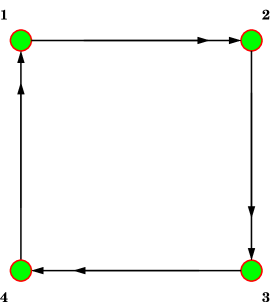
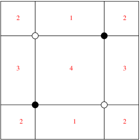
$a=\left(\begin{array}[]{cccc}0&2&0&-2\\ -2&0&2&0\\ 0&-2&0&2\\ 2&0&-2&0\end{array}\right)$

Figure 4: Quiver, brane tiling, toric diagram and adjacency matrix for $\mathbb{F}_{0}^{(I)}$

The four external points of the toric diagram are associated to the perfect matching in Figure 5 while the four degenerate internal points are given in Figure 6. They respect the relations

$$\pi_{2}+\pi_{4}=\sigma_{1}+\sigma_{4}\quad,\quad\pi_{1}+\pi_{3}=\sigma_{2}+\sigma_{3}$$ (43)

Figure 5: External perfect matchings of $\mathbb{F}_{0}^{(I)}$

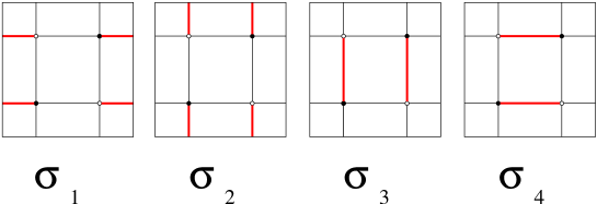
Figure 6: Internal perfect matchings of $\mathbb{F}_{0}^{(I)}$

The T matrix is then

$$T=\left(\begin{array}[]{cccccccc}\pi_{1}&\pi_{2}&\pi_{3}&\pi_{4}&\sigma_{1}&\sigma_{2}&\sigma_{3}&\sigma_{4}\\ 1&0&0&0&0&0&1&0\\ 0&1&0&0&0&0&0&1\\ 0&0&1&0&0&0&1&0\\ 0&0&0&1&0&0&0&1\\ 0&0&0&0&1&0&0&-1\\ 0&0&0&0&0&1&-1&0\end{array}\right)$$ (44)

We stress that our algorithm is manifestly $SL(g+2,\mathbb{Z})$ invariant and we are choosing this basis only for having more manageable expressions. From now one we fix the first external perfect matching as the reference one, and the $\delta T$ matrix is

$$\delta T=\left(\begin{array}[]{cccccccc}0&-1&-1&-1&-1&-1&0&-1\\ 0&1&0&0&0&0&0&1\\ 0&0&1&0&0&0&1&0\\ 0&0&0&1&0&0&0&1\\ 0&0&0&0&1&0&0&-1\\ 0&0&0&0&0&1&-1&0\end{array}\right)$$ (45)

The loops $w_{A}$ are identified with the differences among the perfect matchings in the matrix $T$, precisely

$$w_{1}=\frac{y_{\delta\sigma_{2}}}{y_{\delta\sigma_{4}}},\quad w_{2}=\frac{y_{\delta\sigma_{1}}}{y_{\delta\sigma_{2}}},\quad w_{3}=\frac{y_{\delta\sigma_{3}}}{y_{\delta\sigma_{1}}},\quad w_{4}=\frac{y_{\delta\sigma_{4}}}{y_{\delta\sigma_{3}}}$$ (46)

The matrix $B$ and $A$ as defined in (22) and (25) are

$$B=\left(\begin{array}[]{cccccc}-1&-1&-1&-1&-1&1\\ 1&0&0&-1&-1&1\\ 0&1&0&-1&-1&1\\ 0&0&1&-1&-1&1\\ 0&0&0&0&4&1\\ 0&0&0&4&0&1\end{array}\right)\quad A=\left(\begin{array}[]{cccc}0&0&1&-1\\ -1&0&0&1\\ 0&0&1&-1\\ -1&0&0&1\\ 1&1&-1&-1\\ 1&-1&-1&1\end{array}\right)$$ (47)

As explained above the CY condition of the master space implies that only $5$ independent $U(1)$ charges are sufficient to parametrize differences of perfect matchings. i.e. closed cycles on the dimer. These $5$ variables correspond to the first $5$ columns of the matrix $B$, whereas the last column is the orthogonal direction. The first $5$ columns are identified with local coordinates $x_{i}$ on the Poisson manifold as

$$\{x_{m}\}=(c_{1},c_{2},c_{3},q_{1},q_{2})$$ (48)

Given the ordering of the column of the $B$ matrix, the first three variables $c_{i}$ are associated to Casimir operators, while $q_{1}$ and $q_{2}$ are dynamical variables. By solving the relations (27) we find the antisymmetric structure among these charges as

$$\{c_{e},c_{f}\}=0,\quad\{c_{e},q_{\widetilde{n}}\}=\{q_{\widetilde{m}},c_{f}\}=0,\quad\{q_{\widetilde{m}},q_{\widetilde{n}}\}=16\,\epsilon_{\widetilde{m}\widetilde{n}}$$ (49)

The $y$ variables in terms of the $c_{i}$ and $q_{i}$ become

$$y_{\delta\pi_{1}}=1,\quad\quad y_{\delta\pi_{2}}=e^{c_{1}},\quad\quad y_{\delta\pi_{3}}=e^{c_{2}},\quad\quad y_{\delta\pi_{4}}=e^{c_{3}},$$

$$y_{\delta\sigma_{1}}=e^{\frac{1}{4}\left(q_{2}+c_{1}+c_{2}+c_{3}\right)}\quad\quad\,y_{\delta\sigma_{2}}=e^{\frac{1}{4}\left(q_{1}+c_{1}+c_{2}+c_{3}\right)}$$

$$y_{\delta\sigma_{3}}=e^{\frac{1}{4}\left(-q_{1}-c_{1}+3c_{2}-c_{3}\right)}\quad\,y_{\delta\sigma_{4}}=e^{\frac{1}{4}\left(-q_{2}+3c_{1}-c_{2}+3c_{3}\right)}$$ (50)

The only Hamiltonian associated with the single internal point is obtained with the procedure explained in section 4.2 and it is

$$H=y_{\delta\sigma_{1}}+y_{\delta\sigma_{2}}+y_{\delta\sigma_{3}}+y_{\delta\sigma_{4}}$$ (51)

Finally, by introducing the paths $z_{1}$ and $z_{2}$ as

$$z_{1}=\frac{y_{\delta\sigma_{3}}}{y_{\delta\pi_{1}}},\quad z_{2}=\frac{y_{\delta\pi_{2}}}{y_{\delta\sigma_{5}}}$$ (52)

we reconstruct the algebra of the $w_{A}$ and $z_{1}$ and $z_{2}$ defined in Goncharov:2011hp from the algebra of the $c_{e}$ and $q_{\widetilde{m}}$. Their Poisson brackets, determined via the antisymmetric (49), is

$$\left(\begin{array}[]{c|c}\frac{\{w_{A},w_{B}\}}{w_{A}w_{B}}&\frac{\{w_{A},z_{t}\}}{w_{A}z_{t}}\\ \hline\cr\frac{\{z_{u},w_{B}\}}{z_{u}w_{B}}&\frac{\{z_{u},z_{t}\}}{z_{u}z_{t}}\end{array}\right)=\left(\begin{array}[]{cccccc}0&2&0&-2&1&-1\\ -2&0&2&0&1&1\\ 0&-2&0&2&-1&1\\ 2&0&-2&0&-1&-1\\ -1&-1&1&1&0&1\\ 1&-1&-1&1&-1&0\end{array}\right)$$ (53)

5.1.3 $\mathbb{F}_{0}^{(II)}$

The other phase of the quiver gauge theory describing a stack of D$3$ branes over the zero Hirzebruch surface is described by the superpotential

$$W=\epsilon_{ij}\epsilon_{lk}X_{12}^{(i)}X_{23}^{(l)}X_{31}^{(jk)}-\epsilon_{ij}\epsilon_{lk}X_{14}^{(i)}X_{43}^{(l)}X_{31}^{(kj)}$$ (54)

The quiver graph, the brane tiling, the toric diagram and the adjacency matrix are reported in Figure 7.

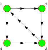
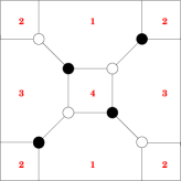
$a=\left(\begin{array}[]{cccc}0&2&-4&2\\ -2&0&2&0\\ 4&-2&0&-2\\ -2&0&2&0\end{array}\right)$

Figure 7: Quiver, brane tiling, toric diagram and adjacency matrix for $\mathbb{F}_{0}^{(II)}$

The external and internal perfect matchings are represented in Figure 8 and 9 respectively. They respect the relations

$$\pi_{1}+\pi_{2}=\sigma_{2}+\sigma_{5},\quad\pi_{1}+\pi_{2}-\pi_{3}-\pi_{4}=\sigma_{2}-\sigma_{4},\quad\pi_{1}+\pi_{2}-\pi_{3}-\pi_{4}=2\sigma_{2}-\sigma_{1}-\sigma_{3}$$

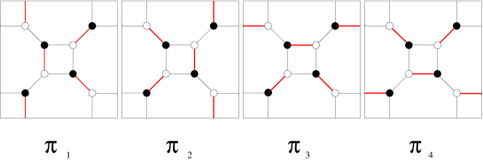
Figure 8: External perfect matchings of $\mathbb{F}_{0}^{(II)}$

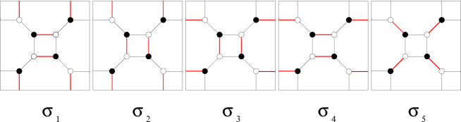
Figure 9: Internal perfect matchings of $\mathbb{F}_{0}^{(II)}$

while $T$ results

$$T=\left(\begin{array}[]{ccccccccc}\pi_{1}&\pi_{2}&\pi_{3}&\pi_{4}&\sigma_{1}&\sigma_{2}&\sigma_{3}&\sigma_{4}&\sigma_{5}\\ 0&1&0&0&0&0&-1&-1&1\\ 1&0&0&0&0&0&-1&-1&1\\ 0&0&1&0&0&0&1&1&0\\ 0&0&0&1&0&0&1&1&0\\ 0&0&0&0&1&0&-1&0&0\\ 0&0&0&0&0&1&2&1&-1\end{array}\right)$$ (55)

The loops are identified with the differences among these perfect matchings as

$$w_{1}=\frac{y_{\delta\sigma_{1}}}{y_{\delta\sigma_{5}}},\quad w_{2}=\frac{y_{\delta\sigma_{3}}}{y_{\delta\sigma_{2}}},\quad w_{3}=\frac{y_{\delta\sigma_{5}}}{y_{\delta\sigma_{3}}},\quad w_{4}=\frac{y_{\delta\sigma_{2}}}{y_{\delta\sigma_{1}}}$$ (56)

By fixing the first perfect matching as the reference one, we obtain the $\delta T$ matrix as

$$\delta T=\left(\begin{array}[]{ccccccccc}0&1&0&0&0&0&-1&-1&1\\ 0&-1&-1&-1&-1&-1&-2&-2&0\\ 0&0&1&0&0&0&1&1&0\\ 0&0&0&1&0&0&1&1&0\\ 0&0&0&0&1&0&-1&0&0\\ 0&0&0&0&0&1&2&1&-1\end{array}\right)$$ (57)

The matrix $B$ and $A$ as defined in (22) and (25) are

$$B=\left(\begin{array}[]{cccccc}-1&-1&-1&-1&-1&1\\ 1&0&0&-1&-1&1\\ 0&1&0&-1&-1&1\\ 0&0&1&-1&-1&1\\ 0&0&0&0&4&1\\ 0&0&0&4&0&1\end{array}\right)\quad A=\left(\begin{array}[]{cccc}-1&-1&2&0\\ -1&-1&2&0\\ 0&1&-1&0\\ 0&1&-1&0\\ 1&-1&1&-1\\ 1&1&-3&1\end{array}\right)$$ (58)

Once again the CY condition of the master space guarantees that we can express all the closed cycles on the dimer as combination of the first $5$ columns of the matrix $B$, whereas the last column is the orthogonal direction. We associate to the first $5$ columns the following local coordinates $x_{m}$ on the Poisson manifold

$$\{x_{m}\}=(c_{1},c_{2},c_{3},q_{1},q_{2})$$ (59)

where the $c_{e}$ are associated to Casimir, while $q_{1}$ and $q_{2}$ are dynamical variables. By solving (27) the antisymmetric structure among these charges is

$$\{c_{e},c_{f}\}=0,\quad\{c_{e},q_{\widetilde{n}}\}=\{q_{\widetilde{m}},c_{f}\}=0,\quad\{q_{\widetilde{m}},q_{\widetilde{n}}\}=-16\,\epsilon_{\widetilde{m}\widetilde{n}}$$ (60)

The $y$ variables in terms of the $c_{i}$ and $q_{i}$ become

$$y_{\delta\sigma_{1}}=e^{\frac{c_{1}}{4}+\frac{c_{2}}{4}+\frac{c_{3}}{4}+\frac{q_{2}}{4}}\quad\,\,\,,\,\,\,y_{\delta\sigma_{2}}=e^{\frac{c_{1}}{4}+\frac{c_{2}}{4}+\frac{c_{3}}{4}+\frac{q_{1}}{4}},\quad y_{\delta\sigma_{3}}=e^{-\frac{3c_{1}}{4}+\frac{5c_{2}}{4}+\frac{5c_{3}}{4}+\frac{q_{1}}{2}-\frac{q_{2}}{4}}$$

$$y_{\delta\sigma_{4}}=e^{-\frac{3c_{1}}{4}+\frac{5c_{2}}{4}+\frac{5c_{3}}{4}+\frac{q_{1}}{4}},\,\,\,y_{\delta\sigma_{5}}=e^{\frac{3c_{1}}{4}-\frac{c_{2}}{4}-\frac{c_{3}}{4}-\frac{q_{1}}{4}}$$ (61)

The only Hamiltonian corresponding to the single internal point is

$$H=y_{\delta\sigma_{1}}+y_{\delta\sigma_{2}}+y_{\delta\sigma_{3}}+y_{\delta\sigma_{4}}+y_{\delta\sigma_{5}}$$ (62)

Finally, by introducing the paths $z_{1}$ and $z_{2}$ as

$$z_{1}=\frac{y_{\delta\sigma_{5}}}{y_{\delta\pi_{1}}},\quad z_{2}=\frac{y_{\delta\sigma_{9}}}{y_{\delta\pi_{3}}}$$ (63)

we reconstruct the algebra of the $w_{i}$ and $z_{1}$ and $z_{2}$ from (60). we have

$$\left(\begin{array}[]{c|c}\frac{\{w_{A},w_{B}\}}{w_{A}w_{B}}&\frac{\{w_{A},z_{t}\}}{w_{A}z_{t}}\\ \hline\cr\frac{\{z_{u},w_{B}\}}{z_{u}w_{B}}&\frac{\{z_{u},z_{t}\}}{z_{u}z_{t}}\end{array}\right)=\left(\begin{array}[]{cccccc}0&2&-4&2&-1&-1\\ -2&0&2&0&1&1\\ 4&-2&0&-2&-1&-1\\ -2&0&2&0&1&1\\ 1&-1&1&-1&0&0\\ 1&-1&1&-1&0&0\end{array}\right)$$ (64)

5.2 Theories with multiple Hamiltonians

In the sections above we studied models with a single internal point, i.e. one Hamiltonian. The local coordinate system we have provided reproduces the correct intersection pairing and allows to extract the canonical variables. These systems are trivially integrable, since there is one Hamiltonian for a phase space of dimension two. In this section we apply our algorithm to models with multiple internal points $I$. In such models the integrability is non trivial and is guaranteed by the existence of $I$ Hamiltonians in involution Goncharov:2011hp .

We study in detail some $Y^{p0}$ example, which have been shown in Eager:2011dp to have the same spectral curve of the Toda chain, in the non relativistic limit. We introduce the local coordinate system associated to the $U(1)$ charges, we extract the corresponding Poisson structure, and we show that the $I$ Hamiltonians are indeed in involutions. This provide a further consistency check of our algorithm and of the local coordinatization of the Poisson manifold, based on the master space. We restrict the examples to the case of the $Y^{p0}$ quiver gauge theories, but our algorithm can be applied to all the infinite classes $Y^{pq}$Benvenuti:2004dy and $L^{pqr}$ Benvenuti:2005ja ; Butti:2005sw ; Franco:2005sm of toric $\mathcal{N}=1$ SCFT. With this procedure one can construct explicitly the corresponding infinite classes of integrable systems and express the Hamiltonians in terms of local coordinates, and ultimately of canonical variables.

In the following examples we will not give all the details of the computation of the the master space. We leave to the appendix C these straightforward derivations.

5.2.1 $Y^{30}$

Here we study the $\mathcal{N}=1$ SCFT living on D$3$ branes probing the toric $Y^{30}$ singularity Benvenuti:2004dy . The quiver gauge theory, the tiling, the toric diagram and the adjacency matrix are depicted in Figure 10 and the superpotential is

$$W = X_{61}^{(1)}X_{12}X_{23}^{(2)}X_{36}-X_{61}^{(2)}X_{12}X_{23}^{(1)}X_{36}+X_{61}^{(2)}X_{14}X_{45}^{(1)}X_{56}$$ (65)

$$-X_{61}^{(1)}X_{14}X_{45}^{(2)}X_{56}+X_{23}^{(1)}X_{34}X_{45}^{(2)}X_{52}-X_{23}^{(2)}X_{34}X_{45}^{(1)}X_{52}$$

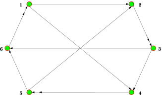
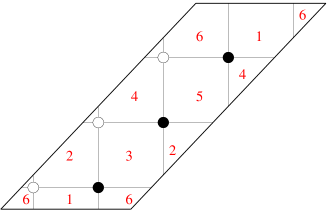
$a=\left(\begin{array}[]{cccccc}0&1&0&1&0&-2\\ -1&0&2&0&-1&0\\ 0&-2&0&1&0&1\\ -1&0&-1&0&2&0\\ 0&1&0&-2&0&1\\ 2&0&-1&0&-1&0\end{array}\right)$

Figure 10: Quiver, brane tiling, toric diagram and adjacency matrix for $Y^{(30)}$

In the appendix C we show both the external and the internal perfect matchings. They are relate by the relations

$$\pi_{2}+\pi_{4}=\sigma_{1}^{1}+\sigma_{4}^{1},\quad\pi_{4}=\sigma_{2}^{1}-\sigma_{3}^{1}+\sigma_{2}^{2},\quad\pi_{2}+\pi_{4}=\sigma_{2}^{1}+\sigma_{6}^{1},\quad\pi_{4}=\sigma_{2}^{1}+\sigma_{4}^{1}-\sigma_{5}^{2}$$

$$\pi_{1}+\pi_{2}+\pi_{3}+2\pi_{4}=\sigma_{2}^{1}+\sigma_{4}^{1}+\sigma_{5}^{1}+\sigma_{1}^{2}+\sigma_{2}^{2},\quad\pi_{4}=\sigma_{4}^{1}+\sigma_{1}^{2}-\sigma_{6}^{2}$$

$$\pi_{1}+\pi_{3}+\pi_{4}=\sigma_{1}^{2}+\sigma_{2}^{2}+\sigma_{3}^{2},\quad\pi_{2}+2\pi_{4}=\sigma_{2}^{1}+\sigma_{4}^{1}+\sigma_{4}^{2}$$

The $T$ matrix encoding all the charges information of the $16$ perfect matchings which generate the master space results

$$T=\left(\begin{array}[]{cccccccccccccccc}\pi_{1}&\pi_{2}&\pi_{3}&\pi_{4}&\sigma^{2}_{2}&\sigma^{2}_{1}&\sigma^{1}_{4}&\sigma^{1}_{2}&\sigma^{2}_{4}&\sigma^{2}_{3}&\sigma^{2}_{6}&\sigma^{1}_{5}&\sigma^{2}_{5}&\sigma^{1}_{6}&\sigma^{1}_{3}&\sigma^{1}_{1}\\ 1&0&0&0&0&0&0&0&1&-1&1&0&0&1&-1&1\\ 0&1&0&0&0&0&0&0&1&0&1&0&1&1&0&0\\ 0&0&1&0&0&0&0&0&1&-1&1&0&0&1&-1&1\\ 0&0&0&1&0&0&0&0&1&0&0&1&0&1&0&1\\ 0&0&0&0&1&0&0&0&0&1&-1&1&-1&-1&0&0\\ 0&0&0&0&0&1&0&0&-1&1&-1&0&0&-1&1&0\\ 0&0&0&0&0&0&1&0&-1&1&0&0&0&-1&1&-1\\ 0&0&0&0&0&0&0&1&-1&0&0&-1&1&0&1&-1\end{array}\right)$$ (66)

The loops surrounding the faces of the dimer are associated to the differences

$$w_{1}=\frac{y_{\delta\sigma_{4}^{2}}}{y_{\delta\sigma_{6}^{2}}}\quad w_{2}=\frac{y_{\delta\sigma_{2}^{2}}}{y_{\delta\sigma_{4}^{2}}}\quad w_{3}=\frac{y_{\delta\sigma_{3}^{1}}}{y_{\delta\sigma_{2}^{1}}}\quad w_{4}=\frac{y_{\delta\sigma_{1}^{2}}}{y_{\delta\sigma_{3}^{2}}}\quad w_{5}=\frac{y_{\delta\sigma_{6}^{1}}}{y_{\delta\sigma_{1}^{1}}}\quad w_{6}=\frac{y_{\delta\sigma_{4}^{1}}}{y_{\delta\sigma_{3}^{1}}}$$ (67)

We consider as the reference perfect matching the first column of the matrix $T$, we then construct the matrix $\delta T$, and hence the base $B$. The matrices $B$ and $A$ then results

$$B=\left(\begin{array}[]{cccccccc}1&0&0&-1&-1&-1&-1&1\\ 0&1&0&-1&-1&-1&-1&1\\ 0&0&1&-1&-1&-1&-1&1\\ -1&-1&-1&-1&-1&-1&-1&1\\ 0&0&0&0&0&0&4&1\\ 0&0&0&0&0&4&0&1\\ 0&0&0&0&4&0&0&1\\ 0&0&0&4&0&0&0&1\end{array}\right)\quad\quad A=\left(\begin{array}[]{cccccc}0&-1&-1&1&0&1\\ 0&-1&0&0&1&0\\ 0&-1&-1&1&0&1\\ 1&-1&0&0&0&0\\ 1&1&0&-1&-1&0\\ 0&1&1&0&-1&-1\\ -1&1&1&-1&0&0\\ -1&1&0&0&1&-1\end{array}\right)$$ (68)

As usual the last column of the matrix $B$ represents the orthogonal direction that we discard. The first $g+1=7$ columns correspond to local coordinates on the Poisson manifold, which we label as $\{x_{m}\}=(c_{e},q_{\widetilde{m}})$, with $e=1,\dots,d-1$ and $\widetilde{m}=1,\dots,2I$. Here $d=4$ and $I=2$.

The first $3$ variables $c_{e}$ are associated to Casimir operators and they commute with everything. The other four $q_{\widetilde{m}}$ variables are dynamical and their Poisson bracket is found by solving (27). We have

$$\{q_{\widetilde{m}},q_{\widetilde{n}}\}=16\left(\begin{array}[]{cccc}0&\,\,1&0&0\\ -1&0&0&0\\ 0&0&0&-1\\ 0&0&\,\,1&0\end{array}\right)\qquad\widetilde{m},\widetilde{n}=1,\dots,4$$ (69)

The $y$ variables associated to the external points are

$$y_{\delta\pi_{1}}=1\quad y_{\delta\pi_{2}}=e^{c_{1}}\quad y_{\delta\pi_{3}}=e^{c_{2}}\quad y_{\delta\pi_{4}}=e^{c_{3}}$$ (70)

The $y$ variables associated to the first internal point are

$$\begin{array}[]{lll}y_{\delta\sigma_{1}^{1}}=e^{c_{1}+\frac{q_{1}}{4}-\frac{q_{4}}{4}},&y_{\delta\sigma_{2}^{1}}=e^{\frac{1}{4}\left(c_{1}+c_{2}+c_{3}-q_{2}-q_{3}-q_{4}\right)},&y_{\delta\sigma_{3}^{1}}=e^{\frac{1}{4}\left(2c_{1}+2c_{2}-2c_{3}-q_{3}-q_{4}\right)}\\ y_{\delta\sigma_{4}^{1}}=e^{\frac{1}{4}\left(c_{1}+c_{2}+c_{3}-q_{2}-q_{3}-q_{4}\right)},&y_{\delta\sigma_{5}^{1}}=e^{\frac{1}{4}\left(c_{1}+c_{2}+c_{3}+q_{3}\right)},&y_{\delta\sigma_{6}^{1}}=e^{\frac{1}{4}\left(3c_{1}-c_{2}+3c_{3}+q_{2}+q_{3}+q_{4}\right)}\end{array}$$ (71)

The $y$ variables associated to the second internal point are

$$\begin{array}[]{lll}y_{\delta\sigma_{1}^{2}}=e^{\frac{1}{4}\left(c_{1}+c_{2}+c_{3}+q_{1}\right)},&y_{\delta\sigma_{2}^{2}}=e^{\frac{1}{4}\left(c_{1}+c_{2}+c_{3}+q_{2}\right)},&y_{\delta\sigma_{3}^{2}}=e^{\frac{1}{4}\left(-2c_{1}+2c_{2}+2c_{3}-q_{1}-q_{2}\right)}\\ y_{\delta\sigma_{4}^{2}}=e^{\frac{1}{4}\left(3c_{1}-c_{2}+3c_{3}+q_{1}+q_{2}+q_{3}\right)},&y_{\delta\sigma_{5}^{2}}=e^{\frac{1}{4}\left(c_{1}+c_{2}+c_{3}-q_{1}-q_{2}-q_{3}\right)},&y_{\delta\sigma_{6}^{2}}=e^{\frac{1}{4}\left(c_{1}+c_{2}+c_{3}+q_{4}\right)}\end{array}$$ (72)

The Hamiltonians are

$$H^{a}=\sum_{k_{a}=1}^{6}y_{\delta\sigma_{k_{a}}^{a}}\quad\quad a=1,2$$ (73)

and they commute given the algebra (69). The expressions (69) and (73) determine explicitly the integrable system associated to the $Y^{30}$ quiver gauge theory. The local coordinates can be made canonical by transforming the antisymmetric structure to a canonical block diagonal form. Finally, by defining the $z_{u}$ as

$$z_{1}=\frac{y_{\delta\sigma_{5}^{2}}}{y_{\delta\sigma_{6}^{1}}},\quad z_{2}=\frac{y_{\delta\pi_{1}}}{y_{\delta\pi_{4}}}$$ (74)

we obtain the intersection matrix for the base of cycles $w_{A},z_{1},z_{2}$, by considering them as exponential functions of the local coordinates $x_{m}=(c_{1},c_{2},c_{3},q_{1},q_{2},q_{3},q_{4})$ and by using the antisymmetric structure (69). We have

$$\left(\begin{array}[]{c|c}\frac{\{w_{A},w_{B}\}}{w_{A}w_{B}}&\frac{\{w_{A},z_{t}\}}{w_{A}z_{t}}\\ \hline\cr\frac{\{z_{u},w_{B}\}}{z_{u}w_{B}}&\frac{\{z_{u},z_{t}\}}{z_{u}z_{t}}\end{array}\right)=\left(\begin{array}[]{cccccccc}0&1&0&1&0&-2&1&0\\ -1&0&2&0&-1&0&1&0\\ 0&-2&0&1&0&1&-1&0\\ -1&0&-1&0&2&0&0&0\\ 0&1&0&-2&0&1&0&0\\ 2&0&-1&0&-1&0&-1&0\\ -1&-1&1&0&0&1&0&0\\ 0&0&0&0&0&0&0&0\end{array}\right)$$ (75)

One can check that this matrix is the same that can be obtained from the intersection index for cycles (10) of Goncharov:2011hp that we review in the appendix A. This further confirms the validity of our construction of local coordinates on the Poisson manifold and their associated Poisson structure.

5.2.2 $Y^{40}$

The last example with multiple internal points is the $\mathcal{N}=1$ SCFT living on D$3$ branes probing the toric $Y^{40}$ singularity Benvenuti:2004dy . The quiver gauge theory, the tiling, the toric diagram and the adjacency matrix are depicted in Figure 11 and the superpotential is

$$W = X_{15}^{(1)}X_{58}X_{84}^{(2)}X_{41}-X_{15}^{(2)}X_{58}X_{84}^{(1)}X_{41}+X_{15}^{(2)}X_{56}X_{62}^{(1)}X_{21}-X_{15}^{(1)}X_{56}X_{62}^{(2)}X_{21}$$

$$+ X_{62}^{(2)}X_{23}X_{37}^{(1)}X_{76}-X_{62}^{(1)}X_{23}X_{37}^{(2)}X_{76}+X_{37}^{(2)}X_{78}X_{84}^{(1)}X_{43}-X_{37}^{(1)}X_{78}X_{84}^{(2)}X_{43}$$

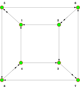
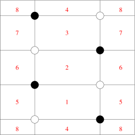
$a=\left(\begin{array}[]{cccccccc}0&-1&0&-1&2&0&0&0\\ 1&0&1&0&0&-2&0&0\\ 0&-1&0&-1&0&0&2&0\\ 1&0&1&0&0&0&0&-2\\ -2&0&0&0&0&1&0&1\\ 0&2&0&0&-1&0&-1&0\\ 0&0&-2&0&0&1&0&1\\ 0&0&0&2&-1&0&-1&0\end{array}\right)$

Figure 11: Quiver, brane tiling, toric diagram and adjacency matrix for $Y^{(40)}$

In the appendix C we have shown the both the external and the internal perfect matchings. The perfect matchings satisfy the following relations

$$\pi_{2}+\pi_{3}=-\sigma_{1}^{2}+\sigma_{2}^{2}-\sigma_{2}^{3}+\sigma_{5}^{2}+\sigma_{7}^{2}+\sigma_{8}^{3},\,\,\pi_{3}=\sigma_{2}^{3}-\sigma_{5}^{2}+\sigma_{6}^{3},\,\,\pi_{3}=-\sigma_{2}^{2}+\sigma_{2}^{3}+\sigma_{5}^{3}$$

$$\pi_{2}+\pi_{3}=-\sigma_{1}^{2}+\sigma_{5}^{2}+\sigma_{7}^{2}+\sigma_{16}^{2},\,\,\pi_{1}+\pi_{3}+\pi_{4}=\sigma_{1}^{2}+\sigma_{1}^{3}+\sigma_{7}^{3}$$

$$\pi_{2}+\pi_{3}=\sigma_{1}^{2}+\sigma_{2}^{2}+\sigma_{7}^{2}+\sigma_{15}^{2},\,\,\pi_{2}+\pi_{3}=\sigma_{1}^{2}+\sigma_{2}^{3}+\sigma_{7}^{2}+\sigma_{8}^{1},\,\,\pi_{3}=-\sigma_{2}^{2}+2\sigma_{2}^{3}-\sigma_{5}^{2}+\sigma_{14}^{2}$$

$$\pi_{1}+\pi_{3}+\pi_{4}=\sigma_{1}^{2}+\sigma_{1}^{3}+\sigma_{2}^{3}-\sigma_{5}^{2}+\sigma_{13}^{2}\quad\pi_{2}+\pi_{3}=-2\sigma_{1}^{2}+\sigma_{2}^{2}+\sigma_{5}^{2}+\sigma_{7}^{2}+\sigma_{12}^{2}$$

$$\pi_{3}=-\sigma_{1}^{2}+\sigma_{2}^{3}+\sigma_{4}^{3},\,\,\pi_{2}=\sigma_{2}^{2}-2\sigma_{2}^{3}+\sigma_{5}^{2}+\sigma_{11}^{2},\,\,\sigma_{1}^{2}-\sigma_{2}^{3}+\sigma_{3}^{3}-\sigma_{7}^{2}=0$$

$$\sigma_{1}^{2}-\sigma_{2}^{2}-\sigma_{7}^{2}+\sigma_{10}^{2}=0\quad\sigma_{1}^{2}-\sigma_{5}^{2}-\sigma_{7}^{2}+\sigma_{8}^{2}=0,\,\,\pi_{1}+\pi_{4}=2\sigma_{1}^{2}+\sigma_{1}^{3}-\sigma_{2}^{3}-\sigma_{7}^{2}+\sigma_{9}^{2}$$

$$\pi_{2}=\sigma_{2}^{2}-\sigma_{2}^{3}+\sigma_{6}^{1},\,\,\pi_{2}=-\sigma_{2}^{3}+\sigma_{5}^{2}+\sigma_{7}^{1}\quad\sigma_{1}^{2}-\sigma_{2}^{2}+\sigma_{2}^{3}-\sigma_{5}^{2}+\sigma_{5}^{1}-\sigma_{7}^{2}=0$$

$$\pi_{1}+\pi_{4}=2\sigma_{1}^{2}+\sigma_{1}^{3}+\sigma_{4}^{1}-\sigma_{5}^{2}-\sigma_{7}^{2},\,\,\pi_{2}=2-\sigma_{1}^{2}+\sigma_{2}^{2}-\sigma_{2}^{3}+\sigma_{3}^{1}+\sigma_{5}^{2},\,\,\sigma_{2}^{2}-\sigma_{2}^{3}-\sigma_{2}^{1}+\sigma_{5}^{2}=0$$

$$\pi_{2}=-\sigma_{1}^{2}-\sigma_{1}^{3}+\sigma_{2}^{2}-\sigma_{2}^{3}+\sigma_{4}^{2}+\sigma_{5}^{2}+\sigma_{7}^{2},\,\,\pi_{2}=-\sigma_{1}^{2}-\sigma_{1}^{3}+\sigma_{1}^{1}+\sigma_{5}^{2}+\sigma_{7}^{2}$$

$$\sigma_{1}^{3}+\sigma_{2}^{2}-\sigma_{2}^{3}-\sigma_{3}^{2}=0,\,\,\pi_{1}+\pi_{4}=2\sigma_{1}^{2}$$ (77)

The $T$ matrix encoding all the charges information of the $36$ perfect matchings which generate the master space results

$$T\!=\!\left(\!\!\begin{array}[]{cccccccccccccccccccccccccccccccccccc}\pi_{1}&\pi_{2}&\pi_{3}&\pi_{4}&\sigma^{2}_{2}&\sigma^{2}_{6}&\sigma^{3}_{1}&\sigma^{2}_{7}&\sigma^{2}_{5}&\sigma^{3}_{2}&\sigma^{2}_{1}&\sigma^{2}_{3}&\sigma^{1}_{1}&\sigma^{2}_{4}&\sigma^{1}_{2}&\sigma^{1}_{3}&\sigma^{1}_{4}&\sigma^{1}_{5}&\sigma^{1}_{7}&\sigma^{2}_{8}&\sigma^{1}_{6}&\sigma^{2}_{9}&\sigma^{2}_{10}&\sigma^{3}_{3}&\sigma^{2}_{11}&\sigma^{3}_{4}&\sigma^{2}_{12}&\sigma^{2}_{13}&\sigma^{2}_{14}&\sigma^{1}_{8}&\sigma^{2}_{15}&\sigma^{3}_{7}&\sigma^{5}_{7}&\sigma^{2}_{16}&\sigma^{6}_{5}&\sigma^{3}_{8}\\ 1&0&0&0&0&0&0&0&0&0&1&0&0&0&0&0&1&0&0&0&0&1&0&0&0&0&0&1&0&0&0&1&0&0&0&0\\ 0&1&0&0&0&0&0&0&0&0&0&0&1&1&0&1&0&0&1&0&1&0&0&0&1&0&1&0&0&1&1&0&0&1&0&1\\ 0&0&1&0&0&0&0&0&0&0&0&0&0&0&0&0&0&0&0&0&0&0&0&0&0&1&1&1&1&1&1&1&1&1&1&1\\ 0&0&0&1&0&0&0&0&0&0&1&0&0&0&0&0&1&0&0&0&0&1&0&0&0&0&0&1&0&0&0&1&0&0&0&0\\ 0&0&0&0&1&0&0&0&0&0&\!-1&0&1&1&0&1&\!-2&\!-1&0&\!-1&0&\!-2&\!-1&\!-1&0&1&2&\!-1&0&1&1&\!-1&0&1&0&1\\ 0&0&0&0&0&1&0&0&0&0&0&1&0&\!-1&1&\!-1&0&1&0&0&\!-1&0&1&0&\!-1&0&\!-1&0&1&0&\!-1&0&1&0&0&\!-1\\ 0&0&0&0&0&0&1&0&0&0&0&1&1&1&0&0&\!-1&0&0&0&0&\!-1&0&0&0&0&0&\!-1&0&0&0&\!-1&0&0&0&0\\ 0&0&0&0&0&0&0&1&0&0&0&0&\!-1&\!-1&0&0&1&1&0&1&0&1&1&1&0&0&\!-1&0&0&\!-1&\!-1&0&0&\!-1&0&\!-1\\ 0&0&0&0&0&0&0&0&1&0&0&0&\!-1&\!-1&1&\!-1&1&1&\!-1&1&0&0&0&0&\!-1&0&\!-1&1&1&0&0&0&0&\!-1&1&\!-1\\ 0&0&0&0&0&0&0&0&0&1&0&\!\!-1\!&0&1&\!-1&1&0&\!-1&1&0&1&1&0&1&2&\!-1&0&\!-1&\!-2&\!-1&0&0&\!-1&0&\!-1&1\end{array}\!\right)$$ (78)

The loops around the faces of the tiling can be written in term of the $y$ variables as

$$w_{1}=\frac{y_{\delta\sigma_{4}^{2}}}{y_{\delta\sigma_{1}^{2}}},\,w_{2}=\frac{y_{\delta\sigma_{3}^{1}}}{y_{\delta\sigma_{6}^{1}}},\,w_{3}=\frac{y_{\delta\sigma_{14}^{2}}}{y_{\delta\sigma_{3}^{2}}},\,w_{4}=\frac{y_{\delta\sigma_{2}^{1}}}{y_{\delta\sigma_{8}^{1}}},\,w_{5}=\frac{y_{\delta\sigma_{4}^{1}}}{y_{\delta\sigma_{5}^{1}}},\,w_{6}=\frac{y_{\delta\sigma_{6}^{2}}}{y_{\delta\sigma_{2}^{2}}},\,w_{7}=\frac{y_{\delta\sigma_{2}^{3}}}{y_{\delta\sigma_{10}^{2}}},\,w_{8}=\frac{y_{\delta\sigma_{5}^{1}}}{y_{\delta\sigma_{2}^{1}}}$$

We consider as the reference perfect matching the first column of the matrix $T$, we then construct the matrix $\delta T$, and hence the base $B$. The matrices $B$ and $A$ then results

$$B=\left(\begin{array}[]{cccccccccc}-1&-1&-1&-1&-1&-1&-1&-1&-1&1\\ 1&0&0&-1&-1&-1&-1&-1&-1&1\\ 0&1&0&-1&-1&-1&-1&-1&-1&1\\ 0&0&1&-1&-1&-1&-1&-1&-1&1\\ 0&0&0&0&0&0&0&0&4&1\\ 0&0&0&0&0&0&0&4&0&1\\ 0&0&0&0&0&0&4&0&0&1\\ 0&0&0&0&0&4&0&0&0&1\\ 0&0&0&0&4&0&0&0&0&1\\ 0&0&0&4&0&0&0&0&0&1\end{array}\right)\quad\quad A=\left(\begin{array}[]{cccccccc}-1&0&0&0&1&0&0&0\\ 1&0&0&-1&0&0&0&0\\ 0&0&1&-1&0&0&0&0\\ -1&0&0&0&1&0&0&0\\ 2&1&0&-1&-1&-1&1&-1\\ -1&0&0&1&-1&1&0&0\\ 1&0&-1&0&-1&0&1&0\\ -1&0&0&1&0&0&-1&1\\ -1&-1&1&1&0&0&0&0\\ 1&0&-1&0&1&0&-1&0\end{array}\right)$$ (79)

As usual we can define the $c$ and $q$ variables, and we have $\{x_{m}\}=(c_{e},q_{\widetilde{m}})$, with $e=1,\dots,d-1$ and $\widetilde{m}=1,\dots,2I$. Here $d=4$ and $I=3$. The $c_{e}$ commute with everything and they are related to the Casimir operators while the $q_{\widetilde{m}}$ algebra becomes

$$\{q_{\widetilde{m}},q_{\widetilde{n}}\}=16\left(\begin{array}[]{cccccc}\,0&\,0&-1&-1&\,0&\,0\\ \,0&\,0&-2&\,0&\,0&-1\\ \,1&\,2&\,0&\,0&\,0&\,1\\ \,1&\,0&\,0&\,0&1&\,0\\ \,0&\,0&\,0&-1&\,0&\,1\\ \,0&\,1&-1&\,0&-1&\,0\end{array}\right)\quad\quad\widetilde{m},\widetilde{n}=1,\dots,6$$ (80)

The $y$ variables can be expressed in terms of the $c_{e}$ and $q_{\widetilde{m}}$ by looking at the matrix $B^{-1}\delta T$. The $y$ associated to the external perfect matchings are

$$y_{\delta\pi_{1}}=1\quad y_{\delta\pi_{2}}=e^{c_{1}}\quad y_{\delta\pi_{3}}=e^{c_{2}}\quad y_{\delta\pi_{4}}=e^{c_{3}}$$ (81)

The $y$ associated to the internal perfect matchings are the exponential of the sub-sector of $B^{-1}\delta T$ describing the internal perfect matchings. This is

$$\left(\!\!\begin{array}[]{c|cccccccccccccccccccccccccccccccc}&\delta\sigma^{2}_{2}\!&\!\delta\sigma^{2}_{6}\!&\!\delta\sigma^{3}_{1}\!&\!\delta\sigma^{2}_{7}\!&\!\delta\sigma^{2}_{5}\!&\!\delta\sigma^{3}_{2}\!&\!\delta\sigma^{2}_{1}\!&\!\delta\sigma^{2}_{3}\!&\!\delta\sigma^{1}_{1}\!&\!\delta\sigma^{2}_{4}\!&\!\delta\sigma^{1}_{2}\!&\!\delta\sigma^{1}_{3}\!&\!\delta\sigma^{1}_{4}\!&\!\delta\sigma^{1}_{5}\!&\!\delta\sigma^{1}_{7}\!&\!\delta\sigma^{2}_{8}\!&\!\delta\sigma^{1}_{6}\!&\!\delta\sigma^{2}_{9}\!&\!\delta\sigma^{2}_{10}\!&\!\delta\sigma^{3}_{3}\!&\!\delta\sigma^{2}_{11}\!&\!\delta\sigma^{3}_{4}\!&\!\delta\sigma^{2}_{12}\!&\!\delta\sigma^{2}_{13}\!&\!\delta\sigma^{2}_{14}\!&\!\delta\sigma^{1}_{8}\!&\!\delta\sigma^{2}_{15}\!&\!\delta\sigma^{3}_{7}\!&\!\delta\sigma^{5}_{7}\!&\!\delta\sigma^{2}_{16}\!&\!\delta\sigma^{6}_{5}\!&\!\delta\sigma^{3}_{8}\\ \hline\cr c_{1}&\frac{1}{4}&\frac{1}{4}&\frac{1}{4}&\frac{1}{4}&\frac{1}{4}&\frac{1}{4}&\!\!-\frac{1}{4}&\frac{1}{4}&1&1&\frac{1}{4}&1&\!\!-\frac{1}{4}&\frac{1}{4}&1&\frac{1}{4}&1&\!\!-\frac{1}{4}&\frac{1}{4}&\frac{1}{4}&1&0&\frac{3}{4}&\!\!-\frac{1}{2}&0&\frac{3}{4}&\frac{3}{4}&\!\!-\frac{1}{2}&0&\frac{3}{4}&0&\frac{3}{4}\\ c_{2}&\frac{1}{4}&\frac{1}{4}&\frac{1}{4}&\frac{1}{4}&\frac{1}{4}&\frac{1}{4}&\!\!-\frac{1}{4}&\frac{1}{4}&0&0&\frac{1}{4}&0&\!\!-\frac{1}{4}&\frac{1}{4}&0&\frac{1}{4}&0&\!\!-\frac{1}{4}&\frac{1}{4}&\frac{1}{4}&0&1&\frac{3}{4}&\frac{1}{2}&1&\frac{3}{4}&\frac{3}{4}&\frac{1}{2}&1&\frac{3}{4}&1&\frac{3}{4}\\ c_{3}&\frac{1}{4}&\frac{1}{4}&\frac{1}{4}&\frac{1}{4}&\frac{1}{4}&\frac{1}{4}&\frac{3}{4}&\frac{1}{4}&0&0&\frac{1}{4}&0&\frac{3}{4}&\frac{1}{4}&0&\frac{1}{4}&0&\frac{3}{4}&\frac{1}{4}&\frac{1}{4}&0&0&\!\!-\frac{1}{4}&\frac{1}{2}&0&\!\!-\frac{1}{4}&\!\!-\frac{1}{4}&\frac{1}{2}&0&\!\!-\frac{1}{4}&0&\!\!-\frac{1}{4}\\ q_{1}&0&0&0&0&0&\frac{1}{4}&0&\!\!-\frac{1}{4}&0&\frac{1}{4}&\!\!-\frac{1}{4}&\frac{1}{4}&0&\!\!-\frac{1}{4}&\frac{1}{4}&0&\frac{1}{4}&\frac{1}{4}&0&\frac{1}{4}&\frac{1}{2}&\!\!-\frac{1}{4}&0&\!\!-\frac{1}{4}&\!\!-\frac{1}{2}&\!\!-\frac{1}{4}&0&0&\!\!-\frac{1}{4}&0&\!\!-\frac{1}{4}&\frac{1}{4}\\ q_{2}&0&0&0&0&\frac{1}{4}&0&0&0&\!\!-\frac{1}{4}&\!\!-\frac{1}{4}&\frac{1}{4}&\!\!-\frac{1}{4}&\frac{1}{4}&\frac{1}{4}&\!\!-\frac{1}{4}&\frac{1}{4}&0&0&0&0&\!\!-\frac{1}{4}&0&\!\!-\frac{1}{4}&\frac{1}{4}&\frac{1}{4}&0&0&0&0&\!\!-\frac{1}{4}&\frac{1}{4}&\!\!-\frac{1}{4}\\ q_{3}&0&0&0&\frac{1}{4}&0&0&0&0&\!\!-\frac{1}{4}&\!\!-\frac{1}{4}&0&0&\frac{1}{4}&\frac{1}{4}&0&\frac{1}{4}&0&\frac{1}{4}&\frac{1}{4}&\frac{1}{4}&0&0&\!\!-\frac{1}{4}&0&0&\!\!-\frac{1}{4}&\!\!-\frac{1}{4}&0&0&\!\!-\frac{1}{4}&0&\!\!-\frac{1}{4}\\ q_{4}&0&0&\frac{1}{4}&0&0&0&0&\frac{1}{4}&\frac{1}{4}&\frac{1}{4}&0&0&\!\!-\frac{1}{4}&0&0&0&0&\!\!-\frac{1}{4}&0&0&0&0&0&\!\!-\frac{1}{4}&0&0&0&\!\!-\frac{1}{4}&0&0&0&0\\ q_{5}&0&\frac{1}{4}&0&0&0&0&0&\frac{1}{4}&0&\!\!-\frac{1}{4}&\frac{1}{4}&\!\!-\frac{1}{4}&0&\frac{1}{4}&0&0&\!\!-\frac{1}{4}&0&\frac{1}{4}&0&\!\!-\frac{1}{4}&0&\!\!-\frac{1}{4}&0&\frac{1}{4}&0&\!\!-\frac{1}{4}&0&\frac{1}{4}&0&0&\!\!-\frac{1}{4}\\ q_{6}&\frac{1}{4}&0&0&0&0&0&\!\!-\frac{1}{4}&0&\frac{1}{4}&\frac{1}{4}&0&\frac{1}{4}&\!\!-\frac{1}{2}&\!\!-\frac{1}{4}&0&\!\!-\frac{1}{4}&0&\!\!-\frac{1}{2}&\!\!-\frac{1}{4}&\!\!-\frac{1}{4}&0&\frac{1}{4}&\frac{1}{2}&\!\!-\frac{1}{4}&0&\frac{1}{4}&\frac{1}{4}&\!\!-\frac{1}{4}&0&\frac{1}{4}&0&\frac{1}{4}\end{array}\right)$$ (82)

The three Hamiltonians are

$$H^{1}=\sum_{k_{1}=1}^{8}y_{\delta\sigma_{k_{1}}^{1}}\quad,\quad H^{2}=\sum_{k_{2}=1}^{16}y_{\delta\sigma_{k_{2}}^{2}}\quad,\quad H^{3}=\sum_{k_{3}=1}^{8}y_{\delta\sigma_{k_{3}}^{3}}$$ (83)

and given the algebra (80) they commute one each other. Finally, by defining the $z$ as

$$z_{1}=\frac{y_{\delta\pi_{3}}}{y_{\delta\sigma_{5}^{3}}},\quad z_{2}=\frac{y_{\delta\pi_{4}}}{y_{\delta\sigma_{1}^{2}}}$$ (84)

we can obtain the intersection matrix for the base of cycles $w_{A},z_{1},z_{2}$. By considering them as exponential functions of the local coordinates $x_{m}=(c_{1},c_{2},c_{3},q_{1},q_{2},q_{3},q_{4},q_{5},q_{6})$ and by using the antisymmetric structure (80) we have

$$\left(\begin{array}[]{c|c}\frac{\{w_{A},w_{B}\}}{w_{A}w_{B}}&\frac{\{w_{A},z_{t}\}}{w_{A}z_{t}}\\ \hline\cr\frac{\{z_{u},w_{B}\}}{z_{u}w_{B}}&\frac{\{z_{t},z_{u}\}}{z_{t}z_{u}}\end{array}\right)=\left(\begin{array}[]{cccccccccc}0&-1&0&-1&2&0&0&0&0&0\\ 1&0&1&0&0&-2&0&0&0&0\\ 0&-1&0&-1&0&0&2&0&2&0\\ 1&0&1&0&0&0&0&-2&0&-2\\ -2&0&0&0&0&1&0&1&0&1\\ 0&2&0&0&-1&0&-1&0&-1&0\\ 0&0&-2&0&0&1&0&1&0&1\\ 0&0&0&2&-1&0&-1&0&-1&0\\ 0&0&-2&0&0&1&0&1&0&1\\ 0&0&0&2&-1&0&-1&0&-1&0\end{array}\right)$$ (85)

Even in this case this matrix coincide with the one obtained from the intersection index for cycles (10) of Goncharov:2011hp that we review in the appendix A.

6 Seiberg duality as a canonical transformation

In this section we discuss the interpretation of Seiberg duality as a canonical transformation that glues the different local patches of the cluster integrable model. The dimer integrable system depends on the multiplicity of the internal point of the toric diagram, in the structure of the Hamiltonians, and the Poisson structure is related to the anomalous global symmetries of the theory. Hence for chiral theories the dimer integrable systems is modified under Seiberg duality. However, by using the local parametrization introduced in the previous sections, one can verify that Seiberg duality acts on the coordinates as a canonical transformation

$$(c_{e},q_{\widetilde{m}})=(c_{e}(c_{f}^{S.d.}),q_{\widetilde{m}}(c_{f}^{S.d.},q_{\widetilde{n}}^{S.d.}))$$ (86)

Moreover, as we discussed in section 4 the toric data of the master spaces give canonical transformation that are linear maps among the Casimir operators and non linear maps for the $q$ variables. The first are realized by mapping the external perfect matching in the usual toric way and the second relations, among the internal perfect matchings, are obtained by equating the Hamiltonian functions and their flows.

Here we show the equivalence between this interpretation of the duality as a symplectic morphism on the master space and the description of Goncharov:2011hp in terms of mutation of the seed defining the cluster algebra.

6.1 Seiberg duality on $\mathbb{F}_{0}$

The transformation on the $c_{e}$ coordinates can be understood from the T matrix and equation (17). We have

$$c_{1}=c_{2}^{S.d.}\quad\quad c_{2}=c_{1}^{S.d.}\quad\quad c_{3}=c_{3}^{S.d.}$$ (87)

The transformation among the $q$ variables is obtained by solving the equations (18) and (19). The first equation is an algebraic equation and it reads

$$y_{\delta\sigma_{1}}+y_{\delta\sigma_{2}}+y_{\delta\sigma_{3}}+y_{\delta\sigma_{4}}=y_{\delta\sigma_{1}^{S.d.}}+y_{\delta\sigma_{2}^{S.d.}}+y_{\delta\sigma_{3}^{S.d.}}+y_{\delta\sigma_{4}^{S.d.}}+y_{\delta\sigma_{5}^{S.d.}}$$ (88)

The other two differential equations are

$$\!\!y_{\delta\sigma_{7}}\!-\!y_{\delta\sigma_{6}}=\left(y_{\delta\sigma_{6}^{S.d.}}+2y_{\delta\sigma_{7}^{S.d.}}+y_{\delta\sigma_{8}^{S.d.}}-y_{\delta\sigma_{9}^{S.d.}}\right)\partial_{q_{2}^{S.d.}}q_{2}+\left(y_{\delta\sigma_{7}^{S.d.}}-y_{\delta\sigma_{5}^{S.d.}}\right)\partial_{q_{1}^{S.d.}}q_{2}$$

$$\!\!y_{\delta\sigma_{5}}\!-\!y_{\delta\sigma_{8}}=\left(y_{\delta\sigma_{6}^{S.d.}}+2y_{\delta\sigma_{7}^{S.d.}}+y_{\delta\sigma_{8}^{S.d.}}-y_{\delta\sigma_{9}^{S.d.}}\right)\partial_{q_{2}^{S.d.}}q_{1}+\left(y_{\delta\sigma_{7}^{S.d.}}-y_{\delta\sigma_{5}^{S.d.}}\right)\partial_{q_{1}^{S.d.}}q_{1}$$

Once expressed in terms of the $q_{\widetilde{m}}$ variables these equations look complicate partial differential equations. We will show in the next section that the functions $q_{1}(c_{e}^{S.d.},q_{\widetilde{m}}^{S.d.})$ and $q_{2}(c_{e}^{S.d.},q_{\widetilde{m}}^{S.d.})$ which solve these equations coincide with the functions obtained by using the procedure of Goncharov:2011hp .

6.2 Duality as seed mutation

In this section we are describing the mapping among the dual phases as discussed in Goncharov:2011hp . For a more detailed derivation we refer the reader to the appendix B. The Seiberg duality on the dimer is referred to as a cluster Poisson transformation obtained by a mutation of the seed. This transformation is based on an operation on the bipartite graphs called spider move. This is a local operation on the bipartite graphs which acts as in Figure 12. The original dimer and the resulting dimer correspond to two different (Seiberg) phases of the same gauge theories. The adjacency matrix is different and the number of perfect matching is different. The dimension of the corresponding Poisson manifold is however the same ($g+1$), and also the number of Casimir operators ($d-1$). There is a precise mapping between the two phases that makes the integrable system equivalent. This is a map between functions on the Poisson manifolds. Functions which correspond to cycles which do not intersect the cycle $w_{X}$ do not change under the spider move and should be the same in the two phases. Functions corresponding to cycles which intersect non trivially with the cycle $w_{X}$ are modified as follows. We can decompose every cycle which intersects with $w_{X}$ in two pieces: one part which is external to the spider move and one part which is involved in the spider move. The former is not modified by the spider move and it is the same in the two phases. The latter part can be written as combination of the paths $\gamma,w_{X}$ in the Figure.

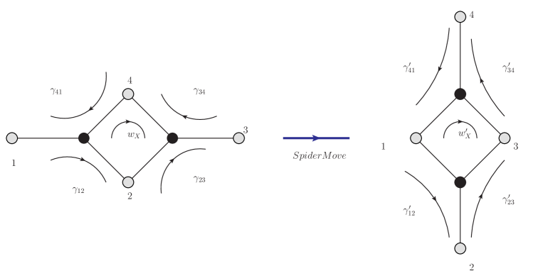
Figure 12: Spider move

In order for the two phases to describe two equivalent integrable systems, the paths in the two phases $\gamma,w_{X}$ and $\gamma^{\prime},w^{\prime}_{X}$ should be mapped as

$$\gamma_{41}\to\frac{\gamma_{41}^{\prime}}{(1+\frac{1}{w_{X}^{\prime}})},\,\gamma_{12}\to\gamma_{12}^{\prime}(1+w_{X}^{\prime}),\,\gamma_{23}\to\frac{\gamma_{23}^{\prime}}{(1+\frac{1}{w_{X}^{\prime}})},\,\gamma_{34}\to\gamma_{34}^{\prime}(1+w_{X}^{\prime}),\,w_{X}\to\frac{1}{w_{X}^{\prime}}$$ (90)

This mapping is translated in a map between functions in the two different phases. This mapping guarantees that the two integrable systems are equivalent.

6.2.1 The dual phases of $\mathbb{F}_{0}$

In this section we show the equivalence between the cluster Poisson transformation of Goncharov:2011hp and our derivation of Seiberg duality as a canonical transformation. The cluster Poisson transformation on the dimer is described by the spider move, combined with the integration of some massive field (if necessary). Indeed the two bipartite graphs describing the two phases of $\mathbb{F}_{0}$ cannot be immediately mapped by a spider move. However there is a simple operation in field theory which lead to recover the set up of spider move we have just explained. This operation consist of integrating in massive fields, which does not change the moduli space of the theory (and also the corresponding integrable system Goncharov:2011hp ). We integrate in some massive field on dimer of the first phase of $\mathbb{F}_{0}$ as in Figure 13.

Figure 13: Seiberg duality for $\mathbb{F}_{0}$: insertion of massive bifundamentals in $\mathbb{F}_{0}^{(I)}$ and spider move

In this description of $\mathbb{F}_{0}^{(I)}$ we can easily identify the face $w_{4}$ as face on which we can act with a spider move, i.e. that we can dualize. Indeed, by acting with a spider move on the fourth face one obtains the tiling of the dual phase, see Figure 13. This Figure shows that this combination of operation on the bipartite graphs gives the urban renewal 2001math…..11034P transformation, already observed to describe Seiberg duality on the bipartite graphs Franco:2005rj .

We are now interested in finding the transformation which map the cycles in the two dual phases. We consider the basis of cycles $w_{A},z_{1},z_{2}$ and $w^{\prime}_{A},z^{\prime}_{1},z^{\prime}_{2}$ as in section 5 for the two phases respectively. By following the discussion in Goncharov:2011hp that we just reviewed, the cycles can be factorized in two terms. One is related to the paths involved in the spider move and the second part is invariant under this transformation. In the phase $I$ this parametrization gives

$$w_{1}=w_{1}^{*}\gamma_{34}\gamma_{12},\quad w_{2}=w_{2}^{*},\quad\quad w_{3}=w_{3}^{*}\gamma_{41}\gamma_{23},\quad w_{4}=w_{X}\quad z_{1}=z_{1}^{*}\gamma_{23},\quad z_{2}=z_{2}^{*}\gamma_{34}^{-1}$$ (91)

whereas in phase $II$ gives

$$w_{1}^{\prime}=w_{1}^{*}\gamma^{\prime}_{34}\gamma^{\prime}_{12},\quad w_{2}^{\prime}=w_{2}^{*},\quad w_{3}^{\prime}=w_{3}^{*}\gamma^{\prime}_{41}\gamma^{\prime}_{23},\quad w_{4}^{\prime}=w^{\prime}_{X},\quad z_{1}^{\prime}=z_{1}^{*}\gamma^{\prime}_{23},\quad z_{2}^{\prime}=z_{2}^{*}\frac{1}{\gamma^{\prime}_{34}}$$ (92)

where we have denoted with $w^{*}$ the part of the cycle which is not modified by the spider move. The transformation we have explained in the previous section on the $\gamma,w_{X}$ then implies that the mapping among these cycles is

$$w_{1} = w_{1}^{\prime}(1+w_{4}^{\prime})^{2},\quad w_{2}=w_{2}^{\prime},\quad w_{3}=\frac{w_{3}^{\prime}}{(1+{w_{4}^{\prime}}^{-1})^{2}},\quad w_{4}={w_{4}^{\prime}}^{-1}$$

$$z_{1}~{} = \frac{z_{1}^{\prime}}{(1+{w_{4}^{\prime}}^{-1})},\quad z_{2}=\frac{z_{1}^{\prime}}{(1+{w_{4}^{\prime}}^{-1})}$$ (93)

In these expressions the mapping between cycles should be understood as a map between the corresponding functions, using the local coordinate systems that we introduced in the previous sections. For instance

$$w_{1}=e^{-\frac{c_{1}}{2}+\frac{c_{2}}{2}-\frac{c_{3}}{2}+\frac{q_{1}}{4}+\frac{q_{2}}{4}}=w_{1}^{\prime}(1+w_{4}^{\prime})^{2}=e^{-\frac{c_{1}^{S.d.}}{2}+\frac{c_{2}^{S.d.}}{2}+\frac{c_{3}^{S.d.}}{2}+\frac{q_{1}^{S.d.}}{4}+\frac{q_{2}^{S.d.}}{4}}\left(1+e^{\frac{q_{1}^{S.d.}}{4}-\frac{q_{2}^{S.d.}}{4}}\right)^{2}$$ (94)

and so on for the other $w_{A}$ and $z_{1},z_{2}$. A solution to these equations is given by

$$c_{1}=c_{2}^{S.d.},\quad c_{2}=c_{1}^{S.d.},\quad c_{3}=c_{3}^{S.d.},\quad q_{1}=4\log\left(e^{\frac{q_{1}^{S.d.}}{4}}+e^{\frac{q_{2}^{S.d.}}{4}}\right)$$ (95)

$$q_{2}=4\log\left(e^{\frac{q_{1}^{S.d.}}{4}}+e^{\frac{q_{2}^{S.d.}}{4}}\right)+q_{1}^{S.d.}-q_{2}^{S.d.}-4\left(c_{1}^{S.d.}-c_{2}^{S.d.}-c_{3}^{S.d.}\right)$$

The solutions for the Casimir are the same as the one found in (87) while the solutions for $q_{1}$ and $q_{2}$ solve the equations (88) and (6.1) as can be easily checked. This corroborates the claim that Seiberg duality acts as a canonical transformation on the integrable system described through the master space and it is identified with the cluster Poisson transformation that glues the different patches of the integrable system.

7 Conclusions and future directions

In this paper we investigated the relation between the cluster integrable system of Goncharov:2011hp and the coherent component of the master space of toric SCFT. More precisely the irreducible component of the master space ${}^{{\rm Irr}}\!{\cal F}^{\flat}_{~{}}$ is the variety describing a seed of the cluster integrable dimer model. This local description is then globally extended by acting with cluster Poisson transformations that in our language are associated to non toric maps among Seiberg dual ${}^{{\rm Irr}}\!{\cal F}^{\flat}_{~{}}$. Many extensions of our work can be explored.

One may wonder if a similar description exists in three dimensional field theories. Indeed the AdS/CFT has been extended to three dimensional supersymmetric quiver gauge theories in Aharony:2008ug . These theories are CS gauge theories and they are toric if the four dimensional CY has a $U(1)^{4}$ isometry. In Hanany:2008cd ; Hanany:2008fj ; Martelli:2008si ; Franco:2008um many quiver gauge theories have been conjectured to describe this class of singularity. Extending the results of Goncharov:2011hp in three dimensions have two non trivial problems. First the absence of global $U(1)$ anomalies in field theory hides the role of the master space and its relation with the antisymmetric structure obtained from the skew-symmetric adjacency matrix. Then it is not immediate to understand if the the candidate theories should be associated to models with internal points or models with points on the faces. In the first case there exists models in which the antisymmetric structure is not vanishing (chiral models) but without internal points. In the second case there exist vector like models where the toric diagram has points on the external faces.

Then one can also study the integrability of these models from a geometrical perspective. Indeed the relation among the perfect matchings, given by the symplectic quotient, should led to a geometrical proof of the integrability of the model. This may be associated to the definition of the system as a polynomial Poisson algebra. In the case of a single internal point the Poisson structure between two generic function is

$$\{f,g\}=\frac{df\wedge dg\wedge dQ_{1}\wedge\dots\wedge dQ_{n-2}}{dx_{1}\wedge dx_{2}\wedge\dots\wedge dx_{n}}$$ (96)

where the $n$ coordinates $x_{i}$ are constrained by the polynomial relations

$$Q_{i}(x_{1},\dots,x_{n})=0\qquad i=1,n-2$$ (97)

In the case of the integrable dimer models these polynomial constraints are the relations among the perfect matchings. It would be interesting to study the generalization of (96) to the case of multiple internal points, in which a multilinear antisymmetric structure is involved. We hope to come back to this topic in future works.

Another further development of the work is the analysis of Seiberg dualities as canonical transformations in the cases with multiple internal points. In that cases the equation of the conservation of the Hamiltonian flow become more complicate, because they involve systems of coupled differential equations. It would be interesting to study a general method for solving these equations and if they can be written as an algebraic set of equation as in Goncharov:2011hp . Another interesting development of our equations on Seiberg duality is related to the models with a cascading behavior. Indeed in a cascading gauge theory a finite set of Seiberg dualities lead to the original quiver. In this case the duality not only preserves the Hamiltonian flow but also the functional form of the Hamiltonians. These transformation have been observed in Eager:2011dp to be related to auto Backlund-Darboux transformations auto of the integrable system. It would be interesting to find the connections among these transformation and our equation (19).

A last topic that we did not address in the paper concerns the role of theories with points on the perimeter. This question has been investigated in Eager:2011dp where it was shown that models with points on the perimeter can be obtained by partially resolving the singularity. It was observed that in this way new integrable systems are obtained from known ones. It would be interesting to study this mechanism on the master space.

Appendix A Intersection pairing

In this appendix we review the construction of Goncharov:2011hp for an antisymmetric pairing between cycles on a dimer model. As explained in the main text, the basic objects which can be interpreted as functions on the Poisson manifolds are oriented closed cycles on the dimer. The dimer is equipped with a precise orientation, given by the bipartite structure. We take the convention in which the black nodes are oriented clockwise (and with a $+$ sign) and the white nodes are oriented anti clockwise (with a $-$ sign). Given two oriented cycles $\alpha_{i}$, $\alpha_{j}$ on a dimer, their poisson bracket is defined as

$$\{\alpha_{i},\alpha_{j}\}=\epsilon_{\alpha_{i},\alpha_{j}}\alpha_{i}\alpha_{j}$$ (98)

where $\epsilon_{\alpha_{i},\alpha_{j}}$ is an antisymmetric pairing, that we now define. In order to introduce the antisymmetric pairing we have to define an antisymmetric index that characterize the intersection of two cycles at every vertex. Indeed the two cycles $\alpha_{i}$, $\alpha_{j}$ intersect on a finite number of vertices on the dimer. Labeling with $v$ the vertices of the dimer, we define

$$\epsilon_{\alpha_{i},\alpha_{j}}=\sum_{v\in\alpha_{i}\&v\in\alpha_{j}}[v]\delta_{v}(\alpha_{i}\wedge\alpha_{j})$$ (99)

where $[v]=\pm 1$ if $v$ is a black or white vertex respectively. $\delta_{v}(\alpha_{i}\wedge\alpha_{j})$ is the antisymmetric index associated to the vertex $v$ and depends on the orientation and on the shape of $\alpha_{i}$, $\alpha_{j}$ around the vertex. At every vertex we shall provide a base of local paths which determine the antisymmetric index. Indeed, the clockwise or anti-clockwise orientation of the vertex induces an orientation for the possible paths passing through the vertex. We label the paths induced by this orientation with $\gamma^{v}_{m}$. The index $m$ runs from $1$ to the valence of the vertex $v$, named $val[v]$. We give the parametrization in terms of these paths in Figure 14. The orientation and also the enumeration of the path $\gamma_{v}^{m}$ are relevant to define the intersection pairing. We enumerate them always in the same order, that is clockwise.

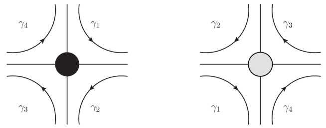
Figure 14: Base of cycles for black and white vertices.

A cycle $\alpha_{i}$ passing through the vertex $v$ can be always decomposed in sum or differences of the $\gamma^{v}_{m}$. We define the antisymmetric index $\delta_{v}$ on the $\gamma^{v}_{m}$ basis as follows

$$\delta_{v}(\gamma_{m}\wedge\gamma_{p})=-\delta_{v}(\gamma_{p}\wedge\gamma_{m})$$

$$\delta_{v}(\gamma_{m}\wedge\gamma_{m+1})=\frac{1}{2}=\delta_{v}(\gamma_{m-1}\wedge\gamma_{m})$$ (100)

$$\delta_{v}(\gamma_{m}\wedge\gamma_{n\neq m+1\&n\neq m-1})=\delta_{v}(\gamma_{m}\wedge\gamma_{m})=0$$

where a periodic enumeration of the basis, i.e. $(m+val[v]=m)$, is implicit. Now we can find the index $\delta_{v}(\alpha_{i}\wedge\alpha_{j})$ for two arbitrary cycles passing through the vertex $v$. We decompose the cycles $\alpha_{i}$ and $\alpha_{j}$ around $v$ on the base $\gamma^{v}_{m}$

$$\alpha_{i}=a_{i}^{m}\gamma^{v}_{m}\qquad\alpha_{j}=a_{j}^{m}\gamma^{v}_{m}$$ (101)

where $a_{i}^{m}$ are $0,\pm 1$ depending on the edges and on the orientation of $\alpha_{i}$ with respect to $\gamma_{v}^{m}$. Then the index is

$$\delta_{v}(\alpha_{i}\wedge\alpha_{j})=a_{i}^{m}a_{j}^{n}\delta_{v}(\gamma_{m}\wedge\gamma_{n})$$ (102)

Using these rules we can obtain the index $\delta_{v}$ at each vertex. Then summing on the common vertices as in (99), we can obtain the antisymmetric intersection pairing $\epsilon_{\alpha_{i},\alpha_{j}}$. We provide an example in Figure 15.

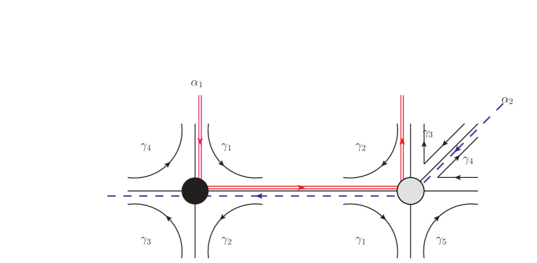
Figure 15: $\epsilon_{\alpha_{1},\alpha_{2}}=1$

In the Figure the cycle $\alpha_{1}$ is the red one (double line), and the cycle $\alpha_{2}$ is the blu one (dashed line). They can be expanded on the basis of the $\gamma_{m}$ around each vertex. The intersection is

$$\epsilon_{\alpha_{1},\alpha_{2}} = +\delta_{black}(\alpha_{1}\wedge\alpha_{2})-\delta_{white}(\alpha_{1}\wedge\alpha_{2})=$$

$$+\delta_{black}(\gamma_{1}\wedge(\gamma_{2}+\gamma_{3}))-\delta_{white}(-\gamma_{2}\wedge(-\gamma_{1}-\gamma_{4}-\gamma_{5}))=1$$

One can check that these rules reproduce the intersection numbers in Goncharov:2011hp ; Franco:2011sz ; Eager:2011dp .

Appendix B Spider move transformations

This is essentially a review section of the result of Goncharov:2011hp on Seiberg duality on the integrable dimer model. First we introduce a parametrization of the loops in terms of ratio of edges (of fields), see also Franco:2011sz ; Eager:2011dp . A loop is given by the difference of the $I$-th perfect matching and the $J$-th and we can parameterize it as in 5. Then we define a new $G+2\times n$ matrix $F$, where $n$ is the number of fields, such that $A=Fd^{T}$

$$w_{A}=e^{x_{m}B_{m,s}^{-1}F_{s,i}d_{i,A}^{T}}$$ (104)

where the sums are understood. Then we define $t_{i}=x_{m}B_{m,s}^{-1}F_{s,i}$ and (104) becomes

$$w_{A}=\prod_{i=1}^{n}e^{t_{i}d_{i,A}^{T}}$$ (105)

Then we associate to every field a factor $\phi_{i}=e^{t_{i}}$. Then the $A$ index represents the loop. By dividing $n$ in the values of its entries $n=\{n_{+},n_{-},0\}$

$$w_{A}=\frac{{\prod}_{i\in n_{+}}\phi_{i}}{{\prod}_{j\in n_{-}}\phi_{j}}$$ (106)

where $n_{+}$ and $n_{-}$ refers to the $\pm 1$ entries of the $A$-th row of the incidence matrix $d$. Now, the spider move is a local transformation on the tiling, and it corresponds to a Seiberg duality on the dual field theory. It is represented by the transformation depicted in Figure 13. The white node labelled $1,2,3,4$ are the ones connected with the rest of the tiling, which is invariant under the spider move. Hence the entire characterization of this transformation can be encoded in the modifications of the structure of the edges connecting the nodes $1,2,3,4$. We label the edges involved in the spider move as in the Figure 16.

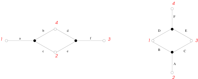
Figure 16: Details of the Spider Move

In order for the two phases to describe the same integrable system, we should match the perfect matchings in the two descriptions. A perfect matching can be decomposed in an external part, which is not modified by the spider move, and an internal part, which is made by edges connecting the various vertices. We can parametrize the internal perfect matchings in the following way. Given two external vertices $i,j$, we denote with $p_{ij}$ the internal perfect matchings which do not touch the vertices $i,j$. This parametrization can be done for the two phases of the dimer, leading to

$$p_{12}=bf,\quad\quad p_{13}=be+cd,\quad\quad p_{14}=cf$$

$$p_{23}=ad,\quad\quad p_{24}=af,\quad\quad\quad\,\,\,\,\,p_{34}=ae$$ (107)

before the transformation

$$p_{12}^{\prime}=CF,\quad\quad p_{13}^{\prime}=AF,\quad\quad\quad\quad\quad p_{14}^{\prime}=AE$$

$$p_{23}^{\prime}=BF,\quad\quad p_{24}^{\prime}=BE+CD,\quad\quad p_{34}^{\prime}=AD$$ (108)

after the the transformation. In order for the two integrable systems to be equivalent the internal perfect matchings of the two phases should be proportional one to each other Goncharov:2011hp

$$p_{ij}\sim p_{ij}^{\prime}$$ (109)

Ultimately we are interested in finding the mapping between cycles of the two phases. Cycles which do not intersect the dualized face $w_{X}$ are not modified by the spider move, and hence are identified in the two dual phases. Cycles which intersect the face $w_{X}$ are instead involved in the spider move. Such cycles can be decomposed in a basis of local path given in Figure: $\gamma_{12},\gamma_{23},\gamma_{34},\gamma_{41},w_{X}$ for phase (I) and $\gamma^{\prime}_{12},\gamma^{\prime}_{23},\gamma^{\prime}_{34},\gamma^{\prime}_{41},w^{\prime}_{X}$ for phase (II). These paths can be understood as ratio of edges

$$\gamma_{12}=\frac{a}{c},\quad\,\gamma_{23}=\frac{e}{f},\quad\,\,\gamma_{34}=\frac{f}{d},\quad\,\,\gamma_{41}=\frac{b}{a},\quad w_{X}=\frac{1}{\gamma_{12}\gamma_{23}\gamma_{34}\gamma_{41}}$$ (110)

$$\gamma^{\prime}_{12}=\frac{B}{A},\quad\gamma^{\prime}_{23}=\frac{A}{C},\quad\gamma^{\prime}_{34}=\frac{E}{F},\quad\gamma^{\prime}_{41}=\frac{F}{D},\,\,\,\,\,w^{\prime}_{X}=\frac{1}{\gamma^{\prime}_{12}\gamma^{\prime}_{23}\gamma^{\prime}_{34}\gamma^{\prime}_{41}}$$ (111)

The requirement (109) can then be translated in a map between cycles in the two dual phases. For instance

$$\gamma_{12}=\frac{p_{24}}{p_{14}}=\frac{p^{\prime}_{24}}{p^{\prime}_{14}}=\frac{BE+CD}{AE}=\gamma^{\prime}_{12}\left(1+w^{\prime}_{X}\right)$$ (112)

and so on for the other ratios of $p_{ij}$ and $p^{\prime}_{ij}$ leading to (90).

Appendix C Perfect Matchings of $Y^{30}$ and $Y^{40}$

C.1 $Y^{30}$

The quiver gauge theory, the tiling and the toric diagram for $Y^{30}$ are reported in the Figure 10. The superpotential is

$$W = X_{61}^{(1)}X_{12}X_{23}^{(2)}X_{36}-X_{61}^{(2)}X_{12}X_{23}^{(1)}X_{36}+X_{61}^{(2)}X_{14}X_{45}^{(1)}X_{56}$$ (113)

$$-X_{61}^{(1)}X_{14}X_{45}^{(2)}X_{56}+X_{23}^{(1)}X_{34}X_{45}^{(2)}X_{52}-X_{23}^{(2)}X_{34}X_{45}^{(1)}X_{52}$$

The external perfect matchings are given in Figure 17 while the internal perfect matchings are given in Figure 18.

C.2 $Y^{40}$

The quiver gauge theory, the tiling and the toric diagram for $Y^{40}$ are reported in the Figure 11. The superpotential is

$$W = X_{15}^{(1)}X_{58}X_{84}^{(2)}X_{41}-X_{15}^{(2)}X_{58}X_{84}^{(1)}X_{41}+X_{15}^{(2)}X_{56}X_{62}^{(1)}X_{21}-X_{15}^{(1)}X_{56}X_{62}^{(2)}X_{21}$$

$$+ X_{62}^{(2)}X_{23}X_{37}^{(1)}X_{76}-X_{62}^{(1)}X_{23}X_{37}^{(2)}X_{76}+X_{37}^{(2)}X_{78}X_{84}^{(1)}X_{43}-X_{37}^{(1)}X_{78}X_{84}^{(2)}X_{43}$$

The external perfect matchings are given in Figure 19 while the internal perfect matchings are given in Figure 20.

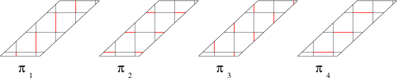
Figure 17: External perfect matching for $Y^{30}$

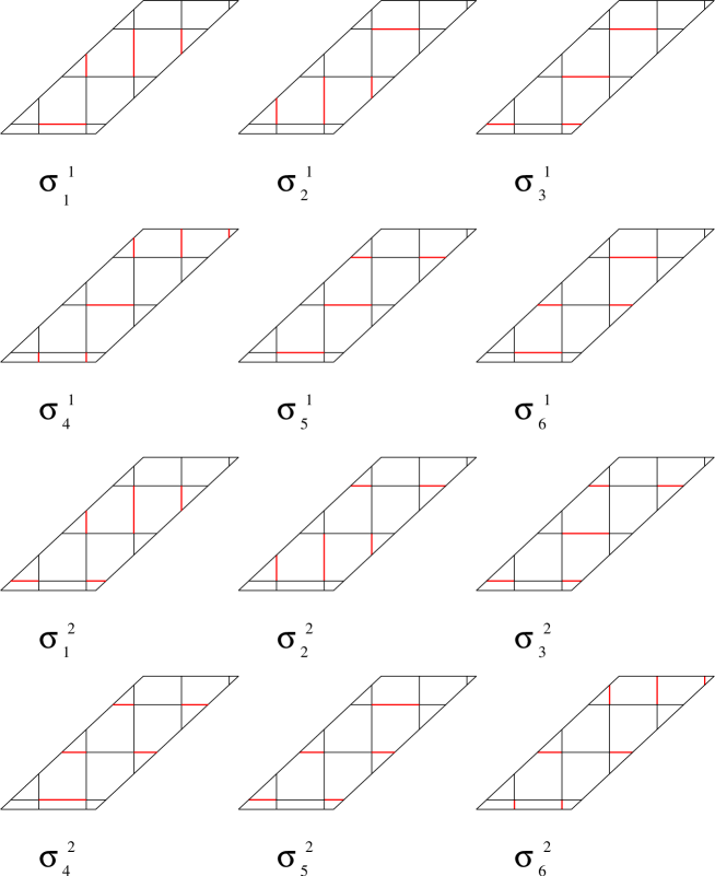
Figure 18: Internal perfect matching for $Y^{30}$

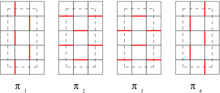
Figure 19: External perfect matching for $Y^{40}$

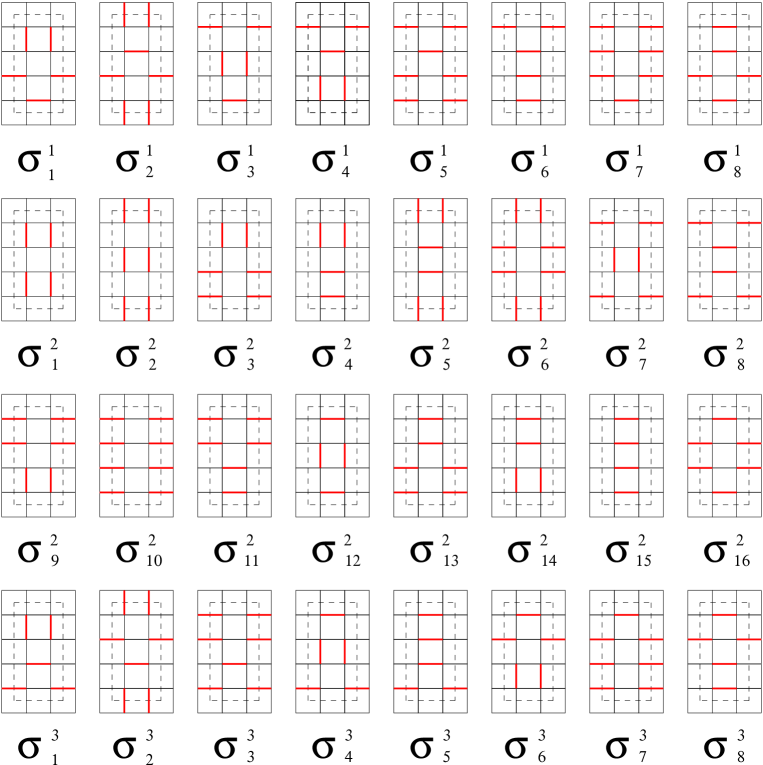
Figure 20: Internal perfect matching for $Y^{40}$

References

- (1) K. D. Kennaway, Brane Tilings, Int.J.Mod.Phys. A22 (2007) 2977–3038, [arXiv:0706.1660].
- (2) A. Hanany and K. D. Kennaway, Dimer models and toric diagrams, hep-th/0503149.
- (3) S. Franco, A. Hanany, K. D. Kennaway, D. Vegh, and B. Wecht, Brane dimers and quiver gauge theories, JHEP 0601 (2006) 096, [hep-th/0504110].
- (4) A. Hanany and D. Vegh, Quivers, tilings, branes and rhombi, JHEP 0710 (2007) 029, [hep-th/0511063].
- (5) B. Feng, Y.-H. He, K. D. Kennaway, and C. Vafa, Dimer models from mirror symmetry and quivering amoebae, Adv. Theor. Math. Phys. 12 (2008) 3, [hep-th/0511287].
- (6) A. B. Goncharov and R. Kenyon, Dimers and cluster integrable systems, arXiv:1107.5588.
- (7) V. V. Fock and A. B. Goncharov, The quantum dilogarithm and representations of quantum cluster varieties, Inventiones Mathematicae 175 (Sept., 2008) 223–286, [math/0702].
- (8) H. Derksen, J. Weyman, and A. Zelevinsky, Quivers with potentials and their representations I: Mutations, ArXiv e-prints (Apr., 2007) [arXiv:0704.0649].
- (9) S. Franco, Dimer Models, Integrable Systems and Quantum Teichmuller Space, JHEP 1109 (2011) 057, [arXiv:1105.1777].
- (10) R. Eager, S. Franco, and K. Schaeffer, Dimer Models and Integrable Systems, arXiv:1107.1244.
- (11) R. Eager and S. Franco, Colored BPS Pyramid Partition Functions, Quivers and Cluster Transformations, arXiv:1112.1132.
- (12) D. Forcella, A. Hanany, Y.-H. He, and A. Zaffaroni, The Master Space of N=1 Gauge Theories, JHEP 0808 (2008) 012, [arXiv:0801.1585].
- (13) P. Kasteleyn, Dimer statistics and phase transitions, J. Mathematical Phys. 4 (1963) 287 293.
- (14) W. Fulton, Introduction to toric varieties, Annals of Mathematics Studies, Princeton University Press 131 (1993).
- (15) A. Butti, D. Forcella, A. Hanany, D. Vegh, and A. Zaffaroni, Counting Chiral Operators in Quiver Gauge Theories, JHEP 0711 (2007) 092, [arXiv:0705.2771].
- (16) A. Weinstein, The local structure of Poisson manifold, J. Differential Geometry 18 (1983) 523–557.
- (17) B. Feng, A. Hanany, and Y.-H. He, D-brane gauge theories from toric singularities and toric duality, Nucl.Phys. B595 (2001) 165–200, [hep-th/0003085].
- (18) C. E. Beasley and M. Plesser, Toric duality is Seiberg duality, JHEP 0112 (2001) 001, [hep-th/0109053].
- (19) B. Feng, A. Hanany, Y.-H. He, and A. M. Uranga, Toric duality as Seiberg duality and brane diamonds, JHEP 0112 (2001) 035, [hep-th/0109063].
- (20) D. Forcella, A. Hanany, and A. Zaffaroni, Master Space, Hilbert Series and Seiberg Duality, JHEP 0907 (2009) 018, [arXiv:0810.4519].
- (21) S. Benvenuti, S. Franco, A. Hanany, D. Martelli, and J. Sparks, An Infinite family of superconformal quiver gauge theories with Sasaki-Einstein duals, JHEP 0506 (2005) 064, [hep-th/0411264].
- (22) S. Benvenuti and M. Kruczenski, From Sasaki-Einstein spaces to quivers via BPS geodesics: L**p,q—r, JHEP 0604 (2006) 033, [hep-th/0505206].
- (23) A. Butti, D. Forcella, and A. Zaffaroni, The Dual superconformal theory for L**pqr manifolds, JHEP 0509 (2005) 018, [hep-th/0505220].
- (24) S. Franco, A. Hanany, D. Martelli, J. Sparks, D. Vegh, et. al., Gauge theories from toric geometry and brane tilings, JHEP 0601 (2006) 128, [hep-th/0505211].
- (25) J. Propp, Generalized domino-shuffling, ArXiv Mathematics e-prints (Nov., 2001) [math/0111034].
- (26) O. Aharony, O. Bergman, D. L. Jafferis, and J. Maldacena, N=6 superconformal Chern-Simons-matter theories, M2-branes and their gravity duals, JHEP 0810 (2008) 091, [arXiv:0806.1218].
- (27) A. Hanany and A. Zaffaroni, Tilings, Chern-Simons Theories and M2 Branes, JHEP 0810 (2008) 111, [arXiv:0808.1244].
- (28) A. Hanany, D. Vegh, and A. Zaffaroni, Brane Tilings and M2 Branes, JHEP 0903 (2009) 012, [arXiv:0809.1440].
- (29) D. Martelli and J. Sparks, Moduli spaces of Chern-Simons quiver gauge theories and AdS(4)/CFT(3), Phys.Rev. D78 (2008) 126005, [arXiv:0808.0912].
- (30) S. Franco, A. Hanany, J. Park, and D. Rodriguez-Gomez, Towards M2-brane Theories for Generic Toric Singularities, JHEP 0812 (2008) 110, [arXiv:0809.3237].
- (31) D. L. Jafferis, I. R. Klebanov, S. S. Pufu, and B. R. Safdi, Towards the F-Theorem: N=2 Field Theories on the Three-Sphere, JHEP 1106 (2011) 102, [arXiv:1103.1181].
- (32) D. R. Gulotta, C. P. Herzog, and S. S. Pufu, Operator Counting and Eigenvalue Distributions for 3D Supersymmetric Gauge Theories, JHEP 1111 (2011) 149, [arXiv:1106.5484].
- (33) A. Amariti, C. Klare, and M. Siani, The Large N Limit of Toric Chern-Simons Matter Theories and Their Duals, arXiv:1111.1723.
- (34) L. Faybusovich and M. Gekhtman, Elementary Toda orbits and integrable lattices, IJ. Math. Phys. 41(5) (2000) 2905 2921.