Dynamical structure factor of quasi-2D antiferromagnet in high fields

Abstract

We study high-field magnon dynamics and examine the dynamical structure factor in the quasi-2D tetragonal Heisenberg antiferromagnet with interlayer coupling corresponding to realistic materials. Within spin-wave theory, we show that a non-zero interlayer coupling mitigates singular corrections to the excitation spectrum occurring in the high-field regime that would otherwise require a self-consistent approach beyond the $1/S$ approximation. For the fields between the threshold for decays and saturation field we observe widening of the two-magnon sidebands with significant shifting of the spectral weight away from the quasiparticle peak. We find spectrum broadening throughout large regions of the Brillouin zone, dramatic redistributions of spectral weight to the two-magnon continuum, two-peak structures and other features clearly unlike conventional single-particle peaks.

I Introduction

Studies of quantum antiferromagnets are prominent in magnetism, elucidating the role of symmetry, fluctuations and dimensionality in the ground state of many-body systems, revealing complex dynamical properties of spin excitations and allowing detailed comparison between theory and experiments.Manousakis ; Mattis ; Diep ; Johnston ; Balents ; Giamarchi08 A better understanding of many phenomena, from superfluidity to complex quantum phases may also be achieved through comparative investigations of systems of strongly interacting bosons and frustrated antiferromagnets. Balents ; Giamarchi08 ; Stone06 Recent developments in the synthesis of molecular based antiferromagnets with moderate exchange constants Woodward02 ; Lancaster07 ; Coomer07 ; Xiao09 has opened previously unreachable high magnetic field regime to experimental investigations.Tsyrulin09 ; Tsyrulin10 Furthermore, the recent completion of neutron scattering instruments with enhanced resolution Ollivier2010 ; Bewley2011 ; Ehlers2011 provides an opportunity to study the dynamics of quantum antiferromagnets in a much wider momentum-energy space and under the influence of applied magnetic field.

In a collinear antiferromagnet, e.g., a square-lattice Heisenberg antiferromagnet, magnetic field induces a non-collinearity of the magnetic order, similar to the effect of geometric frustration due to competing interactions, present in some other spin systems. J1J2J3 ; Henley Generally, non-collinearity leads to an enhanced interaction among spin excitationsChernyshev06 ; triangle and results in stark differences from conventional theory for magnons in the high-field regime.field ; Mourigal2010 ; Kreisel08 ; Syromyat09 In increasing field, spins gradually cant toward the field direction until they reach the saturation field, $H_{s}$, where quantum fluctuations are fully suppressed and ferromagnetic alignment achieved. For fields above a certain threshold value, $H^{*}$, but below saturation, coupling of the transverse and longitudinal spin fluctuations provides a channel for decays, through cubic terms in the spin-wave expansion. In this regime, magnons are predicted to be strongly damped, resulting in the loss of well-defined quasiparticle peaks.field

Magnon decays and spectrum broadening above the threshold field in the purely two-dimensional square-lattice antiferromagnet have been confirmed via quantum Monte CarloOlav08 (QMC) and exact diagonalizationLauchli09 numerical studies. In addition, QMC has revealed a non-trivial redistribution of spectral weight resulting in non-Lorentzian “double peak” features in the dynamical structure factor, also previously observed in the original analytical study.field The inelastic neutron-scattering experiment on the spin-$5/2$ material $\rm{Ba_{2}MnGe_{2}O_{7}}$ are also indicative of the field-induced magnon decays,Masuda10 although not fully conclusive.Mourigal2010 It can be argued that recent thermal conductivity experiments in the so-called Bose-Einstein condensed magnets that observed suppression of heat current in the vicinity of critical fieldsKohama2011 are related to magnon decay dynamics.sasha_unpub Current advances in neutron scattering instrumentationOllivier2010 ; Bewley2011 ; Ehlers2011 open avenues to search for decays in large portions of the (${\bf k},\omega$) space. This is a particularly important issue in the case of spin-$1/2$ systems for which a comparison of experimental findings with existing theories is still missing.

In this work, we extend the previous work of three of us and provide a theoretical investigation of high-field dynamics in the quasi-2D tetragonal $S\!=\!1/2$ Heisenberg antiferromagnet with interlayer coupling corresponding to realistic materials. In particular, within spin-wave theory in the $1/S$ approximation, we obtain quantitative predictions for the dynamical structure factor, $S({\bf k},\omega)$, the quantity measured in inelastic neutron scattering experiments, for a representative interlayer coupling ratio $J^{\prime}/J\!=\!0.2$, relevant, e.g., for $\rm{(5CAP)_{2}CuCl_{4}}$,Coomer07 along several representative paths in the Brillouin zone and for magnetic fields of $H\!=\!0.90H_{s}$ and $H\!=\!0.95H_{s}$.

Within the framework of spin-wave theory, 3D coupling also helps with the following technical issues. First, in the case of the 2D, $S\!=\!1/2$ square-lattice antiferromagnet in high fields, calculations without the self-consistent treatment of cubic magnon interactions lead to renormalized quasiparticle peaks that unrealistically escape the (unrenormalized) two-magnon continuum, precluding an accurate determination of the dynamical structure factor.field Second, for the same 2D case, the standard $1/S$ expansion for the magnon spectrum breaks down in the high-field regime, owing to the transfer of the van Hove singularities from the two-magnon continuum to the one-magnon mode due to a coupling between the two.field ; Mourigal2010 To regularize such unphysical singularities, two self-consistent schemes were developed in Refs. field, and Mourigal2010, . While the former approachfield did take into account the renormalization of the spectrum and, as a consequence, the spectral weight redistribution, it was only partially self-consistent. The latter, on the other hand, ignored the real part of the spectrum renormalization,Mourigal2010 essentially enforcing Lorentzian shapes of the quasiparticle peaks and excluding more complex profiles such as “double-peak” features.field ; Olav08 While this latter approach is suitable for spins $S\!\geq\!1$,Mourigal2010 it cannot be deemed satisfactory in the case of $S\!=\!1/2$.

The aim of this work is to demonstrate that a non-zero 3D interlayer coupling largely mitigates the singularities of high-field corrections and thus provides a physical representation of the excitation spectrum without the use of self-consistency. While the quasiparticle energy shift and corresponding escape from the “bare” continuum are still present to some degree within this approach, they are considerably weaker than in the purely 2D case, allowing for a detailed analysis of the effects of broadening and weight redistribution in the spectrum. Altogether, the relatively simple $1/S$ approximation requires considerably less computation than self-consistent methods, follows the spirit of the regular spin-wave expansion and allows quantitative examination of the dynamical structure factor. This approach is applicable to all spin values including the spin-$1/2$ case, which is the focus of our study. Since all real antiferromagnets are at best quasi-two-dimensional, our analysis is relevant to most realistic materials, even those with weak interlayer coupling. Results of the present work therefore consist in detailed and clear predictions for the dynamical structure factor to guide experiments and a comparison with self-consistent techniques for the purely 2D case.

The paper is organized as follows: Section II contains an overview of the spin-wave formalism, with full details in Appendix A. Following in Section III is a brief discussion of decay conditions and singularities. Section IV contains the dynamical structure factor calculated in the $1/S$ approximation for non-zero interlayer coupling. Section V contains our conclusions. Appendix A contains details of the $1/S$ spin-wave theory for the quasi-2D tetragonal Heisenberg antiferromagnet in external field.

II Interacting Spin Waves in Field

We begin with the Heisenberg Hamiltonian of nearest-neighbor interacting spins on a tetragonal lattice in the presence of an applied magnetic field directed along $z_{0}$ axis in the laboratory reference frame,

$$\hat{\cal H}=\sum_{\langle ij\rangle}J_{ij}\ \mathbf{S}_{i}\cdot\mathbf{S}_{j}-H\sum_{i}S_{i}^{z_{0}}\ ,$$ (1)

where in-plane coupling is $J_{ij}\!=\!J$ and the interplane one is $J_{ij}\!=\!J^{\prime}\!=\!\alpha J$ and we assume $0\!\leq\!\alpha\!\leq\!1$. With the details of the technical approach explicated in Appendix A and Refs. Nikuni98, ; field, ; Mourigal2010, , we summarize here the key steps of the spin-wave theory approach to this problem.

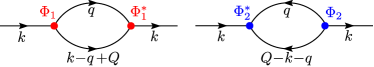
Figure 1: (Color online) Self-energies in the lowest $1/S$ order obtained from decay (left) and source (right) interactions.

First, we identify the canted spin configuration in the equivalent classical spin model. Then we quantize the spin components in the rotating frame that aligns the local spin quantization axis on each site in the direction given by such a classical configuration. Application of the standard Holstein-Primakoff transformation bosonizes spin operators. After subsequent Fourier transformation, the Hamiltonian is diagonalized via the Bogoliubov transformation, yielding the Hamiltonian that can be written astriangle

$$\hat{\cal H}=\sum_{\bf k}\tilde{\varepsilon}_{\bf k}b_{\bf k}^{\dagger}b_{\bf k}^{\phantom{\dagger}} + \frac{1}{2!}\sum_{\bf k,q}\Phi_{1}({\bf k,q})\bigl{(}b_{\bf k-q+Q}^{\dagger}b_{\bf q}^{\dagger}b_{\bf k}^{\phantom{\dagger}}+\rm{h.c.}\bigr{)}$$

$$+ \frac{1}{3!}\sum_{\bf k,q}\Phi_{2}({\bf k,q})\bigl{(}b_{\bf Q-k-q}^{\dagger}b_{\bf q}^{\dagger}b_{\bf k}^{\dagger}+\rm{h.c.}\bigr{)}+...$$

where the ordering vector ${\bf Q}=(\pi,\pi,\pi)$ enters the momentum conservation condition because of the staggered canting of spins.Mourigal2010 In this expression, $\tilde{\varepsilon}_{\bf k}=\varepsilon_{\bf k}+\delta\varepsilon_{\bf k}$, where $\varepsilon_{\bf k}$ is the “bare” magnon dispersion given by linear spin-wave theory and $\delta\varepsilon_{\bf k}$ contains $1/S$ corrections from angle renormalization and Hartree-Fock decoupling of cubic and quartic perturbations, respectively. Ellipses stand for higher-order terms in the $1/S$ expansion that are neglected in our approximation. The three-boson terms are decay and source vertices that are responsible for the anomalous dynamics in the high-field regime. The dynamical properties of the system are obtained from the interacting magnon Green’s function, defined as

$$G^{-1}({\bf k},\omega)=\omega-\tilde{\varepsilon}_{\bf k}-\Sigma_{1}({\bf k},\omega)-\Sigma_{2}({\bf k},\omega)$$ (3)

where $\Sigma_{1,2}({\bf k},\omega)$ are the decay and source self-energies presented in Fig. 1 and obtained from the second-order treatment of Eq. (II). Their explicit forms are

$$\Sigma_{1}({\bf k},\omega) = \frac{1}{2}\sum_{\bf q}\frac{|\Phi_{1}({\bf k},{\bf q})|^{2}}{\omega-\varepsilon_{\bf q}-\varepsilon_{\bf k-q+Q}+i0}\ ,$$ (4)

$$\Sigma_{2}({\bf k},\omega) = -\frac{1}{2}\sum_{\bf q}\frac{|\Phi_{2}({\bf k},{\bf q})|^{2}}{\omega+\varepsilon_{\bf q}+\varepsilon_{\bf k+q-Q}-i0}\ ,$$ (5)

with expressions for vertices $\Phi_{1}$ and $\Phi_{2}$ given in Appendix A. In contrast to $H\!=\!0$ case where $\omega$-dependent magnon interactions beyond Hartree-Fock have $1/S^{2}$ smallness, they readily occur in $1/S$ order for $H\neq 0$, when the coupling between longitudinal and transverse modes renders three-boson vertices nonzero. Above the threshold field for magnon instability, the self-energy in (4) also acquires an imaginary component, signifying the occurrence of spontaneous decays.

III Kinematics, singularities and interlayer coupling

III.1 Decay boundaries

Although the single- and two-magnon continuum excitations are coupled directly by virtue of the cubic terms in Eq. (II) at any $H>0$, magnon decays only occur above a finite threshold field $H^{*}$. This is due to restrictions provided by the kinematic conditions, i.e., energy and momentum conservation, that have to be satisfied in each elementary decay process

$$\varepsilon_{\bf k}=\varepsilon_{\bf q}+\varepsilon_{\bf k-q+Q},$$ (6)

where the ordering vector in the momentum conservation is, again, due to the staggered canting of spins in the field.

With the detailed classification of possible solutions of Eq. (6) given previously in Refs. triangle, ; Mourigal2010, we highlight here two relevant results. First, it can be shown that within the Born approximation, that is, neglecting energy renormalization of the spectrum $\varepsilon_{\bf k}$ from the linear spin-wave theory result, the value of the threshold field $H^{*}$ is independent of the value of the interlayer coupling $\alpha$ and is the same as in the square lattice case: $H^{*}\!\approx\!0.76H_{s}$.

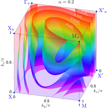
Figure 2: (Color online) Magnon decay regions in one octant of the Brillouin zone for several fields. Decays are possible within the portion of the Brillouin zone containing the $\rm{M}_{\pi}$ point. At high fields, decay regions extend beyond the octant and overlap, facilitating larger phase space for decays for magnons within the decay region.

Second, for a given field $H>H^{*}$, within the same Born approximation that neglects cascade decays, there exists a sharp boundary in the momentum space separating the region where magnons are stable, i.e., cannot satisfy Eq. (6), from the decay region where they are unstable towards decays. An example of such decay boundaries in a 3D setting is shown in Fig. 2 in one octant of the tetragonal-lattice Brillouin zone for $\alpha=0.2$ and several fields.footnote One can see that the decay region expands with increasing field, covering large portions of the Brillouin zone. At high fields, decay regions extend beyond the octant and overlap; at $H\gtrsim 0.9H_{s}$ most magnons are unstable already in the Born approximation.

Taking into account the finite lifetime of the decay products in the self-consistent treatment generally leads to blurring away the decay boundaries discussed here.field ; Mourigal2010 Nevertheless, it is still important to consider them not only because the decays within the Born decay region typically remain more intense as they occur in the lower-order process, but also because such boundaries correspond to singularities in the spectrum discussed next.footnote1

III.2 On-shell approximation

Within the standard spin-wave expansion, the on-shell approximation for the magnon spectrum consists of setting $\omega=\varepsilon_{\bf k}$ in the self-energies in Eqs. (4), (5), leading to the renormalized spectrum

$$\bar{\varepsilon}_{\bf k}=\tilde{\varepsilon}_{\bf k}+{\rm Re}\,\Sigma_{1}({\bf k},\varepsilon_{\bf k})+\Sigma_{2}({\bf k},\varepsilon_{\bf k}),$$ (7)

and the decay rate

$$\Gamma_{\bf k}=\frac{\pi}{2}\sum_{\mathbf{q}}|\Phi_{1}(\mathbf{k,q)}|^{2}\delta\bigl{(}\varepsilon_{\bf k}-\varepsilon_{\bf q}-\varepsilon_{\bf k-q+Q}\bigr{)}.$$ (8)

We note that this approach implicitly suggests that the dynamical response can be well approximated by the quasiparticle peaks at renormalized energies $\bar{\varepsilon}_{\bf k}$ with lorentzian broadening defined by $\Gamma_{\bf k}$. As was demonstrated in Ref. field, ; Mourigal2010, for the 2D square-lattice and in Ref. triangle, for the triangular-lattice cases, this approach, which is normally very accurate even quantitatively, breaks down rather dramatically, showing divergences in $\bar{\varepsilon}_{\bf k}$ or $\Gamma_{\bf k}$ for the momenta belonging to various contours in ${\bf k}$-space. We reproduce some of them in our Fig. 3, shown by dashed lines. These singularities were understood as coming from the van Hove singularities in the two-magnon continuum through coupling with the single-magnon branch. One can see in the expression for $\Gamma_{\bf k}$ in Eq. (8) that once the continuum and the single-magnon branch overlap in some portion of the Brillouin zone, $\varepsilon_{\bf k}$ is effectively exploring the two-magnon density of states as a function of ${\bf k}$. If a singularity in the latter is met, it will be reflected in $\Gamma_{\bf k}$ and, by the Kramers-Kronig relation, in $\bar{\varepsilon}_{\bf k}$.

Generally, there are two types of singularities that can occur, associated with the minima (maxima) and saddle points of the two-magnon continuum, respectively. The decay boundaries discussed previously are necessarily the surfaces of such singularities because they must correspond to the intersection with a minimum of the two-magnon continuum, forming the locus of points where decay conditions are first met. These decay threshold singularities correspond to the step-like behavior in $\Gamma_{\bf k}$ and the logarithmic divergence in $\bar{\varepsilon}_{\bf k}$.field ; triangle ; Mourigal2010 For the ${\bf k}$-points already inside the decay region, there is a possibility of meeting a saddle point of the continuum, in which case the real part of the spectrum $\bar{\varepsilon}_{\bf k}$ experiences a jump and $\Gamma_{\bf k}$ a logarithmic singularity, see the 2D data in Fig. 3.

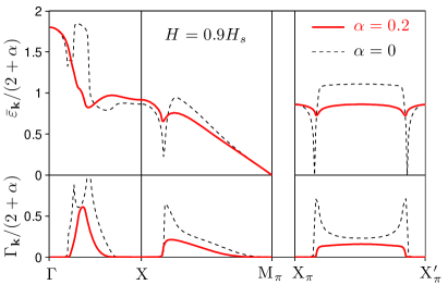
Figure 3: (Color online) Magnon energy and decay rate for $\alpha=0.2$ and for the square-lattice case ($\alpha=0$) for $H=0.9H_{s}$ along the selected path in the Brillouin zone (see Fig. 7). Upper and lower panels show the renormalized spin-wave energy $\bar{\varepsilon}_{\bf k}$ and the decay rate $\Gamma_{\bf k}$ in the on-shell approximation, Eqs. (7) and (8), respectively. Computation was performed with Monte-Carlo numerical integration with $5\cdot 10^{7}$ steps.

Essential for the present study is the change in the behavior of these singularities for a moderate interlayer coupling. One can expect from the density of states argument that both types of singularities must become weaker and change from logarithmic/step-like to square-root-like,triangle resulting in softening of the singular behavior of $\Gamma_{\bf k}$ and $\bar{\varepsilon}_{\bf k}$. This effect is demonstrated in Fig. 3 for several directions in the 3D Brillouin zone compared with equivalent cuts for the square-lattice case. The full account of analytical and numerical details of the on-shell calculations is given in Appendix A. The definitions concerning the Brillouin zone path in Fig. 3 can be found in Fig. 7. It is rather remarkable that the singularity of the saddle-point type is completely wiped out by the moderate interplane coupling, see panel $\Gamma-\rm{X}$ in Fig. 3. While the decay threshold singularities associated with the boundaries in Fig. 2, are not fully alleviated, they are considerably diminished. For both types of singularities, further increase of the interplane coupling leads to gradual changes in the on-shell spectrum and decay rates; singularities shown in Fig. 3 for $\alpha=0.2$ remain largely unchanged.

While singularities are diminished, the magnon damping remains considerable. Since both the decay boundaries and $\Gamma_{\bf k}$ are obtained within the Born approximation, the decay rate in Fig. 3 is non-zero within the corresponding decay region outlined in Fig. 2 for $H=0.9H_{s}$, demonstrating that magnons are unstable in most of the Brillouin zone, while the Goldstone mode at $M_{\pi}$ $[{\bf k}\!=\!(\pi,\pi,\pi)]$ and the uniform precession mode at $\Gamma$ $[{\bf k}\!=\!(0,0,0)]$ remain well-defined.

Previous works on regularization of singularities in the spin-wave spectrum in the 2D square-lattice casefield ; Mourigal2010 were based on partial dressings of magnon Green’s functions in the one-loop diagrams of Fig. 1. Generally, the difficulty of a consistent implementation of such schemes is the opening of an unphysical gap in the acoustic branch. The latter problem was avoided in Ref. Mourigal2010, by performing self-consistency only in the imaginary part of the magnon self-energy, applicable for larger $S\!\geq\!1$ where the real part of renormalization can be deemed small. The downside of this approach is that it remains essentially on-shell, enforcing Lorentzian shapes of the quasiparticle peaks. In a sense, what is being argued by our Fig. 3 is that introducing finite interplanar coupling represents an alternative to the self-consistency schemes in regularizing singularities, without restrictions on the spectral shapes and at a fraction of the computational cost.

III.3 Spectral function

The one-loop self-energies $\Sigma_{1,2}({\bf k},\omega)$ in Eqs. (4) and (5) originate from the coupling to the two-magnon continuum. Because of their $\omega$-dependence, one can obtain significantly richer dynamical information, beyond the quasiparticle pole-like state expected from the on-shell approach above, by considering the diagonal component of the spectral function,

$${A}({\bf k},\omega)=-\frac{1}{\pi}\,{\rm Im}\,G({\bf k},\omega),$$ (9)

where $G({\bf k},\omega)$ is the interacting magnon Green’s function defined in Eq. (3). Because of the interactions, the spectral function is expected to exhibit an incoherent component which should reflect the two-magnon continuum states in addition to a quasiparticle peak that may be broadened. The spectral function is directly related to the dynamical structure factor $S({\bf k},\omega)$ measured in neutron-scattering experiments, which we discuss in detail in the next Section. Strictly speaking, the consideration of $A({\bf k},\omega)$ goes beyond the $1/S$ expansion as $\omega\neq\varepsilon_{\bf k}$, yet it is free from the complications due to higher-order diagrams mentioned above.

We should note that in the pure 2D, $S=1/2$ case, non-selfconsistent calculation of $A({\bf k},\omega)$ does exhibit incoherent subbands,field but suffers from the high density of states of the two-magnon continuum associated with the threshold singularities considered above. Because of level repulsion, the renormalized quasiparticle peaks escape the unrenormalized two-magnon continuum and preclude an accurate determination of the dynamical structure factor, except for fields in close vicinity of the saturation field where the renormalization becomes weaker. However, this is not the case in the triangular-lattice antiferromagnet in zero field,triangle where the thresholds are controlled by the emission of the Goldstone magnons associated with much smaller density of states.

Similar to the weakening of the threshold singularities in 3D, one can expect weaker repulsion between the single-magnon branch and the minima of the two-magnon continuum. As will be shown in the next Section, while the quasiparticle energy shift and corresponding escape from the continuum are still present to some degree, they are considerably smaller than in the 2D case. Therefore, once again, introducing finite interplanar coupling provides an alternative to the self-consistency schemes, allowing for a detailed analysis of the effects of broadening and weight redistribution in the spectrum.

IV Dynamical Structure Factor

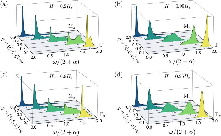
Figure 4: (Color online) Profiles of the perpendicular component of the dynamical structure factor $S_{\perp}({\bf k},\omega)$, Eq. (12), vs $\omega$ for selected ${\bf k}$-points along the main diagonal of the Brillouin zone (from $\Gamma$ to ${\rm M}_{\pi}$), panels (a) and (b), and along the diagonal in the $k_{z}=\pi$ plane (from $\Gamma_{\pi}$ to ${\rm M}_{\pi}$), (c) and (d), for fields $0.9H_{s}$ and $0.95H_{s}$, and $S=1/2$. For high-symmetry ${\bf k}$-points notations, see Figs. 2 and 7. Dashed lines indicates the linear spin-wave dispersion $\varepsilon_{\bf k}$ along the same paths.

The inelastic neutron-scattering cross section is proportional to a linear combination of the components of the spin-spin dynamical correlation functionSquires

$$S^{\alpha\beta}({\bf k},\omega)=\int_{-\infty}^{\infty}\frac{dt}{2\pi}\,\left\langle S^{\alpha}_{\bf k}(t)S^{\beta}_{-\bf k}\right\rangle\,e^{i\omega t}$$ (10)

where $\alpha,\beta=\{x_{0},y_{0},z_{0}\}$ span the Cartesian directions of the laboratory frame. For simplicity, in the following discussion we ignore additional momentum-dependent polarization factors from experimental details, on which coefficients of such linear combination can depend on, and show our results for what we will refer to as the “full” dynamical structure factor

$$S({\bf k},\omega)=S^{x_{0}x_{0}}({\bf k},\omega)+S^{y_{0}y_{0}}({\bf k},\omega)+S^{z_{0}z_{0}}({\bf k},\omega),$$ (11)

as well as its component perpendicular to the external field, the latter is directed along the $z_{0}$-axis as before,

$$S_{\perp}({\bf k},\omega)=S^{x_{0}x_{0}}({\bf k},\omega)+S^{y_{0}y_{0}}({\bf k},\omega).$$ (12)

The choice of these particular examples is both illustrative and general, as it exposes all the essential components of $S({\bf k},\omega)$.

The dynamical structure factor is naturally written in a laboratory reference frame while the magnon operators were introduced in the rotating frame that aligns local spin quantization axis on each site in the direction given by a classical configuration of spins canted in a field. Thus, the relation of the magnon spectral function, $A({\bf k},\omega)$ of Eq. (9), to $S({\bf k},\omega)$ for canted spin structures is via a two-step transformation: rotation of spins from laboratory to local frame and bosonization of spin operators.Mourigal2010 In the lowest $1/S$-order, this procedure becomes rather straightforward since most complications such as off-diagonal terms in the spin Green’s functions can be justifiably dropped as they only contribute in the order $1/S^{2}$ or higher. With that, performing the second transformation first, components of the dynamical structure factor in the local quantization frame are readily given byMourigal2010

$$S^{xx}({\bf k},\omega) \approx \pi S\Lambda_{+}\>(u_{\bf k}+v_{\bf k})^{2}A({\bf k},\omega),$$

$$S^{yy}({\bf k},\omega) \approx \pi S\Lambda_{-}\>(u_{\bf k}-v_{\bf k})^{2}A({\bf k},\omega),$$ (13)

$$S^{zz}({\bf k},\omega) \approx \pi\sum_{\bf q}(u_{\bf q}v_{\bf k-q}+v_{\bf q}u_{\bf k-q})^{2}\delta(\omega-\varepsilon_{\bf q}-\varepsilon_{\bf k-q}),$$

where $x,y,z$ now refer to local axes, $u_{\bf k}$ and $v_{\bf k}$ are parameters of the Bogoliubov transformation, and $\Lambda_{\pm}\!=\!(1\!-\!(2n\!\pm\!\delta)/2S)$ contain the $1/S$ corrections from the Hartree-Fock spin reduction factors, see Appendix A.

Strictly speaking, in these expressions for the diagonal terms of $S^{\alpha\alpha}$ we have kept contributions in excess of the leading order of $1/S$ expansion, as both the Hartree-Fock corrections to $S^{xx}$ and $S^{yy}$ as well as the $S^{zz}$ term itself are of higher order. In addition to being easy to include them into our consideration, they also offer us an opportunity to demonstrate their relative unimportance. Thus, the longitudinal component $(S^{zz})$ in the given order contains a “direct” contribution of the two-magnon continuum to the structure factor. Apart from being broadly distributed over the $({\bf k},\omega)$ space compared to a more sharply concentrated $A({\bf k},\omega)$, its contribution to the scattering turned out to be diminishingly small compared to the two transverse components $S^{xx(yy)}$ in the considered high-field regime. Besides being an effect of the higher $1/S$ order, this is also due to its dependence on $v^{2}$ ($\propto\!\cos^{4}\theta\!\ll\!1$), where $\theta$ is the spins’ canting angle which tends to $\pi/2$ as the saturation field is approached.

Completing the connection of the local form of correlation functions to the laboratory ones gives the final relation of $A({\bf k},\omega)$ to $S({\bf k},\omega)$

$$S^{x_{0}x_{0}}({\bf k},\omega) \approx \sin^{2}\!\theta\,S^{xx}({\bf k},\omega)+\cos^{2}\!\theta\,S^{zz}({\bf k}-{\bf Q},\omega)\,,$$

$$S^{z_{0}z_{0}}({\bf k},\omega) \approx \cos^{2}\!\theta\,S^{xx}({\bf k}-{\bf Q},\omega)+\sin^{2}\!\theta\,S^{zz}({\bf k},\omega)\,,$$

$$S^{y_{0}y_{0}}({\bf k},\omega) = S^{yy}({\bf k},\omega)\ ,$$ (14)

where the cross-terms in spin-spin correlation function ($S^{xz}$ and $S^{zx}$) in the r.h.s. were omitted under the same premise of not contributing in the lowest order. These last expressions demonstrate that due to external field, spin-canting redistributes the spectral weight over two transverse modes,Birgeneau ; Mourigal2010 referred to as the “in-plane” and the “out-of-plane” modes, corresponding to the momentum ${\bf k}$ and to the momentum ${\bf k}-{\bf Q}$ (and to fluctuations in and out of the plane perpendicular to applied field), respectively. As can be expected form the pre-factor $\cos^{2}\theta$ in Eq. (14), strong magnetic field suppresses the out-of-plane mode until it disappear entirely at $H_{s}$. In the $S({\bf k},\omega)$ plots that will follow, the out-of-plane contribution appears as a “shadow” of the main signal, shifted by the ordering vector.

From Eqs. (14) and (13) one can see that our choice of the perpendicular component of the structure factor $S_{\perp}({\bf k},\omega)$ in Eq. (12) as a representative example becomes particularly simple. Since it is not contaminated by the ${\bf k}-{\bf Q}$ shadow component and the contribution of the longitudinal $S^{zz}({\bf k},\omega)$ to it is exceedingly small in the considered field range, it is closely approximated by

$$S_{\perp}({\bf k},\omega)\approx\pi Sf_{\bf k}A({\bf k},\omega),$$ (15)

where $f_{\bf k}\!=\!\left[\sin^{2}\!\theta\Lambda_{+}\>(u_{\bf k}\!+\!v_{\bf k})^{2}\!+\!\Lambda_{-}\>(u_{\bf k}\!-\!v_{\bf k})^{2}\right]$ is the ${\bf k}$- and field-dependent intensity factor.

Our Fig. 4 presents the perpendicular component of the dynamical structure factor $S_{\perp}({\bf k},\omega)$ for $S\!=\!1/2$, fields of $0.9H_{s}$ and $0.95H_{s}$, and for several ${\bf k}$-points along two representative directions: main diagonal of the Brillouin zone (from $\Gamma$ to ${\rm M}_{\pi}$), Fig. 4(a) and (b), and diagonal of the $k_{z}=\pi$ plane (from $\Gamma_{\pi}$ to ${\rm M}_{\pi}$), Fig. 4(c) and (d), respectively. To obtain these profiles, integrals in the self-energies in Eqs. (4) and (5) and in $S^{zz}({\bf k},\omega)$ in Eq. (13) were computed using Mathematica via adaptive quasi-Monte-Carlo without symbolic preprocessing, over $5\cdot 10^{6}$ points, maximum recursion of $10^{4}$, and an accuracy goal of 4 digits. Each presented ${\bf k}$-cut contains 400 points in $\omega$ and an artificial broadening $\delta/(2\!+\!\alpha)=10^{-2}J$ was used. As we discussed, contribution of the longitudinal term $S^{zz}$ is not visible on the scale of the plots. Dashed lines show linear spin-wave dispersions for the given paths.

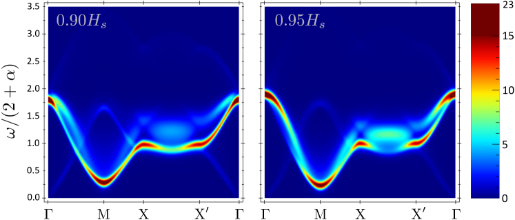
Figure 5: (Color online) Intensity plots of the dynamical structure factor $S({\bf k},\omega)$, Eq. (11), for fields $0.9H_{s}$ and $0.95H_{s}$, and $S=1/2$, for the ${\bf k}$-path in the $k_{z}\!=\!0$ plane, see Fig. 7. Gaussian convolution was performed in $\omega$ with a $\sigma$-width of $\delta\omega\!=\!0.1J$.

These $S_{\perp}({\bf k},\omega)$ profiles demonstrate that the spectrum broadening due to magnon decays in the high-field regime is found abundantly throughout the Brillouin zone. In addition, clear double-peak structures, similar to that seen in the self-consistent spin-wave calculationsfield and emphasized in the QMC studyOlav08 for the 2D square-lattice case, occur along the main diagonal, Fig. 4(a), (b). At $H\!=\!0.90H_{s}$, some sharp magnon peaks remain in the vicinity of the $\Gamma$-point, in agreement with the decay boundaries in Fig. 2. Peaks also get narrower at the approach of the Goldstone ${\rm M}_{\pi}$ point. Although there seems to be some sharpness in the structure of $S_{\perp}({\bf k},\omega)$ data for $H\!=\!0.90H_{s}$ in the middle of the diagonals, these are not associated with quasiparticle peaks, but with the remaining singular behavior of the one-loop self-energies.

A noteworthy feature of the shown results is a strong field-evolution of $S_{\perp}({\bf k},\omega)$, demonstrating a rather dramatic redistribution of spectral weight between the broadened single-particle and incoherent part of the spectrum, related to the two-magnon continuum. Another important observation is the relative smallness of the energy shift of the spectral-function leading edge in $\omega$ compared to the linear spin-wave energy $\varepsilon_{\bf k}$, shown by the dashed lines. This, together with a close similarity of the shown non-selfconsistent results to the self-consistent ones in the 2D square-lattice case,field is an indication of the reliability of current approach, thus supporting our expectation that presented results should serve as a fair representation of the realistic structure factor.

In Figs. 5 and 6, intensity plots of the full dynamical structure factor, $S({\bf k},\omega)$ in Eq. (11), for $S\!=\!1/2$, fields of $0.9H_{s}$ and $0.95H_{s}$, and for several representative paths in the Brillouin zone are shown. In Fig. 5, the ${\bf k}$-path is entirely in the $k_{z}=0$ plane and in Fig. 6 the momentum traces an inter-layer path, both shown in Fig. 7. As we have discussed above, in addition to the main features demonstrated in Fig. 4 for $S_{\perp}({\bf k},\omega)$ that are directly related to the magnon spectral function $A({\bf k},\omega)$, the out-of-plane transverse mode contribution is visible as a shadow, shifted by the ordering vector. The longitudinal ($S^{zz}$) contributions are hardly noticeable on the scale of the plots as before. In Fig. 6, proximity to the Goldstone mode at $M_{\pi}$ causes unphysical divergences, amplified by the divergent intensity factor $f_{\bf k}$ in Eq. (15), that necessitate removal of this region in the plot.

Integrals in the self-energies for these plots were computed by the same method as in Fig. 4, over a maxium number of points of $2\cdot 10^{5}$, with the same accuracy goal of 4 digits. There are 150 points along each segment in the ${\bf k}$-path, each with 350 points in $\omega$. All integrations were performed in parallel over 8 logical threads. The same upper cut-off in intensity has been used in both plots with additional red color fill up to the extent of the highest peak, whose value is shown in the color sidebars. Additionally, we have performed Gaussian convolution in the $\omega$-direction with a $\sigma$-width of $\delta\omega\!=\!0.1J$. This step is intended to mimic the effect of a realistic experimental resolution, from which we can also draw quantitative predictions of the relative strength of the quasiparticle and incoherent part of the spectrum.

Despite the provided broadening by the finite energy resolution, complex spectral lineshapes, very much distinct from the conventional quasiparticle peaks, are clearly visible in Figs. 5 and 6. This demonstrates that the effects of spectral weight redistribution and broadening due to spontaneous decays are substantial and should be readily observed in experiment.

Since $\Gamma$, $\rm{M}$, $\rm{X}$, and $\rm{X}^{\prime}$ points in Fig. 5 and $\Gamma$, $\rm{X}$, and $\rm{X}^{\prime}_{\pi}$ points in Fig. 6 are outside of the Born approximation decay regions according to Fig. 2, spectrum in their vicinities exhibits well-defined quasiparticle peaks, broadened by our “instrumental” resolution. However, away from them, the structure factor demonstrates a variety of unusual features, including the already discussed double-peak lineshape for $\Gamma\rm{M}$ direction in Fig. 5 and $\Gamma\rm{M}_{\pi}$ direction in Fig. 6, the latter path also shown in $S_{\perp}({\bf k},\omega)$ previously.

Along some of the ${\bf k}$-directions for $H=0.9H_{s}$ in both Fig. 5 and  6, the renormalized quasiparticle peaks escape the unrenormalized two-magnon continuum and survive despite being formally within the decay region. Yet, these peaks are accompanied by continuum-like subbands that accumulate significant weight. Upon increase of the field, the continuum overtakes the single-particle branches in the large regions of the Brillouin zone, washing them out and creating more double-peak structures, e.g., very distinctly along the $\rm{X}^{\prime}\Gamma$ (Fig. 5) and $\rm{X}^{\prime}_{\pi}\Gamma$ (Fig. 6) directions. There is a particularly spectacular advance of the continuum along the $\rm{XX}^{\prime}$ line in Fig. 5, where magnon broadening is most intense with dramatic spectral weight transfer to high-energies.

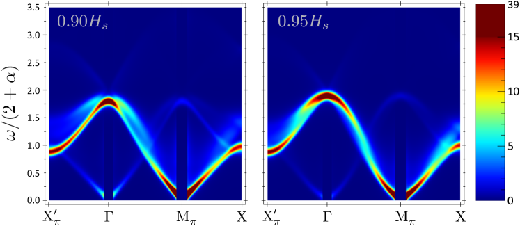
Figure 6: (Color online) Same as in Fig. 5, for a different path, see Fig. 7. The region near $\rm{M}_{\pi}$ in ${\bf k}$ and ${\bf k}-{\bf Q}$ modes are cut due to spurious divergences, see text. Note the higher cutoff in intensity due to a formfactor divergent at $\rm{M}_{\pi}$-point.

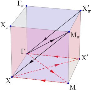
Figure 7: (Color online) Brillouin zone octant showing the ${\bf k}$-paths traversed in Figs. 5 and 6. Path in Fig. 5 lies in the $k_{z}=0$ plane and goes along the dotted line: $\rm{\Gamma}\rightarrow\rm{M}\rightarrow\rm{X}\rightarrow\rm{X^{\prime}}\rightarrow\Gamma$. Path in Fig. 6 goes between the $k_{z}=0$ and $k_{z}=\pi$ planes along the zig-zag solid line: $\rm{X^{\prime}}_{\pi}\rightarrow\rm{\Gamma}\rightarrow\rm{M}_{\pi}\rightarrow\rm{X}$.

We note that the regions where decays are present in the on-shell solutions discussed in Sec. III often correspond closely to the “washout” regions of the intensity plots, although the latter draw a much richer picture by exposing a complex $\omega$-structure. The remaining 3D singularities in the real part of the on-shell energy, exemplified in Fig. 3, indicate where the two-magnon continuum overlaps with the single-magnon branch, also in a qualitative agreement with the intensity plots, thus providing a complimentary information. Previous examination of the 2D square-lattice case in Ref. Mourigal2010, showed broadening patterns similar to the ones in Figs. 5 and Fig. 6 for corresponding paths of the Brillouin zone, although the $\omega$-structure differs significantly as the self-consistent approach of that work has enforced the Lorentzian shapes of the spectral function.

The one-loop approximation used in this work takes into account the real part of the self-energy corrections, allowing the renormalized single-magnon branch to escape some of the decay region. Therefore, the obtained dynamical structure factor is likely to overestimate the field values needed to reach a significant overlap between the two-magnon continuum and the single magnon mode throughout the Brillouin zone.

Altogether, examination of the dynamical structure factor reveals rich features consisting of dramatic redistributions of magnon spectral weight. This ranges from the appearance of double-peak lineshapes to a full suppression of quasiparticle peaks throughout large portions of the Brillouin zone. These features fully survive convolution with moderate energy resolution and should therefore be accessible to state-of-the-art neutron scattering experiments.

V Conclusions

In this work, we have provided a theoretical consideration of high-field dynamics in the quasi-2D tetragonal $S\!=\!1/2$ Heisenberg antiferromagnet with interlayer coupling corresponding to realistic materials. We have presented quantitative predictions for the dynamical structure factor for a representative interlayer coupling ratio $J^{\prime}/J\!=\!0.2$ along several paths in the Brillouin zone. We have demonstrated within the framework of spin-wave theory that the finite 3D interlayer coupling, present to some degree in all realistic materials, largely mitigates singularities of high-field corrections that are complicating similar analysis in the purely 2D case and necessitate a self-consistent regularization in the latter.

We argue that introducing finite interplanar coupling effectively provides an alternative to the self-consistency schemes, allowing for a detailed analysis of the effects of broadening and weight redistribution in the spectrum without the use of self-consistency. This relatively simple procedure requires considerably less computation than self-consistent calculations, follows the spirit of the $1/S$ spin-wave expansion and provides a physical representation of the excitation spectrum. Our results therefore consist in a detailed picture of the latter and offer clear predictions to guide experiments. Such a presentation is increasingly valuable as state-of-the-art neutron-scattering instrumentation should allow the spin dynamics of real materials to be searched for the discussed unusual features with sufficient energy resolution and momentum-space coverage.

The present analysis does not include the case of frustrated interplanar exchanges for which enhanced quantum fluctuations Yildirim1998 should result in decays of comparable magnitude to the purely 2D case. Additionally, ferromagnetic interlayer coupling, while experimentally appealing due to the reduction of the threshold field $H^{*}$ mike_unpub , goes beyond the scope of the present work. Nonetheless it is expected that the inclusion of any type of increased dimensionality of sufficient strength will act to soften Van Hove singularities without inherently removing decay phenomena.

The landscape of the high-field dynamical structure factor shown in this work is diverse and intriguing. Our results, consistent with prior numerical and analytical studies, provide a comprehensive illustration of its details. Inelastic neutron-scattering measurements on suitable quantum antiferromagnets will be important to elucidate the accuracy of the theoretical results presented in this work.

Appendix A Details of Spin-Wave Theory

The derivation of $1/S$ corrections to spin-wave theory in an applied magnetic field with non-zero interlayer antiferromagnetic exchange begins with the Heisenberg Hamiltonian of nearest-neighbor exchange and Zeeman contributions,

$$\mathcal{H}=\sum_{\langle ij\rangle}J_{ij}{\bf S}_{i}\cdot{\bf S}_{j}-H\sum_{i}{S}^{z_{0}}_{i},$$ (16)

Where the factor $g\mu_{B}$, with $g$ being the gyromagnetic ratio and $\mu_{B}$ the Bohr magneton, is included in the applied magnetic field $H$. We consider the Heisenberg antiferromagnet on the simple tetragonal lattice, with nearest-neighbor exchange in-plane coupling $J$ and interlayer coupling $J^{\prime}$, parametrized by $\alpha=J^{\prime}/J$, $0\leq\alpha\leq 1$. The long-range antiferromagnetic order of spins canted by external field is described by the same ordering wave-vector $\mathbf{Q}=(\pi,\pi,\pi)$ as in the collinear Néel order at $H=0$.

Spin components in the laboratory frame $(x_{0},y_{0},z_{0})$ are related to that in rotating frame $(x,y,z)$ via the transformation

$$S_{i}^{z_{0}} = S_{i}^{z}\sin\theta-e^{i\textbf{Q}\cdot\textbf{r}_{i}}S_{i}^{x}\cos\theta,$$

$$S_{i}^{x_{0}} = e^{i\textbf{Q}\cdot\textbf{r}_{i}}S_{i}^{z}\cos\theta+S_{i}^{x}\sin\theta,$$ (17)

$$S_{i}^{y_{0}} = S_{i}^{y},$$

with $\theta$ the canting angle from the spin-flop plane. The transformed Hamiltonian reads

$$\mathcal{H}=\sum_{\langle ij\rangle}\>J_{ij}\>\Big{(}S_{i}^{y}S_{j}^{y}-\cos 2\theta\big{(}S_{i}^{x}S_{j}^{x}+S_{i}^{z}S_{j}^{z}\big{)}$$

$$\hskip 14.22636pt-e^{i\textbf{Q}\cdot\textbf{r}_{i}}\sin 2\theta\big{(}S_{i}^{x}S_{j}^{z}-S_{i}^{z}S_{j}^{x}\big{)}\Big{)}$$ (18)

$$-H\>\sum_{i}\>\big{(}S_{i}^{z}\sin\theta-e^{i\textbf{Q}\cdot\textbf{r}_{i}}S_{i}^{x}\cos\theta\big{)},$$

where $\langle ij\rangle$ designate a single counting of nearest neighbor exchanges. Using the usual Holstein-Primakoff transformationHolstein1940 and keeping up to quartic terms we arrive at the following terms of order $\mathcal{O}(S^{2-n/2})$:

$$\varepsilon_{0} = \mathcal{H}_{0}/N=-JS^{2}\left((2+\alpha)\cos 2\theta+\sin\theta\frac{H}{JS}\right)$$ (19)

$$\mathcal{H}_{1} = \cos\theta\>\sum_{i}e^{i\textbf{Q}\cdot\textbf{r}_{i}}\>S_{i}^{x}\big{(}H-4JS\sin\theta\>(2+\alpha)\big{)}$$ (20)

$$\mathcal{H}_{2} = \sum_{i}\Big{[}H\sin\theta\>a_{i}^{\dagger}a_{i}$$

$$\>+\>\frac{S}{2}\>\sum_{j(i)}J_{ij}\Big{(}\cos 2\theta\,\big{(}a_{i}^{\dagger}a_{i}+a_{j}^{\dagger}a_{j}\big{)}$$

$$+\sin^{2}\theta\,\big{(}a_{i}^{\dagger}a_{j}+a_{j}^{\dagger}a_{i}\big{)}-\cos^{2}\theta\,\big{(}a_{i}^{\dagger}a_{j}^{\dagger}+a_{j}a_{i}\big{)}\Big{)}\Big{]}$$

$$\mathcal{H}_{3} = \sqrt{\frac{S}{2}}\sum_{i}e^{i\textbf{Q}\cdot\textbf{r}_{i}}\Bigg{[}\left(\frac{H\cos\theta}{4S}-\frac{J(2+\alpha)\sin 2\theta}{2}\right)$$

$$\times\big{(}a_{i}^{\dagger}a_{i}^{\dagger}a_{i}+a_{i}^{\dagger}a_{i}a_{i}\big{)}+\sin 2\theta\sum_{j(i)}J_{ij}\big{(}a_{i}^{\dagger}+a_{i}\big{)}a_{j}^{\dagger}a_{j}\Bigg{]}$$

$$\mathcal{H}_{4} = \sum_{i,\>j(i)}J_{ij}\Bigg{[}\frac{1}{4}\cos^{2}\theta\,\big{(}(n_{i}+n_{j})\,a_{i}a_{j}+\mbox{h.c.}\big{)}$$

$$-\frac{1}{4}\sin^{2}\theta\,\big{(}a_{i}^{\dagger}(n_{i}+n_{j})\,a_{j}+\mbox{h.c.}\big{)}-\cos 2\theta\,n_{i}n_{j}\Bigg{]},$$

where $j(i)$ refers to a site $j$ that is nearest neighbor of $i$.

A.1 Harmonic approximation

First, we minimize $\varepsilon_{0}$ to obtain the classical value of the canting angle

$$\sin\theta=\frac{H}{4JS(2+\alpha)}\equiv\frac{H}{H_{s}}$$ (24)

where $H_{s}\!=\!4JS(2+\alpha)$ is the saturation field where the spin structure reaches fully polarized state. Then, the Fourier transformation of $\mathcal{H}_{2}$ leads to the usual

$$\mathcal{H}_{2}=\sum_{\textbf{k}}\bigg{(}A_{\textbf{k}}a_{\bf k}^{\dagger}a_{\bf k}-\frac{1}{2}B_{\textbf{k}}\left(a_{\bf k}^{\dagger}a_{-\textbf{k}}^{\dagger}+a_{\bf k}a_{-\textbf{k}}\right)\bigg{)}\,,\ \ \ \ \ \$$ (25)

where the coefficients $A_{\bf k}$ and $B_{\bf k}$ read

$$A_{\bf k}=2JS(2+\alpha)\left(1+\sin^{2}\theta\>\bar{\gamma}{{}_{\bf k}}\right){\;\;\;}$$ (26)

$$B_{\bf k}=2JS(2+\alpha)\cos^{2}\theta\>\bar{\gamma}{{}_{\bf k}}$$

and where the lattice harmonics are defined as $\bar{\gamma}_{\bf k}=(\gamma_{xy}+\alpha\gamma_{z})/(2+\alpha)$ with $\gamma_{xy}=(\cos k_{x}+\cos k_{y})$ and $\gamma_{z}=\cos k_{z}$. Upon the Bogolioubov transformation and substitution of the classical canting angle, we obtain the dispersion relation,

$$\varepsilon_{\bf k}\equiv 2JS(2+\alpha)\omega_{\bf k},$$ (27)

$$\omega_{\bf k}=\sqrt{(1+\bar{\gamma}{{}_{\bf k}})(1-\cos 2\theta\>\bar{\gamma}_{\bf k})}\>$$

and the parameters of the transformation

$$u^{2}_{\bf k},v^{2}_{\bf k} = \frac{A_{\bf k}\pm\varepsilon_{\bf k}}{2\varepsilon_{\bf k}},\hskip 28.45274ptu_{\bf k}v_{\bf k}=\frac{B_{\bf k}}{2\varepsilon_{\bf k}}.$$ (28)

A.2 Mean-Field decoupling

The quartic Hamiltonian $\mathcal{H}_{4}$ contains four-boson terms that can be treated using mean-field Hartree-Fock decoupling. To do so, we introduce the following averages,

$$n=\langle a_{i}^{\dagger}a_{i}\rangle=\sum_{{\bf k}}v_{\bf k}^{2}\>\>,$$

$$\delta=\langle a_{i}a_{i}\rangle=\sum_{{\bf k}}u_{\bf k}v_{\bf k}\>\>,$$

$$m_{xy}=\langle a_{i}^{\dagger}a_{j}\rangle_{xy}=\sum_{{\bf k}}\frac{\gamma_{xy}}{2}v_{\bf k}^{2}\>\>,$$ (29)

$$m_{z}=\langle a_{i}^{\dagger}a_{j}\rangle_{z}=\sum_{{\bf k}}\gamma_{z}v_{\bf k}^{2}\>\>,$$

$$\Delta_{xy}=\langle a_{i}a_{j}\rangle_{xy}=\sum_{{\bf k}}\frac{\gamma_{xy}}{2}u_{\bf k}v_{\bf k}\>\>,$$

$$\Delta_{z}=\langle a_{i}a_{j}\rangle_{z}=\sum_{{\bf k}}\gamma_{z}u_{\bf k}v_{\bf k}\>\>.$$

In zero magnetic field, anomalous averages vanish so that $\delta=m_{xy}=m_{z}=0$ while the average $n$ determines the sublattice magnetization associated with the linear spin-wave theory $\langle S^{z}\rangle=S-n$. Evaluation of the Hartree-Fock averages in finite magnetic field is performed using default global adaptive integration methods via Mathematica with an accuracy goal of greater than 5 digits.

Using the method of OguchiOguchi1960 to treat the quartic term, we obtain the quadratic Hamiltonian,

$$\langle\mathcal{H}_{4}\rangle_{1} = \sum_{{\bf k}}\delta A^{(4)}_{\bf k}a_{\bf k}^{\dagger}a_{\bf k}-\frac{\delta B^{(4)}_{\bf k}}{2}\left(a_{\bf k}^{\dagger}a_{\textbf{-k}}^{\dagger}+a_{\bf k}a_{\textbf{-k}}\right),\hskip 28.45274pt$$ (30)

where

$$\delta A^{(4)}_{\bf k} = 2J(2+\alpha)\Big{[}\Delta\cos^{2}\theta-n\cos 2\theta-m\sin^{2}\theta$$

$$\hskip 11.38092pt+\frac{\bar{\gamma}_{\bf k}}{2}\left(\delta\cos^{2}\theta-2n\sin^{2}\theta\right)-\bar{\gamma}_{m}\cos 2\theta\Big{]}$$

$$\delta B^{(4)}_{\bf k} = 2J(2+\alpha)\Bigg{[}\frac{1}{2}\left(\Delta\sin^{2}\theta-m\cos^{2}\theta\right)$$

$$\hskip 11.38092pt+\frac{\bar{\gamma}_{\bf k}}{2}(\delta\sin^{2}\theta-2n\cos^{2}\theta)+\bar{\gamma}_{\Delta}\cos 2\theta\Bigg{]}$$

using the definitions

$$m=\frac{2m_{xy}+\alpha m_{z}}{2+\alpha}, \hskip 8.5359pt\Delta=\frac{2\Delta_{xy}+\alpha\Delta_{z}}{2+\alpha},$$ (32)

$$\bar{\gamma}_{m}=\frac{m_{xy}\gamma_{xy}+\alpha m_{z}\gamma_{z}}{2+\alpha}, \hskip 8.5359pt\bar{\gamma}_{\Delta}=\frac{\Delta_{xy}\gamma_{xy}+\alpha\Delta_{z}\gamma_{z}}{2+\alpha}.$$

The corresponding correction to the dispersion reads

$$\delta\varepsilon_{\bf k}^{(1)} = 2J(2+\alpha)$$

$$\times\frac{1}{\omega_{\bf k}}\Big{[}\big{(}1+\bar{\gamma}_{\bf k}\sin^{2}\theta\big{)}\delta\tilde{A}_{\bf k}^{(4)}-{\gamma}_{\bf k}\cos^{2}\theta\delta\tilde{B}_{\bf k}^{(4)}\Big{]}$$

where $\tilde{A}_{\bf k}$ and $\tilde{B}_{\bf k}$ are dimensionless expressions in the brackets of (A.2).

A.3 Angle Renormalization

In contrast to the zero-magnetic field case, the $1/S$ expansion of the present Hamiltonian contains cubic terms. The Hartree-Fock decoupling of the cubic term $\mathcal{H}_{3}$ is responsible for a renormalization of the canting angle and yields

$$\langle\mathcal{H}_{3}\rangle = \sqrt{2S}\,J(2+\alpha)$$

$$\times\sin 2\theta(n-\Delta-m)\left(a_{\textbf{Q}}^{\dagger}+a_{\textbf{Q}}\right).$$

The value of the renormalized angle is obtained from the cancellation of the linear term $\mathcal{H}_{1}+\langle\mathcal{H}_{3}\rangle$ so that

$$\sin\tilde{\theta} = \sin\theta\left[1+\frac{n-m-\Delta}{S}\right],$$ (35)

and the corresponding correction to the dispersion is therefore

$$\delta\varepsilon_{\bf k}^{(2)} = 4J(2+\alpha)\sin^{2}\theta$$

$$\times\frac{(\Delta+m-n)}{\omega_{\bf k}}\Big{[}1-\bar{\gamma}_{\bf k}^{2}-\bar{\gamma}_{\bf k}\cos^{2}\theta\Big{]}.$$

A.4 Cubic Vertices

Interaction vertices are obtained upon Fourier transformation of the fluctuating part of $\mathcal{H}_{3}$,

$$\mathcal{H}_{3} = \sqrt{2S}\,J(2+\alpha)$$

$$\times\sin 2\theta\sum_{\textbf{k},\textbf{q}}\bar{\gamma}_{\bf k}\left(a_{\bf k}^{\dagger}a_{\textbf{q}}^{\dagger}a_{\textbf{k-q+Q}}+\mbox{\small h.c}\right)$$

leading to the following cubic decay and source vertices, $\Phi_{31}(\textbf{k},\textbf{q})$ and $\Phi_{32}(\textbf{k},\textbf{q})$, of the form $\Phi_{31,32}(\textbf{k},\textbf{q})=-\sqrt{2S}\,J(2+\alpha)\sin 2\theta\>\tilde{\Phi}_{31,32}(\textbf{k},\textbf{q})$, where

$$\widetilde{\Phi}_{31}(\mathbf{k},\mathbf{q}) = \bar{\gamma}_{\mathbf{k}}(u_{\mathbf{k}}+v_{\mathbf{k}})(u_{\mathbf{q}}v_{\mathbf{k-q+Q}}+v_{\mathbf{q}}u_{\mathbf{k-q+Q}})$$

$$+ \bar{\gamma}_{\mathbf{q}}(u_{\mathbf{q}}+v_{\mathbf{q}})(u_{\mathbf{k}}u_{\mathbf{k-q+Q}}+v_{\mathbf{k}}v_{\mathbf{k-q+Q}})$$

$$+ \bar{\gamma}_{\mathbf{k-q+Q}}(u_{\mathbf{k-q+Q}}+v_{\mathbf{k-q+Q}})(u_{\mathbf{k}}u_{\mathbf{q}}+v_{\mathbf{k}}v_{\mathbf{q}})\ ,$$

$$\widetilde{\Phi}_{32}(\mathbf{k},\mathbf{q}) = \bar{\gamma}_{\mathbf{k}}(u_{\mathbf{k}}+v_{\mathbf{k}})(u_{\mathbf{q}}v_{\mathbf{k-q+Q}}+v_{\mathbf{q}}u_{\mathbf{k-q+Q}})$$

$$+ \bar{\gamma}_{\mathbf{q}}(u_{\mathbf{q}}+v_{\mathbf{q}})(u_{\mathbf{k}}v_{\mathbf{k-q+Q}}+v_{\mathbf{k}}u_{\mathbf{k-q+Q}})$$

$$+ \bar{\gamma}_{\mathbf{k-q+Q}}(u_{\mathbf{k-q+Q}}+v_{\mathbf{k-q+Q}})(u_{\mathbf{k}}v_{\mathbf{q}}+v_{\mathbf{k}}u_{\mathbf{q}})\ .$$

The corresponding self-energy corrections therefore read

$$\Sigma_{31}(\mathbf{k},\omega) = 2J(2+\alpha)\cos^{2}\theta\sin^{2}\theta$$

$$\times\sum_{\textbf{q}}\frac{|\tilde{\Phi}_{31}(\textbf{k},\textbf{q})|^{2}}{\omega-\omega_{\textbf{q}}-\omega_{\textbf{k-q+Q}}+i0^{+}}$$

$$\Sigma_{32}(\mathbf{k},\omega) = -2J(2+\alpha)\cos^{2}\theta\sin^{2}\theta$$

$$\times\sum_{\textbf{q}}\frac{|\tilde{\Phi}_{32}(\textbf{k},\textbf{q})|^{2}}{\omega+\omega_{\textbf{q}}+\omega_{\textbf{Q-k-q}}-i0^{+}}$$

where $0^{+}$ is a small positive number. In taking these integrals, $0^{+}$ was taken as $10^{-2}$.

Then the on-shell correction to the spectrum is,

$$\delta\varepsilon^{(3)}_{\bf k} = J\left(1+\frac{\alpha}{2}\right)\sin^{2}2\theta\sum_{\textbf{q}}\Bigg{(}\frac{|\tilde{\Phi}_{31}(\textbf{k},\textbf{q})|^{2}}{\omega_{\bf k}-\omega_{\textbf{q}}-\omega_{\textbf{k-q+Q}}+i0^{+}}$$ (41)

$$\phantom{J\left(1+\frac{\alpha}{2}\right)}-\frac{|\tilde{\Phi}_{32}(\textbf{k},\textbf{q})|^{2}}{\omega_{\bf k}+\omega_{\textbf{q}}+\omega_{\textbf{Q-k-q}}-i0^{+}}\Bigg{)}$$

so that combining all the contributions together we obtain the renormalized spin-wave dispersion

$$\bar{\varepsilon}_{\bf k} = \varepsilon_{\bf k}+\delta\varepsilon^{(1)}_{\bf k}+\delta\varepsilon^{(2)}_{\bf k}+\delta\varepsilon^{(3)}_{\bf k},$$ (42)

where $\varepsilon_{\bf k}$ is the linear spin-wave theory energy, given in Eq. (A.1), $\delta\varepsilon^{(1)}_{\bf k}$ is the correction due to Hartree-Fock decoupling of the quartic terms from Eq. (A.2), $\delta\varepsilon^{(2)}_{\bf k}$ is the correction due to angle renormalization in Eq. (A.3), and $\delta\varepsilon^{(3)}_{\bf k}$ is the correction due to cubic vertices from Eq. (41).

References

- (1) E. Manousakis, Rev. Mod. Phys. 63, 1 (1991).
- (2) D. C. Mattis, The Theory of magnetism made simple: An Introduction to Physical Concepts and to Some Useful Mathematical Methods, World Scientific (2006).
- (3) Frustrated spin systems, edited by H. T. Diep, World-Scientific, Singapore (2003).
- (4) D. C. Johnston, in Handbook of Magnetic Materials, vol. 10, (ed. by K. H. J. Buschow, Elsevier Science, North Holland, 1997).
- (5) L. Balents, Nature 464, 199 (2010).
- (6) T. Giamarchi, C. Rüegg, and O. Tchernyshyov, Nature Physics, 4, 198 (2008).
- (7) M. B. Stone, I. A. Zaliznyak, T. Hong, D. H. Reich and C. L. Broholm, Nature 440, 187 (2006).
- (8) F. M. Woodward, A. S. Albrecht, C. M. Wynn, C. P. Landee, and M. M. Turnbull, Phys. Rev. B 65, 144412 (2002).
- (9) T. Lancaster, S. J. Blundell, M. L. Brooks, P. J. Baker, F. L. Pratt, J. L. Manson, M. M. Conner, F. Xiao, C. P. Landee, F. A. Chaves, S. Soriano, M. A. Novak, T. Papageorgiou, A. Bianchi, T. Herrmannsdorfer, J. Wosnitza, and J. A. Schlueter, Phys. Rev. B 75, 094421 (2007).
- (10) F. C. Coomer, V. Bondah-Jagalu, K. J. Grant, A. Harrison, G. J. McIntyre, H. M. Rønnow, R. Feyerherm, T. Wand, and M. Meissner, D. Visser, and D. F. McMorrow, Phys. Rev. B 75, 094424 (2007).
- (11) F. Xiao, F. M. Woodward, C. P. Landee, M. M. Turnbull, C. Mielke, N. Harrison, T. Lancaster, S. J. Blundell, P. J. Baker, P. Babkevich, and F. L. Pratt Phys. Rev. B 79, 134412 (2009).
- (12) N. Tsyrulin, T. Pardini, R. R. P. Singh, F. Xiao, P. Link, A. Schneidewind, A. Hiess, C. P. Landee, M. M. Turnbull, and M. Kenzelmann, Phys. Rev. Lett. 102, 197201 (2009).
- (13) N. Tsyrulin, F. Xiao, A. Schneidewind, P. Link, H. M. Rønnow, J. Gavilano, C. P. Landee, M. M. Turnbull, and M. Kenzelmann, Phys. Rev. B 81, 134409 (2010).
- (14) J. Ollivier, H. Mutka, and L. Didier, Neutron News 21, 22 (2010), (www.tandfonline.com/doi/pdf/10.1080 /10448631003757573).
- (15) R. Bewley, J. Taylor, and S. Bennington, Nucl. Instr. and Meth. A 637, 128 (2011).
- (16) G. Ehlers, A. A. Podlesnyak, J. L. Niedziela, E. B. Iverson, and P. E. Sokol, Rev. Sci. Instrum. 82, 085108 (2011).
- (17) P. Chandra, P. Coleman and A. I. Larkin, J. Phys. Condens. Matter 2, 7933 (1990)
- (18) C. L. Henley, Phys. Rev. Lett. 62, 2056 (1989).
- (19) A. L. Chernyshev and M. E. Zhitomirsky, Phys. Rev. Lett. 97, 207202 (2006).
- (20) A. L. Chernyshev and M. E. Zhitomirsky, Phys. Rev. B 79, 144416 (2009).
- (21) M. E. Zhitomirsky and A. L. Chernyshev, Phys. Rev. Lett. 82, 4536 (1999).
- (22) M. Mourigal, M.E. Zhitomirsky, A. L. Chernyshev, Phys. Rev. B 82, 144402 (2010).
- (23) A. Kreisel, F. Sauli, N. Hasselmann, and P. Kopietz, Phys. Rev. B 78, 035127 (2008).
- (24) A. V. Syromyatnikov, Phys. Rev. B 79, 054413 (2009).
- (25) O. F. Syljuåsen, Phys. Rev. B 78, 180413 (2008).
- (26) A. Lüscher and A. Läuchli, Phys. Rev. B 79, 195102 (2009).
- (27) T. Masuda, S. Kitaoka, S. Takamizawa, N. Metoki, K. Kaneko, K. C. Rule, K. Kiefer, H. Manaka, and H. Nojiri, Phys. Rev. B 81, 100402(R) (2010).
- (28) Y. Kohama, A. Sologubenko, N. R. Dilley, V. S. Zapf, M. Jaime, J. Mydosh, A. Paduan-Filho, K. Al-Hassanieh, P. Sengupta, S. Gangadharaiah, A. L. Chernyshev, and C. D. Batista, Phys. Rev. Lett. 106, 037203 (2011).
- (29) A. L. Chernyshev, unpublished.
- (30) M. E. Zhitomirksy and T. Nikuni, Phys. Rev. B 57, 5013 (1998).
- (31) We note that Fig. 2 shows only the boundaries given by the decay threshold determined by the decay into a pair of magnons with the same momenta. Generally, such a boundary is the leading one, with some further extensions due to other processes that may occur at higher fields. For details, see Ref. Mourigal2010, .
- (32) Some singularities, even after being regularized, may remain parametrically enhanced relative to the background and correspond to selected spots in the momentum space where broadening is large.Mourigal2010
- (33) G. L. Squires, Introduction to the Theory of Thermal Neutron Scattering, (Dover, New York, 1996).
- (34) I. U. Heilmann, J. K. Kjems, Y. Endoh, G. F. Reiter, G. Shirane, and R. J. Birgeneau, Phys. Rev. B 24, 3939 (1981).
- (35) T. Holstein and H. Primakoff, Phys. Rev. 58, 1098 (1940).
- (36) T. Oguchi, Phys. Rev. 117, 117 (1960).
- (37) T. Yildirim, A. B. Harris, and E. F. Shender, Phys. Rev. B 58, 3144 (1998).
- (38) M. E. Zhitomirsky, M. Mourigal, and A. L. Chernyshev, unpublished.