Dependence of Galaxy Quenching on Halo Mass and Distance from its Centre

Abstract

We study the dependence of star-formation quenching on galaxy mass and environment, in the SDSS ($z\sim 0.1$) and the AEGIS ($z\sim 1$). It is crucial that we define quenching by low star-formation rate rather than by red colour, given that one third of the red galaxies are star forming. We address stellar mass $M_{\rm*}$, halo mass $M_{\rm h}$, density over the nearest $N$ neighbours $\delta_{N}$, and distance to the halo centre $D$. The fraction of quenched galaxies appears more strongly correlated with $M_{\rm h}$ at fixed $M_{\rm*}$ than with $M_{\rm*}$ at fixed $M_{\rm h}$, while for satellites quenching also depends on $D$. We present the $M_{\rm*}$-$M_{\rm h}$ relation for centrals at $z\sim 1$. At $z\sim 1$, the dependence of quenching on $M_{\rm*}$ at fixed $M_{\rm h}$ is somewhat more pronouced than at $z\sim 0$, but the quenched fraction is low (10%) and the haloes are less massive. For satellites, $M_{\rm*}$-dependent quenching is noticeable at high $D$, suggesting a quenching dependence on sub-halo mass for recently captured satellites. At small $D$, where satellites likely fell in more than a few Gyr ago, quenching strongly depends on $M_{\rm h}$, and not on $M_{\rm*}$. The $M_{\rm h}$-dependence of quenching is consistent with theoretical wisdom where virial shock heating in massive haloes shuts down accretion and triggers ram-pressure stripping, causing quenching. The interpretation of $\delta_{N}$ is complicated by the fact that it depends on the number of observed group members compared to $N$, motivating the use of $D$ as a better measure of local environment.

1 Introduction

Galaxies can be crudely divided into two classes: blue star-forming disc galaxies and red ellipticals dominated by old stars (Strateva et al., 2001; Kauffmann et al., 2003; Blanton et al., 2003; Baldry et al., 2004). The blue galaxies lie on a sequence in the star formation rate (SFR)-stellar mass ($M_{\rm*}$) plane in that the more massive galaxies form stars at a higher rate (e.g., Brinchmann et al., 2004; Salim et al., 2007; Noeske et al., 2007; Gilbank et al., 2010). Noeske et al. (2007) find that this sequence has persisted since $z\sim 1$, but has decreased in normalisation (zero point) to the present day. This sequence is often called the “main sequence”, but we will refer to it as the “star-forming sequence” (SF sequence) following Salim et al. (2007). In a plot of SFR vs. stellar mass, the intrinsically red galaxies tend to lie below the SF sequence.

The galaxy bimodality is manifest not only in their star formation properties, but also in their masses and the number density of surrounding galaxies. In the local universe, less dense environments usually feature less massive blue star-forming disc galaxies while denser surroundings like the cluster environment tend to host massive red and dead S0 and elliptical galaxies (first measured by Oemler, 1974; Davis & Geller, 1976; Dressler, 1980). Pure ellipticals tend to be the most massive of intrinsically red galaxies and reside in the centres of large clusters (Kormendy & Bender, 2012).

Large surveys of hundreds of thousands of galaxies have made it possible to study density correlations with unprecedented statistical power. In the Sloan Digital Sky Survey (SDSS - see York et al., 2000), Hogg et al. (2003) find that for the blue cloud in the colour-magnitude diagram, the environment density correlates with colour (redder galaxies lie in denser environments) (see also Balogh et al., 2004; Blanton et al., 2005a; Baldry et al., 2006). Likewise, Kauffmann et al. (2004) found that density correlates with several galaxy properties, and most strongly with mean SFR/$M_{\rm*}$ (or specific star formation rate - SSFR), in that the average SFR/$M_{\rm*}$ of galaxies is lower in denser environments. Yet the SFR-density relation seems not to apply to the SF sequence itself but is manifested in the ratio of quenched galaxies to star forming galaxies (Carter et al., 2001; Balogh et al., 2004; Tanaka et al., 2004; Rines et al., 2005; Wolf et al., 2009; von der Linden et al., 2010; Peng et al., 2010).

There is evidence that environment-related quenching operates differently between the most massive galaxies of a group or cluster, usually assumed to be residing at the centres of the group potential well (and hence are called centrals), and those that are in orbit around them (satellites). Hogg et al. (2003) find that for the red sequence in the colour-magnitude diagram of galaxies, the most and least luminous galaxies, i.e., the centrals and satellites respectively - see Berlind et al. (2005), lie in higher density environments while intermediately luminous galaxies on the red sequence lie in a density “saddle”. Some (van den Bosch et al., 2008; Peng et al., 2010, 2011) even suggest that density-related quenching affects only satellites and not centrals.

The picture at $z\sim 1$ is similar. In the DEEP2 galaxy survey (Davis et al., 2003), just as the colour bimodality persists out to $z\sim 1$ (Lin et al., 1999; Im et al., 2001; Bell et al., 2004; Willmer et al., 2006; Faber et al., 2007), the mean colour-density relation (Cooper et al., 2006) and the SSFR-density (Cooper et al., 2008) relation are also present at $z\sim 1$, while, at these redshifts, Bundy et al. (2006) find that red-sequence galaxies are still more abundant in dense environments than their star-forming counterparts. A recent study (Quadri et al., 2012) shows that this star-formation-density relation persists out to $z\sim 1.8$.

Some have suggested that these relations are driven by stellar mass (van den Bosch et al., 2008; Marcillac et al., 2008; Grützbauch et al., 2011), while others (Cooper et al., 2010 at $z\sim 1$ and Peng et al., 2010, 2011 at $z\sim 0$) show that the SFR-density relation is separable from the colour-mass relation. It has also been a point of contention whether or not the “environment-related” quenching, which is usually measured on group scales, is fundamentally driven by the presence of near neighbours, or the halo mass or both (e.g., Weinmann et al., 2006a; van den Bosch et al., 2008; Skibba & Sheth, 2009; Skibba, 2009; Wetzel et al., 2012a; Peng et al., 2011). Thus in order to understand the drivers of quenching, it is necessary to understand first how environment density, stellar mass and halo mass relate to each other, properly treating centrals and satellites separately in a coherent picture, as we attempt to do in this study.

1.1 Density, stellar mass, halo mass and satellite distance

To first order, haloes are self-similar in that they all have the same density profile $\rho(r/R_{\rm vir})$ in units of the virial radius regardless of their mass. Thus, if the density of a galaxy’s environment (i.e., the number density of other galaxies around it - let’s call it $\delta$) follows the halo mass density $\rho$, the galaxy’s environment density $\delta$ is not expected to be correlated with its halo mass. However, on closer inspection, the $\delta$-halo mass relation is more complex and depends strongly on the $\delta$ measure, the number of observed galaxies within a group, and the limiting mass/magnitude of the galaxies counted in a group. For example, environment density is often measured by the distance to a galaxy’s $N$th nearest neighbour (for helpful reviews of density measures see Cooper et al., 2005; Muldrew et al., 2012). On reflection it is clear that such a density, $\delta_{N}$, has two modes depending on whether or not the galaxy is isolated or is embedded in a massive halo containing many satellites. For isolated galaxies (and for groups with fewer than $N$ satellites), $\delta_{N}$ is a measure of the proximity to the next big haloes, and is therefore a measure of field density over a large volume (this has been pointed out by for example, Weinmann et al., 2006a). We call this the cross-halo mode of $\delta_{N}$. For a galaxy belonging to a massive halo, $\delta_{N}$ measures the density of galaxies within its own halo. We call this the single-halo mode of $\delta_{N}$. In the single-halo mode the number density of galaxies is expected to correlate with the halo mass under the assumption that the distribution of satellites follows the dark matter distribution which is described by something similar to the NFW profile (Navarro et al., 1997). For more massive haloes, the dark matter profile falls off less steeply with radius than for less massive haloes, so that if you are a central galaxy in a more massive halo, the probability of finding the $N$th nearest satellite close to you is higher. Similarly, if you are a satellite in a large halo, the probability that you lie closer to the centre (and thus to other satellites) is higher in more massive haloes.

Because of these dual modes of density, the $\delta_{N}$-$M_{\rm*}$ and $\delta_{N}$-$M_{\rm h}$ relations, and hence quenching in these spaces, will depend on the group membership of the galaxy. It turns out that most centrals reside in groups with fewer members than the typical $N$ (3-5), so the interpretation of $\delta_{N}$ for centrals is relatively straightforward. However, a significant number of satellites will reside in groups of more than $N$ members and thus the interpretation of $\delta_{N}$ will be not be simple. This motivates the search for a better measure of “environment” for satellites. We propose in this study the use of the relative projected distance of the satellite from its group centre ($D$).

These complex relations have not been clearly understood to date although some have made major steps toward this end (see for example Wilman et al., 2010 who studied how halo mass relates to environment measures on different scales, and also Haas et al., 2012 who studied the relation between several environment measures and halo mass in dark matter simulations). Recent group catalogues by Gerke et al. (2005) (for the All-Wavelength Extended Groth Strip International Survey - AEGIS) and Yang et al. (2007) (for SDSS) make it possible to disentangle these relations and inform our intuition.

Also important to quenching studies is the understanding of the relation between a galaxy’s stellar mass and halo mass. Yang et al. (2008) used their group catalogue of the SDSS to show that stellar mass for centrals correlates strongly with halo mass up to a certain $M_{\rm*}$ after which centrals of the similar massive $M_{\rm*}$ can reside in a wide range of halo masses. This spread in halo masses at high $M_{\rm*}$ presents an opportunity to discriminate between halo-dependent quenching and $M_{\rm*}$-dependent quenching.

With a proper understanding of these relations between density, mass, and distance for centrals and satellites, we can distinguish between different mechanisms of quenching, which we will describe next.

1.2 Quenching

Several broad categories of quenching mechanisms have been proposed, with the mechanisms acting on central galaxies being different from the mechanisms acting on satellites.

Quenching mechanisms for central galaxies fall into two classes, those that remove existing gas from central galaxies, which we term “internal”, and those that prevent new gas from falling in and cooling, which we term “external”. Internal mechanisms include active galactic nucleus (AGN) feedback (Granato et al., 2004; Springel et al., 2005), quasar-driven winds generated by collisions of galaxies (Springel et al., 2005), and stellar (radiation, winds and/or supernova) feedback (Dekel & Silk, 1986; Fall et al., 2010).

Among the external mechanisms is what we call “halo quenching”. In this picture, haloes more massive than the critical mass for shock heating, $M_{\rm crit}\sim{\rm few}\times 10^{12}{\rm M}_{\odot}$ are capable of sustaining a virial shock (e.g., Birnboim & Dekel, 2003; Kereš et al., 2005; Dekel & Birnboim, 2006). The heating by such an expanding virial shock (Birnboim et al., 2007), by the energy of gravitational infall (Dekel & Birnboim, 2008), or by AGN feedback that naturally couples to the hot dilute gas when it is present, shuts down the cold gas supply and suppresses star formation in galaxies that reside in that massive halo (Dekel & Birnboim, 2006). For a population of haloes, this should not be interpreted as a sharp threshold but rather as a mass range extending over one or two decades where there is gradual growth of the fraction of quenched galaxies as a function of halo mass.

Broadly speaking, the above proposed external mechanism for quenching centrals should depend on halo properties rather than properties of the galaxies themselves. The internal mechanisms, on the other hand, depend on conditions or properties of the galaxy itself, such as black-hole mass, merger state, or star-formation rate. This distinction is useful for testing the importance of quenching mechanisms as we attempt to do in this study. However we recognise that quenching could be a combination of external and internal mechanisms. For example, Dekel & Birnboim (2006) suggested that halo quenching is possibly connected to the “radio mode” of AGN feedback from central black holes which inhibits central cooling in hot haloes (see Croton et al., 2006).

As for satellite galaxies, the above mechanisms may have operated on them while they were still centrals, and may continue to operate on them to some degree after they become satellites by falling into a more massive halo. However, there are additional quenching mechanisms that are unique to satellites only. One such mechanism is falling into a more massive and hotter halo than the satellite’s original halo, impeding gas cooling onto that satellite, usually referred to as strangulation (Larson et al., 1980; Balogh et al., 2000; Dekel & Birnboim, 2006; Choi et al., 2009). Another mechanism is ram pressure stripping (Gunn & Gott, 1972; Abadi et al., 1999) which occurs only when the satellite orbital velocity within the larger halo greatly exceeds its own internal dynamical velocities. Ram pressure stripping is efficient where gas densities are higher, i.e., in the central regions of host haloes. Tidal stripping (Read et al., 2006) and harassment (Moore et al., 1996, 1998) are two more quenching mechanisms unique to satellites. Their efficiencies depend on the mass ratio of the interaction, orbital eccentricity, and high environment densities (Villalobos et al., 2012).

Among the first to explore the importance of external vs. internal quenching was a study by Weinmann et al. (2006a) who found that halo mass was a better predictor of quenching for centrals and satellites than galaxy luminosity, pointing to external mechanisms of quenching. However, since the range of luminosity is large for a given $M_{\rm*}$, any sharp trend of quenching with $M_{\rm*}$ may have been diluted, leaving the question of internal vs. external quenching still uncertain.

Kimm et al. (2009) also studied quenching in relation to $M_{\rm*}$ and $M_{\rm h}$ but could not decide which was more important for centrals. For satellites, they found that they were equally important, but did not address the importance of environment density or central proximity.

Two recent studies of quenching (Peng et al., 2010, 2011) propose an empirical model of quenching in order to explain the observed correlations between quenching, environment density and stellar mass. They propose that internal quenching mechanisms for centrals should correlate with SFR. Without choosing a specific mechanism, they suggested that such a mechanism would be consistent with any kind of stellar feedback or AGN feedback. Through the SFR-$M_{\rm*}$ relation of star forming galaxies (i.e., the SFR sequence), a correlation between quenching and $M_{\rm*}$ is observed. In addition to this internal SFR-dependent quenching, the observed correlation between quenching and density is assumed to be satellite-specific quenching of the sort discussed above. This idea of two kinds of mechanisms for quenching, one mass-dependent and one satellite-specific, has been implemented in semi-analytical models (see for example, Croton et al., 2006).

We build on this picture by putting everything in the context of the halo model, which likewise predicts different behaviour of quenching for satellites and centrals. However, a difference is that the halo quenching model predicts stronger dependence on $M_{\rm h}$ than with $M_{\rm*}$, for both centrals and satellites, and this different quenching dependence proves to be observable. In the process, we also choose a better indicator of environmental density, $D$ in preference to $\delta_{N}$, which provides additional insight for satellites. In addition, we aim to study these quenching relations at $z\sim 1$ where the number density of haloes above $M_{\rm h,crit}$ is lower, so halo quenching is not expected to be as important since fewer galaxies reside in large enough halos for virial shock quenching. Finally, we improve on previous studies by using dust-corrected SFR instead of colour to separate quenched galaxies from star forming galaxies. It turns out that the choice of colour versus SFR to classify a quenched galaxy yields different quenching behaviour.

1.3 The goals of this paper

In this paper, our goals are twofold. First, we aim to form an intuitive and consistent understanding of the complex relations between $\delta_{N}$, $M_{\rm*}$ and $M_{\rm h}$ for central galaxies with the addition of $D$ for satellites using the group information available for the SDSS and DEEP2 surveys. We demonstrate that keys to understanding these relations include separating the relations for centrals and satellites and the fact that $\delta_{N}$ behaves differently in cross-halo and single-halo modes.

With this understanding, our second goal is to test the physically motivated hypothesis that quenching scales with $M_{\rm h}$ as predicted by halo quenching (Birnboim & Dekel, 2003; Kereš et al., 2005; Dekel & Birnboim, 2006), but differently for satellites and centrals when viewed in the diagrams of $M_{\rm*}$, $M_{\rm h}$, $\delta_{N}$ and $D$. Along the way, we compare quenching as measured by dust-corrected SFR with quenching as measured by colour to see how much of an effect dust has on quenching behaviour.

Our detailed mappings of quenched fractions as a function of $M_{\rm*}$, $M_{\rm h}$, $\delta_{N}$ and $D$ provide a rich repertoire of data for future testing of models. Matching all of these relationships quantitatively is a severe challenge. Several current semi-analytical models have problems reproducing some aspects of the environmental dependencies of quenching (Weinmann et al., 2006b; Kimm et al., 2009) and therefore quenching trends need to be observed more closely. This is possible because star formation rates are becoming quantitatively accurate under a wide range of conditions.

The paper is organised as follows: In §2, we describe the data sets, particularly the $M_{\rm*}$, environment density measures, and the group catalogues used to estimate $M_{\rm h}$, and SFR measures for the SDSS and the Extended Groth Strip (EGS) field of DEEP2 (taken from the All-Wavelength EGS International Survey - AEGIS). In §3 we show that using dust-corrected SFR gives a better definition of star forming and quenched galaxies than rest-frame $U-B$ colour. In §4, we present and discuss the relations between $M_{\rm h}$, $M_{\rm*}$, $\delta_{N}$ and $D$ for the SDSS. Our main results are presented in §5 where we study the quenched fraction as a function of these quantities for central and satellite galaxies in the SDSS, and compare our results to previous work. In §6 we do the same exercise for the DEEP2 survey examining quenching in a context where halo quenching is not expected to be important. In §7, we summarise our results.

All SFR and $M_{\rm*}$ values are calibrated using the Kroupa (2001) initial mass function (IMF), and concordance cosmology ($H_{o}=70~{}{\rm km~{}s^{-1}Mpc^{-1}},\Omega_{M}=0.3,\Omega_{\Lambda}=0.7$). All magnitudes are given in the AB system. Halo masses are converted to this cosmology with $\sigma_{8}=0.9,\Omega_{b}=0.04$.

2 The Data

2.1 SDSS

2.1.1 The sample

The SDSS sample used throughout this analysis is limited to the DR6 area due to the coverage of the environment density catalogue (to be described below). We limit the redshift range to $0.005<z<0.2$ (abbreviated as $0<z<0.2$ or often loosely referred to as $z\sim 0$). After matching all catalogues described below, the resulting sample size is 368,781. Matching all catalogues except the group catalogue, which is limited to $M_{r}-5\log h\;\buildrel<\over{=}\;-19.5$, the sample size is 459,174. This second sample is used in §3, but the first sample is used in the main analysis (§4 and 5).

We obtained $ugriz$ photometry (“petro” values) and redshifts from the NYU-VAGC (DR7) catalogue (Blanton et al., 2005b; Adelman-McCarthy et al., 2008; Padmanabhan et al., 2008) and used these data as input to the K-correction utilities of Blanton & Roweis (2007) (v4_2) to calculate $V_{\rm max}$ from the $r$-band limit of the spectroscopic survey of 17.77 mag and Bessell (1990) $U$ and $B$ rest-frame absolute magnitudes (adjusted to $h=0.7$). In the analyses to follow, we weight each galaxy by its $1/V_{\rm max}$ multiplied by the inverse of its spectroscopic completeness (also obtained from the NYU-VAGC). All quoted galaxy fractions and densities are weighted.

2.1.2 SFR

SFR estimates are an updated version of those derived in Brinchmann et al. (2004). These new estimates are taken from the DR7 catalogue and are provided online by J. Brinchmann et al. (http://www.mpa-garching.mpg.de/SDSS/DR7/). As in Brinchmann et al. (2004), these SFR estimates, calibrated to the Kroupa (2001) IMF, measure SFR within the fiber directly from ${\rm H}\alpha$ and ${\rm H}\beta$ lines for star forming galaxies. For galaxies with weak lines or showing evidence for AGN, they use the D4000 break calibrated to SFR using the star forming galaxies. Outside the fiber, the method for estimating SFR is improved over Brinchmann et al. (2004). Following the method of Salim et al. (2007), but without using UV flux points, they fit stochastic models of stellar populations to the observed photometry outside the fiber and constructed a probability distribution function (PDF) of SFR estimates. The means of the PDFs were added to the SFRs in the fiber for a total estimate of SFR. J. Brinchmann (private communication) estimate the typical error of these SFRs to be about 0.4 dex for star forming galaxies, 0.7 dex for more quiescent galaxies and growing to 1 dex or more for dead galaxies (but for dead galaxies, these SFRs are more upper limits than measurements). Our own analysis comparing these SFR estimates with those of Salim et al. (2007), which are derived from SED fitting of UV and optical light from GALEX, indicate that the error is closer to 0.2 dex for star forming galaxies.

Our results are not changed significantly if we use the SFR estimates from Salim et al. (2007) since our analysis depends only on a division between star forming and passive galaxies (§3) rather than on an absolute SFR value. However since the Salim et al. (2007) SFR estimates cover only part of the DR4 (or DR7) area, we opted to use the updated Brinchmann et al. (2004) SFR estimates which increase our sample size 10-fold.

2.1.3 The group catalogue and halo masses

Yang et al. (2007) constructed a group catalogue and calculated group halo masses for the SDSS DR4 sample. Yang et. al. also applied the same algorithm to the DR7 sample, as described in Yang et al. (2012), and we use this catalogue throughout this study. We briefly describe their group finder and calculation of halo masses below.

The group finder consists of an iterative procedure that starts with an initial guess of group centres and membership (the result of a friends-of-friends algorithm). For each of these tentative groups they calculated the group size, mass and velocity dispersion and used these to calculate a profile for the number density contrast of dark matter particles based on a spherical NFW profile (Navarro et al., 1997). Group membership was then recalculated based on the number density contrast expected at the distance of the potential group member to the group centre. Then the centres, sizes, masses and velocity dispersions were recalculated using the new membership, applying completeness corrections to account for missing members. Then the process was repeated until there were no further changes to group memberships. They tested their group finder on an SDSS mock catalogue found that their group finder successfully selected more than $90\%$ of true haloes more massive than $10^{12}{\rm M}_{\odot}$.

Once the group catalogue was constructed, Yang et al. (2012) assigned halo masses using an abundance matching method. They rank-ordered the groups by group stellar mass and assigned halo masses according to the halo mass function of Warren et al. (2006) with the transfer function of Eisenstein & Hu (1998). Comparing these halo masses with groups found in a mock catalogue, they find a rms scatter of about 0.3 dex. They also calculate halo masses by rank-ordering group luminosities, but we choose to use the rank-ordered group masses because stellar mass is a better indicator of halo mass than luminosity (see for example More et al., 2011).

Using this group catalogue we defined the most massive member in each group to be the central galaxy of the group and all other members to be satellites. Galaxies that were deemed by the group finder to be isolated are also defined as centrals.

2.1.4 Stellar masses

Stellar mass $M_{\rm*}$ is taken from the $M_{\rm*}$ catalogue provided online by J. Brinchmann et al. (http://www.mpa-garching.mpg.de/SDSS/DR7/). They derive $M_{\rm*}$, calibrated to the Kroupa (2001) IMF, through SED fitting similar to the method that Salim et al. (2007) used for estimating SFR’s, but without using UV constraints. The method is also related to that used by Kauffmann et al. (2003), who fitted spectral features instead of photometry. These stellar mass estimates differ from Kauffmann et al. (2003) by less than 0.1 dex for $M_{\rm*}\ {\raise-2.15277pt\hbox{$\buildrel>\over{\sim}$}}\ 10^{9}{\rm M}_{\odot}$ for more than two-thirds of the galaxies. The formal $1$-$\sigma$ errors derived from the 95$\%$ confidence intervals of the probability distribution are typically about 0.05 dex or less.

2.1.5 Environment density

The environment density measure $\log(1+\delta_{N})$ is defined in Cooper et al. (2005), but we briefly describe it here. The number density (per unit area) of a galaxy is calculated from the projected distance to the $N$th nearest neighbour (within a velocity window of $\pm 1500\,{\rm km}\,{\rm s}^{-1}$ to exclude foreground and background objects) and then divided by the median surface density of the whole sample at the galaxy’s redshift to give an overdensity relative to the median density $1+\delta_{N}$. This median density is calculated in bins of $\Delta z=0.02$. Edge effects are minimised by removing all galaxies within $1h^{-1}$ comoving Mpc from the survey’s edges. For the SDSS (DR6) Cooper et al. (2009) calculated $1+\delta_{N}$ for $N=5$ and these are the density estimates used here. Typical $1$-$\sigma$ uncertainties for this density measure are about 0.5 dex. This environment density measure was computed for the galaxies of the SDSS DR6 photometric catalog which is limited to objects brigher than $r=22.2$ in asinh magnitudes (Lupton et al., 1999).

In this work we also define the relative distance $D$ of satellites to the centres of their haloes as a measure of environment density. Using the group catalogue in §2.1.3 to define centrals and satellites, we calculate the projected distance $d_{\rm proj}$ of each satellite to the central galaxy of its group and divide that by the virial radius $R_{\rm vir}=120(M_{\rm h}/10^{11}{\rm M}_{\odot})^{1/3}{\rm kpc}$ (e.g., Dekel & Birnboim, 2006). Thus $D\equiv d_{\rm proj}/R_{\rm vir}$.

2.2 AEGIS

2.2.1 The sample

AEGIS is a collaboration between many survey teams using a variety of space- and ground-based facilities to observe the Extended Groth Strip (EGS) field over varied areas (Davis et al., 2007, Newman et al., in preparation). Our sample is limited to areas covered simultaneously by Spitzer MIPS 24$\mu$m photometry (Davis et al., 2007), CFHT $BRI$ photometry (Coil et al., 2004), DEEP2 and DEEP3 spectroscopy (Davis et al., 2007; Cooper et al., 2011, 2012), Palomar $K$-band photometry (Bundy et al., 2006), and GALEX UV photometry (Salim et al., 2009). Furthermore, only galaxies with redshift quality 3 or 4 (which means that at least two certain spectral features were identified by eye - see Davis et al., 2007) were included this analysis. Objects also had to have a probability of being a galaxy of greater than 0.4 (unresolved galaxies are assigned a probability of 0-1 of being a galaxy based on size, colour and magnitude - see Newman et al., 2012). The sample size for these overlapping data sets for our redshift range of interest ($0.75<z<1$) is 1846.

Using the $K$-correction utilities of Blanton & Roweis (2007) (v4_2) we calculated $V_{\rm max}$ from the $R$-band limit of the spectroscopic survey of 24.1 mag. We weight each AEGIS galaxy in this analysis by $1/V_{\rm max}$ multiplied by the “optimal” weights calculated by Willmer et al. (2006) which account for colour-dependent redshift success rate (see Willmer et al., 2006 for details).

Willmer et al. (2006) also computed $U$ and $B$ absolute rest-frame magnitudes using their own $K$-corrections, and these are the magnitudes used in this analysis, adjusted for $h=0.7$.

2.2.2 SFR

Several star-formation tracers are available from the multi-wavelength AEGIS field (Davis et al., 2007):

• IR light from reprocessed UV photons from young, massive stars that are dust-enshrouded. The rest-frame 15$\mu$m luminosity of galaxies is tightly correlated with total IR luminosity (Le Floc’h et al., 2005; Bell et al., 2005, and references therein) which can be used to estimate SFR (Kennicutt, 1998). The IR data are from the Spitzer MIPS 24$\mu$m photometry (which corresponds to rest-frame 12-15$\mu$m), which are used to derive the total IR luminosity using SED templates of Chary & Elbaz (2001). Le Floc’h et al. (2005) find that the dispersion between IR luminosities estimated from several different SED libraries can reach up to 0.2 dex.

• Non-extinction-corrected rest-frame UV luminosity from young, massive stars, derived from the observed $B$ flux. Following Bell et al. (2005), the rest-frame 2800Å  luminosity is used to estimate the total integrated 1216-3000Å  UV luminosity, which comes from $\sim 100$ Myr old populations. The UV luminosity is in turn used to estimate SFR following Kennicutt (1998).

• Extinction-corrected UV luminosity derived from GALEX which observes in the near UV (NUV). Combined with the CFHT $u^{*}$ band, one may calculate the UV slope $\beta$ between the rest-frame far UV (FUV) and NUV. Each galaxy is corrected for extinction using the correlation between $\beta$ and FUV attenuation (Seibert et al., 2005). (However, note that the UV slope may also depend on age and not only on dust - see Kong et al., 2004; Salim et al., 2009. We do not attempt to correct for this.) The FUV luminosity is then used to calculate SFR following Kennicutt (1998). This SFR derivation is described in more detail in (Schiminovich et al., 2007).

• ${\rm H}\alpha$, ${\rm H}\beta$, [O 2] emission lines from ionising photons from very massive, young stars (Weiner et al., 2007). For DEEP2 spectroscopy, the ${\rm H}\alpha$ line is visible out to $z\sim 0.37$ (outside our redshift range of interest, $0.75<z<1$), the ${\rm H}\beta$ line is visible at $0.35\ {\raise-2.15277pt\hbox{$\buildrel<\over{\sim}$}}\ z\ {\raise-2.15277pt\hbox{$\buildrel<\over{\sim}$}}\ 0.86$, and the [O 2] line is visible at $0.77\ {\raise-2.15277pt\hbox{$\buildrel<\over{\sim}$}}\ z\ {\raise-2.15277pt\hbox{$\buildrel<\over{\sim}$}}\ 1.42$. Only those galaxies with S/N $>$ 2 are considered a detected emission line SFR. (Note that line SFR’s carry some limitations including the uncertainties of estimating dust extinction for the Balmer lines and the dependence of the oxygen lines on metallicity; see Mostek et al., 2012 for details.) We used the mass-dependent flux ratios $F_{{\rm H}\beta}/F_{{\rm H}\alpha}$ and $F_{OII}/F_{{\rm H}\alpha}$ (for galaxies for which these lines observable) to estimate ${\rm H}\alpha$ from ${\rm H}\beta$ and [O 2] at higher redshifts, and also to estimate the reddening correction (Weiner et al., 2007). Then the prescription of Kennicutt (1998) is applied to calculate SFR from ${\rm H}\alpha$.

Salim et al. (2009) and Noeske et al. (in preparation) find that the combined SFR estimates from IR and non-extinction-corrected UV (IR+UV) yield good agreement on average with extinction-corrected SFR estimates from GALEX, and, where available, estimates from ${\rm H}\alpha$. Emission line indicators yield SFR estimates that also agree with the other indicators except that they are systematically higher (0.2-0.4 dex).

With this wealth of SFR indicators, we created a fiducial sample combining several indicators in the following way that we believe takes advantage of the strengths of each indicator (see also Noeske, 2012). Since IR+non-extinction-corrected UV (hereafter IR+UV for brevity) is growing in popularity as a reliable indicator of star formation (e.g., Elbaz et al., 2007; Noeske et al., 2007; Salim et al., 2009), we use IR+UV as our first estimate of SFR, and where this is not available, we use the extinction-corrected estimates from GALEX. Where neither IR+UV nor GALEX UV are available, we use the SFR estimates from emission lines. In the redshift region where the ranges for detecting ${\rm H}\beta$ and [O 2] overlap, we select ${\rm H}\beta$ as the preferred SFR indicator. Since these indicators produce SFR estimates that are offset from each other, we normalise the other indicators to IR+UV so that their average offsets are zero. To calculate these offsets, we used a wide range in log SFR of -1.2 to 3. Overall, 27$\%$ of this mix is derived from IR+UV, 43$\%$ from GALEX UV, and 30$\%$ from emission lines. We checked whether restricting the SFR sample to any single method used in the fiducial combination makes any difference. Results were not affected, and we do not discuss these other approaches any further.

2.2.3 The group catalogue and halo masses

Gerke et al. (2012) constructed a group catalogue for the AEGIS field using a Voronoi-Delaunay method (VDM) group finder (first implemented by Marinoni & Piazza, 2003). This method makes use of a Voronoi partition of the galaxy catalogue into unique polyhedrons each containing one galaxy, and it also makes use of the Delaunay mesh which is a system of line segments connecting neighbouring galaxies. Starting with the smallest Voronoi volumes, the group finder finds all the neighbouring galaxies to a test galaxy via the Delaunay mesh within a certain cylinder. The size of the cylinder is determined iteratively as a function of the number of group members, and its free parameters are optimised to produce the best success in a mock AEGIS catalogue (described in detail in Gerke et al. (2012)). Success is measured by completeness and purity defined as follows. One can check the mock catalogue to see if a group matches the halo that contains a plurality of the group’s members and if a plurality of the halo’s members are part of the group. Such a situation is considered a two-way match. Completeness is the fraction of haloes that have a two-way match to a group found by the VDM group finder, and purity is the fraction of VDM groups that have a two-way match to a halo in the mock catalogue. The AEGIS group catalogue has a completeness of $\sim 74\%$ and a purity of $\sim 67\%$.

Using this group catalogue, we defined the most massive member in each group to be the central galaxy of the group and all other members to be satellites. We also defined as centrals those galaxies that were deemed by the group finder to be isolated. To test the effectiveness of massiveness as an identifier of central and satellite galaxies, we identified the most massive members of the groups found by the group finder on 40 AEGIS mock catalogues. When compared to the mocks’ underlying dark matter distribution (from the N-body simulation), we find that massiveness correctly identifies a central or satellite on average 87$\pm 1\%$ of the time, the $\pm 1\%$ being the standard deviation around this mean over the 40 mocks. The fraction of centrals identified in this way that are actually satellites is $12\pm 1\%$ and the fraction of satellites that are actually centrals is $29\pm 1\%$.

In order to estimate host halo masses, we assumed that each group roughly represents a distinct halo and estimated the halo masses of each group using an “abundance matching” method similar to that used by Yang et al. (2007) (described in §2.1). For each group, we calculated the total stellar mass $M_{\rm*,tot}$ for all group members above $M_{\rm*}=10^{9.5}{\rm M}_{\odot}$ in each group. Each group member was weighted by the “optimal” weights computed by Willmer et al. (2006) to account for the spectroscopic completeness of the AEGIS survey. Then we self-calibrated the groups to account for missing members following Yang et al. (2007). Specifically, we selected groups found in AEGIS between $0.2<z<0.4$ and calculated the fraction of the group mass that is contributed by members above the stellar mass limits of (10,10.1,10.2) corresponding to the limits at the redshifts (0.7,0.9,1.1) (Bundy et al., 2006). We then fit an exponential function to these fractions as a function of group mass for each redshift bin, and these exponentials became the redshift- and mass-dependent fractions by which we divided each group mass (see Yang et al., 2007 for further details).

We then assigned a halo mass to each group by rank ordering $M_{\rm*,tot}$ and matching them with the predicted distribution of halo masses in redshift bins of 0.1. The halo mass function is that of Tinker et al. (2008) using the mass transfer function of Eisenstein & Hu (1998), computed using a code kindly provided by M. Cacciato. This method assumes that the halo mass function and the luminosity function of groups match one-to-one. This is a rather simplistic assumption, but we are interested mainly in average trends with halo mass, and we expect that the relative masses between groups of very different numbers of members to be quite robust.

Using the same algorithm on the groups found by the group finder on the AEGIS mock catalogues, we find that the halo masses agree well with those of the mocks with a mean rms scatter of 0.37 dex for the rank-ordered stellar mass.

After matching all catalogs listed in §2.2.1, our sample includes 274 groups with more than one member, and 1361 isolated galaxies.

2.2.4 Stellar masses

The stellar masses $M_{\rm*}$ are derived in Bundy et al. (2006). These authors use $BRIK$ colours, as well as the $J$-band from Palomar when available in the EGS, and spectroscopic redshifts to fit observed SEDs to synthetic SEDs from the stellar population models of Bruzual & Charlot (2003). These model SEDs span a large range of star formation histories, ages, metallicities and dust content. From the fits, they construct a PDF for stellar mass-to-light ratio $M_{\rm*}/L_{K}$ for each galaxy and use the median of the PDF as the best estimate mass-to-light ratio to calculate $M_{\rm*}$. Uncertainties in the model fitting combined with the uncertainties of the observed $K$-band luminosity yield typical final $1$-$\sigma$ uncertainties of 0.2-0.3 dex.

In order to increase the statistical power of the AEGIS sample, we supplemented these stellar masses with those calculated using the K-correction utilities of Blanton & Roweis (2007) (v4_2) whenever $K$-band stellar masses were not available. Since the K-correction stellar masses were on average smaller than the $K$-band masses by 0.05 dex we added this value to all the K-correction masses used in the sample. Supplementing the stellar masses in this manner adds 425 galaxies to the $0.75<z<1$ sample (for a total of 1846).

2.2.5 Environment density

Cooper et al. (2008) calculated $\log(1+\delta_{N})$ for the EGS field using $N=3$ and a velocity window of $\pm 1000\,{\rm km}\,{\rm s}^{-1}$, and these are the density estimates used here. Log$(1+\delta_{N})$ is described above in §2.1. Using the mock catalogues of Yan et al. (2004), Cooper et al. (2005) compared the effectiveness and accuracy of several measures of environment density and found that the projected distance to the third nearest neighbour provided the most accurate measure of environment density for the DEEP2 survey. Edge effects are minimised by removing all galaxies within $1h^{-1}$ comoving Mpc from the survey’s edges. Although the $N$ we use is different for the SDSS and for AEGIS, the number densities used to calculate $\log(1+\delta_{N})$ are higher in the SDSS than in AEGIS, and so the distances probed are comparable. The typical distance to the third nearest neighbour in AEGIS is about 1.5 $h^{-1}$ comoving Mpc while the typical distance to the fifth nearest neighbour in SDSS is about 1.7 $h^{-1}$ comoving Mpc. Typical $1$-$\sigma$ uncertainties for this density measure are about 0.5 dex.

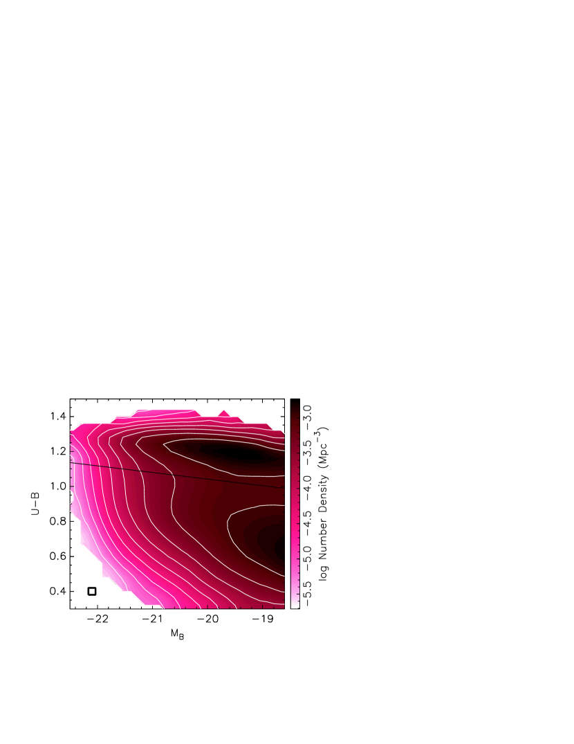
Figure 1: The colour-magnitude diagram of the SDSS galaxies ($0<z<0.2$). The solid line divides the colour bimodality and is defined as $U-B=-0.032*(M_{B}+21.62)+1.175$ (Cooper et al., 2008). The size of a pixel used to smooth the diagram is indicated at bottom left.

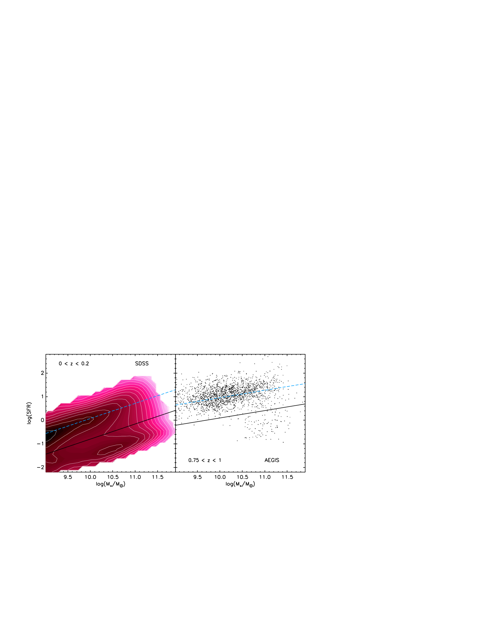
Figure 2: Log SFR vs. log $M_{\rm*}$ for galaxies in two redshift bins. The dashed blue line is a fit to the SF sequence. The solid black line shows the division between the “SF sequence” of galaxies (above the line) and the “low-SFR” or passive galaxies. The text describes how these lines are determined. The weighted ratio of low-SFR galaxies to the total number of galaxies is the “quenched fraction”.

Figure 3: The residuals of the SFR division (solid line in Fig. 2$a$) plotted against the residuals of the rest-frame $U-B$ colour division (solid line in Fig. 1) for the SDSS ($0<z<0.2$). The colour bar on the right shows the number density in a pixel smoothed over adjacent pixels. The size of a pixel is indicated in the bottom left. The galaxies with intermediate SFR lie roughly between the two horizontal dashed lines, with the central horizontal solid line marking the SFR division. The vertical solid line marks the colour division, while the dashed lines roughly delineate the green valley. The SFR bimodality mostly corresponds to the colour bimodality but 30$\%$ of red sequence galaxies lie on the SF sequence while only 4$\%$ of blue cloud galaxies lie below the SF sequence. Also, being in the green valley is not synonymous with transitioning from star formation to quiescence.

3 Bimodality in SFR versus Color

The galaxy bimodality is usually discussed in terms of the bimodality in the colour-magnitude diagram. Fig. 1 shows the colour-magnitude diagram of the SDSS sample with the line dividing the colour bimodality used in Cooper et al. (2008):

$$U-B=-0.032*(M_{B}+21.62)+1.175.$$ (1)

The red sequence, which lies above this line, is assumed to consist mostly of galaxies that have ceased to form stars while the blue cloud (below the line) consists of currently star-forming galaxies. Such a division is convenient because photometry of large samples is easy to do with relatively good accuracy. However, techniques have improved for determining star formation rates for large samples, and we can now divide the galaxies by star formation directly rather than by colour as a proxy.

We show the “physical” version (i.e., reflecting the physical processes of star formation) of the colour-magnitude diagram, namely the SFR-$M_{\rm*}$ diagram for the SDSS and the AEGIS in Fig. 2. The star-forming galaxies lie on a sequence as described by Noeske et al. (2007), which we call the “SF sequence,” while there is a population of galaxies lying under it, which we interchangeably call “low-SFR”, “passive” or “quenched” galaxies. We defined the division between these populations in the following way. We assigned an initial line to divide the population by eye. Then we performed a weighted linear least-squares fit to the points above that line and calculated the distance of each point from the line. After a Gaussian fit to these distances, we then exclude from the SF sequence those points that lie more than $2.5\sigma$ below the line, and re-perform the fit. The process is repeated until no more points are excluded. Quenched galaxies are galaxies that do not lie in the SF sequence as defined in this way. We show the resulting divisions in Fig. 2 with the equation for the dividing line (solid black) being:

$$\log~{}{\rm SFR}=a\log M_{\rm*}-b$$ (2)

where $a$ = [0.64,0.31] and $b$ = [-7.22,-3.04] for the redshift bins [$0<z<0.2$, $0.75<z<1$].

When we refer to ratios of the low-SFR galaxies to the total number of galaxies, we call this the “quenched fraction” rather than the “red fraction” to remind the reader that we divide the galaxies by SFR and not by colour.

In order to compare the SFR bimodality with the colour bimodality, we show in Fig. 3 the residuals from the SFR division $\Delta$ log SFR = log SFR - Eq. (2) versus the residuals from the colour division $\Delta(U-B)=(U-B)-$ Eq. (1) for the SDSS. The horizontal solid line in Fig. 3 corresponds to the solid black line in Fig. 2$a$. As explained above, we call everything above this line a star forming galaxy, or SF sequence galaxy, while everything below it is quenched. Similarly, the vertical solid line in Fig. 3 corresponds to the line in Fig. 1 that divides the red sequence (right of the vertical solid line in Fig. 3) from the blue cloud (left of the vertical solid line). The two horizontal dashed lines are $\pm 0.15$ around the SFR division and are meant to guide the eye to the area of intermediate SFR. The vertical dashed lines are $\pm 0.05$ around the colour division and mark the area of the green valley.

From Fig. 3, we observe that the SFR bimodality mostly corresponds to the colour bimodality, but there are some notable differences. In particular, green valley galaxies are not necessarily intermediate in SFR. Rather about $80\%$ of green valley galaxies are still star forming (lying above the horizonal solid line). Furthermore, about $30\%$ of red sequence galaxies lie in the SF sequence (these are star-forming and are probably reddened by dust - see Brammer et al., 2009 and also Lotz et al., 2008 who find a similar result for $z\sim 1$) whereas only $4\%$ of the blue cloud lie below the SF sequence (these may be post-starburst galaxies, those that exhibit no signs of ongoing star formation but experienced recent star formation within the last $\sim$Gyr - see for example, Dressler & Gunn, 1983; Quintero et al., 2004). Therefore dividing the galaxies by $U-B$ colour does not accurately divide the population by star formation mainly because dusty star formers appear red. We recognise that dust may not explain fully explain the large population of star forming red galaxies since $U-B$ and SFR contain large scatter and are constructed differently. However, these findings are consistent with the results of Maller et al. (2009), who find that about a third of red sequence galaxies in a volume-limited sample of the SDSS at $0.02<z<0.22$ actually lie in the blue cloud after applying an inclination correction to their $M_{g}-M_{r}$ colours, implying a dusty origin to the observed red colours of these galaxies.

These dusty star formers are also the more massive members of the SFR sequence - the dusty star formers are on average 0.4 dex more massive than the entire SF sequence population. This is understandable as the more massive members of the SF sequence are more metal-rich (Tremonti et al., 2004) and therefore have proportionately more dust. This is consistent with the results of Maller et al. (2009) who find that the inclination-dependent colour correction also depends on absolute $K$ magnitude in that brighter galaxies have higher attenuation than dimmer galaxies of the same inclination angle. The fact that massive star-forming galaxies are dusty will cause more massive galaxies to appear quenched if one defines quenching only by colour. This will be important in comparing our results with those of others who define quenching by colour only. We discuss this further in §5.3.

4 Relations between Masses and Environment

In this section, we describe the complex relations between stellar mass $M_{\rm*}$, halo mass $M_{\rm h}$, environment density $\delta_{N}$ and satellite group-centric distance $D$ for central and satellite galaxies in order to prepare the reader for a discussion of quenching as a function of these quantities in the following section. Summarising this section in brief, $M_{\rm h}$ correlates with $M_{\rm*}$ for centrals at low masses, but shows a large spread at high $M_{\rm*}$, offering a chance to separate quenching effects between $M_{\rm*}$ and $M_{\rm h}$ for centrals. $\delta_{N}$ for centrals is a simple two-mode function of $M_{\rm h}$ while for satellites $\delta_{N}$ is given by a complicated interplay between $M_{\rm h}$ and the location within a halo. The dividing line of interpretation of $\delta_{N}$ is where the number of observed group members is less than $N$ (the cross-halo mode) or greater than $N$ (the single-halo mode). Due to the complex nature of $\delta_{N}$, the better measure of local “environment” for satellites may be radial distance from the group centre which is highly anti-correlated with $\delta_{N}$, but only in the single-halo mode. Readers interested mainly in the results of quenching as a function of $M_{\rm*}$, $M_{\rm h}$ and $\delta_{N}$/radial distance may skip to §5.

Note that in all the figures that follow for the SDSS analysis, one quantity is plotted as contours as a function of the $x$- and $y$-axes. These contours are computed in the following way: values of this third quantity are computed in pixels of the indicated size in the plots as long as the pixel contains more than $m$ galaxies (“good” pixels). $m$ is equal to $2\%$ of the average number of galaxies in each pixel which contains at least one galaxy. The values are then smoothed over twice by computing the mean over adjacent good pixels. The pixel sizes are the same in all plots except where noted: 0.2 dex for both the mass quantites ($M_{\rm*}$ and $M_{\rm h}$), 0.3 dex for $\log(1+\delta_{5})$ and 0.15 dex for $\log(d_{\rm prog}/R_{\rm Vir})$. Our pixel sizes and smoothing scheme were chosen to produce acceptably smooth contour lines in order to bring out the main trends. Secondary features should not be taken too seriously.

4.1 $M_{\rm*}$ and $M_{\rm h}$ for centrals

We begin with a discussion of the relation between $M_{\rm*}$ and $M_{\rm h}$. For central galaxies, it has been established with high confidence (e.g., Cacciato et al., 2009; More et al., 2009; Mandelbaum et al., 2009; Leauthaud et al., 2011, 2012) that the relation with the halo mass is somewhat steeper at low mass than at high mass. This is a manifestation of the fact that the halo mass function and the galaxy mass function are considerably different at the low and high mass ends. The result is that $M_{\rm*}$ should correlate closely with $M_{\rm h}$ up to around $M_{\rm crit}$; above this $M_{\rm*}$ begins to level off while $M_{\rm h}$ increases (e.g., Cattaneo et al., 2007, their Figure 2). So $M_{\rm*}$ is a measure of parent $M_{\rm h}$ for $M_{\rm*}$ below a few $\times 10^{10}{\rm M}_{\odot}$, and above that $M_{\rm*}$ serves as a lower limit indicator of $M_{\rm h}$.

In Fig. 4$a$ we show the relation between $M_{\rm*}$ and $M_{\rm h}$ for SDSS central galaxies. Yang et al. (2008) find that galaxies above $M_{\rm h}\sim 10^{12.5}$ follow a very weak scaling of $M_{\rm*}\propto M_{\rm h}^{0.22}$ while below this mass, $M_{\rm*}$ scales more steeply with $M_{\rm h}$, scaling as $M_{\rm*}\propto M_{\rm h}^{1.83}$ for galaxies well below $M_{\rm h}\sim 10^{12.5}{\rm M}_{\odot}$ (Yang et al., 2008). We reproduce this result in Fig. 4$a$ (dashed curve) by fitting their Eq. 7 and obtaining very similar parameters. This flattening of the $M_{\rm*}$-$M_{\rm h}$ relation at high masses reflects the fact that massive centrals occupy groups with a large range of group membership and group masses (since $M_{\rm h}$ corresponds to group $M_{\rm*}$), and presents an excellent opportunity to separate the effects of quenching between $M_{\rm*}$ and $M_{\rm h}$ as we will see in §5.

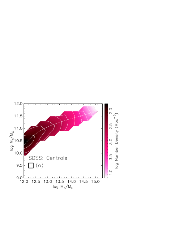
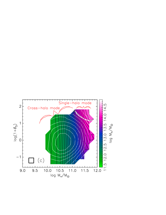
Figure 4: (a). Stellar mass $M_{\rm*}$ versus halo mass $M_{\rm h}$ for SDSS central galaxies ($0<z<0.2$). The dashed curve is a fit to Eq. 7 of Yang et al. (2008). (b) Mean stellar mass $M_{\rm*}$ as a function of density $\log(1+\delta_{5})$ and halo mass $M_{\rm h}$. (c). Mean halo mass $M_{\rm h}$ as a function of density $\log(1+\delta_{5})$ and stellar mass $M_{\rm*}$. The thin white contours in each panel mark the weighted number density of points and are separated by 0.25 dex in density. The thick white lines in (b) and (c) mark where the median membership of a galaxy’s group is six. Membership is greater above this line. The black contours in (b) and (c) follow the coloured shading and are separated by 0.1 dex. The number densities in (a) and the means in (b) and (c) were computed in pixels of the displayed size and smoothed over adjacent pixels. These panels show that: (1) $M_{\rm*}$ correlates with $M_{\rm h}$ for low masses, but massive centrals occupy a large range of halo masses; (2) the single-halo mode is characterised by an increased $\delta_{5}$ and $M_{\rm h}$ while there is no correlation between $\delta_{5}$ and $M_{\rm h}$ in the cross-halo mode; (3) for low $M_{\rm*}$, $M_{\rm h}$ increases with $M_{\rm*}$, and for high $M_{\rm*}$, $M_{\rm h}$ also increases with $\delta_{5}$.

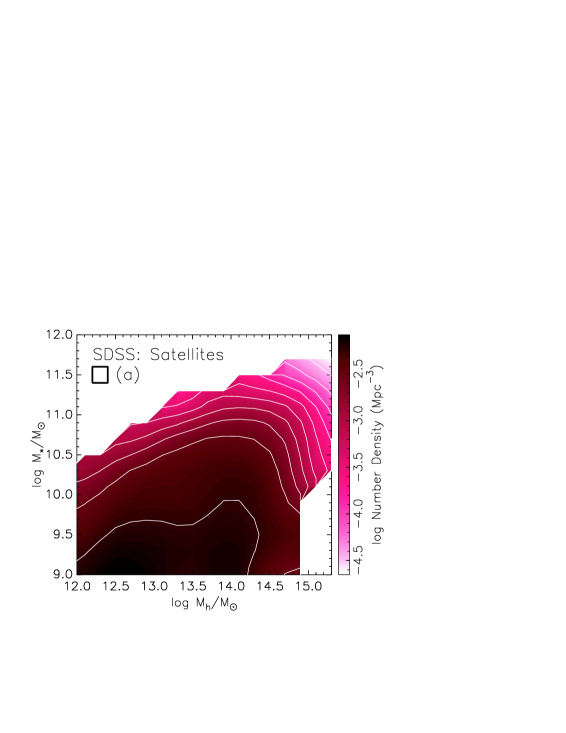
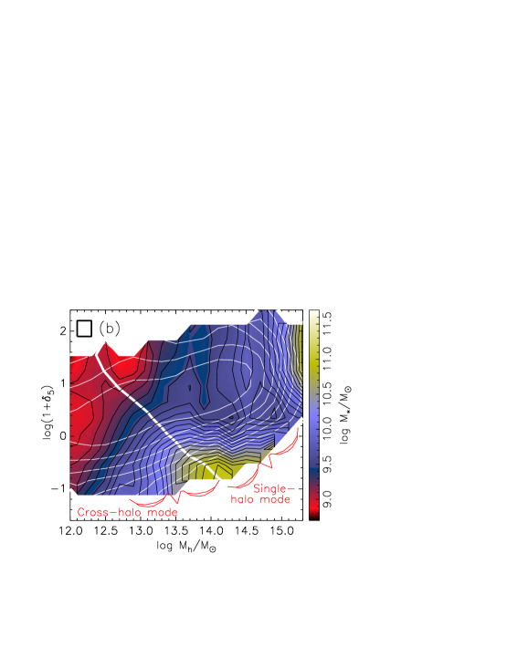
Figure 5: (a). Stellar mass $M_{\rm*}$ versus halo mass $M_{\rm h}$ for SDSS satellites ($0<z<0.2$). (b) Mean stellar mass $M_{\rm*}$ as a function of density $\log(1+\delta_{5})$ and halo mass $M_{\rm h}$. (c). Mean halo mass $M_{\rm h}$ as a function of density $\log(1+\delta_{5})$ and stellar mass $M_{\rm*}$. The thin white contours in each panel mark the weighted number density of points and are separated by 0.25 dex in density. The thick white line in (b) and (c) marks where the median membership of a galaxy’s group is six. Membership is greater above this line. The black contours in (b) and (c) follow the coloured shading and are separated by 0.1 dex. The number densities in (a) and the means in (b) and (c) were computed in pixels of the displayed size and smoothed over adjacent pixels. These panels show that: (1) there is very little correlation between $M_{\rm*}$ and $M_{\rm h}$ for satellites overall; (2) however $M_{\rm*}$ correlates with $M_{\rm h}$ in the cross-halo mode; and (3) in the single-halo mode $\delta_{5}$ correlates with $M_{\rm h}$ as expected in a virialised halo with a halo-occupation function that scales with $M_{\rm h}$.

4.2 $\delta_{N}$ and mass for centrals

As described in §1.1, environment density $\delta_{N}$ for centrals has two modes: the single halo mode measuring field density and the cross-halo mode measuring halo mass. Figs. 4$b$ and $c$ show the distribution of SDSS centrals in the $\delta_{5}$-$M_{\rm h}$ and $\delta_{5}$-$M_{\rm*}$ planes. The thick white curve in the top right corner of panels $b$ and $c$ marks where the median number of group members is six. (More et al., in preparation, give a careful treatment of why lines of constant $N_{\rm members}$ should run more or less parallel to the thick white lines in Figs. 4$b$ and 5$b$.) Above this curve, the centrals are mostly in the single-halo mode of $\delta_{5}$ while below the line, $\delta_{5}$ measures distances to the next halo. The main distribution of centrals in Fig. 4$b$ (marked by the thin white contours) shows very little correlation between $\delta_{5}$ and $M_{\rm h}$ except in the upper right corner where single-halo mode centrals are characterized by the highest $\delta_{5}$ and $M_{\rm h}$. This region of high $M_{\rm h}$, high $\delta_{5}$ corresponds nicely to the increase of $M_{\rm h}$ with $\delta_{5}$ in the upper right corner of Fig. 4$c$ (coloured shading). We also see a deviation from the strong $M_{\rm*}$-$M_{\rm h}$ relation in these region of high $\delta_{5}$. This simply reflects the fact that higher densities in a halo roughly means more satellites, and the summed mass of the satellites will begin to matter, compared to the mass of the central, in the determination of the halo mass.

4.3 $M_{\rm*}$, $M_{\rm h}$ and $\delta_{N}$ for satellites

Fig. 5$a$ shows the $M_{\rm*}$-$M_{\rm h}$ relation for satellites. Unlike for centrals, there is very little correlation between $M_{\rm*}$ and $M_{\rm h}$. For small haloes, $M_{\rm*}$ correlates somewhat with $M_{\rm h}$ in that low-mass haloes do not host massive satellites. But the least massive satellites occupy host haloes of all masses.

Environment density is more complex for satellites than for centrals. More than half (58%) of SDSS satellites reside in groups of six or more members. Fig. 5$b$ and $c$ show the distribution of satellites in the $\delta_{5}$-$M_{\rm h}$ and $\delta_{5}$-$M_{\rm*}$ planes, again with a thick white line marking where the median number of group members is six. Above the line, the satellites reside in groups of more than six members (the single-halo mode).

In the cross-halo mode of $\delta_{N}$, satellites mostly reside in small haloes ($M_{\rm h}\ {\raise-2.15277pt\hbox{$\buildrel<\over{\sim}$}}\ 10^{13}{\rm M}_{\odot}$ - see Fig. 5$b$) with only a few other galaxies. In the cross-halo regions of Fig. 5$b$ and $c$ (under the thick white line), $M_{\rm h}$ roughly correlates with $M_{\rm*}$ (see the coloured shading in these panels). There are at least two reasons why $M_{\rm*}$ for satellites is expected to correlate with $M_{\rm h}$ in this regime. 1) We expect a massive satellite to live in a massive halo, or else it would be the central. Less massive satellites on the other hand are more likely to be merging into a low mass halo, since there are many more of these than massive haloes. 2) The timescale for dynamical friction is inversely proportional to the ratio of the satellite mass to the halo mass (Binney & Tremaine, 1987). So very large satellites relative to the halo will have disappeared into the middle of the halo in a very short time. Therefore, the largest remaining satellite must be some fraction of the halo mass, but smaller than the ratio of the central mass to the halo mass.

In the single-halo mode, $\delta_{N}$ correlates with $M_{\rm h}$ for satellites (see the white density contours of Fig. 5$b$ and the coloured shading of Fig. 5$c$ above the thick white line) just as for centrals again because of the halo profile. Since the halo profile falls off more slowly in a more massive halo, a satellite in a more massive halo will most likely be found near the centre of its halo than if it were in a smaller halo, and its $N$th nearest neighbour would more likely be nearby. For a simpler way to understand the $\delta_{N}$-$M_{\rm h}$ relation for satellites in the single halo mode, assume a uniform distribution of satellites throughout the halo (which is wrong). Recalling that the number of satellites in a halo is $N_{\rm sat}\propto M_{\rm h}^{\alpha}$ where $\alpha$ is close to 1 (see Yang et al., 2008), and recalling that in the spherical collapse model a virialised halo follows $M_{\rm h}\propto R^{3}$, then $1+\delta_{N}\propto N/R^{2}\propto M_{\rm h}^{\alpha-2/3}\sim M_{\rm h}^{1/3}$. Therefore environment density is a measure of the halo mass following something like $\log(1+\delta_{5})\propto\frac{1}{3}\log M_{\rm h}$ which is close to the scaling of the SDSS satellites (Fig. 5$b$).

In the single-halo mode for satellites, we also expect $\delta_{N}$ to be a measure of radial position within a halo. Fig. 6 shows $\delta_{5}$ versus the projected distance $d_{\rm proj}$ of SDSS satellites to their group centres divided by their group virial radii [$R_{\rm vir}=1.2\times 10^{5}(M_{\rm h}/10^{11}{\rm M}_{\odot})^{1/3}{\rm pc}$ (Dekel & Birnboim, 2006)]. As mentioned in §2.1.5, we define $D\equiv d_{\rm proj}/R_{\rm vir}$. In the single-halo mode (above the thick white line which marks where the median group membership is six), higher density indeed means closer proximity to the group centre. In the cross-halo mode, the two quantities do not seem to be related, which is what we expect given that $\delta_{5}$ measures distances to external haloes. (Note that in Fig. 6 the pixel size is smaller than the usual 0.3 dex for $\delta_{5}$ and 0.15 dex for $\log D$ in order to highlight the valley in the contours that separates the single-halo mode from the cross-halo mode.)

A further complication to this already complex nature of $\delta_{N}$ is that whether or not a galaxy is in the single-halo or cross-halo mode of $\delta_{N}$ depends not only on the number of members in its group but also on the limiting magnitude of the survey, which is $z$-dependent. A group of the same mass at $z=0.005$, for example, which appears to be in the single-halo mode will appear to be in the cross-halo mode at $z=0.2$ because some of its members will fall beyond the magnitude limit. In other words, within the SDSS redshift range of $0.005<z<0.2$, the typical distance to the 5th nearest neighbour ranges from 0.34 $h^{-1}$ to 4.0 $h^{-1}$ comoving Mpc (for $0.005<z<0.05$ and $0.15<z<0.2$ respectively). In contrast, $D$ does not behave differently in two modes that depend on the number of fellow group members. (Recall that $R_{\rm vir}$ depends on $M_{\rm h}$ which has been corrected for missing members).

Additionally, although both $\delta_{N}$ and $D$ suffer from projection effects, we expect these effects to be worse for $\delta_{N}$ than for $D$. The Yang et al. (2007) group finder includes or rejects group members based on a $z$-window that is dependent on halo properties (in an iterative way), but $\delta_{N}$ is computed for all galaxies within a fixed $z$-window that is comparable only to the velocity dispersions of the most massive clusters. Since the majority of galaxies are not members of such massive clusters, and since the majority of satellites in the group catalog are not interlopers (Yang et al., 2007), we expect $\delta_{N}$ to suffer from projection more than $D$.

Given these difficulties in interpretating $\delta_{N}$ for satellites, we prefer to use $D$ as a measure of local “environment”. But we have included the popular $\delta_{N}$ variable in our study of quenching in §5 in order to compare with previous work.

For completeness, we replicate Fig. 5$b$ and $c$ in Fig. 7$a$ and $b$, except that we put $D$ on the $y$-axis instead of $\log(1+\delta_{5})$. In panel $a$, we see that the dual-modes of $\delta$ that we saw in Fig. 5$b$ disappear as expected. For example, the two regions of high $M_{\rm*}$ in Fig. 5$b$ become one region in Fig. 7$a$.

In Fig. 7$b$, the dynamical range of $M_{\rm h}$ diminishes compared to Fig. 5$c$. This is because low-mass haloes will never host very many satellites (nor very massive satellites) and $\delta_{5}$ for these satellites will almost always be in the cross-halo mode; 90% of satellites in haloes of masses $10^{12-12.7}{\rm M}_{\odot}$ live in haloes with fewer than six members, so their $\delta_{5}$ is forced to be low. This is why the lower left corner of Fig. 5$c$ is coloured deep green (low $M_{\rm h}$). But these same satellites have no such restriction on $D$. Some of them could reside very near their group centres even if their $\delta_{5}$ is low. Furthermore, if their masses are low, they could reside in haloes of all masses. For these two reasons, there are no regions in Fig. 7$b$ with very low average $M_{\rm h}$.

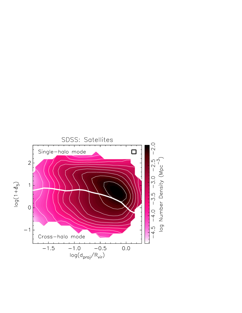
Figure 6: The environment density of SDSS satellites ($0<z<0.2$) versus their projected distance to their group centres relative to their virial radii ($d_{\rm proj}/R_{\rm vir}$) . The thick white line marks the dividing line between groups with six or more members (above the line) and fewer than six members (below the line). Single-halo mode is above this line, cross-halo mode is below. Note how the valley in the contour lines tends to follow this line. In the single-halo mode, proximity to the group centre is clearly associated with an increase in $\delta_{5}$, while in cross-halo mode, there is no relationship. This is expected based on the statistics of these relationships.

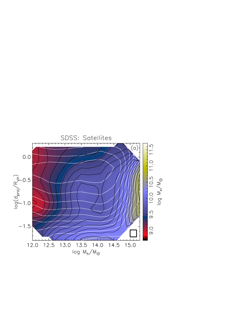
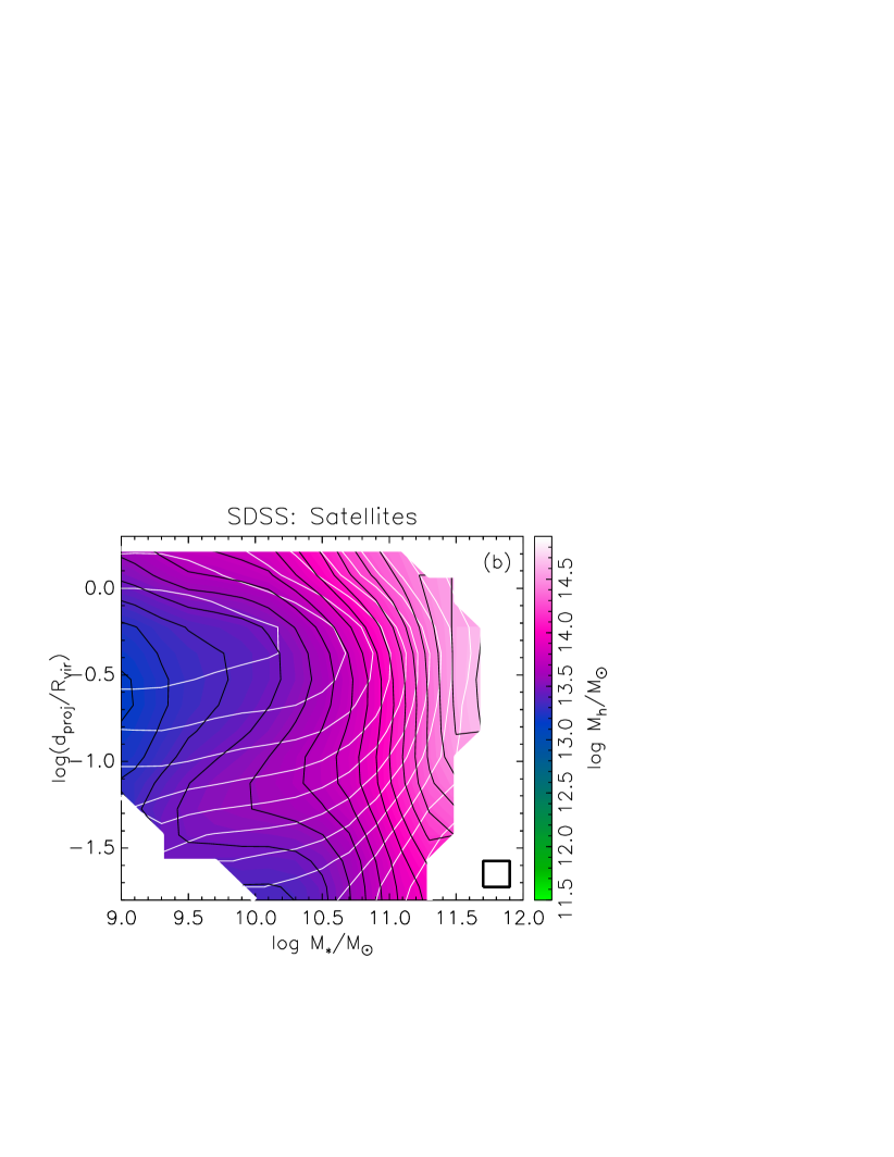
Figure 7: (a) Mean stellar mass $M_{\rm*}$ as a function of relative group distance $D=d_{\rm proj}/R_{\rm vir}$ and halo mass $M_{\rm h}$. (b). Mean halo mass $M_{\rm h}$ as a function of relative group distance $D$ and stellar mass $M_{\rm*}$. The thin white contours in each panel mark the weighted number density of points and are separated by 0.25 dex in density. The black contours in follow the coloured shading and are separated by 0.1 dex. The means were computed in pixels of the displayed size and smoothed over adjacent pixels. These panels show that: (1) the $D$-$M_{\rm h}$ plane does not exhibit dual-mode behaviour as in Fig. 5$b$; (2) the dynamical range of mean $M_{\rm h}$ in the $D$-$M_{\rm*}$ plane is diminished compared to the $\delta_{5}$-$M_{\rm*}$ plane.

5 Main Results: Quenching and Halo Environment

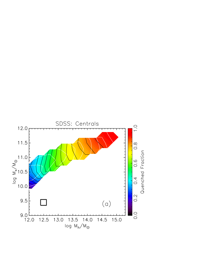
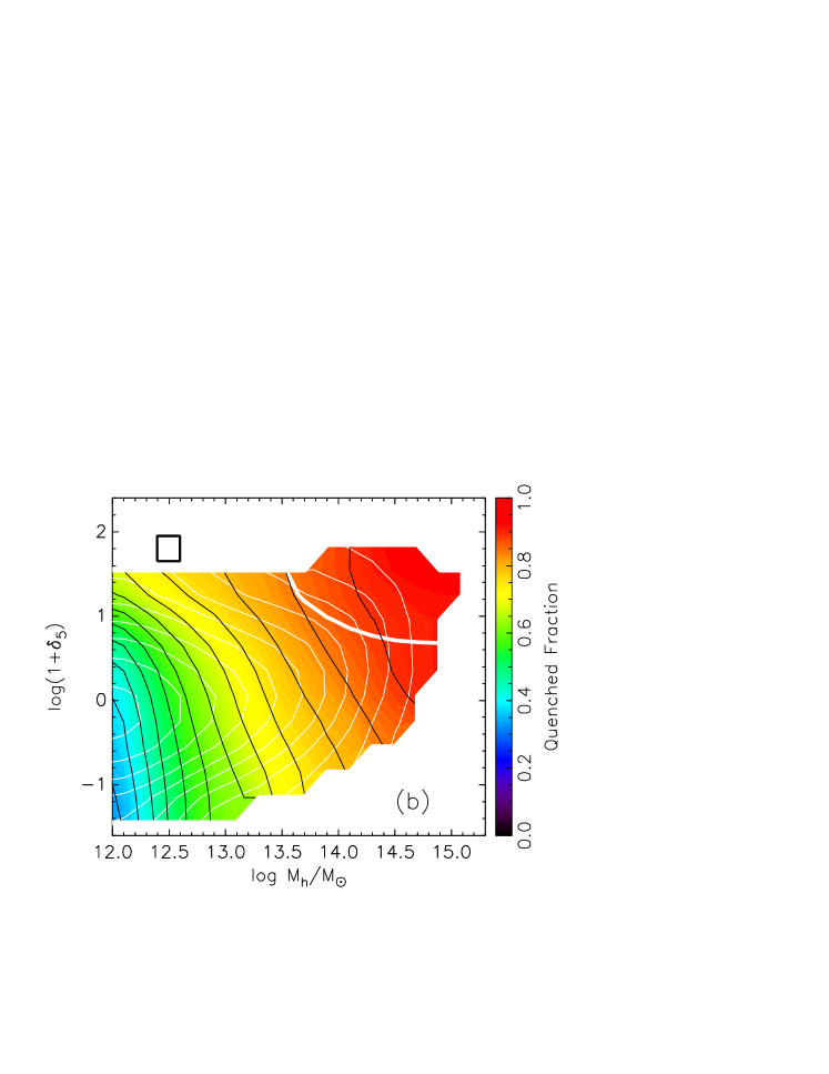
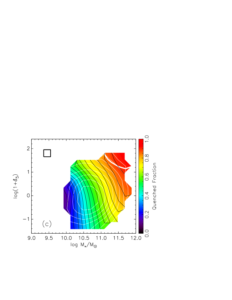
Figure 8: The mean quenched fraction as a function of $M_{\rm*}$ and $M_{\rm h}$ (a), of $\delta_{5}$ and $M_{\rm h}$ (b), and of $\delta_{5}$ and $M_{\rm*}$ (c) for central galaxies in the SDSS ($0<z<0.2$). The thin white contours in each panel mark the weighted number density of points and are separated by 0.25 dex in density. The thick white line marks where the median membership of a galaxy’s group is six. Membership is greater above this line. The black contours follow the coloured shading and are separated by 0.05. The means were computed in pixels of the displayed size and smoothed over adjacent pixels. To first approximation, the quenched fraction for centrals correlates with $M_{\rm h}$ more strongly than with $M_{\rm*}$ or $\delta_{5}$ as shown by the vertical black contours in panel $a$ and $b$. Quenching in $c$ roughly follows mean $M_{\rm h}$ (see Fig. 4$c$).

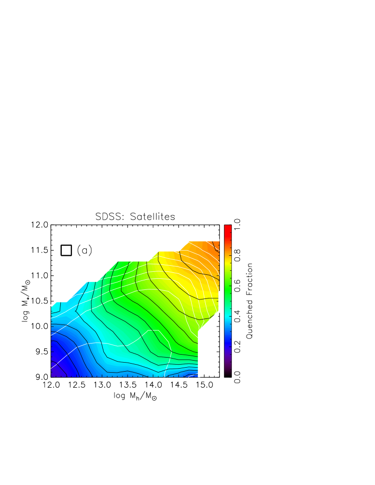
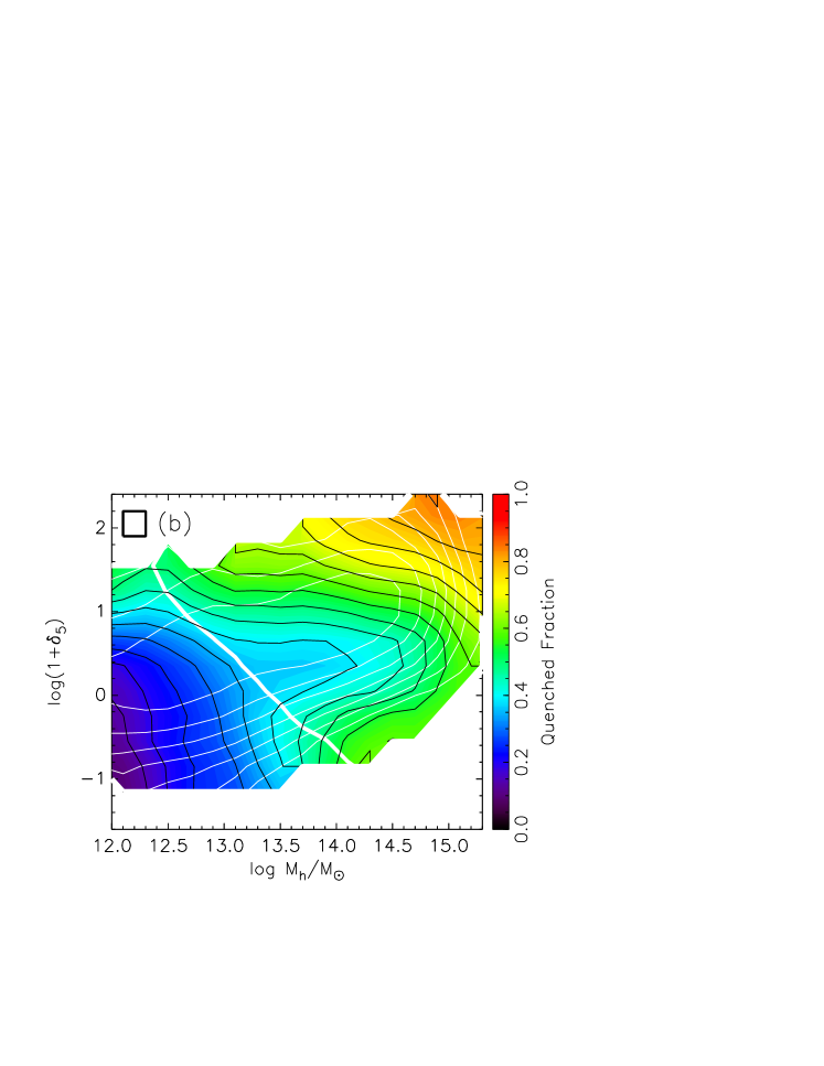
Figure 9: The mean quenched fraction as a function of $M_{\rm*}$ and $M_{\rm h}$ (a), of $\delta_{5}$ and $M_{\rm h}$ (b), and of $\delta_{5}$ and $M_{\rm*}$ (c) for satellite galaxies in the SDSS ($0<z<0.2$). The thin white contours mark the weighted number density of points and are separated by 0.25 dex in density. The thick white line marks where the median membership of a galaxy’s group is six. Membership is greater above the thick line. The black contours follow the coloured shading and are separated by 0.05. The means were computed in pixels of the displayed size and smoothed over adjacent pixels. Quenching for satellites correlates with all three quantities $M_{\rm h}$, $M_{\rm*}$ and $\delta_{5}$. None of these panels contains regions of very high mean quenched fraction, indicating that, in contrast to centrals, the combination of $M_{\rm*}$, $M_{\rm h}$ and $\delta_{5}$ is not optimum for expressing the quenched fraction of satellites.

In the previous section we explored the relations between stellar mass, halo mass and environment density for satellite and central galaxies in the SDSS. We showed that for central galaxies, $M_{\rm*}$ correlates with $M_{\rm h}$ for low masses, but massive centrals of a given stellar mass occupy a large variety of halo masses. We also showed that the single-halo mode of $\delta_{5}$ for centrals is characterised by increasing $M_{\rm h}$ with increasing $\delta_{5}$ while in the cross-halo mode, there is little correlation between $\delta_{5}$ and $M_{\rm h}$. For satellite galaxies, there is a weak correlation between $M_{\rm*}$ and $M_{\rm h}$ in the cross-halo mode only. In the single-halo mode, $\delta_{5}$ for satellites correlates with $M_{\rm h}$ as expected for virialised haloes with a halo-occupation function that scales with $M_{\rm h}$. Since we now know how these quantities relate to each other, we are in a position to explore quenching as a function of these quantities.

5.1 Quenching for centrals

Fig. 8 repeats the panels of Fig. 4 ($M_{\rm*}$ and $M_{\rm h}$, $\delta_{5}$ and $M_{\rm h}$, and $\delta_{5}$ and $M_{\rm*}$) but now shows the fraction of quenched galaxies as the third parameter represented by the colour gradient. Fig. 8$a$ is the key result of this paper. It shows that the quenched fraction appears to increase more strongly with $M_{\rm h}$ at fixed $M_{\rm*}$ than with $M_{\rm*}$ at fixed $M_{\rm h}$ for central galaxies. The contour lines of the quenching to first order follow $M_{\rm h}$, not $M_{\rm*}$, i.e., they are roughly vertical above $M_{\rm*}\sim 10^{10.4}{\rm M}_{\odot}$. The quenched fraction increases by less than $\sim 0.1$ over 0.8 dex, or 40% of the range in $M_{\rm*}$ (at constant $M_{\rm h}$), but increases by almost 0.35 over 40% of the $M_{\rm h}$ range (at constant $M_{\rm*}$). This result seems to prefer halo-quenching models over mechanisms that are more closely tied to $M_{\rm*}$ such as the QSO mode of AGN feedback. Note that the halo environment heated by a virial shock is more likely to host the radio mode of AGN (Dekel & Birnboim, 2006) because the coupling of the AGN energy to the halo gas is more efficient when the gas is hot.

To second order, Fig. 8$a$ shows a small dependence of quenching on $M_{\rm*}$ at constant $M_{\rm h}$ for massive haloes. This can be explained in the following way. After a virial shock forms in a massive halo, residual cold gas may still form stars inside the galaxy after the shock has been triggered. An $M_{\rm*}$ dependence could then naturally arise if at fixed $M_{\rm h}$, a central with higher stellar mass had converted more of any residual gas into stars, exhausting its gas supply, and making it more susceptible to quenching. However, this $M_{\rm*}$-dependence of the quenching seems to be a secondary effect compared to the dominant trend of quenching with $M_{\rm h}$ as seen in Fig. 8$a$.

Fig. 8$b$ shows quenching in the $\delta_{5}$-$M_{\rm h}$ plane. It reveals that the quenched fraction increases with $M_{\rm h}$ and only weakly with $\delta_{5}$. At constant $M_{\rm h}$, the quenched fraction increases at the most by 0.2, and for most masses only by 0.1, over two orders of magnitude in $\delta_{5}$. However at constant $\delta_{5}$, the quenched fraction increases by as much as 0.4 over two orders of magnitude in $M_{\rm h}$.

When we examine quenching in the $\delta_{5}$-$M_{\rm*}$ plane (Fig. 8$c$), especially at large $\delta_{5}$, we see that the quenched fraction for centrals depends on both $\delta_{5}$ and $M_{\rm*}$. The increase of the quenched fraction with $M_{\rm*}$ is consistent with the increase of $M_{\rm h}$ with $M_{\rm*}$ below $M_{\rm*}\sim 10^{11}{\rm M}_{\odot}$ (see Fig. 4$c$). Above this mass, the quenched fraction increases with $\delta_{5}$ in a way similar to the increase of $M_{\rm h}$ with $\delta_{5}$ in Fig. 4$c$. Thus, apart from the low $M_{\rm*}$ and high $\delta_{5}$ region, the quenching pattern in Fig. 8$c$ is explainable by a basic trend of quenched fraction with $M_{\rm h}$. In §4 we discussed that the $M_{\rm h}$ pattern in Fig. 4$c$ is the result of the interplay between the two modes of $\delta_{N}$ and the weakening of the $M_{\rm*}$-$M_{\rm h}$ relation for massive centrals. Thus the quenching pattern in the $\delta_{5}-M_{\rm*}$ plane is consistent with a correlation of quenching with $M_{\rm h}$. Note that Peng et al. (2011) did not find the $\delta_{5}$ dependence of the quenched fraction at high $M_{\rm*}$ mostly because they defined quenching by colour and not by SFR - more on this in §5.3.

The dependence of quenching on $\delta_{5}$ at low to intermediate $M_{\rm h}$ and at high $\delta_{5}$ (see Fig. 8$b$, also reflected in $c$ at low $M_{\rm*}$) is not a neccessary trend in the simple theoretical framework of halo quenching that we have been advancing. This may possibly be attributed to misclassified satellites (an explanation suggested by Peng et al., 2011). However, we can offer another explanation that takes the classification at face value and appeals to the halo quenching mechanism. Halo masses on the order of $M_{\rm crit}$ may be capable of sustaining a stable virial shock without actually containing one. It has been seen in cosmological simulations that, once the halo mass is $\sim M_{\rm crit}$, the trigger for the formation of a shock that quickly expands to the virial radius is typically an occasional minor merger. Small centrals that have a high $\delta_{N}$ must have one or more external haloes nearby, and are therefore more likely to capture loose satellites of these neighbouring haloes, which may trigger the virial shock that causes quenching. This explanation predicts a higher quenched fraction at the highest values of $\delta_{5}$ in halo somewhat below $M_{\rm crit}$, as is observed.

An astute reader may notice that the quenched fraction seems to reach lower levels when using $M_{\rm*}$ (Fig. 8$c$) than when using $M_{\rm h}$ (Fig. 8$b$). These lower levels of quenching at low $M_{\rm*}$ compared to low $M_{\rm h}$ reflect the fact that the quenching contours in Fig. 8$a$ are close to horizontal for $M_{\rm*}\ {\raise-2.15277pt\hbox{$\buildrel<\over{\sim}$}}\ 10^{10.4}{\rm M}_{\odot}$ and $M_{\rm h}\ {\raise-2.15277pt\hbox{$\buildrel<\over{\sim}$}}\ 10^{12.5}{\rm M}_{\odot}$. This is the regime where $M_{\rm h}$-dependent quenching is not expected to be important (since $M_{\rm h}$ is below or around $M_{\rm crit}$). It is here that residual $M_{\rm*}$-dependent quenching becomes important, and this regime will be explored further in §6.1.

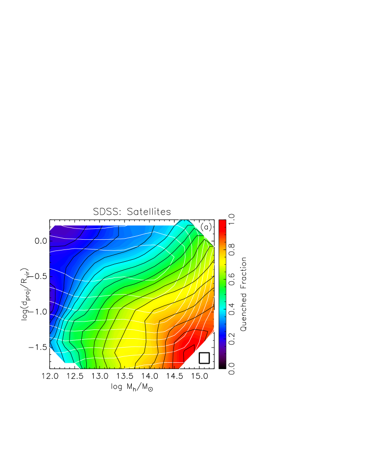
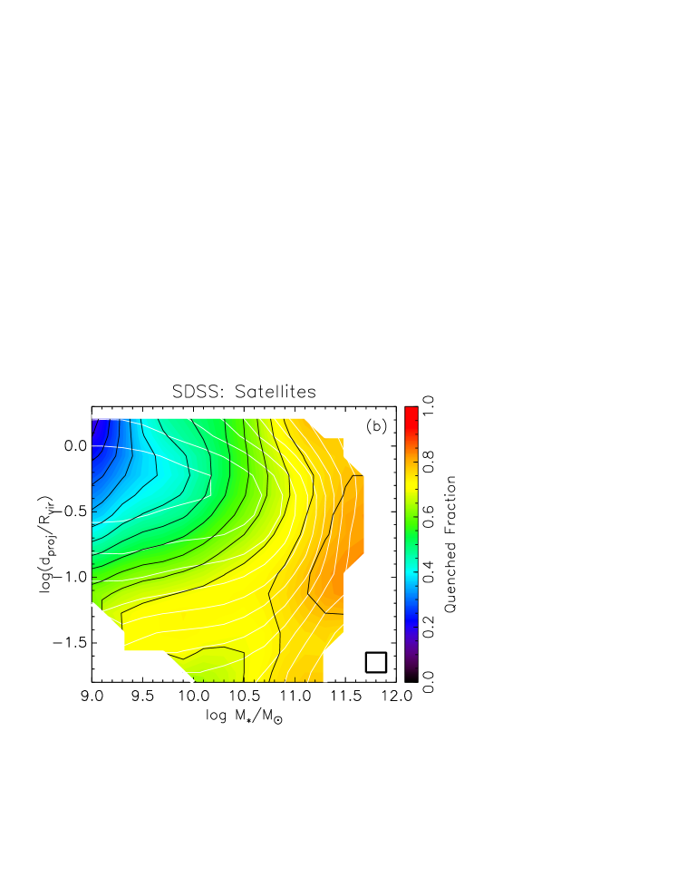
Figure 10: The mean quenched fraction of SDSS satellites ($0<z<0.2$) as a function of the projected distance to the group centre relative to the group virial radius ($d_{\rm proj}/R_{vir}$) and the halo mass $M_{\rm h}$ (a) and stellar mass (b). The thin white contours in each panel mark the weighted number density of points and are separated by 0.25 dex in density. The black contours follow the coloured shading and are separated by 0.05. The means were computed in pixels of the displayed size and smoothed over adjacent pixels. Quenching for satellites increases with $M_{\rm h}$ and decreases with $D=d_{\rm proj}/R_{\rm vir}$. Quenching also increases with $M_{\rm*}$ at large $D$ where $M_{\rm h}$-quenching is weakest and where the satellites likely fell in recently, suggesting a quenching dependence on the sub-halo. Satellites closer to the group centre than $\sim 0.2R_{\rm vir}$ likely fell in less recently, and their quenched fraction depends strongly on host $M_{\rm h}$ and almost not at all on satellite $M_{\rm*}$.

A correlation between the quenched fraction and halo mass at fixed stellar mass, for centrals, is expected on theoretical grounds based on the critical mass for virial shock heating, as in Birnboim & Dekel (2003), Kereš et al. (2005), and Dekel & Birnboim (2006). We note, however, that a detected correlation does not necessarily imply causation, and that one should apply caution because the halo mass and the stellar mass are not independent of each other. Indeed, at low masses, $M_{*}<10^{11}{\rm M}_{\odot}$ and $M_{h}<10^{12}{\rm M}_{\odot}$, halo mass and stellar mass are expected to grow in concert, while at larger masses the stellar mass tends to a constant as the halo mass keeps growing (e.g., Cooray & Milosavljević, 2005; Yang et al., 2012). Can this introduce an apparent correlation of the quenched fraction with $M_{h}$ at a fixed $M_{*}$ in an alternative scenario where the ”true” cause of quenching is associated with $M_{*}$ and not with $M_{h}$? It can clearly introduce a general trend, where the average halo mass of quenched galaxies is larger than for un-quenched galaxies, but it is not expected to introduce a continuous gradient of the quenched fraction with $M_{h}$ at a given $M_{*}$ all the way to $10^{15}{\rm M}_{\odot}$, and no correlation of the quenched fraction with $M_{*}$ at a given $M_{h}$, as in Fig. 8$a$. We conclude from Fig. 8$a$ that the direct contribution of halo mass to quenching seems to be more fundamental than the contribution of stellar mass.

5.2 Quenching for satellites

Fig. 9 shows the equivalent of Fig. 8, but for satellites. In all three panels of Fig. 9, the quenched fraction for satellites increases with all three quantities $M_{\rm h}$, $M_{\rm*}$ and $\delta_{5}$ suggesting that these three projections are not the most helpful way to understanding the main drivers of quenching for satellites. As argued in §4, $\delta_{N}$ for satellites is a complicated quantity, whose properties change according to the choice of $N$, on limiting magnitudes. Furthermore, $M_{\rm*}$ for satellites is expected to correlate with their position in their host halo, e.g., because dynamical friction causes massive satellites to spiral inward faster than less massive ones. Moreover, less massive satellites suffer from colour-dependent incompleteness. A mass-limited cut on the satellite sample which would make it complete for red galaxies (following the cut applied by Dutton et al., 2011: $M_{\rm*}>10.7+\log(z/0.1)$) includes very few galaxies smaller than $M_{\rm*}\sim 10^{10.3}{\rm M}_{\odot}$ and excludes more than half the satellite sample.

In light of these difficulties in interpreting Fig. 9, we complement Figs. 9$b$ and $c$ with Figs. 10$a$ and $b$, replacing $\delta_{5}$ on the $y$-axis with the simpler projected radial distance from the centre ($D\equiv d_{\rm proj}/R_{\rm vir}$). (Recall from Fig. 6 that $\delta_{N}$ correlates with $D$ in the single-halo mode of $\delta_{N}$.)

Fig. 10$a$ shows that the quenched fraction for satellites increases with both halo mass and with proximity to the group centre. The quenching trend with radial distance is strongest for distances of greater than $\sim$0.1-0.2$R_{\rm vir}$. Below this, the motions of satellites and/or projection effects may smear out the quenching trend with $D$, causing quenching to appear to increase only with $M_{\rm h}$. However we do not expect projection effects to be strong, especially in massive haloes which contain many satellites at small radial distance so the signal-to-noise for small $D$ is higher.

Fig. 10$b$ shows that the quenched fraction also increases with satellite stellar mass $M_{\rm*}$ for constant $D$. The $M_{\rm*}$ dependence is strongest for satellites at the farthest distances from the centre, where the $M_{\rm h}$ dependence is weakest (but even here, the $M_{\rm h}$-dependence of the quenched fraction is not that weak, increasing by more than 0.3 over 2.5 dex). If we assume that these galaxies at large $D$ have only just fallen into a larger halo, their quenching dependence on $M_{\rm*}$ is consistent with a quenching dependence on the mass of their own halo before infall, now sub-halo, since $M_{\rm h}$-dependent quenching operated on them while they were still centrals (Fig. 8$a$). The $M_{\rm*}$ dependence in Fig. 10$b$ virtually disappears for satellites closer to the centre than $\sim 0.2R_{\rm vir}$, where the $M_{\rm h}$ dependence is the strongest. If these satellites have resided in their host haloes for some time, the quenching processes which operate in the host halo and which depend on the host $M_{\rm h}$ will eventually affect the satellites so that their quenched fraction will depend strongly on host $M_{\rm h}$ rather than on the satellite $M_{\rm*}$ as we see in Fig. 10.

Fig. 10$a$ succeeds in identifying the properties of satellites that produce high quenched fractions of $\ {\raise-2.15277pt\hbox{$\buildrel>\over{\sim}$}}\ 0.95$, namely high $M_{\rm h}$ and close proximity to the halo centre. None of the panels in Fig. 9 or Fig. 10$b$ produce regions of the plot with such high quenched fraction. This seems to suggest that it is a combination of halo mass and distance to the halo centre that governs quenching in satellites.

In terms of dynamical range of quenching, however, the combination of $D$ and $M_{\rm h}$ produces a range as broad as the pair $\delta_{5}$ and $M_{\rm h}$ (Fig. 9$b$) or even the pair $\delta_{5}$ and $M_{\rm*}$ (Fig. 9$c$). However, quenching trends with $\delta_{5}$ are difficult to interpret due to the dual nature of $\delta$. Which mode of $\delta$ a satellite belongs to depends on redshift as discussed earlier, in that a galaxy in the single-halo mode at low $z$ will appear to be in the cross-halo mode at high $z$ because some members of its group will drop out of the magnitude limit. Furthermore, these satellites with spuriously low $\delta_{5}$ will likely be bluer on average than the true population, especially at lower mass, since low mass red galaxies are selected against at higher $z$. Indeed, when we checked the sub-sample with $z<0.05$, satellites with $-1<\delta_{5}<0$ and $9<\log M_{\rm*}/{\rm M}_{\odot}<10.5$ had quenched fractions 0.1 higher than the whole redshift sample in these $\delta_{5}$ and $M_{\rm*}$ ranges, whereas the quenched fraction in the $D$-$M_{\rm h}$ plane did not change. For these reasons, quenching trends with $\delta_{5}$ may be somewhat exaggerated, and $D$ is the preferred predictor of quenching.

As for whether $M_{\rm h}$ or $M_{\rm*}$ is better at predicting quenching for satellites, Fig. 9$a$ seems to indicate that they are equally good. However, quenching seems to follow average $M_{\rm h}$ better than average $M_{\rm*}$. Specifically, the quenching contours in Fig. 9$c$ roughly follow the $M_{\rm h}$ contours in Fig. 5$c$, while the quenching contours in Fig. 9$b$ do not follow the $M_{\rm*}$ contours of Fig. 5$b$. Similarly, the quenching contours in Fig. 10$a$ do not follow the $M_{\rm*}$ contours in Fig. 7$a$ (except at high $D$) while the quenching contours in Fig. 10$b$ do somewhat follow the $M_{\rm h}$ contours in Fig. 7$b$ (except at high $D$). (Quenching at the high $D$ as we argued above may be following sub-halo mass more than host halo mass.)

In summary, we have found that the combination of halo mass and distance to the halo centre is an excellent predictor of quenching for satellites, producing high quenched fractions of $\ {\raise-2.15277pt\hbox{$\buildrel>\over{\sim}$}}\ 0.95$. Combinations involving $\delta_{5}$ and $M_{\rm*}$ also produce large dynamic range of quenching, but this may be due to a lucky combination of redshift effects and sub-halo effects.

The trend of the quenched fraction with radial distance from the group centre is consistent with external mechanisms of quenching such as the halo quenching model, where virial shock heating is most efficient for large halo masses and in the centres of haloes. In such a scenario, quenching is expected to be a function of the density of the hot gas which increases with decreasing radial distance to the centre as well as with $M_{\rm h}$. This trend of quenching with proximity to the centre is also consistent with other processes such as strangulation, tidal stripping and ram pressure stripping.

5.3 Comparisons with previous work

Our finding that quenching increases primarily with $M_{\rm h}$ rather than $M_{\rm*}$, and is also correlated with $D$ for satellites, is consistent with the findings of Weinmann et al. (2006a) who find that halo mass is more important than luminosity in predicting galaxy properties (and improves on their result as $M_{\rm*}$ is a more intrinsic internal property than $L$).

Our study improves on that of Kimm et al. (2009) who show similar plots as Fig. 8$a$ and Fig. 9$a$ and could not decide which of $M_{\rm*}$ and $M_{\rm h}$ was more important for quenching in centrals. For satellites they argued that $M_{\rm*}$ and $M_{\rm h}$ were equally important for quenching. We have improved on their analysis by combining $M_{\rm*}$- and $\delta_{5}$-dependent quenching into a dependence on $D$ and $M_{\rm h}$. For centrals, we have improved on their result by smoothing the quenched fraction over the $M_{\rm*}$-$M_{\rm h}$ plane in order to discern the overall trend of quenching with $M_{\rm h}$. The slight $M_{\rm*}$-dependence of the quenched fraction for centrals with high $M_{\rm h}$ is similar to that found in Kimm et al. (2009), but we have shown that the the overall quenching trend with $M_{\rm h}$ is stronger.

Note also that Kimm et al. (2009) use stellar masses that were computed using the models of Bell et al. (2003) which can underestimate $M_{\rm*}$ for dusty, star-forming galaxies (for a typical dust model with attenuations of 1.6 and 1.3 in the $g$ and $r$ bands, $M_{\rm*}$ will be underestimated by 0.2 dex: see Bell et al., 2003). Underestimating $M_{\rm*}$ for star forming galaxies but not for quiescent galaxies has the effect of exaggerating quenching trends with $M_{\rm*}$ at fixed $M_{\rm h}$. In contrast, the values of $M_{\rm*}$ that we use are estimated by SED fitting taking dust into account (see the references in §2.1.4).

One may worry that the group stellar masses of Yang et al. (2007), computed using Bell et al. (2003), also result in exaggerated quenching trends with $M_{\rm h}$. However, we do not expect this effect to be large especially above $M_{\rm h}\sim 10^{13}{\rm M}_{\odot}$ where the centrals are more than 70% quenched and their masses contribute less than 75% of their group mass. To test the effect of dust on the $M_{\rm h}$ estimates, we performed a rough rescaling of the Yang et al. $M_{\rm h}$ values to reflect group masses based on Brichmann et al. $M_{\rm*}$ estimates, and find that the quenched fraction increases more than twice as much with $M_{\rm h}$ at fixed $M_{\rm*}$ than with $M_{\rm*}$ at fixed $M_{\rm h}$ over the same range of mass. This is despite the uncertainties in $M_{\rm h}$ being much larger ($>0.3$ dex) than the typical uncertainties in $M_{\rm*}$ ($<0.05$ dex). So, after considering dust, our result that $M_{\rm h}$ predicts quenching more than $M_{\rm*}$ appears to be robust. (More on dust below.)

Our result that quenching of satellites correlates with $M_{\rm h}$ and anticorrelates with $D$ is consistent with the results of Blanton & Berlind (2007) and Hansen et al. (2009) (who use group luminosity and group richness rather than $M_{\rm h}$). The decreased quenching with $D$ also agrees with several other studies of SFR or the blue/red fractions within groups and clusters (Gómez et al., 2003; Balogh et al., 2004; Tanaka et al., 2004; Rines et al., 2005; Haines et al., 2007; Wolf et al., 2009; von der Linden et al., 2010). (See also Diaferio et al., 2000; Springel et al., 2001; Weinmann et al., 2010 for semi-analytic model recipes that reproduce these trends).

Our results also agree with those of Wetzel et al. (2012a) who find that quenching for satellites correlates with $M_{\rm h}$ and $D$ at fixed $M_{\rm*}$. Wetzel et al. (2012b) also demonstrated that the distribution of specific SFR for satellites can be explained by considering the satellites’ time since first infall. De Lucia et al. (2012) also showed using a semi-analytic cosmological model that satellite distance from the group/cluster centre is correlated with the time of accretion. This is consistent with our finding that the satellite quenched fraction increases with $M_{\rm*}$ at higher $D$ values. Since these satellites recently fell in, their quenched fraction reflects their sub-halo mass rather than their host halo mass. But some time after the first infall (2-4 Gyr: Wetzel et al., 2012a; 5-7 Gyr: De Lucia et al., 2012), halo quenching takes over so that quenching for satellites closer than $\sim 0.2R_{\rm vir}$ depends strongly on their host halo mass.

While Bamford et al. (2009) found that the red fraction of galaxies increases with $M_{\rm*}$ and environment (as measured by $\delta_{N}$ and the distance to the nearest galaxy group), they also found that the red fraction does not vary strongly with group mass (see their Fig. 13). This at first sight seems to contradict our result that quenching depends on $M_{\rm h}$ (derived from group mass). However, these authors use the C4 Cluster Catalog of Miller et al. (2005) which does not include isolated galaxies. The membership of each group ranges from 10 to more than 200 galaxies so that Fig. 13 of Bamford et al. (2009) is dominated by satellites. As we showed in Fig. 10$a$, both $M_{\rm h}$ and $D$ are needed to predict quenching for satellites. Most satellites lie at 0.3-1$R_{\rm vir}$ from their group centres (white contours of Fig. 10$a$) which is where the $M_{\rm h}$-dependence of quenching is weakest. Therefore, measuring the quenched fraction of satellites as a function of $M_{\rm h}$, regardless of $D$, will result in a weak $M_{\rm h}$ dependence of quenching. This also seems to be the main reason why van den Bosch et al. (2008) find only weak correlation between satellite colour and $M_{\rm h}$ and between satellite colour and $D$.

Our analysis improves on the interpretation of Peng et al. (2010, 2011) who find that mass determines quenching for both centrals and satellites, while $\delta_{5}$ also governs quenching for satellites. They do not distinguish between stellar mass and halo mass for centrals (for satellites, see below). While quenching for centrals apparently depends on $M_{\rm*}$ (Fig. 8$c$), we have found that quenching correlates more strongly with $M_{\rm h}$ at fixed $M_{\rm*}$ than with $M_{\rm*}$ at fixed $M_{\rm h}$ (Fig. 8$a$). We also related the $\delta_{5}$ and $M_{\rm*}$ dependence of quenching for satellites to a quenching relation with $D$ and $M_{\rm h}$ and argued that these are the preferred predictors of quenched fraction.

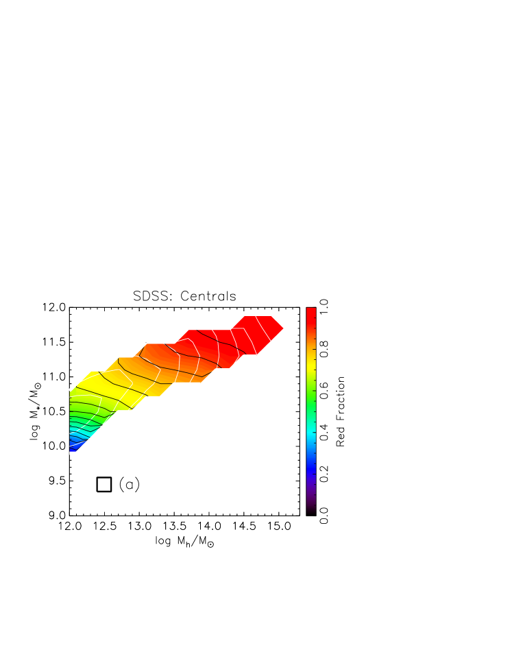
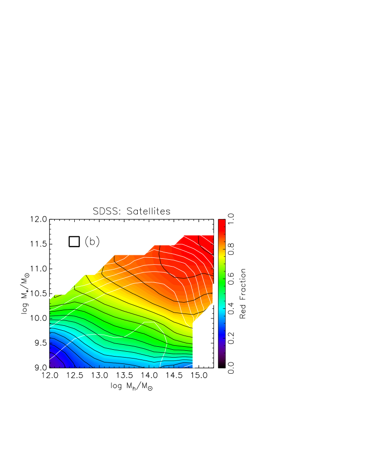
Figure 11: The mean red fraction as a function of $M_{\rm*}$ and $M_{\rm h}$ for centrals (a) and satellites (b) in the SDSS ($0<z<0.2$). The thin white contours in each panel mark the weighted number density of points and are separated by 0.25 dex in density. The black contours follow the coloured shading and are separated by 0.05. The means were computed in pixels of the displayed size and smoothed over adjacent pixels. To first approximation, the red fraction for centrals correlates with $M_{\rm*}$ more strongly than with $M_{\rm h}$ for both centrals and satellites. The red fraction behaves differently from the quenched fraction (Fig. 8$a$, 9$a$) because red galaxies which are still forming stars are on average more massive than the star-forming population.

However, Peng et al. (2011) find that for satellites, $M_{\rm*}$-quenching is more important than $M_{\rm h}$-quenching at a fixed $\delta_{5}$, namely for $1.0<\log(1+\delta_{5})<1.3$. But this is not the whole quenching picture. Using Fig. 6, this narrow range of $\delta_{5}$ corresponds to a $\log D$ of about -0.4 which is in the region of Fig. 10 where satellites only recently fell in. Here, quenching relates to the sub-halo and the host halo mass will not matter much. But we demonstrated that quenching of satellites strongly increases with $M_{\rm h}$ (and almost not at all with $M_{\rm*}$) for satellites closer to the group centre than $\sim 0.2R_{\rm vir}$ where we expect the time since infall to be long.

5.4 SFR vs. Colour

Lastly, we caution that measuring quenching by colour rather than by SFR causes $M_{\rm*}$-dependent quenching to appear stronger and $M_{\rm h}$-dependent quenching to appear weaker than they actually are. The reason is that colour as a quenching proxy is severely contaminated by dust. As described in §3, one third of the red sequence galaxies are in fact not quenched but are dusty star-formers. These predominantly lie on the massive end of the SF sequence (but share a similar mass distribution to that of the red sequence). Thus, dividing the galaxies by colour removes many of the massive galaxies from the “star forming” sample, leaving an overall less massive “blue” sample (by about 0.4 dex). (This same exercise does not render the “red” sample with a significantly different mass distribution as the “passive” sample). Therefore, the red fraction will appear to correlate with $M_{\rm*}$ more than the quenched fraction. Furthermore, since $M_{\rm*}$ and $M_{\rm h}$ do not correlate for satellites, and only very weakly for centrals at the massive end, the red fraction will appear to correlate more with $M_{\rm*}$ than with $M_{\rm h}$. And this is the reason why Peng et al. (2011) missed the significant $\delta_{5}$-dependent quenching for centrals at the massive end (Fig. 8$c$) that we showed follows the increase of $M_{\rm h}$ with $\delta_{5}$ at these masses (Fig. 4$c$), reflecting the stronger trend of quenching with $M_{\rm h}$ than with $M_{\rm*}$. This is also the reason why they are led to find that $M_{\rm h}$ is unimportant to the red fraction for satellites.

To illustrate this effect of dust, we show the red fraction for centrals as a function of $M_{\rm*}$ and $M_{\rm h}$ in Fig. 11$a$, reproducing Fig. 8$a$, but using the red fraction as the third parameter denoted by the coloured shading. The red fraction increases almost entirely in the $M_{\rm*}$ direction in contrast to the quenched fraction (Fig. 8$a$). Fig. 11$b$ is the analogous figure for satellites. Comparing Fig. 11$b$ with Fig. 9$a$, the red fraction increases more strongly with $M_{\rm*}$ than with $M_{\rm h}$, but the quenched fraction seems to increase equally strongly for both masses (which agrees with Kimm et al., 2009). In both panels of Fig. 11, for constant $M_{\rm h}$, the galaxies with higher $M_{\rm*}$ will have a higher fraction of dusty star-formers than those with lower $M_{\rm*}$, so that correcting for dust will make the quenching lines become more vertical. The striking difference between the red fraction and the quenched fraction demonstrates that dust can mislead one’s interpretation of the primary drivers of quenching.

Our result that $M_{\rm h}$ is more important than $M_{\rm*}$ for quenching represents a significant physical difference from the interpretation of Peng et al. (2010, 2011), but their analytic represention of quenching might still be a useful mathematical tool. These authors proposed that the dual dependence of the quenched fraction on $\delta_{5}$ and $M_{\rm*}$ is separable, with $\delta_{5}$ governing the quenching of satellites and $M_{\rm*}$ governing the quenching of centrals. Our results improve their model by substituting $M_{\rm*}$ with $M_{\rm h}$ with no dependence of quenching on $\delta_{5}$ for centrals (the $\delta_{5}$-dependence at constant $M_{\rm*}$ or $M_{\rm h}$ is very weak except at the highest $\delta_{5}$ - see Fig. 8$b$ and $c$ and the discussion in §5.1). For satellites, one may substitute $\delta_{5}$ and $M_{\rm*}$ with $D$ and $M_{\rm h}$ assuming that $D$-quenching and $M_{\rm h}$-quenching are separable.

6 The evolution of the relations between stellar mass, halo mass and density

The relations between stellar mass, halo mass and environment density as described in §4 are expected to change with redshift. The most important physical reason for such a change is that the halo mass function is expected to grow between $z\sim 1$ to $z\sim 0$. The Press & Schechter (1974) scale mass $M^{*}_{PS}$ of the halo mass function is about $10^{12}{\rm M}_{\odot}$ at $z=0.75$ and about $10^{13}{\rm M}_{\odot}$ at $z=0$ for the concordance cosmology. The number density of haloes with $M_{\rm h}=10^{13.6}$, $10^{14.5}$, and $10^{15}{\rm M}_{\odot}$ grows by a factor of 2, 6, and 30 from $z=1$ to $z=0$ (using the halo mass function of Tinker et al., 2008 and the mass transfer function of Eisenstein & Hu (1998)). Therefore many more haloes at $z\sim 1$ than at $z\sim 0$ will be below $M_{\rm crit}$. In the AEGIS field, 85$\%$ of the galaxies at $0.75<z<1$ live in haloes less than $M_{\rm h}=10^{12.5}{\rm M}_{\odot}$, in contrast to only 39$\%$ of the SDSS galaxies below this mass. Thus at $z\sim 1$ we expect to see if any $M_{\rm h}$-independent quenching becomes dominant in the absence of $M_{\rm h}$-dependent quenching.

A second difference between $z\sim 1$ and $z\sim 0$ is due to the brighter magnitude limit at the higher redshift resulting in fewer satellites observed at $z\sim 1$ than at $z\sim 0$. The weighted satellite fraction for the AEGIS sample in the redshift bin $0.75<z<1$ is 10$\%$ compared to 30% in the SDSS above $M_{\rm*}=10^{10}{\rm M}_{\odot}$. Since the number of satellites in the AEGIS sample is small (162) any conclusions concerning quenching for these satellites would be dubious and so we choose not to address satellites for this redshift.

In order to see how the relations between $M_{\rm h}$, $M_{\rm*}$ and $\delta_{N}$ ($N=3$ for AEGIS; see §2) might change at $z\sim 1$ due to reduced halo masses, we performed the same analysis on the AEGIS centrals as we performed on the SDSS centrals. (Note the following figures depicting a third quantity as a function of the $x$- and $y$-axes are computed using the same smoothing as in the SDSS with $m=2$; see §4.)

Fig. 12 is the high-$z$ ($0.75<z<1$) analogue to Fig. 4 (i.e., the $M_{\rm*}$-$M_{\rm h}$, $\delta_{3}$-$M_{\rm h}$ and $\delta_{3}$-$M_{\rm*}$ planes). Fig. 12$a$ shows that the stellar mass scales with the halo mass for most of the $M_{\rm h}$ range, and starts to flatten around $M_{\rm h}\sim 10^{12.5}{\rm M}_{\odot}$. We show the best fit of Eq. 7 of Yang et al. (2008) for central galaxies in Fig. 12$a$ as the green dashed curve. The high-end slope of $0.21$ is similar to that of SDSS for centrals (blue dotted curve of Fig. 12), but the knee point is 0.5 dex higher, placing the upper part of the $M_{\rm*}$-$M_{\rm h}$ relation for AEGIS higher than that of the SDSS. This is consistent with halo growth since $z\sim 1$ around centrals that do not grow much in $M_{\rm*}$.

Our $M_{\rm*}$-$M_{\rm h}$ relation at $z\sim 1$, and its normalization relative to the $M_{\rm*}$-$M_{\rm h}$ relation at $z\sim 0$, are in good agreement with the findings of Leauthaud et al. (2012) who measure this relation for the COSMOS survey at $z\sim 0.9$ in comparison with the SDSS. Our relation at $z\sim 1$ is also consistent with that of Moster et al. (2010) quantitatively, however its relative normalisation compared to the $M_{\rm*}$-$M_{\rm h}$ relation at $z\sim 0$ differs from their findings. Moster et al. (2010) find that the upper portion of the $z\sim 1$ $M_{\rm*}$-$M_{\rm h}$ relation roughly coincides with the relation at $z\sim 0$ while the lower portion shifts to lower $M_{\rm*}$ at $z\sim 1$ at fixed $M_{\rm h}$ relative to the relation at $z\sim 0$. Leauthaud et al. (2012) speculate that this discrepancy is due to underestimated errors on the part of Moster et al. (2010). Further discussion on the origin of the discrepancy is beyond the scope of this paper.

The number of observed group members is almost always below $N=3$ for centrals (fewer than 1% of centrals reside in groups of more than three observed members, and these live in the most massive haloes). Therefore we expect to see in AEGIS only a muted form of the two-component distribution in $\delta_{N}$ vs. $M_{\rm h}$ that we saw for centrals in the SDSS data (Fig. 4$b$). Most of the galaxies being in the cross-halo mode, $\delta_{3}$ should not correlate with $M_{\rm h}$ except at the very highest masses. As expected, Fig. 12$b$ shows that the distribution of AEGIS centrals shows no correlation between $\delta_{3}$ and $M_{\rm h}$, except that the centrals in the most massive haloes never reside in low densities. For the same reason, the coloured shading of $M_{\rm h}$ in Fig. 12$c$ runs with $M_{\rm*}$ and not with $\delta_{3}$, except perhaps weakly at the very massive end.

6.1 Quenching at high-$z$

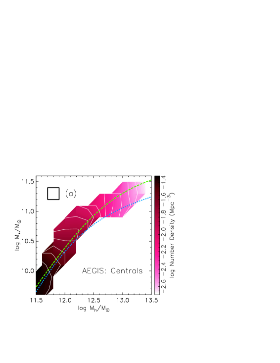
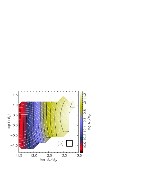
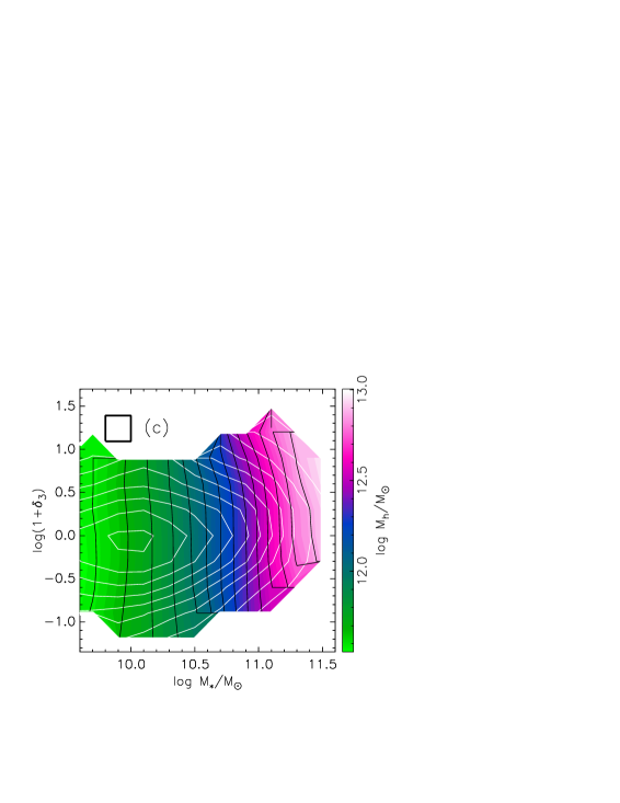
Figure 12: (a). Stellar mass $M_{\rm*}$ versus halo mass $M_{\rm h}$ for the AEGIS ($0.75<z<1$). The green dashed curve is a fit to Eq. 7 of Yang et al. (2008). The blue dotted line is the analogous fit for the SDSS. (b) Mean stellar mass $M_{\rm*}$ as a function of density $\delta_{3}$ and halo mass $M_{\rm h}$. (c). Mean halo mass $M_{\rm h}$ as a function of density $\log(1+\delta_{3})$ and stellar mass $M_{\rm*}$. All panels show only central galaxies in the AEGIS sample. The thin white contours in each panel mark the weighted number density of points and are separated by 0.1 dex in density. The black contours in (b) and (c) follow the coloured shading and are separated by 0.1 dex. The number densities in (a) and the means in (b) and (c) were computed in pixels of the displayed size and smoothed over adjacent pixels. The $M_{\rm*}$-$M_{\rm h}$ relation for massive centrals at $z\sim 1$ lands higher than that of the centrals at $z\sim 0$, consistent with halo growth since $z\sim 1$. $\delta_{3}$ and $M_{\rm h}$ do not correlate except that centrals of massive haloes do not live in sparce environments.

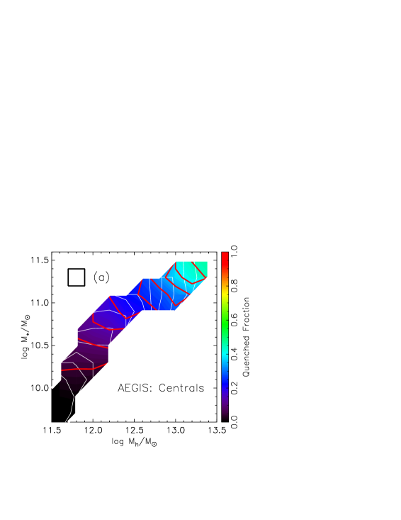
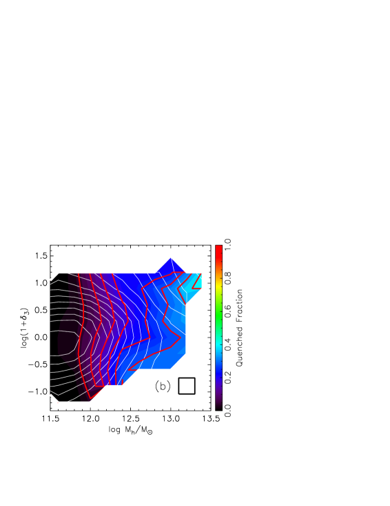
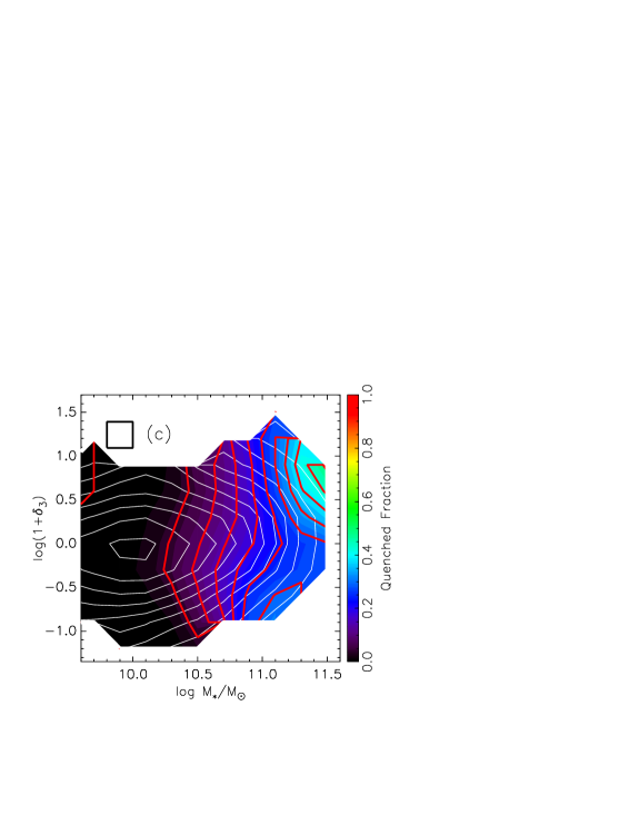
Figure 13: The mean quenched fraction as a function of $M_{\rm*}$ and $M_{\rm h}$ (a), of $\delta_{3}$ and $M_{\rm h}$ (b), and of $\delta_{3}$ and $M_{\rm*}$ (c) for central galaxies in the AEGIS ($0.75<z<1$). The thin white contours mark the weighted number density of points and are separated by 0.1 dex in density. The red (dark) contours follow the coloured shading and are separated by 0.05. The means were computed in pixels of the displayed size and smoothed over adjacent pixels. Below $M_{\rm h}\sim 10^{12.5}{\rm M}_{\odot}$, quenching for centrals at $z\sim 1$ increases primarily with $M_{\rm*}$. Above this mass, quenching increases with $\delta_{3}$, corresponding with the increase of $M_{\rm h}$ with $\delta_{3}$ in Fig. 12$c$ just as for the SDSS centrals. But the overall quenched fraction remains low.

As we have argued, halo quenching via virial shock seems to dominate the quenching of galaxies in haloes above $M_{\rm h}\sim 10^{12.5}{\rm M}_{\odot}$, i.e., those that are large enough to support a virial shock. However, haloes smaller than this are less likely to support a stable virial shock and such haloes would be ideal for testing whether non-halo-dependent quenching mechanisms operate when virial shock heating is relatively unimportant. As described above, the majority (85$\%$) of galaxies at $z\sim 1$ reside in haloes smaller than $M_{\rm h}\sim 10^{12.5}{\rm M}_{\odot}$ (corresponding to $M_{\rm*}\sim 10^{11}{\rm M}_{\odot}$ for centrals - see Fig. 12$a$) while the stellar mass function of galaxies has remained relatively constant over time since $z\sim 1$ (e.g., Bundy et al., 2006). While the halo quenching model predicts very low quenched fractions at all masses below $M_{\rm h}\sim 10^{12.5}{\rm M}_{\odot}$, the behaviour of the quenched fraction in this regime will indicate the strength of other quenching mechanisms when halo quenching is expected to be less important.

Fig. 13 shows the same panels as Fig. 12 (i.e., central galaxies at $z\sim 1$) with the quenched fraction as the third parameter denoted by the coloured shading. Panel $a$ shows that the quenched fraction depends only on $M_{\rm*}$ (horizontal red lines) for low-mass centrals but begins to depend also on $M_{\rm h}$ at higher masses (tilted red lines). The increase of the quenched fraction with $M_{\rm*}$ right below $M_{\rm h}\sim 10^{12.5}{\rm M}_{\odot}$ reflects a similar behaviour at $z\sim 0$ (see Fig. 8$a$ at the lowest masses) and points to an $M_{\rm*}$-dependent quenching mechanism that operates where halo quenching is not expected to dominate.

Note that our AEGIS sample is complete only down to $M_{\rm*}\sim 10^{10.7}{\rm M}_{\odot}$ (Noeske et al., 2007), and the missing galaxies below this mass are likely to be red or quiescent and of lower mass. Therefore, for fixed $M_{\rm h}$ in Fig. 13$a$, regions of lower $M_{\rm*}$ in the incomplete region may actually be more quenched than observed. In other words, the quenching contours in Fig. 13$a$ may in reality be more tilted than horizontal. However we do not expect the effect to be very large since there is evidence (e.g., Bell et al., 2004; Brown et al., 2007; Faber et al., 2007) that there are fewer red galaxies at $z\sim 1$ to be missed at all.

In panel $c$ of Fig. 13, the quenched fraction increases with $M_{\rm*}$ for centrals less massive than $M_{\rm*}\sim 10^{11}{\rm M}_{\odot}$, but begins to increase also with $\log(1+\delta_{3})$ above this mass. For these galaxies the increase of the quenched fraction with $\delta_{3}$ coincides with an increase in $M_{\rm h}$ (Fig. 12$c$) similar to what we saw for the SDSS centrals (§5.1).

In order to ensure that the $M_{\rm*}$-dependence of quenching we observe here is not due some artefact of the group finding process, i.e., contamination by satellites, we tested the AEGIS mock catalogues in the following simple manner. For each mock catalogue, we assumed a mass-independent quenching such that 20% of all centrals and 80% of all satellites are quenched regardless of $M_{\rm*}$ or $M_{\rm h}$. We then computed the quenched fraction in 10 bins of $M_{\rm*}$ and $M_{\rm h}$ for centrals as determined by the group finder. The Pearson correlation coefficients between the quenched fraction and mass were on average $0.02\pm 0.08$ for the quenched fraction vs. $M_{\rm*}$ and $0.14\pm 0.08$ for the quenched fraction vs. $M_{\rm h}$. For the real AEGIS data, the Pearson correlation coefficients are about 0.9 between the quenched fraction and both $M_{\rm*}$ and $M_{\rm h}$. In other words, satellite contamination in the quenching trends is too low to explain the quenching correlations with mass seen in Fig. 13.

Regardless of these trends of the quenched fraction, the total quenched fraction remains low at all masses. The weighted quenched fraction for all the centrals at ($0.75<z<1$) is 0.11. Since the DEEP2 $R$-band magnitude limit corresponds to a lower $M_{\rm*}$ for blue galaxies than red galaxies, we compare these weighted quenched fractions with those of the SDSS after applying a completeness cut that samples the same complete region of colour-mass space out to $z=1$ (refer to Gerke et al., 2007 for details). The colour-mass-complete weighted quenched fraction is 0.41 for centrals, almost four times those of the AEGIS galaxies. This dearth of quenched galaxies at $z\sim 1$ compared to $z\sim 0$ is consistent with the growth of the red sequence over the last $\sim 7$ Gyr (e.g., Bell et al., 2004; Brown et al., 2007; Faber et al., 2007). Since the halo mass function is predicted to have grown an order of magnitude in mass since $z\sim 1$, the quadrupling of the colour-mass-complete quenched fraction from $z\sim 1$ to $z\sim 0$ can naturally be explained by halo mass dependent quenching.

Our result that $M_{\rm*}$-dependent quenching dominates over $M_{\rm h}$- and $\delta_{3}$-dependent quenching for centrals at $z\sim 1$ is consistent with the predictions of McGee et al. (2009). These authors used a semi-analytic model to predict that the fraction of “environmentally affected” galaxies should be very low at $z\sim 1.5$.

Although $M_{\rm*}$-dependent quenching seems to operate in regimes where virial shock heating is expected to be unimportant, it seems to be a weak effect compared to the halo quenching which seems to have eventually overtaken $M_{\rm*}$-dependent quenching by $z\sim 0$.

7 Summary and Conclusions

Using the large sample size of the SDSS at $z\sim 0$ and the multi-wavelength nature of the AEGIS dataset at $z\sim 1$ we have examined the relations between stellar mass, halo mass, environment density and distance of satellites from the group centre over the redshift range $0\ {\raise-2.15277pt\hbox{$\buildrel<\over{\sim}$}}\ z\ {\raise-2.15277pt\hbox{$\buildrel<\over{\sim}$}}\ 1$. We showed that there are two keys to understanding these relations. First, the density estimator to the $N$th-nearest neighbour behaves in two modes, one in which the number of observed group members is less than $N$ so that the density measures the distance to the nearest haloes, and the other in which the number is greater than $N$ so that the density measures distances within a given halo. These are the cross-halo and single-halo modes respectively, and they are typically $\delta_{N}\ll 1$ and $\delta_{N}\gg 1$ for a given $M_{\rm*}$. Second, the relations between $M_{\rm*}$, $M_{\rm h}$ and $\delta_{N}$ behave differently for satellites than for central galaxies. We argued that for satellites, the projected distance from the halo centre $D$, which anti-correlates with $\delta_{N}$ in the single-halo mode, is a better measure of “environment” than $\delta_{N}$ because the former does not behave in two modes that depend on both $N$ and the limiting magnitude of the survey. $D$ measures density, but also time spent in the cluster.

Armed with the understanding of these relations, we explored quenching as a function of the quantities $M_{\rm h}$, $M_{\rm*}$, $\delta_{N}$, and $D$. We used the wealth of SFR data from the SDSS and the AEGIS surveys to measure quenching as the fraction of low-SFR galaxies, rather than the fraction of red galaxies which can be severely affected by dust. We separated the analysis into samples of central and satellite galaxies since the predictions for the behaviour of the quenched fraction differ for these populations.

We also discussed the effects of the halo mass function at $z\sim 1$ having fewer massive haloes compared to $z\sim 0$ on the relations between $M_{\rm*}$, $M_{\rm h}$ and $\delta_{N}$, and on the behaviour of the quenched fraction as a function of these quantities.

Our main results are listed in detail below:

1. Colour: an imperfect surrogate for quenching

   About one third (30% - volume weighted) of the red sequence of the colour-magnitude diagram for the SDSS lies on the SF sequence. These dusty red star forming galaxies tend to be the most massive star forming galaxies and are on average 0.4 dex more massive than the whole population of SF sequence galaxies (see Fig. 3 and the discussion in §3). These results are consistent with those of Maller et al. (2009) who find that a third of red sequence galaxies move to the blue cloud after an inclination-dependent dust correction, and that this dust correction is larger for galaxies with brighter $M_{K}$. The presence of dust-reddened galaxies on the red sequence means that colour does not correlate perfectly with star-formation quenching, which we showed has important implications for quenching correlations vs. stellar and halo mass. For both centrals and satellites, the red fraction will appear to correlate more with $M_{\rm*}$ (due to the massiveness of dusty star formers) and not much with $M_{\rm h}$ (due to the weak correlation between $M_{\rm*}$ and $M_{\rm h}$ at the high end for centrals and no correlation at all for satellites), which is the opposite of the behaviour of the quenched fraction (see Fig. 11 and the discussion in §5.3).

2. Relations between $M_{\rm h}$, $M_{\rm*}$, $\delta_{N}$ and $D$

   1. Environment density as measured by $\delta_{N}$, i.e., the density based on the distance to the $N$th nearest neighbour, is characterised by two modes of behaviour, a cross-halo mode in which the number of observed group members is fewer than $N$ and a single-halo mode where the membership is greater than $N$.

   2. For central galaxies at $z\sim 0$, $M_{\rm*}$ correlates with $M_{\rm h}$ below about $M_{\rm h}\sim{\rm few}\times 10^{12}{\rm M}_{\odot}$ above which $M_{\rm*}$ only weakly depends on $M_{\rm h}$, consistent with the findings of Yang et al. (2009) (Fig. 4$a$). At $z\sim 1$, the relation between $M_{\rm*}$ and $M_{\rm h}$ coincides with the relation at $z\sim 0$ at $M_{\rm h}\sim 10^{12}{\rm M}_{\odot}$, but rises above the $z\sim 0$ relation for haloes more massive than that (Fig. 12$a$). This is consistent with findings of Leauthaud et al. (2012), and with halo growth around central galaxies which grow very little in $M_{\rm*}$. Most (85$\%$) of all galaxies at $z\sim 1$ reside in haloes smaller than $M_{\rm h}=10^{12.5}{\rm M}_{\odot}$.

   3. Central galaxies in the single-halo mode at $z\sim 0$ are characterised by high $\delta_{5}$ and high $M_{\rm h}$, while those in the cross-halo mode exhibit little relation between $\delta_{5}$ and $M_{\rm h}$ (Fig. 4$b$). Central galaxies at $z\sim 1$ behave similarly, but the number of observed group members rarely exceeds $N=3$ (Fig. 12$b$).

   4. For satellite galaxies at $z\sim 0$ in the single-halo mode (which is 58$\%$ of these satellites), $M_{\rm*}$ does not strongly correlate with $M_{\rm h}$. In the cross-halo mode for satellites, $M_{\rm*}$ correlates with $M_{\rm h}$ as expected from statistical and dynamical friction constraints (Fig. 5$b$,$c$).

   5. For satellite galaxies in the single-halo mode at $z\sim 0$, $\delta_{5}$ correlates with $M_{\rm h}$ (Fig. 5$b$), as expected from considerations of the universal halo profile and from the predictions of the spherical collapse model of a virialised halo combined with the known halo occupation function.

   6. For satellites at $z\sim 0$, $\delta_{5}$ anti-correlates with $D=d_{\rm proj}/R_{\rm vir}$ in the single-halo mode but shows no dependence in the cross-halo mode (Fig. 6). This is consistent with the expected statistical behaviour of $\delta_{5}$.

3. Quenching, Mass, Density and Distance

   1. For central galaxies at $z\sim 0$, the quenched fraction appears more strongly correlated with $M_{\rm h}$ (at fixed $M_{\rm*}$) than with $M_{\rm*}$ (at fixed $M_{\rm h}$) for centrals more massive than $M_{\rm*}\sim 10^{10.4}{\rm M}_{\odot}$ (Fig. 8$a$).

   2. At $z\sim 1$, where most of the galaxies reside in haloes less massive than the halo-quenching scale, quenching correlates with $M_{\rm*}$ rather than $M_{\rm h}$ for haloes below $\sim 10^{12.5}{\rm M}_{\odot}$ (which host 85% of these centrals), but the quenched fraction remains low ($\ {\raise-2.15277pt\hbox{$\buildrel<\over{\sim}$}}\ 0.2$) (Fig. 13$a$). This behaviour may signal a $M_{\rm*}$-dependent quenching mode at high redshift that is overtaken by $M_{\rm h}$-dependent quenching as the haloes grow by $z\sim 0$.

   3. For central galaxies at $z\sim 0$, in the $\delta_{5}$-$M_{\rm*}$ plane, the quenched fraction increases with both $M_{\rm*}$ and $\delta_{5}$ (especially at high $M_{\rm*}$) in such a way that is consistent with the increase in mean $M_{\rm h}$ with both of these quantities (compare Fig. 8$c$ with Fig. 4$c$). In other words, the increase of quenching with both $M_{\rm*}$ and $\delta_{5}$ for centrals largely reflects the increase of quenching with $M_{\rm h}$ alone. At $z\sim 1$ the central galaxies behave in a similar way (compare Fig. 13$c$ with Fig. 12$c$).

   4. For satellite galaxies at $z\sim 0$, the quenched fraction increases with $M_{\rm h}$ and decreases with the distance to the group centre $D$ (Fig. 10$a$). The combination of $M_{\rm h}$ and $D$ is an excellent predictor of quenching for satellites, producing quenched fractions as high as 95%. $M_{\rm h}$ and $D$ are preferred over $M_{\rm*}$ and $\delta_{5}$ as predictors of quenching because 1) $\delta_{5}$ behaves differently in two modes and suffers from redshift effects making quenching trends with $\delta_{5}$ difficult to interpret, and 2) quenching follows average $M_{\rm h}$ better than average $M_{\rm*}$ (compare Fig. 9$c$ with Fig. 5$c$ and Fig. 9$b$ with Fig. 5$c$). $M_{\rm*}$-dependent quenching seems to matter more than $M_{\rm h}$ only at large distances from the group centre (where satellites are likely to have just recently fallen in) and may reflect a quenching dependence on the mass of the sub-halo (compare Fig. 10$a$ with $b$). But nearer to the group centre than $\sim 0.2R_{\rm vir}$, the quenching depends strongly on host $M_{\rm h}$ and almost not at all on satellite $M_{\rm*}$.

Our main conclusion is that the quenched fraction of galaxies at $z=0-1$ seems to be primarily driven by the dark-matter halo mass. This is consistent with the theoretical prediction for an accretion shutdown due to virial shock heating once the halo grows above a threshold mass, which possibly triggers other quenching mechanisms, such as stellar and AGN feedback (Birnboim & Dekel, 2003; Dekel & Birnboim, 2006). For satellite galaxies, the quenching also depends on the proximity to the halo center, which reflects the local density and the history of the satellite within the halo. Stellar mass is only a secondary factor, and $\delta_{N}$ is a poor measure of environment. As discussed in §5.3, our results are consistent with those of previous work (eg., Weinmann et al., 2006a; Blanton & Roweis, 2007; Hansen et al., 2009; Kimm et al., 2009; Wetzel et al., 2012a). Our results can be brought into agreement with the conclusion of Peng et al. (2010, 2011) once stellar mass is substituted by halo mass. The difference is driven by our proper use of SFR rather than color to define quenching, and it has the advantage of unifying all phenomena under a common halo quenching model. However, marginal evidence is also found for an $M_{\rm*}$-related quenching mode at earlier epochs when $M_{\rm h}$ is low. It will be valuable to study the quenching mechanism with comparisons to galaxy properties beyond $M_{\rm*}$, such as bulge-to-disk ratio and central density (Cheung et al., Fang et al. and Barro et al., in preparation). Combined with the accretion shutdown associated with halo mass, internal mechanisms related to the bulge and the central black hole may serve as the direct cause for shutdown in star formation (Dekel et al., 2009; Martig et al., 2009).

References

- Abadi et al. (1999) Abadi M. G., Moore B., Bower R. G., 1999, MNRAS, 308, 947
- Adelman-McCarthy et al. (2008) Adelman-McCarthy J. K., et al., 2008, ApJS, 175, 297
- Baldry et al. (2006) Baldry I. K., Balogh M. L., Bower R. G., Glazebrook K., Nichol R. C., Bamford S. P., Budavari T., 2006, MNRAS, 373, 469
- Baldry et al. (2004) Baldry I. K., Glazebrook K., Brinkmann J., Ivezić Ž., Lupton R. H., Nichol R. C., Szalay A. S., 2004, ApJ, 600, 681
- Balogh et al. (2004) Balogh M. L., Baldry I. K., Nichol R., Miller C., Bower R., Glazebrook K., 2004, ApJ, 615, L101
- Balogh et al. (2000) Balogh M. L., Navarro J. F., Morris S. L., 2000, ApJ, 540, 113
- Bamford et al. (2009) Bamford S. P., et al., 2009, MNRAS, 393, 1324
- Bell et al. (2003) Bell E. F., McIntosh D. H., Katz N., Weinberg M. D., 2003, ApJS, 149, 289
- Bell et al. (2004) Bell E. F., et al., 2004, ApJ, 608, 752
- Bell et al. (2005) Bell E. F., et al., 2005, ApJ, 625, 23
- Berlind et al. (2005) Berlind A. A., Blanton M. R., Hogg D. W., Weinberg D. H., Davé R., Eisenstein D. J., Katz N., 2005, ApJ, 629, 625
- Bessell (1990) Bessell M. S., 1990, PASP, 102, 1181
- Binney & Tremaine (1987) Binney J., Tremaine S., 1987, Galactic Dynamics. Princeton, NJ, Princeton University Press, 1987, 747 p.
- Birnboim & Dekel (2003) Birnboim Y., Dekel A., 2003, MNRAS, 345, 349
- Birnboim et al. (2007) Birnboim Y., Dekel A., Neistein E., 2007, MNRAS, 380, 339
- Blanton & Berlind (2007) Blanton M. R., Berlind A. A., 2007, ApJ, 664, 791
- Blanton et al. (2005a) Blanton M. R., Eisenstein D., Hogg D. W., Schlegel D. J., Brinkmann J., 2005a, ApJ, 629, 143
- Blanton & Roweis (2007) Blanton M. R., Roweis S., 2007, AJ, 133, 734
- Blanton et al. (2003) Blanton M. R., et al., 2003, AJ, 125, 2348
- Blanton et al. (2005b) Blanton M. R., et al., 2005b, AJ, 129, 2562
- Brammer et al. (2009) Brammer G. B., et al., 2009, ApJ, 706, L173
- Brinchmann et al. (2004) Brinchmann J., Charlot S., White S. D. M., Tremonti C., Kauffmann G., Heckman T., Brinkmann J., 2004, MNRAS, 351, 1151
- Brown et al. (2007) Brown M. J. I., Dey A., Jannuzi B. T., Brand K., Benson A. J., Brodwin M., Croton D. J., Eisenhardt P. R., 2007, ApJ, 654, 858
- Bruzual & Charlot (2003) Bruzual G., Charlot S., 2003, MNRAS, 344, 1000
- Bundy et al. (2006) Bundy K., et al., 2006, ApJ, 651, 120
- Cacciato et al. (2009) Cacciato M., van den Bosch F. C., More S., Li R., Mo H. J., Yang X., 2009, MNRAS, 394, 929
- Carter et al. (2001) Carter B. J., Fabricant D. G., Geller M. J., Kurtz M. J., McLean B., 2001, ApJ, 559, 606
- Cattaneo et al. (2007) Cattaneo A., et al., 2007, MNRAS, 377, 63
- Chary & Elbaz (2001) Chary R., Elbaz D., 2001, ApJ, 556, 562
- Choi et al. (2009) Choi J.-H., Weinberg M. D., Katz N., 2009, MNRAS, 400, 1247
- Coil et al. (2004) Coil A. L., Newman J. A., Kaiser N., Davis M., Ma C.-P., Kocevski D. D., Koo D. C., 2004, ApJ, 617, 765
- Cooper et al. (2005) Cooper M. C., Newman J. A., Madgwick D. S., Gerke B. F., Yan R., Davis M., 2005, ApJ, 634, 833
- Cooper et al. (2009) Cooper M. C., Newman J. A., Yan R., 2009, ApJ, 704, 687
- Cooper et al. (2006) Cooper M. C., et al., 2006, MNRAS, 370, 198
- Cooper et al. (2008) Cooper M. C., et al., 2008, MNRAS, 383, 1058
- Cooper et al. (2010) Cooper M. C., et al., 2010, MNRAS, 409, 337
- Cooper et al. (2011) Cooper M. C., et al., 2011, ApJS, 193, 14
- Cooper et al. (2012) Cooper M. C., et al., 2012, MNRAS, 419, 3018
- Cooray & Milosavljević (2005) Cooray A., Milosavljević M., 2005, ApJ, 627, L85
- Croton et al. (2006) Croton D. J., et al., 2006, MNRAS, 365, 11
- Davis & Geller (1976) Davis M., Geller M. J., 1976, ApJ, 208, 13
- Davis et al. (2003) Davis M., et al., 2003, in Society of Photo-Optical Instrumentation Engineers (SPIE) Conference Series, Vol. 4834, Society of Photo-Optical Instrumentation Engineers (SPIE) Conference Series, P. Guhathakurta, ed., pp. 161–172
- Davis et al. (2007) Davis M., et al., 2007, ApJ, 660, L1
- De Lucia et al. (2012) De Lucia G., Weinmann S., Poggianti B. M., Aragón-Salamanca A., Zaritsky D., 2012, MNRAS, 3042
- Dekel & Birnboim (2006) Dekel A., Birnboim Y., 2006, MNRAS, 368, 2
- Dekel & Birnboim (2008) Dekel A., Birnboim Y., 2008, MNRAS, 383, 119
- Dekel et al. (2009) Dekel A., Sari R., Ceverino D., 2009, ApJ, 703, 785
- Dekel & Silk (1986) Dekel A., Silk J., 1986, ApJ, 303, 39
- Diaferio et al. (2000) Diaferio A., Sunyaev R. A., Nusser A., 2000, ApJ, 533, L71
- Dressler (1980) Dressler A., 1980, ApJ, 236, 351
- Dressler & Gunn (1983) Dressler A., Gunn J. E., 1983, ApJ, 270, 7
- Dutton et al. (2011) Dutton A. A., et al., 2011, MNRAS, 410, 1660
- Eisenstein & Hu (1998) Eisenstein D. J., Hu W., 1998, ApJ, 496, 605
- Elbaz et al. (2007) Elbaz D., et al., 2007, A&A, 468, 33
- Faber et al. (2007) Faber S. M., et al., 2007, ApJ, 665, 265
- Fall et al. (2010) Fall S. M., Krumholz M. R., Matzner C. D., 2010, ApJ, 710, L142
- Gerke et al. (2005) Gerke B. F., et al., 2005, ApJ, 625, 6
- Gerke et al. (2007) Gerke B. F., et al., 2007, MNRAS, 376, 1425
- Gerke et al. (2012) Gerke B. F., et al., 2012, ApJ, 751, 50
- Gilbank et al. (2010) Gilbank D. G., Baldry I. K., Balogh M. L., Glazebrook K., Bower R. G., 2010, MNRAS, 405, 2594
- Gómez et al. (2003) Gómez P. L., et al., 2003, ApJ, 584, 210
- Granato et al. (2004) Granato G. L., De Zotti G., Silva L., Bressan A., Danese L., 2004, ApJ, 600, 580
- Grützbauch et al. (2011) Grützbauch R., Conselice C. J., Varela J., Bundy K., Cooper M. C., Skibba R., Willmer C. N. A., 2011, MNRAS, 411, 929
- Gunn & Gott (1972) Gunn J. E., Gott, III J. R., 1972, ApJ, 176, 1
- Haas et al. (2012) Haas M. R., Schaye J., Jeeson-Daniel A., 2012, MNRAS, 419, 2133
- Haines et al. (2007) Haines C. P., Gargiulo A., La Barbera F., Mercurio A., Merluzzi P., Busarello G., 2007, MNRAS, 381, 7
- Hansen et al. (2009) Hansen S. M., Sheldon E. S., Wechsler R. H., Koester B. P., 2009, ApJ, 699, 1333
- Hogg et al. (2003) Hogg D. W., et al., 2003, ApJ, 585, L5
- Im et al. (2001) Im M., Faber S. M., Gebhardt K., Koo D. C., Phillips A. C., Schiavon R. P., Simard L., Willmer C. N. A., 2001, AJ, 122, 750
- Kauffmann et al. (2004) Kauffmann G., White S. D. M., Heckman T. M., Ménard B., Brinchmann J., Charlot S., Tremonti C., Brinkmann J., 2004, MNRAS, 353, 713
- Kauffmann et al. (2003) Kauffmann G., et al., 2003, MNRAS, 341, 33
- Kennicutt (1998) Kennicutt R. C., 1998, ARA&A, 36, 189
- Kereš et al. (2005) Kereš D., Katz N., Weinberg D. H., Davé R., 2005, MNRAS, 363, 2
- Kimm et al. (2009) Kimm T., et al., 2009, MNRAS, 394, 1131
- Kong et al. (2004) Kong X., Charlot S., Brinchmann J., Fall S. M., 2004, MNRAS, 349, 769
- Kormendy & Bender (2012) Kormendy J., Bender R., 2012, ApJS, 198, 2
- Kroupa (2001) Kroupa P., 2001, MNRAS, 322, 231
- Larson et al. (1980) Larson R. B., Tinsley B. M., Caldwell C. N., 1980, ApJ, 237, 692
- Le Floc’h et al. (2005) Le Floc’h E., et al., 2005, ApJ, 632, 169
- Leauthaud et al. (2011) Leauthaud A., Tinker J., Behroozi P. S., Busha M. T., Wechsler R. H., 2011, ApJ, 738, 45
- Leauthaud et al. (2012) Leauthaud A., et al., 2012, ApJ, 744, 159
- Lin et al. (1999) Lin H., Yee H. K. C., Carlberg R. G., Morris S. L., Sawicki M., Patton D. R., Wirth G., Shepherd C. W., 1999, ApJ, 518, 533
- Lotz et al. (2008) Lotz J. M., et al., 2008, ApJ, 672, 177
- Lupton et al. (1999) Lupton R. H., Gunn J. E., Szalay A. S., 1999, AJ, 118, 1406
- Maller et al. (2009) Maller A. H., Berlind A. A., Blanton M. R., Hogg D. W., 2009, ApJ, 691, 394
- Mandelbaum et al. (2009) Mandelbaum R., Li C., Kauffmann G., White S. D. M., 2009, MNRAS, 393, 377
- Marcillac et al. (2008) Marcillac D., et al., 2008, ApJ, 675, 1156
- Marinoni & Piazza (2003) Marinoni C., Piazza F., 2003, ArXiv Astrophysics e-prints
- Martig et al. (2009) Martig M., Bournaud F., Teyssier R., Dekel A., 2009, ApJ, 707, 250
- McGee et al. (2009) McGee S. L., Balogh M. L., Bower R. G., Font A. S., McCarthy I. G., 2009, MNRAS, 400, 937
- Miller et al. (2005) Miller C. J., et al., 2005, AJ, 130, 968
- Moore et al. (1996) Moore B., Katz N., Lake G., Dressler A., Oemler A., 1996, Nature, 379, 613
- Moore et al. (1998) Moore B., Lake G., Katz N., 1998, ApJ, 495, 139
- More et al. (2009) More S., van den Bosch F. C., Cacciato M., 2009, MNRAS, 392, 917
- More et al. (2011) More S., van den Bosch F. C., Cacciato M., Skibba R., Mo H. J., Yang X., 2011, MNRAS, 410, 210
- Mostek et al. (2012) Mostek N., Coil A. L., Moustakas J., Salim S., Weiner B. J., 2012, ApJ, 746, 124
- Moster et al. (2010) Moster B. P., Somerville R. S., Maulbetsch C., van den Bosch F. C., Macciò A. V., Naab T., Oser L., 2010, ApJ, 710, 903
- Muldrew et al. (2012) Muldrew S. I., et al., 2012, MNRAS, 419, 2670
- Navarro et al. (1997) Navarro J. F., Frenk C. S., White S. D. M., 1997, ApJ, 490, 493
- Newman et al. (2012) Newman J. A., et al., 2012, ArXiv e-prints
- Noeske (2012) Noeske K., 2012, in American Astronomical Society Meeting Abstracts, Vol. 220, American Astronomical Society Meeting Abstracts, p. 421.01
- Noeske et al. (2007) Noeske K. G., et al., 2007, ApJ, 660, L43
- Oemler (1974) Oemler A. J., 1974, ApJ, 194, 1
- Padmanabhan et al. (2008) Padmanabhan N., et al., 2008, ApJ, 674, 1217
- Peng et al. (2011) Peng Y., Lilly S. J., Renzini A., Carollo M., 2011, ArXiv e-prints
- Peng et al. (2010) Peng Y., et al., 2010, ApJ, 721, 193
- Press & Schechter (1974) Press W. H., Schechter P., 1974, ApJ, 187, 425
- Quadri et al. (2012) Quadri R. F., Williams R. J., Franx M., Hildebrandt H., 2012, ApJ, 744, 88
- Quintero et al. (2004) Quintero A. D., et al., 2004, ApJ, 602, 190
- Read et al. (2006) Read J. I., Wilkinson M. I., Evans N. W., Gilmore G., Kleyna J. T., 2006, MNRAS, 366, 429
- Rines et al. (2005) Rines K., Geller M. J., Kurtz M. J., Diaferio A., 2005, AJ, 130, 1482
- Salim et al. (2007) Salim S., et al., 2007, ApJS, 173, 267
- Salim et al. (2009) Salim S., et al., 2009, ApJ, 700, 161
- Schiminovich et al. (2007) Schiminovich D., et al., 2007, ApJS, 173, 315
- Seibert et al. (2005) Seibert M., et al., 2005, ApJ, 619, L55
- Skibba (2009) Skibba R. A., 2009, MNRAS, 392, 1467
- Skibba & Sheth (2009) Skibba R. A., Sheth R. K., 2009, MNRAS, 392, 1080
- Springel et al. (2005) Springel V., Di Matteo T., Hernquist L., 2005, MNRAS, 361, 776
- Springel et al. (2001) Springel V., White S. D. M., Tormen G., Kauffmann G., 2001, MNRAS, 328, 726
- Strateva et al. (2001) Strateva I., et al., 2001, AJ, 122, 1861
- Tanaka et al. (2004) Tanaka M., Goto T., Okamura S., Shimasaku K., Brinkmann J., 2004, AJ, 128, 2677
- Tinker et al. (2008) Tinker J., Kravtsov A. V., Klypin A., Abazajian K., Warren M., Yepes G., Gottlöber S., Holz D. E., 2008, ApJ, 688, 709
- Tremonti et al. (2004) Tremonti C. A., et al., 2004, ApJ, 613, 898
- van den Bosch et al. (2008) van den Bosch F. C., Pasquali A., Yang X., Mo H. J., Weinmann S., McIntosh D. H., Aquino D., 2008, ArXiv e-prints
- Villalobos et al. (2012) Villalobos Á., De Lucia G., Borgani S., Murante G., 2012, ArXiv e-prints
- von der Linden et al. (2010) von der Linden A., Wild V., Kauffmann G., White S. D. M., Weinmann S., 2010, MNRAS, 404, 1231
- Warren et al. (2006) Warren M. S., Abazajian K., Holz D. E., Teodoro L., 2006, ApJ, 646, 881
- Weiner et al. (2007) Weiner B. J., et al., 2007, ApJ, 660, L39
- Weinmann et al. (2010) Weinmann S. M., Kauffmann G., von der Linden A., De Lucia G., 2010, MNRAS, 406, 2249
- Weinmann et al. (2006a) Weinmann S. M., van den Bosch F. C., Yang X., Mo H. J., 2006a, MNRAS, 366, 2
- Weinmann et al. (2006b) Weinmann S. M., van den Bosch F. C., Yang X., Mo H. J., Croton D. J., Moore B., 2006b, MNRAS, 372, 1161
- Wetzel et al. (2012a) Wetzel A. R., Tinker J. L., Conroy C., 2012a, MNRAS, 3128
- Wetzel et al. (2012b) Wetzel A. R., Tinker J. L., Conroy C., van den Bosch F. C., 2012b, ArXiv e-prints
- Willmer et al. (2006) Willmer C. N. A., et al., 2006, ApJ, 647, 853
- Wilman et al. (2010) Wilman D. J., Zibetti S., Budavári T., 2010, MNRAS, 406, 1701
- Wolf et al. (2009) Wolf C., et al., 2009, MNRAS, 393, 1302
- Yan et al. (2004) Yan R., White M., Coil A. L., 2004, ApJ, 607, 739
- Yang et al. (2008) Yang X., Mo H. J., van den Bosch F. C., 2008, ApJ, 676, 248
- Yang et al. (2009) Yang X., Mo H. J., van den Bosch F. C., 2009, ApJ, 695, 900
- Yang et al. (2007) Yang X., Mo H. J., van den Bosch F. C., Pasquali A., Li C., Barden M., 2007, ApJ, 671, 153
- Yang et al. (2012) Yang X., Mo H. J., van den Bosch F. C., Zhang Y., Han J., 2012, ApJ, 752, 41
- York et al. (2000) York D. G., et al., 2000, AJ, 120, 1579