The Exoplanet Eccentricity Distribution from Kepler Planet Candidates

Abstract

The eccentricity distribution of exoplanets is known from radial velocity surveys to be divergent from circular orbits beyond 0.1 AU. This is particularly the case for large planets where the radial velocity technique is most sensitive. The eccentricity of planetary orbits can have a large effect on the transit probability and subsequently the planet yield of transit surveys. The Kepler mission is the first transit survey that probes deep enough into period-space to allow this effect to be seen via the variation in transit durations. We use the Kepler planet candidates to show that the eccentricity distribution is consistent with that found from radial velocity surveys to a high degree of confidence. We further show that the mean eccentricity of the Kepler candidates decreases with decreasing planet size indicating that smaller planets are preferentially found in low-eccentricity orbits.

1 Introduction

Planets discovered using the radial velocity (RV) method have dominated the total exoplanet count until recently, when the transit method has made increasing contributions. The long time baseline of RV surveys has allowed the detection more diverse orbital geometries than achievable by ground-based transit surveys. The Kepler mission, however, with its multi-year baseline, can begin to probe into parameter space previously reserved for RV studies. At longer periods, orbits tend to diverge significantly from the circular case beyond a semi-major axis of $\sim 0.1$ AU (Butler et al., 2006), although there may be small observational biases that skew this distribution (Shen & Turner, 2008). This insight has led to numerous attempts to account for eccentricity in the context of planet formation and orbital stability (Ford & Rasio, 2008; Malmberg & Davies, 2008; Matsumura et al., 2008; Jurić & Tremaine, 2008; Wang & Ford, 2011) and the influence of tidal circularization (Pont et al., 2011).

It has been shown how eccentricity distribution effects transit probabilities (Kane & von Braun, 2008, 2009) and projected yields of transit surveys (Barnes, 2007; Burke, 2008). This influence is minor for the ground-based surveys since they are primarily sensitive to giant planets in short-period orbits. However, the Kepler mission is expected to be impacted by this distribution since it probes out to much longer periods with a much reduced disadvantage of a window function that affects observations from the ground (von Braun et al., 2009). A comparison of the Kepler results in the context of eccentricity and transit durations with the RV distribution has been suggested by Ford et al. (2008) and Zakamska et al. (2011) and carried out by Moorhead et al. (2011), but initial planet candidate releases by the Kepler project do not provide enough period sensitivity (Borucki et al., 2011a, b). The most recent release of Kepler planet candidates by Batalha et al. (2012) increases the total number of candidates to more than 2,300 and the time baseline probed to beyond 560 days. This has several implications for studies of eccentricity distributions. The Kepler mission is sensitive to planets significantly smaller than those accessible by current RV experiments and thus allows a more in-depth study of the dependence of eccentricity on the planet mass/size and multiplicity. If the eccentricity distributions of Kepler and RV planets were found to be substantially different then this may reveal a selection effect in the way Kepler candidates are selected which is biased against eccentric orbits. A direct comparison of the two distributions, provided they are consistent for the planet mass/size region where their sensitivities overlap, will allow a more exhaustive investigation of orbital eccentricity to be undertaken.

Here we present a study of the eccentricity distribution of planets discovered with the RV method and the complete list of Kepler planet candidates. We calculate expected transit durations for circular orbits and compare them with either calculated or measured eccentric transit durations (§2). Our results show that the measured transit durations from RV data (§3) and the Kepler candidates (§4) are consistent with having the same distribution. We estimate the impact parameter distribution for the Kepler candidates and show that their mean eccentricity decreases with decreasing planet size (§5), which supports the hypothesis that smaller planets tend to be found in multiple systems in near-circular orbits. We discuss additional astrophysical aspects in §6 and conclude in §7.

2 Eccentricity and Transit Duration

A concise description of exoplanetary transit modeling and associated parameters is presented elsewhere (Mandel & Agol, 2002; Seager & Mallén-Ornelas, 2002). Here we concentrate on the relevant details to our analysis: transit duration and eccentricity. The transit duration for a circular orbit is given by

$$t_{\mathrm{circ}}=\frac{P}{\pi}\arcsin\left(\frac{\sqrt{(R_{\star}+R_{p})^{2}-a^{2}\cos^{2}i}}{a}\right),$$ (1)

where $P$ is the orbital period, $a$ is the semi-major axis, $i$ is the orbital inclination, and $R_{\star}$ and $R_{p}$ are the stellar and planetary radii respectively. The impact parameter of a transit is given by

$$b\equiv\frac{a}{R_{\star}}\cos i$$ (2)

and is defined as the projected separation of the planet and star centers at the point of mid-transit.

Figure 1: The eccentricity distribution of the known radial velocity planets (top-left) and the calculated transit duration difference (circular vs eccentric) for $b=0.0$ (top-right), 0.5 (bottom-left), and 0.8 (bottom-right). See §3 for details.

For an eccentric orbit, the star–planet separation $r$ is time-dependent and is given by

$$r=\frac{a(1-e^{2})}{1+e\cos f}$$ (3)

where $e$ is the orbital eccentricity and $f$ is the true anomaly. Replacing $a$ with $r$ at the time of inferior conjunction in equations 1 and 2 provides generalized expressions for transit duration and impact parameter for non-circular orbits. Burke (2008) converts these expressions into the scaling factor

$$\frac{t_{\mathrm{ecc}}}{t_{\mathrm{circ}}}=\frac{\sqrt{1-e^{2}}}{1+e\cos(\omega-90\degr)},$$ (4)

where $\omega$ is the periastron argument of the orbit.

3 Radial Velocity Eccentricity Distribution

We first investigate the eccentricity distribution of the planets discovered with the RV technique and the subsequent impact on the predicted transit duration. The Exoplanet Data Explorer (EDE) stores information only for those planets that have complete orbital solutions and thus are well suited to this study (Wright et al., 2011). The EDE data are current as of 2012 February 24 and include 204 planets after the following criteria are applied: $\log g>3.5$ to exclude giant stars and $a<1.5$ AU to produce a sample that covers the same region in parameter space as the Kepler candidates.

To calculate the transit duration, one needs an estimate of the planetary radius. For planets that are not known to transit, we approximate the planetary radius using the simple model described by Kane & Gelino (2012). This model adopts a radius of 1 Jupiter radius for masses $\geq 0.3M_{Jupiter}$ and utilizes a power law fit to the masses and radii of the known transiting planets for masses $<0.3M_{Jupiter}$. In order to estimate the radius of the host star, we use the following relation related to the surface gravity

$$\log g=\log\left(\frac{M_{\star}}{M_{\odot}}\right)-2\log\left(\frac{R_{\star}}{R_{\odot}}\right)+\log g_{\odot}$$ (5)

where $\log g_{\odot}=4.4374$ (Smalley, 2005). Using the equations of Section 2 and the measured orbital parameters, we calculate the transit duration for both the circular and eccentric cases. We then take the absolute value of the difference between the two durations as a diagnostic for the eccentricity distribution.

Figure 2: The calculated transit duration difference (circular vs measured) for the Kepler candidates (left). The cumulative histograms for the Kepler candidates and the three radial velocity planets shown in Figure 1 show a close match between the distributions, quantified by the K-S test described in Section 4.

The top-left panel of Figure 1 shows the eccentricity distribution of the RV planets taken from EDE as a function of $a$. The distribution begins to diverge from mostly circular orbits beyond 0.04 AU, and by 0.1 AU it has an eccentricity range of 0.0–0.5. This distribution is widely attributed to tidal damping of the orbits after the disk has dissipated. According to Goldreich & Soter (1966), the timescale for orbital circularization is $\propto a^{6.5}M_{\star}^{-1.5}$ where $M_{\star}$ is the stellar mass. Note that the two planets inside of 0.04 AU with $e>0.1$ are GJ 436b and GJ 581e, both of which have M dwarf host stars.

The other three panels in Figure 1 show the calculated duration difference by $\Delta t$ as a function of $a$. $\Delta t$ is the absolute value of the difference between the calculated transit duration for a circular orbit and the calculated transit duration based upon the measured orbital parameters (i.e., $\Delta t=|t_{\mathrm{circ}}-t_{\mathrm{ecc}}|$), which is indicative of the divergence from the assumption of only circular orbits. The top-right panel assumes edge-on orbits ($i=90\degr;b=0$) for both the circular and eccentric cases. We show the effect of increasing the impact parameter of the transits for $b=0.5$ and $b=0.8$. The mean of $\Delta t$ is not significantly changed except for relatively high values of $b$. We evaluate the significance of this distribution in the following section.

It should be noted that, in order for a transit to take place, $i$ can at most only slightly deviate from $90\degr$. The consequent small angle approximation means that the uniform distribution of $i$ values maps to a uniform distribution of $b$ values, making all values of $b$ equally likely to occur.

4 Analysis of Kepler Transit Durations

The release of more than 2,300 Kepler candidates is described in detail by Batalha et al. (2012). The appendix table that contains the characteristics of the Kepler candidates was extracted from the NASA Exoplanet Archive. We perform a similar calculation for $\Delta t$ as described in the previous section. However, this time we calculate the difference between $t_{\mathrm{circ}}$ and the duration measurement provided by the candidates table, $t_{\mathrm{kepler}}$. We do not use the provided $b$ values since they are based on a circular orbit assumption from the measured transit duration and the stellar radii. We thus make no assumption on the value of $b$. We require $R_{\star}>0.7R_{\odot}$ to remove candidates for which the uncertainty in the stellar radius determination contributes significantly to the uncertainty in the transit duration. We also only include candidates for which $R_{p}>8R_{\oplus}$ to limit the sample to giant planets, similar to the RV sample. We show $\Delta t$ versus $a$ for the 176 resulting candidates in the left panel of Figure 2.

To compare this distribution to its equivalents in Section 3 we perform a null hypothesis Kolmogorov-Smirnov (K-S) test to assess the statistical significance of their similarities. We binned the data by $\Delta t$ into 40 equal bins of 0.5 to collapse the data into 1-dimensional samples. The right panel of Figure 2 shows the normalized cumulative histograms for each of the four distributions: the three K-S tests compare the Kepler candidates to the RV planets with assumed $b=0.0$ (Test 1), $b=0.5$ (Test 2), and $b=0.8$ (Test 3). Test 1 produces a K-S statistic of $D=0.05$ that indicates a 100% probability that these data are consistent with being drawn from the same distribution (the null hypothesis). Test 2 produces a similar result of $D=0.075$, also a probability of 100%. Test 3 results in $D=0.2$ which is equivalent to a probability of 36%. This result can readily be seen in the right panel of Figure 2 where the $b=0.0$ and $b=0.5$ cases are almost indistinguishable from the Kepler candidates, but the $b=0.8$ case is clearly discrepant. As mentioned in §3, the small range of values for $i$ for transits results in a uniform distribution of impact parameters with a mean of $b=0.5$. The statistical congruence in the K-S test implies that the Kepler Mission is indeed recovering the eccentricity distribution of the RV planets.

A criticism that may be levelled at this methodology is that the outcome of the statistical test depends upon the manner in which the data is binned. To determine the robustness of our results, we used both half and double the number of bins to change the resolution of the sampling. For half the number of bins, we obtain $D=0.1$ (100%), $D=0.1$ (100%), and $D=0.2$ (77%) for Tests 1, 2, and 3 respectively as described above. If we then double the number of bins, the results are $D=0.05$ (100%), $D=0.0375$ (100%), and $D=0.1625$ (22%) for Tests 1, 2, and 3 respectively. Clearly the results for Tests 1 and 2 are consistent with previous results and the results for Test 3 retain their discrepancies though with a variety of values. As described earlier, Test 3 ($b=0.8$) is the least relevant of the results since the mean impact parameter is $b=0.5$.

Table 1: Minimum eccentricities for selected candidates.

KOI	Period	$t_{\mathrm{kepler}}$	$\Delta t$	$e_{\mathrm{min}}$
	(days)	(hours)	(hours)
44.01	66.47	19.74	12.2	0.74
211.01	372.11	4.81	10.5	0.82
625.01	38.14	4.24	10.7	0.85
682.01	562.14	9.49	10.8	0.64
1230.01	165.72	27.26	11.8	0.34
1894.01	5.29	8.80	14.4	0.75
2133.01	6.25	11.26	14.1	0.67
2481.01	33.85	14.95	16.8	0.64

Finally, we investigate a sample of the outliers with particularly large deviations from the circular model ($\Delta t>10$ hours). These candidates are shown in Table 1. Since the Kepler data frequently do not contain any secondary eclipse, $e$ and $\omega$ are unknown. We calculate transit duration $t_{\mathrm{ecc}}$ as a function of $e$ and $\omega$ via Equation 4. We then produce a grid of $|t_{\mathrm{circ}}-t_{\mathrm{kepler}}|/|t_{\mathrm{circ}}-t_{\mathrm{ecc}}|$ for all values of $e$ and $\omega$. Locations where the grid values are approximately equal to 1 are possible solutions for which the measured transit duration in the Kepler candidate catalog is consistent with certain values of $e$ and $\omega$.

An example of this is shown in Figure 3 where we present results of the above calculations as an intensity map for KOI 1230.01. In order to be compatible with the Kepler measured duration, the eccentricity of the planet must be at least 0.34. This process is repeated for each of the candidates in Table 1 in which we report the minimum required eccentricity $e_{\mathrm{min}}$ for each candidate. It is worth noting, however, that these minimum eccentricities are not singular values but rather distributions, as can be seen by the gray-scale in Figure 3. The uncertainties depend highly upon the various random errors in the measured values of the Kepler candidates catalogue, including $i$. For example, the stellar radius of KOI 2481.01 would need to be $\sim 45$% of the catalogue value in order for it to be in a circular orbit and the duration discrepancy to be reduced to zero.

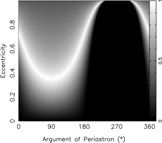
Figure 3: An intensity map for KOI 1230.01 that shows the result of dividing $\Delta t$ using $t_{\mathrm{kepler}}$ by $\Delta t$ using $t_{\mathrm{ecc}}$. Thus, a value of 1 (peak intensity) corresponds to the best solution (§4).

Further of interest in Table 1 are the relatively short-period planets KOI 1894.01 and KOI 2133.01. One normally expects a transit duration of several hours for period such as these. However, the values of $t_{\mathrm{kepler}}$ and $\Delta t$ shown in this table imply a $t_{\mathrm{circ}}$ larger than 20 hours! This does not appear to make sense until one considers the stellar radius. Note from Equation 1 that, for an edge-on orbit and small $R_{p}$, the transit duration scales linearly with the size of the star. For these two candidates, the stellar radii are 8.6 and 9.3 solar radii respectively thus resulting in a large $\Delta t$ and a significant eccentricity required to be consistent with observations. Note, however, that we have assumed $b=0$. As one increases the impact parameter, the predicted transit duration will decrease and thus become closer to its measured value. Results for individual cases extracted from the global distribution, such as those in Table 1, must therefore be treated with caution.

5 Planet Size Correlation

We mentioned in Section 4 that the analysis of the Kepler objects included only candidates for which $R_{p}>8R_{\oplus}$. Here we perform a separate study by repeating the calculations of $\Delta t$ for the Kepler candidates for a range of planetary radii. We allow the candidate sample to include all radii larger than $1R_{\oplus}$ to $8R_{\oplus}$ and calculate the mean of the $\Delta t$ distribution in each case. We show our results in Figure 4.

Figure 4: The mean $\Delta t$ for the Kepler candidates as a function of minimum planetary radius included in the sample (§5).

An interpretation of this figure is that the eccentricity distribution of exoplanets remains relatively flat until we probe below planets the size of Neptune. At that point the eccentricity distribution of the orbits becomes rapidly and significantly more circular. This is not unexpected since we understand from the solar system that the inefficiency of tidal dissipation (the quality factor $Q$) is much larger for high-mass than for low-mass planets (Goldreich & Soter, 1966), resulting in shorter tidal circularization time scales for smaller planets. One aspect of the Kepler candidate sample that may influence this result is that they are dominated by planets at smaller semi-major axes since these have much larger transit probabilities. As indicated by Lissauer et al. (2011b) and Lissauer et al. (2012), multi-planet systems comprise a large proportion of the total Kepler candidate sample and these systems in particular are less prone to be false-positives. The findings that planet occurrence increases with decreasing planet mass (see for example Howard et al., 2010) then suggests that smaller planets find stable architectures in systems with circular orbits and without large planets in eccentric orbits. This lends credence to two scenarios: (1) core accretion forming terrestrial planets in circular orbits, and (2) disk instability and capture scenario explaining the existence of giant planets in eccentric orbits.

A potential alternative explanation for the dependence of $\Delta t$ upon $R_{planet}$ is a correlation between planetary radii and semi-major axes in the Kepler sample due to completeness. Smaller planets in closer orbits would be more likely to have had their orbits circularized leading to their domination of the sample. We do not, however, see such an effect but instead find no correlation between planet size and period in the Kepler catalog for the selected range of orbital periods. Thus, we conclude that this effect is not the cause of the observed radius/eccentricity correlation.

6 Discussion

There are various sources of potential systematic noise inherent in the data used to perform this analysis. For example, we have not taken the stellar limb-darkening into account when considering transit durations. However, since we only consider the total transit duration (first contact to last contact), this will be a negligible effect.

For the Kepler candidates, the primary source of uncertainty arises from the stellar parameters that are used to derive many of the planetary candidate parameters. The primary difficulties arise from the stellar radii whose precision is usually worse than $\sim$10%, even when spectra are available. Our assumption is that these uncertainties are not significantly biased in one direction of the other and thus only add white noise to the overall statistical properties. One method to test this assumption is to consider multi-candidate systems for which a change in the stellar radius will effect all calculated transit durations in a similar way. For example, KOI 157 (Kepler-11) has 6 detected planet candidates with measured transit durations that are shorter than predicted, and with an estimated host star radius of 1.06 $R_{\odot}$. Three of those discrepancies are quite small making them almost consistent with a circular orbit, as noted by Lissauer et al. (2011a). Attempting to force circular orbits by reducing the stellar radius slightly makes 2 of the planets consistent with a circular orbit but leaves the other durations highly discrepant. A more global test of the assumption is the application of a range of uniform scaling factors to the stellar radii to try to produce transit durations consistent with circular orbits for the bulk of the distribution. These corrections did not change the distribution shown in Figure 2, leading to the conclusion that our calculated $\Delta t$ values are not affected by systematically incorrect stellar radii.

Considering the uncertainties in the radii of the Kepler host stars, our limits on the eccentricities of the specific Kepler candidates discussed in Section 4 should be treated in that context. Indeed, this is why we concentrate our comments on the global distribution of all the Kepler objects and their parameters, rather than on individual cases. Furthermore, the Kepler sample is only complete to $\sim 0.5$ AU with declining completeness beyond this to $\sim 1.5$ AU. Thus, the number of candidates beyond 0.5 AU is smaller but still sufficient for a valid comparison to be made.

One aspect of the Kepler candidates that was not taken into account was the multiplicity of the systems. As suggested at the conclusion of the previous section, the multiplicity may indeed play a significant role in stabilizing planets in approximately circular orbits, particularly for those in the low mass/size regime. This is true of the radial velocity planets also, some of which are known to lie in multiple systems of super-Earth mass planets and with relatively circular orbits such as the system orbiting HD 10180 (Lovis et al., 2011).

In Section 1 we mentioned the eccentricity bias found by Shen & Turner (2008) due to low-amplitude signals in RV samples. This is a small but real effect which depends upon the sampling rate and has the consequence of under-estimating the number of near-circular orbits. Shen & Turner (2008) develop a figure-of-merit and find that only $\sim 10$% of the planets considered in their sample are affected by this bias. The samples studied here are two small to detect such an effect, but we mention it here as a consideration for future similar work for which the sample sizes and, more particularly, the period range explored have grown substantially.

Finally, a minor impact on the stellar radii that should be noted is the one due to the relation between planet frequency and stellar metallicity. Johnson et al. (2010) explored the mass-metallicity relationship for stars that harbor planets and found a positive correlation of planet frequency with both stellar mass and metallicity, in accordance with the findings of Fischer & Valenti (2005). This positive correlation was also found empirically for M dwarfs by Terrien et al. (2012). For a given stellar mass, a larger metallicity leads to a smaller radius in order to reach hydrostatic equilibrium. The implication for this study is that many of the Kepler host stars will have relatively high metallicity leading to an over-estimated radius. However, this effect is at the level of a few percent and not expected to interfere with the results of this study.

7 Conclusions

By conducting a transit survey that is sensitive to long enough periods, it is expected that one will eventually reproduce the eccentricity distribution found amongst radial velocity planets. This has not been possible until very recently, when the Kepler presented a large sample of long-period planets candidates, providing the incentive for this study and a similar one by Plavchan et al. (2012). For individual planets, the eccentricity may be discerned via asymmetry in the shape of ingress and egress (Kipping, 2008). This requires exquisite photometry and is highly sensitive to $\omega$. We have shown here the consistency of the Kepler candidates’ eccentricity distribution with their RV planets counterparts. The correlation of eccentricity with planet size is also an expected result based upon the discoveries of small planets in multiple systems and indicates that there is an empirical approach from which to both reverse-engineer formation scenarios and predict future stability patterns.

References

- Barnes (2007) Barnes, J.W., 2007, PASP, 119, 986
- Batalha et al. (2012) Batalha, N.M., et al., 2012, ApJS, submitted (arXiv:1202.5852)
- Borucki et al. (2011a) Borucki, W.J., et al., 2011, ApJ, 728, 117
- Borucki et al. (2011b) Borucki, W.J., et al., 2011, ApJ, 736, 19
- Butler et al. (2006) Butler, R.P., et al., 2006, ApJ, 646, 505
- Burke (2008) Burke, C.J., 2008, ApJ, 679, 1566
- Fischer & Valenti (2005) Fischer, D.A., Valenti, J., 2005, ApJ, 622, 1102
- Ford et al. (2008) Ford, E.B., Quinn, S.N., Veras, D., 2008, ApJ, 678, 1407
- Ford & Rasio (2008) Ford, E.B., Rasio, F.A., 2008, ApJ, 686, 621
- Goldreich & Soter (1966) Goldreich, P., Soter, S., 1966, Icarus, 5, 375
- Howard et al. (2010) Howard, A.W., et al., 2010, Science, 330, 653
- Johnson et al. (2010) Johnson, J.A., Aller, K.M., Howard, A.W., Crepp, J.R., 2010, PASP, 122, 905
- Jurić & Tremaine (2008) Jurić, M., Tremaine, S., 2008, ApJ, 686, 603
- Kane & Gelino (2012) Kane, S.R., Gelino, D.M., 2012, PASP, 124, 323
- Kane & von Braun (2008) Kane, S.R., von Braun, K., 2008, ApJ, 689, 492
- Kane & von Braun (2009) Kane, S.R., von Braun, K., 2009, PASP, 121, 1096
- Kipping (2008) Kipping, D.M., 2008, MNRAS, 389, 1383
- Lissauer et al. (2011a) Lissauer, J.J., et al., 2011, Nature, 470, 53
- Lissauer et al. (2011b) Lissauer, J.J., et al., 2011, ApJS, 197, 8
- Lissauer et al. (2012) Lissauer, J.J., et al., 2012, ApJ, 750, 112
- Lovis et al. (2011) Lovis, C., et al., 2011, A&A, 528, 112
- Malmberg & Davies (2008) Malmberg, D., Davies, M.B., 2009, MNRAS, 394, L26
- Mandel & Agol (2002) Mandel, K., Agol, E., 2002, ApJ, 580, L171
- Matsumura et al. (2008) Matsumura, S., Takeda, G., Rasio, F.A., 2008, ApJ, 686, L29
- Moorhead et al. (2011) Moorhead, A.V., et al., 2011, ApJS, 197, 1
- Plavchan et al. (2012) Plavchan, P., Bilinski, C., Currie, T., 2012, ApJL, submitted (arXiv:1203.1887)
- Pont et al. (2011) Pont, F., Husnoo, N., Mazeh, T., Fabrycky, D., 2011, MNRAS, 414, 1278
- Seager & Mallén-Ornelas (2002) Seager, S., Mallén-Ornelas, G., 2003, ApJ, 585, 1038
- Shen & Turner (2008) Shen, Y., Turner, E.L., 2008, ApJ, 685, 553
- Smalley (2005) Smalley, B., 2005, Mem. Soc. Astron. Ital. Suppl., 8, 130
- Terrien et al. (2012) Terrien, R.C., Mahadevan, S, Bender, C.F., Deshpande, R., Ramsey, L.W., Bochanski, J.J., 2012, ApJ, 747, L38
- von Braun et al. (2009) von Braun, K., Kane, S.R., Ciardi, D.R., 2009, ApJ, 702, 779
- Wang & Ford (2011) Wang, J., Ford, E.B., 2011, MNRAS, 418, 1822
- Wright et al. (2011) Wright, J.T., et al., 2011, PASP, 123, 412
- Zakamska et al. (2011) Zakamska, N.L., Pan, M., Ford, E.B., 2011, MNRAS, 410, 1895