The degeneracy between star-formation parameters in dwarf galaxy simulations and the $M_{\rm star}-M_{\rm halo}$ relation

Abstract

We present results based on a set of N-Body/SPH simulations of isolated dwarf galaxies. The simulations take into account star formation, stellar feedback, radiative cooling and metal enrichment. The dark matter halo initially has a cusped profile, but, at least in these simulations, starting from idealised, spherically symmetric initial conditions, a natural conversion to a core is observed due to gas dynamics and stellar feedback.

A degeneracy between the efficiency with which the interstellar medium absorbs energy feedback from supernovae and stellar winds on the one hand, and the density threshold for star formation on the other, is found. We performed a parameter survey to determine, with the aid of the observed kinematic and photometric scaling relations, which combinations of these two parameters produce simulated galaxies that are in agreement with the observations.

With the implemented physics we are unable to reproduce the relation between the stellar mass and the halo mass as determined by Guo et al. (2010), however we do reproduce the slope of this relation.

1 Introduction

Dwarf galaxies are the most common type of galaxy in the local universe but also the faintest and least easy to observe. In the $\Lambda$CDM cosmology, our universe consists of matter, both luminous and dark, and dark energy, which is responsible for the accelerating expansion of the universe. Galaxies form when gas collapses in dark matter halos. Baryons, be it in the form of gas, dust or stars, are the most accessible form of matter, emitting radiation over the whole electromagnetic spectrum. Dark matter, on the other hand, as it only interacts gravitationally, is much more difficult to “observe”.

There have been many attempts to estimate dark halo masses and mass-to-light ratios for galaxies and clusters of galaxies from direct observations. These include methods that make use of gravitational lensing (Mandelbaum et al., 2006; Liesenborgs et al., 2009), dynamical modeling of the observed properties of a kinematical tracer such as stars or planetary nebulae (Kronawitter et al., 2000; De Rijcke et al., 2006; Napolitano et al., 2011; Barnabè et al., 2009). One thing virtually all these works have in common is the relatively limited size of the data set they are based on. Guo et al. (2010) determined the halo mass as a function of stellar mass for a large sample of galaxies using a statistical analysis of the Sloan Digital Sky Survey, which yields the stellar masses, and the Millennium Simulations, which yield the dark-matter masses. In the range of the most massive halos and bright galaxies, the derived $M_{\rm star}$-$M_{\rm halo}$ relation, which is of the form $M_{\rm star}\propto M_{\rm halo}^{0.36}$, is found to be in good agreement with gravitational lensing data (Mandelbaum et al., 2006). Below a halo mass of $M_{\rm halo}\sim 10^{11.4}$ $M_{\odot}$, this relation becomes much steeper: $M_{\rm star}\propto M_{\rm halo}^{3.26}$. Guo et al. (2010) extrapolate the latter relation into the dwarf regime, where $M_{\rm halo}\lesssim 10^{10}$ $M_{\odot}$. This leads then to the prediction that faint dwarf galaxies with stellar masses of the order of $M_{\rm star}\sim 10^{6}$ $M_{\odot}$ should live in comparatively massive $M_{\rm halo}\sim 10^{10}$ $M_{\odot}$ dark-matter halos.

The Guo et al. (2010) $M_{\rm star}$-$M_{\rm halo}$ relation was compared with that found in simulations of dwarf galaxies (Valcke et al., 2008; Stinson et al., 2007, 2009; Governato et al., 2010; Pelupessy et al., 2004; Mashchenko et al., 2008) by Sawala et al. (2011) and Sawala et al. (2011). They found that simulated dwarf galaxies had stellar masses that were at least an order of magnitude higher at a given halo mass than predicted by Guo et al. (2010). There could be several causes for numerical dwarf galaxies to be overly prolific star formers:

• The star formation efficiency could be too high because of an underestimation of the feedback efficiency. Stinson et al. (2006) investigated the influence of the feedback efficiency on the mean star formation rate (SFR). The general trend they have observed was a decrease of the mean SFR when increasing the feedback efficiency.

• Stinson et al. (2006) also reported finding a decreasing mean SFR with increasing density threshold for star formation. Recently, high density thresholds for star formation have come in vogue, see e.g. Governato et al. (2010).

• Dwarf galaxies, due to their low masses, are expected to be particularly sensitive to reionisation. Not properly taking into account the effects of reionisation may lead to an overestimation of the gas content of dwarfs and an underestimation of the gas cooling time.

• Dwarf galaxies are metal poor and hence also dust poor. This lowers the production of H₂ molecules and causes poor self-shielding of molecular clouds (Buyle et al., 2006) which could be expected to inhibit star formation. Not taking these effects into account will lead to an overestimation of the SFR (Gnedin et al., 2009).

Using the high values for the density threshold above which gas particles become eligible for star formation, denoted by $\rho_{\rm SF}$, as promoted by Governato et al. (2010), in combination with radiative cooling curves that allow the gas to cool below $10^{4}$ K (Maio et al., 2007), makes the gas collapse into small, very dense and cool clouds before star formation ignites. If the supernova feedback $\epsilon_{\rm FB}$, defined as the fraction of the average energy output of a supernova that is actually absorbed by the interstellar medium (ISM), is too weak to sufficiently heat and/or disrupt such a star-forming cloud, one can consequently expect the mean SFR to be very high, leading to overly massive (in terms of $M_{\rm star}$) dwarfs. Therefore, one could hope to remedy this situation by increasing $\epsilon_{\rm FB}$ accordingly. In that case, a correlation between $\epsilon_{\rm FB}$ and $\rho_{\rm SF}$ would be expected to exist.

In the present paper, we analyze a large suite of numerical simulations of isolated, spherically symmetric dwarf galaxies in which we varied both the feedback efficiency $\epsilon_{\rm FB}$ and the density threshold $\rho_{\rm SF}$. Our goal is to investigate (i) if such a correlation between $\epsilon_{\rm FB}$ and $\rho_{\rm SF}$ exists and, if it exists, how to break it, (ii) which $\epsilon_{\rm FB}$/$\rho_{\rm SF}$-combinations lead to viable dwarf galaxy models in terms of the observed photometric and kinematic scaling relations, and (iii) how well these models approximate the aforementioned $M_{\rm star}$ -$M_{\rm halo}$ relation.

In section 2, we give more details about the numerical methods that are used in our code. An analysis of the simulations is given in section 3, where some details are given of the NFW halo that is used for the simulations and a large set of scaling relations are plotted comparing our models to observations. In section 4 we discuss the obtained results and conclude.

2 Numerical details

We use a modified version of the Nbody-SPH code Gadget-2 (Springel, 2005). The original Gadget-2 code was extended with star formation, feedback and radiative cooling by Valcke et al. (2008). While the initial conditions of the simulations are cosmologically motivated (see below), we do not perform full cosmological simulations. Our approach yields a high mass resolution at comparatively low computational cost. Still, previous work by Valcke et al. (2008), Valcke et al. (2010) and Schroyen et al. (2011) has shown that with this code realistic dwarf galaxies, following the known photometric and kinematic scaling relations, can be produced. We set up the simulations using 200,000 gas particles and 200,000 DM particles. Depending on the model’s total mass, this results in gas particle masses in the range of $350-2,620M_{\odot}$ and DM particle masses in the range of $1,650-12,380M_{\odot}$. We use a gravitational softening length of 0.03 kpc.

Our results are visualized with our own software package HYPLOT. This is freely available from SourceForge and is used for all the figures in this paper.

2.1 Initial conditions

Our models are set up, as in Valcke et al. (2008); Valcke et al. (2010); Schroyen et al. (2011), with a spherically symmetric dark matter halo and a homogeneous gas cloud. This gas cloud has a density of $5.55~{}\rho_{\rm crit}$, with $\rho_{\rm crit}$ the critical density of the universe at the halo’s formation redshift, here taken to be $z_{\rm c}=4.3$. This is equivalent with a number density for the gas of 0.0011 hydrogen atoms per cubic centimeter. We use a flat $\Lambda$-dominated cold dark matter cosmology with the following cosmological parameters: $h=0.71,\Omega_{\rm tot}=1,\Omega_{\rm m}=0.2383,\Omega_{\rm DM}=0.1967$. The baryonic mass fraction will be the difference between $\Omega_{\rm m}$ and $\Omega_{\rm DM}$, in practice it will have a value that is 0.2115 times that of the dark-matter. At the start of the simulations the gas particles are initially at rest, their initial metallicities are set to $10^{-4}\ Z_{\odot}$ and their initial temperature is $10^{4}$ K. The dark matter halo has a NFW density profile (Navarro et al., 1996):

$$\rho_{\rm NFW}(r)=\frac{\rho_{\rm s}}{(r/r_{\rm s})(1+r/r_{\rm s})^{2}}$$ (1)

where $\rho_{\rm s}$ and $r_{\rm s}$ are, respectively, the characteristic density and the scale radius. In order to fix the values of these parameters, we use the correlation between them found by Wechsler et al. (2002) and Gentile et al. (2004), which makes the NFW density distribution essentially a one-parameter family of the dark matter virial mass, $M_{\rm DM}$. The relations we use for $\rho_{\rm s}$, $r_{\rm s}$ and the concentration parameter $c$ (=$r_{\rm max}/r_{\rm s}$) are :

$$c \simeq 20\left(\frac{M_{\rm DM}}{10^{11}M_{\sun}}\right)^{-0.13}$$ (2)

$$r_{\rm s} \simeq 5.7\left(\frac{M_{\rm DM}}{10^{11}M_{\sun}}\right)^{0.46}~{}{\rm kpc}$$ (3)

$$\rho_{\rm s} \simeq \frac{101}{3}\frac{c^{3}}{\ln(1+c)-c/(1+c)}\rho_{\rm crit}.$$ (4)

Here, $r_{\rm max}$ is the halo’s virial radius. At $r_{\rm max}$, the DM halo is truncated and the density drops to zero, so the entire mass $M_{\rm DM}$ is situated inside the radius $r_{\rm max}$.

2.2 Criteria for Star formation

Star formation is assumed to take place in cold, dense, converging and gravitationally unstable molecular clouds (Katz et al., 1996). Gas particles that fulfill the star formation criteria (SFC) are eligible to be turned into stars. These SFC are:

$$\rho_{\rm g} \geq \rho_{\rm SF}$$ (5)

$$T \leq T_{\rm c}=15000\mathrm{K}$$ (6)

$$\vec{\nabla}.\vec{v} \leq 0,$$ (7)

with $\rho_{\rm g}$ the gas density, $T$ its temperature and $\vec{v}$ its velocity field. $\rho_{\rm SF}$ is the density threshold for star formation. We employ a Schmidt law (Schmidt, 1959) to convert gas particles that fulfill the SFC into stars:

$$\frac{\mathrm{d}\rho_{\rm s}}{\mathrm{d}t}=-\frac{\mathrm{d}\rho_{\rm g}}{\mathrm{d}t}=c_{\star}\frac{\rho_{\rm g}}{t_{\rm g}},$$ (8)

with $\rho_{\rm s}$ the stellar density and $c_{\star}$ the dimensionless star formation efficiency. The timescale $t_{\rm g}$ is taken to be the dynamical time for the gas $1/\sqrt{4\pi G\rho_{\rm g}}$. Here, we choose $c_{\star}=0.25$. Stinson et al. (2006) showed that the influence on the mean SFR of the value of $c_{\star}$ with values in the range of 0.05 to 1 is negligible. Lowering $c_{\star}$ reduces the star formation efficiency as well as the amount of supernova feedback, causing more particles to fulfill the density and temperature criteria. This compensates for the lower value of $c_{\star}$, producing a SFR which is roughly independent of $c_{\star}$.

Revaz et al. (2009) also investigated the influence of $c_{\star}$ by varying it between the values of 0.01 and 0.3. They concluded that the star formation history is mainly determined by the initial total mass with a minor influence of $c_{\star}$. Self-regulating models, in which star formation occurs in recurrent bursts due to the interplay between cooling and supernova feedback, were achieved for $c_{\star}\sim 0.2$. Such models best resemble real dwarf galaxies.

2.3 Feedback

We consider feedback from star particles by supernova Ia (SNIa), supernova II (SNII) and stellar winds (SW). They deliver energy and mass to the ISM and enrich the gas. Feedback is distributed over the gas particles in the neighborhood of the star particle according to the SPH smoothing kernel. Each star particle represents a single-age, single-metallicity stellar population (SSP). The stars within each SSP are distributed according to a Salpeter initial mass function :

$$\Phi(m)\mathrm{d}m=Am^{-(1+x)}\mathrm{d}m,$$ (9)

with $x=1.35$ and $A=0.06$. The limits for the stellar masses are $m_{\mathrm{l}}=0.01~{}\mathrm{M_{\odot}}$ and $m_{\mathrm{u}}=60~{}\mathrm{M_{\odot}}$. The energy release of a SN is set to $E_{\rm tot}=10^{51}$ erg and that by a SW to $E_{\rm tot}=10^{50}$ erg (Thornton et al., 1998). The actual energy injected into the ISM is implemented as $\epsilon_{\rm FB}\times E_{\rm tot}$, where $\epsilon_{\rm FB}$ is a free parameter.

2.4 Cooling

Metallicity-dependent radiative cooling is implemented using the cooling curves from Sutherland & Dopita (1993). With this recipe it is possible to cool gas to a minimum temperature of $10^{4}$ K. We also implemented the Maio et al. (2007) cooling curves, making it possible for particles to cool below $10^{4}$ K.

2.5 Production runs

In Table 1, we give an overview of the parameters that were used to set up the models. A benefit of our code is that we can retain the same initial conditions and easily adapt our parameters to perform a detailed parameter survey. In the remainder, we will quantify the density threshold by $n_{\rm SF}$ expressed in hydrogen ions per cubic centimeter (so $\rho_{\rm SF}=1~{}{\rm amu}\times n_{\rm SF}$). At the start of the simulations, the models only contain gas and dark matter. During the first few $10^{8}$ years, the gas collapses in the gravitational potential well of the DM. The simulations run for 12.22 Gyr, till $z=0$.

Table 1: Details of the basic spherical dwarf galaxy models that were used in the simulations. Initial masses for the DM halo and gas are given in units of $10^{6}\mathrm{M_{\odot}}$, radii in kpc.

$\mathrm{model}$	$M_{\rm DM,i}$	$M_{\rm g,i}$	$r_{\rm s}$	$r_{\rm max}$
N03	330	70	0.412	17.319
N05	660	140	0.566	21.742
N06	825	175	0.627	23.393
N07	1238	262	0.756	26.755
N08	1654	349	0.863	29.428
N09	2476	524	1.040	33.634

In the literature, a large variety of values for the density threshold can be found. Stinson et al. (2006) use a low density threshold of $0.1$ cm^-3 while Governato et al. (2010) use a high density threshold of $100\ \rm cm^{-3}$ which, these authors argue, is a better representation of the conditions in star-forming regions in real galaxies. The simulations of Sawala et al. (2011) have been performed with a density threshold of $10\ \rm cm^{-3}$. In this paper, we increase the density threshold from $n_{\rm SF}=0.1$ cm^-3, over $n_{\rm SF}=6$ cm^-3 to $n_{\rm SF}=50$ cm^-3. For the fiducial series of low-density threshold simulations, we matched the $n_{\rm SF}=0.1$ cm^-3 with a feedback efficiency of $\epsilon_{\rm FB}=0.1$. For the intermediate-density threshold simulations, with $n_{\rm SF}=6$ cm^-3, we varied the feedback efficiency between $\epsilon_{\rm FB}=0.1$ and $0.9$. Finally, for the high-density threshold simulations, with $n_{\rm SF}=50$ cm^-3, we varied the feedback efficiency between $\epsilon_{\rm FB}=0.3$ and $0.9$.

3 Analysis

3.1 The NFW halo

The DM halo is constructed using a Monte Carlo sampling technique. First, for each particle, the three position coordinates in spherical coordinates ($r,\ \theta,\ \phi$) are generated. $r$ is drawn from the density profile $\rho_{\rm NFW}$ using a standard acceptance-rejectance technique, $\phi$ and $\cos(\theta)$ are drawn from uniform distributions over the intervals $[0,2\pi]$ and $[-1,1]$, respectively. Next, $v_{\rm r}$, $v_{\rm\theta}$ and $v_{\rm\phi}$ are drawn from the isotropic distribution function for the NFW model, again with an acceptance-rejectance technique. This isotropic distribution function was constructed from the NFW density profile using the standard Eddington formula (Buyle et al., 2007). For each particle, a symmetric partner was constructed with position coordinates $(r,\ -\theta,\ -\phi)$ and velocity coordinates $(-v_{\rm r},-v_{\rm\theta},-v_{\rm\phi})$. This drastically improved the stability of the central parts of the halos. The very inner part of the steep cusp of the NFW model is populated by relatively few particles, destroying its spherical symmetry and introducing unbalanced angular momenta. This initial deviation leads to the ejection of particles from the cusp and triggers a more widespread dynamical response of the DM halo, over time erasing the inner cusp. Introducing the partner particles, cancelling out the angular momenta and increasing the symmetry of the particles’ spatial distribution, greatly alleviates these problems. Such techniques for constructing “quiet” initial conditions have been applied before with great success, see e.g. (Sellwood & Athanassoula, 1986). The improvement of the stability of the DM halo in simulations with a “quiet” start over simulations without a “quiet” start is illustrated in the top panel of Fig. 1 where the density distribution of both haloes at $z=0$ is plotted as red and green dots, respectively.

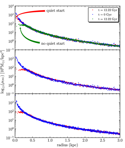
Figure 1: The density profile of the N03 NFW halo for different simulations: in the upper panel only DM was included, in the central panel DM, gas is included but star formation was turned off. The bottom panel shows the results of a simulation with DM, gas and star formation.

First, to test the stability of the NFW halos, we ran several simulations for the N03 and N05 mass models:

Run 1:

only DM

Run 2:

DM and gas but no star formation

Run 3:

DM and gas and star formation

For these test simulations an $n_{\rm SF}$ of $0.1\ \rm cm^{-3}$ (Katz et al., 1996) and $\epsilon_{\rm FB}$ of $0.1$ (Thornton et al., 1998) was used.

Fig. 1 shows the density profile of the test simulations for the N03 mass model. From the upper panel, it is evident that the DM density of the DM-only simulation remains stable and cusped until the end of the simulation. The simulations presented in the middle and bottom panels, show a clear conversion of the cusp into a core over time. Moreover, the width of the core depends on the mass of the system, with more massive halos having larger cores.

Our simulations largely confirm the results from Read & Gilmore (2005), where a rapid removal of gas results in a conversion from cusp to core as stated first by Navarro et al. (1996). As gas cools and flows into the halo, the center of the dark matter halo is adiabatically compressed. Without star formation, the central gas pressure builds up, eventually stops further inflow, and even makes the gas re-expand somewhat. This re-expansion happens rapidly enough for the DM halo to respond non-adiabatically: the central DM density experiences a net lowering and the cusp is transformed into a core. With star formation turned on, feedback is responsible for a fast removal of gas from the central parts of the DM halo, with the same effect: a conversion from a cusp to a core.

Unlike us, Governato et al. (2010) found that the density threshold for star formation needed to be high enough for a cusp-to-core conversion to occur. Only for $n_{\rm SF}\gtrsim 10$ cm^-3 does supernova feedback lead to sufficient gas motions to flatten the cusp in their simulated dwarfs, which are taken from a larger cosmological simulation. In contrast, in our more idealized, initially spherically symmetric setup, even a low density threshold leads to sufficient gas outflow for the cusp to flatten.

3.2 Star formation histories

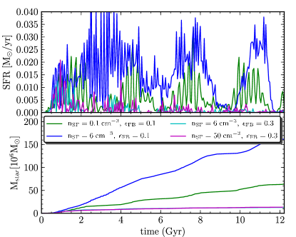
Figure 2: Top panel: the SFR of several N07 models as a function of time. Bottom panel: the stellar mass as a function of time.

In Fig. 2, we show the star-formation histories (SFHs) of different realizations of the N07 mass model. Also, in table 2, the starting time of star formation is tabulated along with the final total stellar mass. Several conclusions can be drawn:

• The delay between the start of the simulation and the start of the first star-formation event is an increasing function of $n_{\rm SF}$. This appears logical: it takes longer for the gas to collapse to higher densities and ignite star formation. Comparing different mass models, star formation starts earlier in more massive models for a given $n_{\rm SF}$. This is most likely due to the more massive models having steeper gravitational potential wells, increasing their ability to compress the inflowing gas.

• If $n_{\rm SF}$ is increased while $\epsilon_{\rm FB}$ is kept fixed, more stars are formed (e.g. going from the green to the blue curve or similarly from the cyan to the magenta curve in Fig. 2). This is because gas collapses to higher densities and the feedback is no longer able to sufficiently heat and expel this gas and to interrupt star formation.

• Related to the previous point, the SFR also becomes more rapidly varying if $n_{\rm SF}$ is increased while $\epsilon_{\rm FB}$ is kept fixed. The reason is that in the small high-density star-forming regions, feedback can only locally interrupt star formation during short timespans. At lower $n_{\rm SF}$, star formation is more widespread, leading to more global behavior: as supernovae go off, star formation can be completely halted.

• Increasing $\epsilon_{\rm FB}$ while $n_{\rm SF}$ is kept fixed leads to a decrease in star formation (e.g. going from the blue to the cyan curve in Fig. 2). This is because once feedback is strong enough, it is able to extinguish star formation, even at high gas densities.

• The most low-mass models fail to form stars for high $n_{\rm SF}$ values. E.g. no stars form in the N03 models for $n_{\rm SF}>0.1$ cm^-3. This is due to the masses of these models being too small for gas to collapse to densities where stars can be formed. This point is further elaborated in the next paragraph.

3.3 Density distribution of the ISM

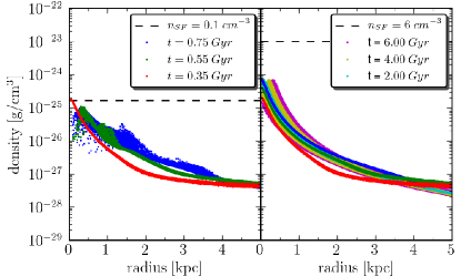
Figure 3: The density distribution of the ISM at different times for the least massive galaxy, N03, with different density threshold and a fixed feedback efficiency of 0.1.

In Fig. 3, the density of the ISM is plotted as a function of radius. For the N03 model in the left panel a density threshold of $0.1$ cm^-3 was used while for the model in the right panel, the density threshold was set to a value of $6$ cm^-3. The red points show the gas distribution at the moment just before the start of star formation in the case of $n_{\rm SF}$ = $0.1$ cm^-3. Since up to that moment, all models have experienced the same evolution, there is no difference between the red points in both panels. As can be seen in the left panel, the gas density in this N03 model reaches the star-formation threshold and star formation occurs. Moreover, the influence of supernova feedback can be seen in the green and blue points, where gas expands to larger radii and lower densities after having been heated. As is clear from the right panel, for $n_{\rm SF}$ = $6$ cm^-3 the gas simply keeps falling in. It will continue to do so during the first 4 Gyr until the built-up central pressure causes the gas to re-expand again. No stars are formed during the course of this simulation.

As the density threshold is increased to higher values, star formation tends to occur more and more in small collapsed clumps. This becomes clear when comparing the panels from Figs. 3 and 4. The latter shows the gas density distributions of two N07 models with $n_{\rm SF}$ = $6$ cm^-3 and $n_{\rm SF}$ = $50$ cm^-3. While the $n_{\rm SF}$ = $50$ cm^-3 model only exhibits star formation in a small number of discrete high-density clumps, the $n_{\rm SF}$ = $6$ cm^-3 model lacks such well-defined clumps and star formation occurs more widespread.

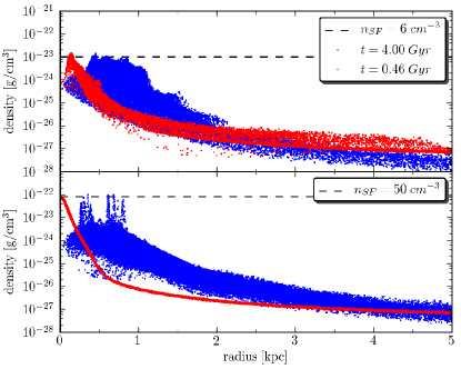
Figure 4: The density distribution of the ISM at different times for the N07 model, with different density thresholds and a fixed feedback efficiency of 0.7.

3.4 Scaling relations

In this section we discuss the properties of each of our models and draw some conclusions regarding the influence of the $n_{\rm SF}$ and $\epsilon_{\rm FB}$ parameters on the models. An overview of some basic properties can be found in Table 2.

Table 2: Final properties of our large set of simulations. Columns: (1) model number (see Table 1), (2) density treshold for star formation, (3) feedback efficiency, (4) final stellar mass, (5) starting time of star formation, (6) half-light radius, (7) mean surface brightness within the half-light radius, (8) central one dimensional velocity dispersion, (9) mass-weighted metallicity, (10) central surface brightness, (11) Sérsic parameter, (12) circular velocity.

$\mathrm{Model}$	$\mathrm{n_{\rm SF}}$	$\epsilon_{\rm FB}$	$M_{\rm\star,f}$	$\Delta T_{\rm SF}$	$R_{\rm e}$	$I_{\rm e}$	$\sigma_{\rm 1D,c}$	$V-I$	$[Fe/H]$	$\mu_{0}$	$n$	$V_{\rm c}$
	$[cm^{-3}]$		$[10^{6}\ M_{\odot}]$	$[Gyr]$	$[kpc]$		$[km/s]$			$[mag]$		$[km/s]$
N03	0.1	0.1	0.285	0.342	0.100	3.176	6.806	0.835	-1.183	23.603	1.496	16.176
N05	0.1	0.1	5.667	0.168	0.230	10.779	12.190	0.860	-1.236	23.170	0.959	20.396
[1pt/5pt] N05	6	0.1	17.867	0.546	0.130	88.566	12.253	0.910	-0.659	20.920	1.025	22.574
N05	6	0.3	4.049	0.546	0.142	18.222	9.131	0.870	-1.130	23.005	0.877	20.483
N05	6	0.5	2.021	0.546	0.134	11.813	8.310	0.839	-1.302	22.586	1.137	20.590
N05	6	0.7	1.174	0.546	0.118	9.252	8.107	0.817	-1.542	22.694	1.231	20.555
N05	6	0.9	1.017	0.546	0.122	7.070	8.195	0.831	-1.552	24.139	0.785	20.096
[1pt/5pt] N05	50	0.3	6.116	0.688	0.244	10.945	8.346	0.852	-1.016	23.154	1.104	21.158
N05	50	0.5	3.230	0.688	0.152	11.699	8.116	0.878	-1.242	22.952	1.117	20.342
N05	50	0.7	2.128	0.688	0.141	10.182	8.362	0.829	-1.426	23.141	1.112	20.038
N05	50	0.9	1.625	0.688	0.157	5.196	8.423	0.864	-1.461	24.313	0.928	19.563
N06	0.1	0.1	15.616	0.137	0.384	11.813	16.209	0.856	-1.108	23.730	0.718	23.290
[1pt/5pt] N06	6	0.1	42.542	0.460	0.150	198.791	16.779	0.870	-0.540	20.383	0.892	27.277
N06	6	0.3	5.154	0.460	0.149	22.155	9.430	0.845	-1.289	22.362	1.005	21.828
N06	6	0.5	3.425	0.460	0.156	16.053	8.875	0.832	-1.329	22.981	0.872	21.335
N06	6	0.7	2.030	0.460	0.136	11.336	8.956	0.823	-1.459	23.181	0.993	21.764
N06	6	0.9	2.255	0.460	0.161	9.701	8.640	0.830	-1.437	23.493	0.935	21.668
[1pt/5pt] N06	50	0.3	10.227	0.591	0.256	15.982	9.629	0.856	-1.054	23.001	0.905	23.250
N06	50	0.5	5.780	0.591	0.173	16.660	9.040	0.866	-1.228	22.497	1.142	21.697
N06	50	0.7	3.306	0.591	0.187	8.347	9.634	0.843	-1.392	23.103	1.228	21.332
N06	50	0.9	2.718	0.591	0.180	7.722	9.041	0.838	-1.408	23.093	1.228	21.089
N07	0.1	0.1	67.575	0.135	0.693	14.994	23.992	0.887	-0.808	23.281	0.889	30.289
[1pt/5pt] N07	6	0.1	161.970	0.336	0.206	326.861	28.621	0.900	-0.361	19.621	0.910	39.206
N07	6	0.3	14.933	0.336	0.220	31.447	10.274	0.843	-1.133	21.839	1.076	23.908
N07	6	0.5	8.008	0.336	0.190	20.299	10.485	0.825	-1.415	22.718	0.899	23.673
N07	6	0.7	5.046	0.336	0.192	13.261	9.642	0.816	-1.480	22.874	1.054	23.759
N07	6	0.9	4.246	0.336	0.193	9.060	10.028	0.853	-1.562	23.629	0.977	23.004
[1pt/5pt] N07	50	0.3	21.037	0.460	0.322	18.593	9.452	0.870	-1.056	22.234	1.146	24.773
N07	50	0.5	14.128	0.460	0.340	11.805	10.721	0.864	-1.168	23.296	0.965	24.948
N07	50	0.7	9.027	0.460	0.477	3.644	10.586	0.862	-1.294	24.391	1.066	24.018
N07	50	0.9	4.908	0.460	0.396	3.605	8.229	0.819	-1.415	24.532	0.972	24.537
N08	0.1	0.1	155.430	0.131	0.812	25.902	29.448	0.871	-0.665	22.506	0.966	35.875
[1pt/5pt] N08	6	0.1	271.070	0.278	0.163	839.934	-99.000	0.893	-0.261	17.300	1.467	43.269
N08	6	0.3	24.623	0.278	0.253	34.853	12.685	0.864	-1.019	21.662	1.111	27.178
N08	6	0.5	12.423	0.278	0.248	17.704	12.089	0.838	-1.404	22.986	0.846	25.561
N08	6	0.7	9.402	0.278	0.229	14.476	11.430	0.842	-1.534	22.917	1.003	24.198
N08	6	0.9	0.610	0.278	0.086	128.570	8.947	0.454	-4.277	20.621	1.077	27.395
[1pt/5pt] N08	50	0.3	42.956	0.392	0.362	26.137	11.375	0.900	-0.931	21.234	1.542	27.570
N08	50	0.5	22.743	0.393	0.481	9.039	11.535	0.860	-1.147	23.855	0.768	27.479
N08	50	0.7	15.763	0.393	0.437	9.845	11.364	0.819	-1.186	23.771	0.737	28.530
N08	50	0.9	9.019	0.393	0.400	5.897	12.584	0.842	-1.331	24.193	0.836	27.050
N09	0.1	0.1	394.500	0.104	0.616	109.262	38.883	0.841	-0.382	20.759	0.943	48.060
[1pt/5pt] N09	6	0.1	477.620	0.235	0.224	385.748	-99.000	1.051	-0.215	18.931	1.351	57.020
N09	6	0.3	86.095	0.235	0.278	82.718	18.482	0.898	-0.911	20.249	1.388	31.210
N09	6	0.5	30.470	0.235	0.324	21.627	13.867	0.874	-1.282	22.310	1.132	29.103
N09	6	0.7	19.274	0.235	0.500	6.815	11.576	0.843	-1.356	23.629	0.969	29.240
N09	6	0.9	12.881	0.235	0.318	9.233	12.614	0.853	-1.640	23.104	1.236	28.515
[1pt/5pt] N09	50	0.3	94.102	0.324	0.382	45.638	14.780	0.901	-0.917	20.402	1.541	31.697
N09	50	0.5	40.965	0.324	0.409	17.192	14.266	0.883	-1.218	22.887	0.930	29.369
N09	50	0.7	23.972	0.324	0.559	5.967	13.400	0.867	-1.330	23.974	1.037	29.311
N09	50	0.9	15.385	0.324	0.503	6.225	12.743	0.830	-1.396	24.465	0.691	30.326

3.4.1 Half-light radius $R_{e}$

The half-light radius, or effective radius, denoted by $R_{e}$, encloses half of a galaxy’s luminosity. In panel a.) of Fig. 5, $R_{e}$ is plotted as a function of the $V$-band magnitude. The following trends can be observed in this figure:

• For a fixed $n_{\rm SF}$, the effective radius varies only very slightly throughout the $\epsilon_{\rm FB}$-range and this without a clear trend between $R_{e}$ and $\epsilon_{\rm FB}$. However, for a fixed $n_{\rm SF}$ and dark-matter mass the stellar mass and consequently the luminosity decrease with increasing $\epsilon_{\rm FB}$. This is due to star formation being shut down more rapidly when feedback is more effective. As a result, galaxies tend to have higher stellar densities for smaller $\epsilon_{\rm FB}$.

• For a fixed $\epsilon_{\rm FB}$ of 0.1, an increase of $n_{\rm SF}$ from $0.1$ to $6$ cm^-3 results in a decrease of the effective radius. This is due to the size of the region where the SFC are fulfilled, which is much smaller for $n_{\rm SF}$ = $6$ cm^-3 than for $n_{\rm SF}$ = $0.1$ cm^-3, and the feedback is too weak to overcome this. In the case of an increase of $n_{\rm SF}$ from $6$ to $50$ cm^-3, the effective radius increases which is caused by the higher star formation peaks resulting in more supernovae explosions which redistribute the gas more efficiently.

• The simulations with high density threshold, $n_{\rm SF}>0.1\ \rm cm^{-3}$, and high feedback efficiency, $\epsilon_{\rm FB}>0.1$, have effective radii which are in agreement with the observations.

From this scaling relation we can constrain the $\epsilon_{\rm FB}$-parameter to be higher then 0.1 to produce galaxies with effective radii in agreement with observations of dwarf galaxies.

3.4.2 The fundamental plane

The fundamental plane (FP) is an observed relation between the effective radius, $R_{\rm e}$, the mean surface brightness within the effective radius, $I_{\rm e}$, and the central velocity dispersion, $\sigma_{\rm c}$ of giant elliptical galaxies. It is a linear relation, given by

$$\log(R_{\rm e})=-0.629-0.845\log(I_{\rm e})+1.38\log(\sigma_{\rm c}),$$ (10)

between the logarithms of these quantities (Burstein et al., 1997). In panel b.) of Fig. 5, we plot the ”vertical” deviation of the simulated galaxies from the giant galaxies’ FP.

Dwarf galaxies generally lie above the FP in this projection. This is thought to be a consequence of their having shallower gravitational potential wells than giant galaxies. This, together with the feedback, results in more diffuse systems. Models with a high star-formation threshold in combination with a low supernova feedback turn out to be very compact. They actually populate the FP at low luminosities. However, this region of the three-dimensional space spanned by $\log(R_{\rm e})$, $\log(I_{\rm e})$, and $\log(\sigma_{\rm c})$ is observed to be devoid of galaxies. Hence, models with low stellar feedback, $\epsilon_{\rm FB}$ up to $0.3$, and high density thresholds, $n_{\rm SF}>0.1$ cm^-3, can be rejected.

Figure 5: Some scaling relations and the surface brightness parameters as a function of the magnitude. In a.), the half-light radius $R_{\rm e}$ is plotted, b.) shows the vertical deviation of the simulated dwarf galaxies from the giant galaxies’ FP, in c.) the $V-I$ color is plotted, d.) shows the iron content $[Fe/H]$. In panel e.) and f.), the Sérsic index $n$ and central surface brightness $\mu_{0}$ are plotted. All these quantities are plotted against the $V$-band magnitude, except the FP which are plotted as a function of the $B$-band luminosity. The models with a density threshold of $6\rm~{}cm^{-3}$ and $50\rm~{}cm^{-3}$ are represented by blue-green diamonds and yellow-red triangles, respectively, where the colorscales represent a varying feedback efficiency. For each color, the datapoints are connected by a line showing the mass evolution of the models. In the case of $n_{\rm SF}=0.1\ cm^{-3}$, represented by the black line, the models from N03 until N09 are plotted. In the cases of higher densities, represented by the colored lines, the datapoints are from models N05-N09. Our models are compared with observational data obtained from De Rijcke et al. (2005), Graham et al. (2003) , LG data come from Peletier & Christodoulou (1993), Peletier & Christodoulou (1993), Irwin & Hatzidimitriou (1995), Saviane et al. (1996), Grebel et al. (2003), McConnachie & Irwin (2006), McConnachie et al. (2007), Zucker et al. (2007), Perseus data from De Rijcke et al. (2009), Antlia data from Smith Castelli et al. (2008). For the $[Fe/H]-M_{V}$ plot, data from Grebel et al. (2003), Sharina et al. (2008) and Lianou et al. (2010) was used, the yellow and magenta dots represent data from dSph and dIrr galaxies, respectively.

3.4.3 Color $V-I$

Fig. 5, panel c.) shows the $V-I$ color in function of the $V$-band magnitude. The color scatter between the different models is rather small. The observed galaxies follow a mass-metallicity relation so the metallicity generally increases with the galaxy (stellar) mass, resulting in increasing $V-I$ values for increased galaxy mass. Within the relatively small mass range covered by the models, color is only a very weak function of stellar mass. For a fixed feedback efficiency, when increasing the density threshold the $V-I$ also increases slightly resulting in bluer galaxies for the models with low density threshold. This is due to the effect that stars are formed in more metal enriched regions in the models with high density threshold. When the density threshold is kept constant and only the feedback efficiency is increased the $V-I$ slightly decreases, so the models get slightly bluer due to a dilution of the gas when it is more spread out by supernovae explosions.

3.4.4 Metallicity

In panel d.) of Fig. 5 a plot of iron content [Fe/H] as a function of the $V$-band magnitude is shown. The mass-weighted value of [Fe/H] is a measure of the metallicity of a galaxy. The yellow and magenta dots represent observational data from dwarf spheroidal and dwarf elliptical galaxies and irregular dwarf galaxies, respectively. Some general conclusions we can take away from this figure are:

• Low-mass models with low density threshold, $n_{\rm SF}\approx 0.1$ cm^-3, and low feedback, $\epsilon_{\rm FB}\approx 0.1$, keep forming stars throughout cosmic history and do not expel enriched gas. As a consequence, they turn out to be too metal rich, compared with observed dwarf galaxies. Models with higher $n_{\rm SF}$ compare much more favorably with the data in this respect.

• For a fixed $n_{\rm SF}$, increasing $\epsilon_{\rm FB}$, produces more metal poor galaxies. This is likely due to the fact that the increased feedback extinguishes star formation more rapidly and disperses the metal enriched gas more widely.

• Increasing $n_{\rm SF}$ at fixed $\epsilon_{\rm FB}$ and fixed mass, results in an increase of the metallicity and of the stellar mass when going from $n_{\rm SF}=0.1$ cm^-3 to $n_{\rm SF}=6$ cm^-3. A further increase of $n_{\rm SF}$ at fixed $\epsilon_{\rm FB}$, up to $n_{\rm SF}=50$ cm^-3, has a much smaller impact on metallicity and stellar mass. The former is likely due to more vigorous star formation in less easily dispersable high density regions.

3.4.5 Surface brightness profiles

We fitted a Sérsic profile, of the form

$$I(R)=I_{0}e^{-\left(\frac{R}{R_{0}}\right)^{1/n}},$$ (11)

to the surface brightness profiles of the simulated galaxies. The Sérsic parameter $n$ and the central surface brightness $\mu_{0}$ are plotted respectively in the panels e.) and f.) of Fig. 5 as a function of the $V$-band magnitude.

• For a fixed $n_{\rm SF}$, when increasing the $\epsilon_{\rm FB}$, there is a weak trend for the Sérsic parameter $n$ and the central surface brightness to decrease. More vigorous feedback appears to result in more diffuse dwarf galaxies, as one would expect.

• As an echo of the $R_{\rm e}-M_{\rm V}$ relation, simulations with high density threshold, $n_{\rm SF}>0.1\ \rm cm^{-3}$, and low feedback efficiency, $\epsilon_{\rm FB}=0.1-0.3$, are systematically too compact, with $\mu_{0}\sim 20$ mag arcsec^-2, compared with the observations.

• The models with high density thresholds and strong feedback are in general agreement with the observations.

3.4.6 The Tully-Fisher relation

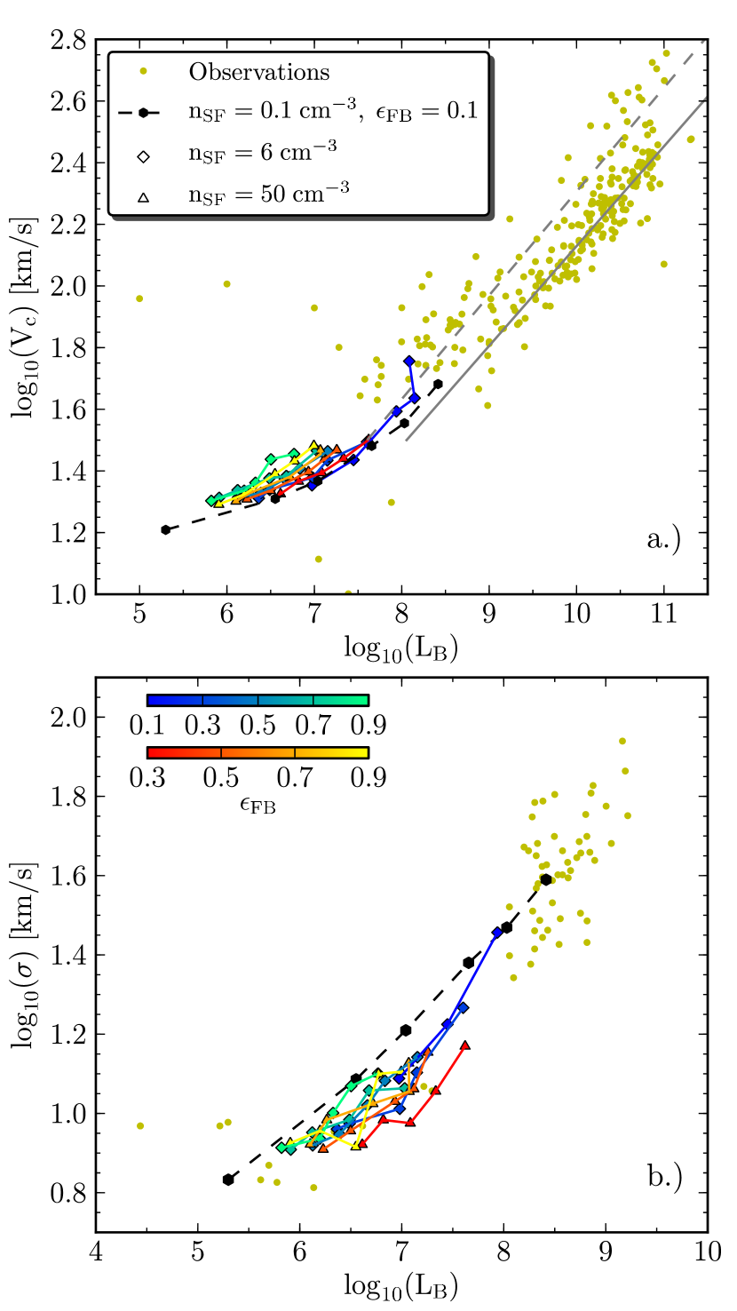
Figure 6: The top panel shows the Tully-Fisher relation between the circular velocity and the luminosity in the B-band. The full gray line shows the TF relation for early type galaxies, the dashed gray line is the TF relation of spiral galaxies as determined by De Rijcke et al. (2007). The lower panel shows the Faber-Jackson relation between the velocity dispersion and the luminosity in the B-band.

Panel a.) of Fig. 6 shows the B-band Tully-Fisher relation (TFR) between the circular velocity, denoted by $V_{c}$, and the luminosity in the B-band, $L_{\rm B}$. The simulations are compared with observational data and with the Tully-Fisher relation for early-type (full gray line) and for spiral galaxies (dotted gray line) that was determined by De Rijcke et al. (2007). All simulations predict that the TFR becomes substantially shallower in the dwarf regime, below luminosities of the order of $L_{\rm B}\sim 10^{7}\,L_{\odot,\rm B}$. This can be seen as a consequence of the very steep $M_{\rm star}-M_{\rm halo}$ relation in the dwarf galaxy regime (see paragraph 3.4.8). For a fixed $n_{\rm SF}$, an increase in feedback efficiency does not influence $V_{c}$ very much since there are so few stars that $V_{c}$ is set by the dark-matter halo. The effect on the stellar mass, and consequently on $L_{\rm B}$, is, however, quite large. Therefore, increasing $\epsilon_{\rm FB}$ at fixed $n_{\rm SF}$ and dark-matter mass causes galaxies to shift leftwards in panel a.) of Fig. 6. Except for this effect, once $n_{\rm SF}$ and $\epsilon_{\rm FB}$ are raised above their minimum values of $0.1$ cm^-3 and $0.1$, respectively, there is no significant differences between the TFRs traced by the different series of models.

3.4.7 The Faber-Jackson relation

The Faber-Jackson (FJR) relation, plotted in panel b.) of Fig. 6 is the relation between the stellar central velocity dispersion and the luminosity in the $B$-band. The stellar central velocity dispersion is a projection of the velocity dispersion along the line of sight. This is measured by fitting an exponential function to the dispersion profile and retaining the maximum of the function as the central value.

From this figure we see:

• For a fixed $n_{\rm SF}$, when increasing the $\epsilon_{\rm FB}$, the velocity dispersion decreases first after which it settles around a value which depends on the dark-matter mass of the model.

• For a fixed $\epsilon_{\rm FB}$, when increasing $n_{\rm SF}$, only a minor influence on the velocity dispersion is observed.

3.4.8 The $M_{\rm star}$-$M_{\rm halo}$ relation

In Fig. 7, the $M_{\rm star}$-$M_{\rm halo}$ relation of the simulations at $z=0$ is plotted. We can make similar conclusions here as were made in the SFH section:

• If $n_{\rm SF}$ is fixed, the stellar mass will decrease if the $\epsilon_{\rm FB}$ is increased. This is what was expected because with more feedback the gas is distributed over a larger area and the infall of the gas to the appropriate density threshold will take longer.

• If $\epsilon_{\rm FB}$ is fixed, for increasing $n_{\rm SF}$, the stellar mass increases too. When feedback is very small, the gas density will stay high and the star formation will not be interrupted, resulting in a high stellar mass. The effect is smaller for higher feedback.

In Fig. 7, our different sets of models are found to be in agreement with the results from the Aquila simulation where a density threshold of 10 $\rm cm^{-3}$ and a feedback efficiency of 0.7 was used. While the initial conditions of our dwarf galaxy simulations are admittedly quite simplified, they do have high spatial resolution and realistic implemented physics. It is therefore encouraging that they compare favorably with cosmological simulations like the Aquila simulation, which have cosmologically well motivated initial conditions but in which dwarf galaxies are very close to the resolution limit (Sawala et al., 2011). However it is impossible by further tuning of the feedback efficiency and/or the density threshold to reproduce the trend that was derived by Guo et al. (2010).

By increasing the density threshold and feedback efficiency, the stellar mass is reduced by almost two orders of magnitude, but there still remains a difference of many orders of magnitude between our simulations and the $M_{\star}$-$M_{halo}$ relation from Guo et al. (2010). It is also interesting to notice that although our models do not reproduce the relation, they do have a very similar slope.

4 Discussion and conclusions

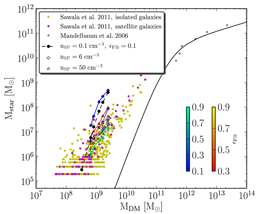
Figure 7: The stellar mass versus the DM halo mass, plotted in comparison with the models by Sawala et al. (2011). The gray dots show data from gravitational lensing from Mandelbaum et al. (2006). The black line is the trend for this relation that was determined by Guo et al. (2010).

4.1 Cusp to core

Whether the halo density profile is cusped or cored has been a point of discussion for quite some time. Observationally, evidence for cored DM profiles is found (Gentile et al., 2004), but from cosmological DM simulations a cusped density profile is deduced (Navarro et al., 1996; Moore et al., 1996). The inherent limitation due to the angular resolution of the observations is ruled as a cause of the observed flat density profiles by de Blok & Bosma (2002). Gentile et al. (2005) also excluded the possibility of non-circular gas motions which might result in a rotation curve that is best fitted by a cored halo, while the dark matter halo actually has a cuspy profile. However, from the simulation point of view, Mashchenko et al. (2006) mentioned a natural transition of a cusp to a flattened core when the dark matter halo is gravitationally heated by bulk gas motions.

Our simulations are set up with a cusped NFW halo in agreement with cosmological simulations. The infall of gas causes an adiabatic compression of the dark halo. When gas is evacuated from the central regions, be it by a fast re-expansion as the gas pressure builds up or by supernova feedback, the dark-matter halo reacts non-adiabatically and kinetic energy of the gas is transferred to the dark matter. This results in a flattening of the central density and so the cusp is converted into a core. We can conclude that the conversion of the cusped halo density profile to a cored profile is realized by the removal of baryons from the galaxy center (Read & Gilmore, 2005), whether this is due to a re-expansion of the gas or by feedback effects or by another process.

4.2 Degeneracy

By increasing both the density threshold and the feedback efficiency, the simulated galaxies move along the observed kinematic and photometric scaling relations. These two parameters, the feedback efficiency $\epsilon_{\rm FB}$ and the density threshold $n_{\rm SF}$, correlate with each other and an increase of the one can be counteracted by an increase of the other, resulting in galaxies with similar properties. To be more specific: the individual galaxies are drastically different for different parameter values but they all line up along the same scaling relations and can therefore be seen as good analogs of observed dwarf galaxies.

The feedback efficiency quantifies the fraction of the $10^{51}$ ergs of energy that are released during a supernova explosion and thermally injected into the ISM. For each value of the density threshold we can determine the feedback efficiency range for which the models are in agreement with the observations, although we are not able to deduce a unique $n_{\rm SF}$/$\epsilon_{\rm FB}$-combination which would be the “correct“ representation of the physical processes that happen in galaxies.

For a certain density threshold, a lower limit of the corresponding $\epsilon_{\rm FB}$-parameter can be determined from the effective radius: the galaxies become too centrally concentrated when the feedback is too low. From the scaling relations we cannot deduce an upper limit for the $\epsilon_{\rm FB}$-parameter, but one could argue that the ISM cannot receive more energy than there is released by the supernova explosion, resulting in a maximal value for the feedback efficiency of 1.

In the case of a density threshold of $n_{\rm SF}=0.1$ cm^-3, the models are generally in good agreement with the observations besides the somewhat high metallicities. This is also the reason why the feedback efficiency was not varied in this case. If we compare the high density threshold models, $n_{\rm SF}>0.1$ cm^-3, with the observations we can conclude that the feedback efficiency should be larger then $\sim 0.3$. For a density threshold of $n_{\rm SF}=6$ cm^-3, we prefer a value of 0.7 for the feedback. Similarly we prefer a feedback efficiency of 0.9 in the case of a density threshold of $n_{\rm SF}=50$ cm^-3

The fact that different $n_{\rm SF}$/$\epsilon_{\rm FB}$-combinations result in simulated galaxies with properties that are in agreement with the observations invokes a warning for future simulations and indicates that there is still some work left to determine the density of the star forming regions and the fraction of supernova energy that is absorbed by the ISM, quantities which are hard to determine observationally.

There are however other parameters that might influence the starformation rate and our degeneracy, which are not investigated here:

• Given the fact that the star-formation efficiency $c_{\star}$ was found by other authors not to have a significant impact on stellar mass, we did not investigate it in detail in this paper.

• The choice of the IMF, for which in our simulations a Salpeter IMF is used, determines the mass distribution of stars. The fraction of high-mass stars influences the number of SNIa and SNII explosions and as a consequence it will influence the amount of feedback and the chemical evolution. However, given the large number of IMF parameterizations available in the literature, testing them is a very daunting task which falls outside the scope of this paper. Moreover, part of the IMF-variation is quantified approximately by the variation in $\epsilon_{\rm FB}$ which we do investigate.

• There are other possible feedback implementations, next to the release of feedback energy as thermal energy to the gas. It also could be released as kinetic energy by kicking the gas particles or by blast-wave feedback (Mayer et al., 2008).

• Other implementations of star formation, e.g. based on a subgrid model of H₂-formation (Pelupessy et al., 2004), are possible.

  4.3 The dwarf galaxy dark-matter halo occupancy

  To conclude, Fig. 8 shows the models which best agree with the observations for each density threshold that was used in our analysis. Increasing $n_{\rm SF}$ together with $\epsilon_{\rm FB}$ leads to a strong reduction, of almost two orders of magnitude, of the stellar mass, especially in the most massive models. However, with the physics included in our simulations, we are unable to reproduce the $M_{\rm star}-M_{\rm halo}$ relation of Guo et al. (2010). Surprisingly, the best models trace a $M_{\rm star}-M_{\rm halo}$ relation with a slope that is similar to that of the relation of Guo et al. (2010). Our simulations are in agreement with results from cosmological simulations, which have, however, much lower spatial resolution in the dwarf regime Sawala et al. (2011). We did not explore yet higher values for $n_{\rm SF}$ and $\epsilon_{\rm FB}$ because it is clear from Fig. 8 that the reduction of $M_{\rm star}$ stagnates for high $n_{\rm SF}$-values. Moreover, to compensate for the high density threshold, an unphysical large value for $\epsilon_{\rm FB}$, higher than 1, would be required. Thus, we arrive at $(n_{\rm SF}=6\,{\rm cm}^{-3},\,\epsilon_{\rm FB}\sim 0.7)$ and $(n_{\rm SF}=50\,{\rm cm}^{-3},\,\epsilon_{\rm FB}\sim 0.9)$ as the models which are in best agreement with the observed photometric and kinematical scaling relations and with the $M_{\rm star}-M_{\rm halo}$ relation derived directly from cosmological simulations.

  

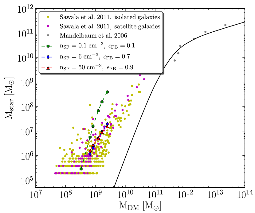
  Figure 8: The $M_{\rm star}-M_{\rm halo}$ of our best models for different density threshold compared to the relation of Guo et al. 2010, other simulations from Sawala et al. 2011 and observations from Mandelbaum et al. 2006.

  While it appears impossible to place isolated dwarf galaxies on the $M_{\rm star}-M_{\rm halo}$ relation of Guo et al. (2010), it is possible to envisage external influences that may further reduce $M_{\rm star}$, as already mentioned in the Introduction:

  • Not properly taking into account the effects of reionisation may lead to an overestimation of the gas content of dwarfs and an underestimation of the gas cooling time. However, even taking into account reionisation, the dwarf galaxies simulated by Sawala et al. (2011) had much too high stellar masses.

  • At a given gas density, the star-formation efficiency of dwarf galaxies could be lower than that of more massive stellar systems because of their lower metallicity and hence lower dust content. This could be mimicked by reducing the star-formation efficiency parameter $c_{\star}$ (see eq. (8)) in the dwarf regime. However, Stinson et al. (2006) have shown that, because of self-regulation, the star-formation rate is very insensitive to this parameter: varying $c_{\star}$ between 0.05 and 1 left the mean star-formation rate virtually unchanged.

  • External processes such as ram-pressure stripping and tidal stirring may lead to a premature cessation of star formation and hence lower $M_{\rm star}$ (Mayer et al., 2006). However, these processes are only effective if the gravitational potential wells of dwarf galaxies are sufficiently shallow and if they are stripped early enough in cosmic history, before they converted their gas into stars. It is unclear whether these constraints are met. In De Rijcke et al. (2010), and references therein, it was argued that the number of red-sequence, quenched dwarf galaxies increased significantly over the last half of the Hubble time and that the dwarf galaxies now residing in the Fornax cluster were accreted less than a few crossing times age (i.e. less than a few Gyr). This timescale would have left dwarf galaxies ample time to form stars before entering the cluster.

  Acknowledgements

  We thank Volker Springel for making publicly available the Gadget-2 simulation code and Till Sawala for making available to us his data from the Aquila simulation. We also would like to thank the anonymous referee for his/her stimulating remarks that have greatly improved the manuscript.

References

- Barnabè et al. (2009) Barnabè M., Czoske O., Koopmans L. V. E., Treu T., Bolton A. S., Gavazzi R., 2009, MNRAS, 399, 21
- Burstein et al. (1997) Burstein D., Bender R., Faber S., Nolthenius R., 1997, ApJ, 114, 1365
- Buyle et al. (2006) Buyle P., Michielsen D., de Rijcke S., Ott J., Dejonghe H., 2006, MNRAS, 373, 793
- Buyle et al. (2007) Buyle P., van Hese E., de Rijcke S., Dejonghe H., 2007, MNRAS, 375, 1157
- de Blok & Bosma (2002) de Blok W. J. G., Bosma A., 2002, A&A, 385, 816
- De Rijcke et al. (2005) De Rijcke S., Michielsen D., Dejonghe H., Zeilinger W. W., Hau G. K. T., 2005, A&A, 438, 491
- De Rijcke et al. (2009) De Rijcke S., Penny S. J., Conselice C. J., Valcke S., Held E. V., 2009, MNRAS, 393, 798
- De Rijcke et al. (2006) De Rijcke S., Prugniel P., Simien F., Dejonghe H., 2006, MNRAS, 369, 1321
- De Rijcke et al. (2010) De Rijcke S., Van Hese E., Buyle P., 2010, ApJL, 724, L171
- De Rijcke et al. (2007) De Rijcke S., Zeilinger W. W., Hau G. K. T., Prugniel P., Dejonghe H., 2007, ApJ, 659, 1172
- Gentile et al. (2005) Gentile G., Burkert A., Salucci P., Klein U., Walter F., 2005, ApJL, 634, L145
- Gentile et al. (2004) Gentile G., Salucci P., Klein U., Vergani D., Kalberla P., 2004, MNRAS, 351, 903
- Gnedin et al. (2009) Gnedin N. Y., Tassis K., Kravtsov A. V., 2009, ApJ, 697, 55
- Governato et al. (2010) Governato F., Brook C., Mayer L., Brooks A., Rhee G., Wadsley J., Jonsson P., Willman B., Stinson G., Quinn T., Madau P., 2010, Nature, 463, 203
- Graham et al. (2003) Graham A. W., Jerjen H., Guzmán R., 2003, ApJ, 126, 1787
- Grebel et al. (2003) Grebel E. K., Gallagher III J. S., Harbeck D., 2003, ApJ, 125, 1926
- Guo et al. (2010) Guo Q., White S., Li C., Boylan-Kolchin M., 2010, MNRAS, 404, 1111
- Irwin & Hatzidimitriou (1995) Irwin M., Hatzidimitriou D., 1995, MNRAS, 277, 1354
- Katz et al. (1996) Katz N., Weinberg D. H., Hernquist L., 1996, ApJs, 105, 19
- Kronawitter et al. (2000) Kronawitter A., Saglia R. P., Gerhard O., Bender R., 2000, A&AS, 144, 53
- Lianou et al. (2010) Lianou S., Grebel E. K., Koch A., 2010, A&A, 521, A43
- Liesenborgs et al. (2009) Liesenborgs J., de Rijcke S., Dejonghe H., Bekaert P., 2009, MNRAS, 397, 341
- Maio et al. (2007) Maio U., Dolag K., Ciardi B., Tornatore L., 2007, MNRAS, 379, 963
- Mandelbaum et al. (2006) Mandelbaum R., Seljak U., Kauffmann G., Hirata C. M., Brinkmann J., 2006, MNRAS, 368, 715
- Mashchenko et al. (2006) Mashchenko S., Couchman H. M. P., Wadsley J., 2006, Nature, 442, 539
- Mashchenko et al. (2008) Mashchenko S., Wadsley J., Couchman H. M. P., 2008, Science, 319, 174
- Mayer et al. (2008) Mayer L., Governato F., Kaufmann T., 2008, Advanced Science Letters, 1, 7
- Mayer et al. (2006) Mayer L., Mastropietro C., Wadsley J., Stadel J., Moore B., 2006, MNRAS, 369, 1021
- McConnachie et al. (2007) McConnachie A. W., Arimoto N., Irwin M., 2007, MNRAS, 379, 379
- McConnachie & Irwin (2006) McConnachie A. W., Irwin M. J., 2006, MNRAS, 365, 1263
- Moore et al. (1996) Moore B., Katz N., Lake G., 1996, ApJ, 457, 455
- Napolitano et al. (2011) Napolitano N. R., Romanowsky A. J., Capaccioli M., Douglas N. G., Arnaboldi M., Coccato L., Gerhard O., Kuijken K., Merrifield M. R., Bamford S. P., Cortesi A., Das P., Freeman K. C., 2011, MNRAS, 411, 2035
- Navarro et al. (1996) Navarro J. F., Eke V. R., Frenk C. S., 1996, MNRAS, 283, L72
- Navarro et al. (1996) Navarro J. F., Frenk C. S., White S. D. M., 1996, ApJ, 462, 563
- Peletier & Christodoulou (1993) Peletier R. F., Christodoulou D. M., 1993, ApJ, 105, 1378
- Pelupessy et al. (2004) Pelupessy F. I., van der Werf P. P., Icke V., 2004, A&A, 422, 55
- Read & Gilmore (2005) Read J. I., Gilmore G., 2005, MNRAS, 356, 107
- Revaz et al. (2009) Revaz Y., Jablonka P., Sawala T., Hill V., Letarte B., Irwin M., Battaglia G., Helmi A., Shetrone M. D., Tolstoy E., Venn K. A., 2009, A&A, 501, 189
- Saviane et al. (1996) Saviane I., Held E. V., Piotto G., 1996, A&A, 315, 40
- Sawala et al. (2011) Sawala T., Guo Q., Scannapieco C., Jenkins A., White S., 2011, MNRAS, 413, 659
- Sawala et al. (2011) Sawala T., Scannapieco C., White S., 2011, ArXiv e-prints
- Schmidt (1959) Schmidt M., 1959, apj, 129, 243
- Schroyen et al. (2011) Schroyen J., De Rijcke S., Valcke S., Cloet-Osselaer A., Dejonghe H., 2011, ArXiv e-prints
- Sellwood & Athanassoula (1986) Sellwood J. A., Athanassoula E., 1986, MNRAS, 221, 195
- Sharina et al. (2008) Sharina M. E., Karachentsev I. D., Dolphin A. E., Karachentseva V. E., Tully R. B., Karataeva G. M., Makarov D. I., Makarova L. N., Sakai S., Shaya E. J., Nikolaev E. Y., Kuznetsov A. N., 2008, MNRAS, 384, 1544
- Smith Castelli et al. (2008) Smith Castelli A. V., Bassino L. P., Richtler T., Cellone S. A., Aruta C., Infante L., 2008, MNRAS, 386, 2311
- Springel (2005) Springel V., 2005, MNRAS, 364, 1105
- Stinson et al. (2006) Stinson G., Seth A., Katz N., Wadsley J., Governato F., Quinn T., 2006, MNRAS, 373, 1074
- Stinson et al. (2009) Stinson G. S., Dalcanton J. J., Quinn T., Gogarten S. M., Kaufmann T., Wadsley J., 2009, MNRAS, 395, 1455
- Stinson et al. (2007) Stinson G. S., Dalcanton J. J., Quinn T., Kaufmann T., Wadsley J., 2007, ApJ, 667, 170
- Sutherland & Dopita (1993) Sutherland R. S., Dopita M. A., 1993, ApJS, 88, 253
- Thornton et al. (1998) Thornton K., Gaudlitz M., Janka H.-T., Steinmetz M., 1998, ApJ, 500, 95
- Valcke et al. (2008) Valcke S., De Rijcke S., Dejonghe H., 2008, MNRAS, 389, 1111
- Valcke et al. (2010) Valcke S., De Rijcke S., Rödiger E., Dejonghe H., 2010, MNRAS, 408, 71
- Wechsler et al. (2002) Wechsler R. H., Bullock J. S., Primack J. R., Kravtsov A. V., Dekel A., 2002, ApJ, 568, 52
- Zucker et al. (2007) Zucker D. B., Kniazev A. Y., Bell E. F., 2007, ApJL, 659, L21
-
–