Tiresias: Online Anomaly Detection for Hierarchical Operational Network Data

Abstract

Operational network data, management data such as customer care call logs and equipment system logs, is a very important source of information for network operators to detect problems in their networks. Unfortunately, there is lack of efficient tools to automatically track and detect anomalous events on operational data, causing ISP operators to rely on manual inspection of this data. While anomaly detection has been widely studied in the context of network data, operational data presents several new challenges, including the volatility and sparseness of data, and the need to perform fast detection (complicating application of schemes that require offline processing or large/stable data sets to converge).

To address these challenges, we propose Tiresias, an automated approach to locating anomalous events on hierarchical operational data. Tiresias leverages the hierarchical structure of operational data to identify high-impact aggregates (e.g., locations in the network, failure modes) likely to be associated with anomalous events. To accommodate different kinds of operational network data, Tiresias consists of an online detection algorithm with low time and space complexity, while preserving high detection accuracy. We present results from two case studies using operational data collected at a large commercial IP network operated by a Tier-1 ISP: customer care call logs and set-top box crash logs. By comparing with a reference set verified by the ISP’s operational group, we validate that Tiresias can achieve $>$$94\%$ accuracy in locating anomalies. Tiresias also discovered several previously unknown anomalies in the ISP’s customer care cases, demonstrating its effectiveness.

I Introduction

Network monitoring is becoming an increasingly critical requirement for protecting large-scale network infrastructure. Criminals and other Internet miscreants make use of increasingly advanced strategies to propagate spam, viruses, worms, and exercise DoS attacks against their targets [1, 2, 3]. However, the growing size and functionality of modern network deployments have led to an increasingly complex array of failure modes and anomalies that are hard to detect with traditional approaches [4, 5].

Detection of statistically anomalous behavior is an important line of defense for protecting large-scale network infrastructure. Such techniques work by analyzing network traffic (such as traffic volume, communication outdegree, and rate of routing updates), characterizing “typical” behavior, and extracting and reporting statistically rare events as alarms [6, 7, 8, 9, 10].

While these traditional forms of data are useful, the landscape of ISP management has become much broader. Commercial ISPs collect an increasingly rich variety of operational data including network trouble tickets, customer care cases, equipment system logs, and repair logs. Several properties of operational data make them highly useful for network monitoring. Operational data is often annotated with semantics. Customer care representatives annotate call logs with detailed characteristics on the end user’s experience of the outage, as well as information on the time and location of the event. Repair logs contain information about the underlying root cause of the event, and how the problem was repaired. This provides more detailed information on the meaning and the type of event that occurred from a smaller amount of data. More importantly, operational data is often presented in an explicitly-described hierarchical format. While the underlying signal may be composed across multiple dimensions, correlations across those dimensions are explicitly described in the provided hierarchy, allowing us to detect anomalies at higher levels of the tree when information at the leaves is too sparse.

While operational data can serve as rich sources of information to help ISPs manage network performance, there is still a lack of an effective mechanism to assist ISP operation teams in using these data sources to identify network anomalies. For example, currently a Tier-$1$ ISP operation group manually inspects $>$$300$,$000$ customer care calls in a working day to deduce network incidents or performance degradations. Unfortunately, the sheer volume of data makes it difficult to manually form a “big picture” understanding of the data, making it very challenging to locate root causes of performance problems accurately.

To deal with this, it is desirable to automatically detect anomalies in operational data. Unfortunately, several unique features of operational data complicate application of previous work in this space:
Operational data is complex: Operational data is sparse in the time domain, with a low rate of underlying events; it is composed of data spread over a large hierarchical space, reducing the magnitude of the signal. Operational data is also volatile, being sourced from a data arrival rate that changes rapidly over time, complicating the ability to detect statistical variations. Unfortunately, the fact that user calls arrive on the order of minutes for a particular network incident (as opposed to sub-millisecond reporting in traditional network traffic monitoring systems) means that the ISP may need to make a decision on when to react after a few calls.
Operational data represents urgent concerns: Operational data contains mission-critical failure information, often sourced after the problem has reached the customer. Operational data such as call logs reflects problems crucial enough to motivate the customer to contact the call center. Moreover, call logs that affect multiple customers typically reflect large-scale outages that need immediate attention. Unfortunately, the richness of operational data incurs significant processing requirements, complicating use of traditional anomaly detection approaches (which rely on offline processing).

To address these challenges, we propose Tiresias , an automated approach to locating anomalous events (e.g., network outages or intermittent connection drops) on operational data. To leverage the hierarchical nature of operational data, we build upon previous work on hierarchical heavy hitter-based anomaly detection [7, 11]. In a large hierarchy space, heavy hitters are nodes with higher aggregated data counts, which are suspicious locations where anomalies (significant spikes) could happen. However, these works relied on offline processing for anomaly detection, which does not scale to operational data (refer to §VIII for further details). We extend these works to perform anomaly detection in an online and adaptive fashion. To quickly detect anomalies without incurring high processing requirements, we propose novel algorithms to maintain a time series characterization of data at each heavy hitter that is updated in both time and hierarchical domain dynamically without requiring storage of older data. To avoid redundant reports of the same anomaly, our approach also automatically discounts data from descendants that are themselves heavy hitters.

We first characterize two large-scale operational datasets (customer care calls and set-top boxes crash logs; §II) via measurement. Then we formally define our problem (§III). We present a high-level overview of our design and its limitations (§IV). To achieve online detection, we propose novel algorithms to update the time series in both time and hierarchical domain dynamically (§V). We adopt time series analysis to derive the data seasonality and perform time series based anomaly detection (§VI). We evaluate the efficiency and effectiveness of Tiresias using large-scale operational datasets (§VII). Our findings suggest that Tiresias can scale to these real datasets with sufficiently low computational resources (§VII-A). We compare the set of anomalies detected by Tiresias on customer call cases with an existing approach used by a major US broadband provider (§VII-B). Tiresias discovers $>$$94\%$ of the anomalies found by the reference method as well as many previously unknown anomalies hidden in the lower levels. We present related work (§VIII) before we conclude (§IX).

II Characterizing Operational Data

It is arguably impossible to accurately detect anomalous events without understanding the underlying data. We first present characterization results of two operational datasets (§II-A). Then we conduct a measurement analysis to study the properties of the operational datasets (§II-B).

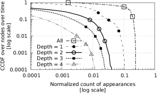
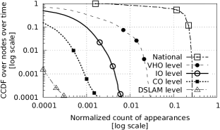
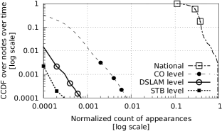
Figure 1: For each level in the hierarchy, the complementary cumulative distribution function of the normalized count of cases across nodes and time units. (a) trouble issues of CCD, (b) network locations of CCD, and (c) network locations of SCD. Note that both x- and y-axes are log scale.

II-A Operational Datasets

The data used in this study was obtained from a major broadband provider of bundled Internet, TV and VoIP services in the US. We present the results based on the datasets collected from May to September $2010$. Two distinct operational datasets were used, which we now describe.

Customer Care Call Dataset (CCD): The study used data derived from calls to the broadband service customer care center. A record is generated for each such call. Based on the conversation with the customer, the care representative assigns a category to the call, choosing from amongst a set of predetermined hierarchical classes. We focus on analyzing customer calls that are related to performance troubles (service disruptions/degradation, intermittent connectivity, etc.) and discard records unrelated to performance issues (e.g., calls about provisioning, billing, accounting). The resulting operator-assigned category constitutes a trouble description, which is drawn from a hierarchical tree with a height of $5$ levels. We summarize the distribution of the number of customer tickets for the first-level categories (Table I). Each record also specifies information concerning the network path to the customer premises, which is drawn from a hierarchical tree comprising $5$ levels.

TABLE I: CCD customer calls

Ticket Types	Percentage ($\%$)
TV	$39.59$
All Products	$26.71$
Internet	$10.04$
Wireless	$9.26$
Phone	$8.46$
Email	$3.59$
Remote Control	$2.35$

TABLE II: Hierarchy properties

Data	Type	Depth	Typical degree at $k$th level
			$k=1$	$k=2$	$k=3$	$k=4$
CCD	Trouble descr.	$5$	$9$	$6$	$3$	$5$
	Network path	$5$	$61$	$5$	$6$	$24$
SCD	Network path	$4$	$2$,$000$	$30$	$6$	N/A

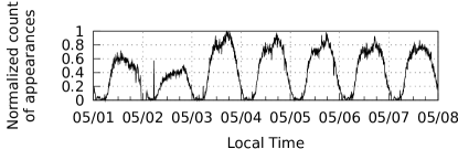
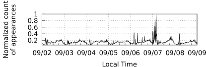
Figure 2: Two representative time series of the count of appearances in a $15$-minute precision for the datasets (a) CCD and (b) SCD. The data count is normalized, by dividing it by the maximal count in the time series. (a) and (b) starts from Saturday and Thursday, respectively.

STB Crash Dataset (SCD): At the customer premises, a Residential Gateway serves as a modem and connects to one or more Set-Top Boxes (STBs) that serve TVs and enable user control of the service. Similar to other types of computer devices, an STB may crash, then subsequently reboot. This study used logs of STB crash events from the same broadband network, that are generated by the STB. By combining the STB identifier reported in the log, with network configuration information, network path information similar to that described for CCD can be associated with each crash event. This information is represented in a hierarchical tree of $4$ levels. The broad properties such as node degrees in different levels are summarized (Table II).

II-B Characteristics of Operational Data

Sparsity: We measure the case arrival rate for difference aggregates in the hierarchies (Fig. 1). The number of cases per node, especially for nodes in the lower levels, is very sparse over time in both data sets. For example, we observe that in about $93\%$ ($70\%$) of the time we have no cases for nodes in the CO level in CCD (SCD). Anomaly detection over sparse data is usually inaccurate as it is hard to differentiate the anomalous and normal case [12]. However, larger localized bursts of calls relating to certain nodes do occur; these are obvious candidates for anomalies.

Volatility: In both datasets, we observe the number of cases varies significantly over time. For example, consider the root node of trouble issues in CCD (“All” in Fig. 1), we observe that the case number at the $90^{\mathrm{th}}$ percentile of the appearance count distribution is $\approx\!35$ times higher than that at the $10^{\mathrm{th}}$ percentile. We observe that the sibling nodes (nodes that share a common parent) in the hierarchy could have very different case arrival rates. The above observations imply that the set of heavy hitters could change significantly over time. Therefore, observing any fixed subset of nodes in the hierarchy could easily miss significant anomalies.

Seasonality: To observe the variation on arrival case counts, we measured the time series of the normalized count of appearances in $15$-minute time units (Fig. 2). Overall, a diurnal pattern is clearly visible in both the datasets. This pattern is especially strong in CCD. In particular, the daily peaks are usually around $4$ PM, while the daily minimum is at around $4$ AM. Moreover, the weekly pattern is observed in CCD where we have fewer cases in first two days (May $1-2$, 2010), which are Saturday and Sunday (Fig. 2). Regardless of the differences observed in the two datasets, one common property is the presence of large spikes. Some spikes last only a short period (e.g., $<$$30$ minutes at $5$ AM, May $2$nd in Fig. 2), while some spikes last longer (e.g., $>$$5$ hours at off-peak time, Sept $7$th in Fig. 2). These spikes are by no means unique over time – we observed a similar pattern in other time periods.

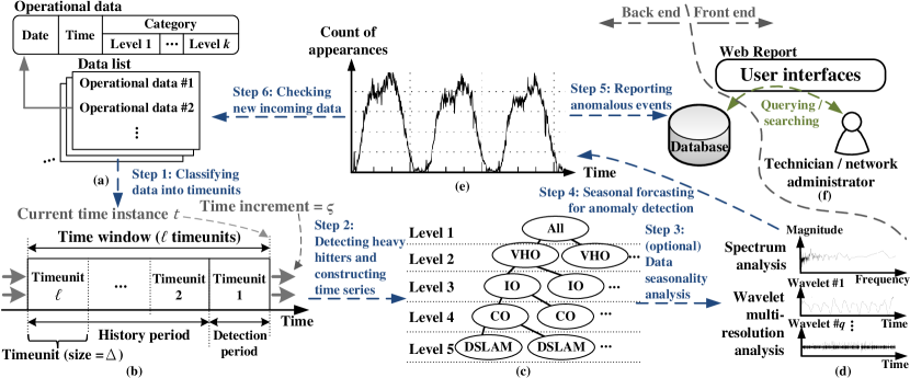
Figure 3: System diagram: (a) abstraction of streaming operational data, (b) a window-based structure to classify input data into time units, (c) heavy hitter detection and time series construction in a hierarchical domain, (d) data seasonality analysis, (e) seasonal forecasting model for anomaly detection, and (f) a user interface enables an administrator to query for anomalous events. For details, refer to §IV.

III Problem Statement

In this section, we formally define the online anomaly detection problem. In particular, we first describe the operational data format, and then we define hierarchical heavy hitter which allows us to identify the high-impact aggregates. To detect if the event related to these heavy hitters is anomalous, we define time series based anomaly detection.

An input stream ${S}=s_{0},s_{1},\dots$ is a sequence of operational network data $s_{i}$. Each data $s_{i}=(k_{i},t_{i})$ consists of two components: category $k_{i}$ provides classification information about the data; time $t_{i}$ denotes the recorded date and time of $s_{i}$. The data can be classified into “timeunits” based on its time information $t_{i}$. The data category is drawn from a hierarchical domain (i.e., tree) where each node $n$ in the tree is associated with a weight value $A_{n}[k,t]$ for timeunit $t$. For leaf nodes, the weight $A_{n}[k,t]$ is defined by the number of data items in ${S}$ whose category is $k$ and occur in timeunit $t$. For non-leaf nodes (i.e., interior nodes), the weight $A_{n}[k,t]$ is the summation of the weights of its children. We defined the hierarchical heavy hitter (HHH) as follows:

Definition 1

(HHH; Hierarchical Heavy Hitter). Consider a hierarchical tree where each node $n$ is weighted by $A_{n}[k,t]$ for timeunit $t$. Then the set of HHH for timeunit $t$ can be defined by ${HHH}[\theta,t]=\{n|A_{n}[k,t]\geq\theta\}$ for a threshold $\theta$.

These heavy hitters (i.e., high-volume aggregates) are suspicious locations where anomalies (i.e., significant spikes) could happen.

In Definition 1, the count of appearances of any leaf node will contribute to all its ancestors. Therefore, if we perform anomaly detection without taking the hierarchy into account, an anomaly in a leaf node may be reported multiple times (at each of its ancestors). To address this, one could reduce the redundancy by removing a heavy hitter node $n$ if its weight can be inferred from that of heavy hitter node $n_{d}$ that is a descendant of $n$. To arrive at this more “compact” representation, we consider a more strict definition of HHHs to find nodes whose weight is no less than $\theta$, after discounting the weights from descendants that are themselves HHHs.

Definition 2

(SHHH; Succinct Hierarchical Heavy Hitter). Consider a hierarchical tree where each node $n$ is associated with a modified weight value $W_{n}[k,t]$ for timeunit $t$. For leaf nodes, the modified weight $W_{n}[k,t]$ is equal to the original weight $A_{n}[k,t]$. For non-leaf (internal) nodes, the modified weight $W_{n}[k,t]$ is the summation of weights of its children that are themselves not a heavy hitter; In other words, given the set of SHHHs, denoted by ${SHHH}[\theta,t]$, the modified weight for non-leaf nodes can be derived by

$$W_{n}[k,t]=\sum_{m}W_{m}[k,t]:m\in child(n)\cap m\notin{SHHH}[\theta,t]$$

and the succinct hierarchical heavy hitter set is defined by ${SHHH}[\theta,t]=\{n|W_{n}[k,t]\geq\theta\}$.

Notice that both the set of SHHHs and the modified weights are unique, i.e., there can be only one heavy hitter set satisfying the above recursive definition. An intuitive explanation is that the question of whether each node joins the set only depends on the weight of its descendants. It is not hard to see that a bottom-up traversal on the hierarchy would give the correct set. We will use this definition throughout this paper (for brevity, we will write “heavy hitter” instead of “succinct hierarchical heavy hitter” hereafter).

To detect anomalous events, we will construct forecasting models on heavy hitter nodes to detect anomalous events. As heavy hitter nodes could change over time instances, we need to construct the time series only for nodes which are heavy hitters in the most recent timeunit.

Definition 3

(Time Series). For each timeunit $t$, consider a hierarchical tree where each node $n$ is weighted by $A_{n}[k,t]$. Given the heavy hitter set in the last timeunit ($t=1$), i.e., ${SHHH}[\theta,1]$, the time series of any heavy hitter node $n\in{SHHH}[\theta,1]$ is denoted by $T[n,t]=A_{n}[k,t]-\sum_{m}A_{m}[k,t]:m\in child(n)\cap m\in{SHHH}[\theta,1]$, for $1\leq t\leq\ell$, where $\ell$ is the length of time series.

Definition 4

(Anomaly). Given a time series $T[n,t]$ of any node $n$, $1\leq t\leq\ell$, the forecast traffic of the latest time period $T[n,1]$ is given by $F[n,1]$, derived by some forecasting model. Then there is an anomalous event happening at node $n$ in the latest time period iff $T[n,1]/F[n,1]>RT$ and $T[n,1]-F[n,1]>DT$, where $RT$ and $DT$ are sensitivity thresholds, which are selected by sensitivity test (§VII). We consider both absolute and relative differences to minimize false detections at peak and dip time.

IV TIRESIAS System Overview

We present our system diagram in Fig. 3. For each successive time period we receive a data list consisting of a set of newly arrived operational data (Fig. 3(a)).
Step $1$: We maintain a sliding time window to group the input streaming data into “timeunits” based on its time information $t_{i}$ (Fig. 3(b)). In particular, a time window consists of $\ell$ units, each of which is of size $\Delta$. When new data lists arrived, we simply shift the time instance / window (by a configurable offset $\varsigma$) to keep track of newly available data. For each time instance / window, we focus on detecting anomalous events in the last timeunit (the detection period in Fig. 3(b)), while the data in other timeunits is used as the history for forecasting (the history period in Fig. 3(b)).
Step $2$: Based on the category information $k_{i}$ on the data, we construct a classification tree (Fig. 3(c)), where each category $k_{i}$ can be bijectively mapping to a leaf node in the tree. As nodes associated with higher aggregated data counts in the last timeunit are suspicious places where anomaly could happen, we first detect the heavy hitter set in the classification tree (Fig. 3(c); Definition 2). Then we construct time series for these heavy hitters (Definition 3). We will present efficient algorithms to achieve these goals (§V).
Step $3$: We perform data seasonality analysis (Fig. 3(d)) to automatically choose seasonal factors. In particular, we apply fast fourier transform and à-trous wavelet transform [13] to identify significant seasonal factors (§VI). The results are used as the parameters for anomaly detection in the next step.
Step $4$: Given the time series and its seasonalities, we apply time series based anomaly detection (Fig. 3(e); Definition 4) on heavy hitter nodes. In particular, we apply the Holt-Winters’ seasonal forecasting model [14] to detect anomalies (§VI).
Step $5$: We report anomalous events to a database. A Web-based front-end system (Fig. 3(f)) is developed in JavaScript to allow SQL queries from a text database.
Step $6$: As we consider an online problem where the data arrives in a certain time period, we keep checking if new incoming data is arrived.

IV-A Limitations

Naturally, the power of Tiresias is limited by the operational data we have. We use a customer care call dataset to illustrate some of the fundamental limitations.

First, Tiresias can only detect network incidents that directly or indirectly affect customers. For example, Tiresias cannot detect upticks in memory utilization on aggregate routers if it has no sensible impact to customers. This will require a more powerful detector which has access to runtime memory usage.

Second, it is difficult to verify whether the customer call cases have been miscategorized. For example, Tiresias cannot locate an anomaly correctly if a majority of customers provide incorrect information about their geographical location. To minimize the human error, well-trained service representatives will classify the problem based on the predefined categories. We believe that the selection is much less prone to error than mining natural language.

Third, Tiresias can only process input data which is drawn from an additive hierarchy. We limit our focus on hierarchical domains as it reflects the nature of the operational datasets we had in practice (§II-A). The more general data representation (e.g., directed acyclic graph) is out scope of this paper and is left for future work.

Finally, Tiresias cannot detect anomalies where the data rate abruptly drops, for example, link outages in network traffic data [15]. We did not consider this particular type of anomalies because detecting spikes (i.e., unexpectedly increases) is much more interesting in operational data like customer care calls.

V Online HHH Detection and Time Series Construction

While we presented our system overview in the previous section, it is still unclear how to efficiently detect the heavy hitters and construct time series in an online fashion (Step $2$ in Fig. 3). To motivate our design, we start by presenting a strawman proposal STA (§V-A). Since the heavy hitter set may vary over timeunits, STA reconstructs the time series for new heavy hitters by traversing each timeunit within the sliding window of history. This requires to maintain $\ell$ trees at any time. Moreover, whenever the sliding window shifts forward, we need to traverse all of these $\ell$ trees to construct a time series for each heavy hitter. This is inefficient in time and space as the length of the time window $\ell$ (in terms of the timeunit size $\Delta$) is usually a large number, resulting in an inefficient algorithm. While this overhead can be reduced by increasing $\Delta$, or reducing the amount of history, doing so also reduces the accuracy of inference. The typical value of $\ell$ is $8$,$064$ (a $12$-week time window that is long enough to accurately construct forecasting model, and a $15$-minute timeunits that is short enough to react to operational issues). To solve this problem, we propose ADA, a novel algorithm which works by adaptively update the previous time series’ position in the hierarchy (§V-B).

V-A A Strawman Proposal STA

1 for time instance $t=t_{1},t_{1}+\Delta,t_{1}+2\Delta,\dots$ do

2       if $(t==t_{1})$ then  $\kappa=\ell$; ;

3       else  $\kappa=1$; ;

4      

5       foreach timeunit $1\leq i\leq\kappa$ do

6             Read any data item within time period $[t-i\Delta,t-i\Delta+\Delta)$ from the input stream to construct a tree ${Tree}[t-i\Delta]$ such that each node in the tree is associated with a count of appearances; Notice that we use ${Tree}[\tau]$ to represent a tree constructed by the data within time period $(\tau,\tau+\Delta]$.

7       end foreach

8      Do a bottom-up traversal on ${Tree}[t-\Delta]$ to derive the ${SHHH}[\theta,t-\Delta]$;

9       foreach timeunit $1\leq i\leq\ell$ do

10             Given the fixed heavy hitter set ${SHHH}[\theta,t-\Delta]$, do a bottom-up traversal on ${Tree}[t-i\Delta]$ to compute time series $T[n,i]$ for each node $n\in{SHHH}[\theta,t-\Delta]$;

11       end foreach

12      

13 end for

Algorithm 1 Strawman Algorithm STA.

We first describe a strawman algorithm STA (Fig. 1), which reuses the same data structure in different time instances, i.e., we destroy a tree iff it will not be used in the next time instance. While in the first iteration (i.e., $t=t_{1}$) we construct $\ell$ trees, the time spent on the first time instance can be amortized to other time instances where we construct only one tree. However, the time complexity of STA is dominated by time series construction (lines 7-9). In particular, for each time instance we need to traverse $\ell$ trees to construct a time series for each heavy hitter.

V-B A Low-Complexity Adaptive Scheme

In this section, we propose ADA, an adaptive scheme that greatly reduces the running time while simultaneously retaining high accuracy. First, we present the data structure and the pseudocode (§V-B1) for ADA. In particular, ADA maintains only one tree (rather than $\ell$ trees in STA), and only those heavy hitter nodes in the tree associated with a time series. However, the key challenge is that heavy hitters changes over time – we need efficient operations (instead of traversing $\ell$ trees) to derive the time series for heavy hitters nodes in the current time instance. To this end, we construct time series by adapting the time series generated in the previous time instance (§V-B2). For example, consider a tree with only three nodes: a root node and its two children. Suppose the root node is a heavy hitter only in the current time instance, while the two children are heavy hitters only in the last time instance. In this case, we can derive the root node’s time series by merging the time series from its two children. Although the adaptation process is very intuitive in the above example, the problem becomes more complicated as tree height increases. We will show the proposed algorithm always finds the correct heavy hitter set (§V-B3). While the positions of heavy hitters are perfectly correct, the corresponding time series might be biased after performing the split function. To address this problem, we will present two heuristics (§V-B4–§V-B5) to improve the accuracy.

Without loss of generality we assume that the time instance will keep increasing by a constant $\varsigma\leq\Delta$, where $\Delta$ is the timeunit size. We can always map the problem with time increment $\varsigma>\Delta$ to another equivalent problem with using a smaller time increment $\varsigma^{\prime}\leq\Delta$ such that $\varsigma^{\prime}$ is a divisor of $\varsigma$. For simplicity, we describe our algorithm by assuming $\varsigma=\Delta$. We further propose a recursive procedure to consider any $\varsigma\leq\Delta$ where $\varsigma$ is a divisor of $\Delta$ (§V-B6).

V-B1 Data structure and Pseudocode

We maintain a tree-based data structure as follows. Each node $n$ in the tree is associated with a type field $n.{type}$. Fields $n.{child}[i]$ and $n.{parent}$ point to the $i$-th child and parent of the node, $n.{depth}$ represents the depth of the node, and $n.{weight}$ maintains the modified weight of the node (after discounting the weight from other descendants that are themselves heavy hitters; Definition 2). Array $n.{actual}$ stores the time series of the modified weights for the node $n$, and Array $n.{forecast}$ stores the time series of the forecasted values for the node $n$.

1 for time instance $t=t_{1},t_{1}+\Delta,t_{1}+2\Delta,\dots$ do

2       if $(t==t_{1})$ then

3             Perform the same operations as lines 2-9 in STA. This gives us a tree ${Tree}$ and a heavy hitter set ${SHHH}$; We set $n.$ishh by $true$ if $n\in{SHHH}$. Otherwise, we set $n.{ishh}$ by $false$. Each heavy hitter node $n\in{SHHH}$ also has a time series of actual values $n.{actual}$ and a time series of forecast values $n.{forecast}$;

4             continue;

5            

6       end if

7      foreach node $n\in{Tree}$ do

8             $n.$washh $\leftarrow$ $n.$ishh; $n.$weight $\leftarrow$ $0$; $n.$tosplit $\leftarrow$ $0$;

9            

10       end foreach

11      foreach streaming item $(key,time)$ such that $t-\Delta\leq time<t$ do

12             Find the node $n$ such that $n.$type $==key$. Increase $n.$weight by $1$;

13       end foreach

14      Update-Ishh-and-Weight($n_{\textrm{root}}$); // Update $n.{ishh}$ and $n.{weight}$

15      

16      foreach node $n\in{Tree}$ (bottom-up level order traversal) do

17             if $(n.{ishh}\vee n.{tosplit}\wedge n\notin{SHHH})$ then

18                   $n.{parent}.{tosplit}\leftarrow true$;

19                  

20             end if

21            

22       end foreach

23      foreach node $n\in{Tree}$ (top-down level order traversal) do

24             if $((n\in{SHHH}\vee n.{depth}==1)\wedge n.{tosplit})$ then  SPLIT($n$);

25             ;

26            

27       end foreach

28      foreach node $n\in{Tree}$ (bottom-up level order traversal) do

29             if $(n\in{SHHH}\wedge\neg n.{ishh})$ then  MERGE($n$);

30             ;

31            

32       end foreach

33      if  $(n_{\textrm{root}}.{weight}<\theta)$  then  ${SHHH}\leftarrow{SHHH}\setminus n_{\textrm{root}}$;

34       ;

35       else  ${SHHH}\leftarrow{SHHH}\cup n_{\textrm{root}}$;

36       ;

37       foreach node $n\in{SHHH}$ do

38             Append $n.{weight}$ to $n.{actual}$; Remove the first element from $n.{actual}$ and that from $n.{forecast}$;

39             Derive the newest forecast value and append it to $n.{forecast}$;

40            

41       end foreach

42      

43 end for

Algorithm 2 Core Algorithm of ADA. This algorithm calls three functions: Update-Ishh-and-Weight (Fig. 3), SPLIT (Fig. 4) and MERGE (Fig. 5).

int Update-Ishh-and-Weight(node $n$)

11 foreach node $n_{c}=n.{child}$ do

      22 $n.{weight}\leftarrow n.{weight}+\textrm{Update-Ishh-and-Weight}(n_{c})$;

      

33if  $(n.{weight}\geq\theta)$  then

      44 $n.{ishh}\leftarrow 1$; return $0$;

      

55else

      66 $n.{ishh}\leftarrow 0$; return $n.{weight}$;

      

Algorithm 3 Updating fields ${n.{ishh}}$ and ${n.{weight}}$. This function recursively updates ${n.{ishh}}$ and ${n.{weight}}$ in a bottom-up fashion.

SPLIT(node $n$)

11 ${C}_{n}\leftarrow\{n_{c}|n_{c}\in n.{children}[\cdot],n_{c}\notin{SHHH}\}$;

22 if $(\exists n_{c}\in{C}_{n}\textrm{~{}s.t.~{}}n_{c}.{weight}\geq\theta)$ then

      33 foreach node $n_{c}\in{C}_{n}$ do

            44 Split the time series from $n$ to $n_{c}$ with a scale ratio of ${F}(n_{c},{C}_{n})$; (The function ${F}(\cdot)$ is defined in §V-B4)

            

      55Clear $n.{weight}$;

      66 ${SHHH}\leftarrow({SHHH}\cup{C}_{n})\setminus\{n\}$;

      

Algorithm 4 Splitting time series to children.

MERGE(node $n$)

11 if  ($n.{weight}<\theta$)  then

      22 $n_{p}\leftarrow n.{parent}$; ${C}_{n}\leftarrow\{n_{c}|n_{c}\in\{n_{p}\}\cup n_{p}.{children}[\cdot],n_{c}\in{SHHH},n_{c}.{weight}<\theta\}$;

      33 $n_{p}.{weight}\leftarrow\sum_{n_{c}\in{C}_{n}}n_{c}.{weight}$;

      44 ${SHHH}\leftarrow({SHHH}\setminus{C}_{n})\cup\{n_{p}\}$;

      55 Merge the time series from every $n_{c}\in{C}_{n}$ to $n$;

      

Algorithm 5 Merging time series to parent.

Now we describe the core algorithm of ADA (Fig. 2). We maintain a tree structure ${Tree}$ and a set of heavy hitter nodes, denoted by ${SHHH}$ over time instances. For the first time instance (lines 2-5), ADA performs the same operations as STA. However, starting from the second time instance (lines 6-29), ADA consists of the following three stages.
Initialization (lines 6-12): We reset variables $n.{washh}$, $n.{ishh}$, and $n.{weight}$. Subsequently, we recursively call a function Update-Ishh-and-Weight($n$) (Fig. 3) to calculate the $n.{ishh}$ and $n.{weight}$ according to the Definition 2.
SHHH and Time Series Adaptations (lines 13-25): Unlike STA, where we explicitly update ${SHHH}$ using a bottom-up traversal, in this stage we present a novel way to derive the set of SHHH. We first perform an inverse level order traversal (bottom-up) to check which node should “split” its time series to the children ($n.{tosplit}$). Then we perform a top-down level order traversal to split (§V-B2) the time series of any node $n$ with $n.{tosplit}$ to its children. We then do a bottom-up level order traversal to check if we should “merge” (§V-B2) the time series from some neighboring nodes to the parent. Throughout these split and merge operations, we keep updating ${SHHH}$ so that any node $n\in{SHHH}$ iff $n$ has time series $n.{actual}$ and $n.{forecast}$ (except for the root node). Finally, we simply add/remove the root node to/from ${SHHH}$ based on its weight. We will show that ${SHHH}$ satisfies the Definition 2 after performing this stage (§V-B3).
Time Series Update (lines 26-29). We update the time series for each heavy hitter node in ${SHHH}$. Unlike STA, the time series can be updated in constant time.

V-B2 S p l i t and Merge

This section presents two functions, split and merge, to adapt the position of heavy hitter nodes. Before the adaptation, heavy hitter nodes are placed in the location given in the previous timeunit. The goal is to move these heavy hitter nodes (with the binding time series and forecast) to their new positions according to the data in the current timeunit, to satisfy the Definition 2.

We leverage a SPLIT($n$) function (Fig. 4) to linearly decompose the time series from node $n$ into its non-heavy-hitter children. In other words, a heavy hitter node $n$ will be split into one or more heavy hitters in the lower level. In this function, we first check if there exists any child node $n_{c}\notin{SHHH}$ with weight $\geq\theta$. If so, we split the time series of $n$ with a scale ratio of ${F}(n_{c},{C}_{n})$ for each non-heavy-hitter child $n_{c}$ to approximate the time series of its children. We will discuss different heuristics to estimate scale ratio ${F}(n_{c},{C}_{n})$ (§V-B4).

We present a MERGE($n$) function (Fig. 5) to combine the time series from one or more lower level nodes to a higher level node. In this function, we first check if the weight of the node $n$ is smaller than $\theta$. If so, we merge the time series of $n$ and its siblings and parent who meet the same requirement as $n$.

V-B3 Correctness of Heavy Hitter Set

It suffices to show that Tiresias always selects the correct heavy hitter set after performing the stage “${SHHH}$ and Time Series Adaptation” (lines 13-21), i.e., Definition 2 will hold. The high-level intuition is that top-down split operations ensure that there is no heavy hitter hidden in the lower levels, while bottom-up merge operations ensure all non-heavy-hitter nodes propagate the weight to its heavy hitter ancestor correctly. The proof is given by Lemma 1.

Lemma 1

For each time instance, after the adaptations we have $n.{ishh}$ iff $n\in{SHHH}$ for any node $n\in{Tree}$.

V-B4 Split Rules and Error Estimation

Recall that in SPLIT($n$) function (Fig. 4), we split the time series from node $n$ to each non-heavy-hitter children $n_{c}\in{C}_{n}$ with a scale ratio of ${F}(n_{c},{C}_{n})$, where ${C}_{n}=\{n_{c}|n_{c}\in n.{children}[\cdot],n_{c}\notin{SHHH}\}$. The scale ratio is derived by ${F}(n_{c},{C}_{n})=X_{n_{c}}/\sum_{\forall m\in{C}_{n}}X_{m}$, where $X_{n}$ is a weight-related property of node $n$. Below we consider four split rules for deriving the scale ratio.

Uniform: each element in the time series of $n$ is uniformly split to all its children $n_{c}\notin{SHHH}$, i.e., $X_{n}=1$.

Last-Time-Unit: we assign $X_{n}$ by the weight of node $n$ in the previous timeunit. This assumes the weight is similar in the current timeunit and the previous one.

Long-Term-History: we assign $X_{n}$ by the total weight seen by the node across all previous timeunits.

EWMA: The Last-Time-Unit only captures the distribution in the last timeunit, while the Long-Term-History treats past observations equally. This heuristic takes a different approach – the $X_{n}$ is assigned by an exponentially smoothed weight.

We next discuss the estimation error of the “split” operation over time. For simplicity, we illustrate this by considering a EWMA-based forecast model $F[t]=\alpha T[i-1]+(1-\alpha)F[t-1]$, where $T[t]$ is the actual time series. Suppose we did a split for any time series $T$ at time $t$. Also, suppose the forecast $F[t]$ is biased by $\xi$, i.e., the estimated forecast $F_{\mathbf{E}}[t]=F[t]+\xi$. Then after $k$ iterations, the estimated forecast can be derived by

$$F_{\textbf{E}}[t+k] = \alpha\left\{\sum_{j=1}^{k}(1-\alpha)^{j-1}T[t+k-j]\right\}$$ (1)

$$+(1-\alpha)^{k-1}(F[t]+\xi)$$

for any $k>0$. Then we have relative error

$$RE[t+k] = \frac{|F_{\textbf{E}}[t+k]-F[t+k]|}{F[t+k]}$$ (2)

As the proposed algorithm derives the forecast value in a recursive way, the inaccuracy will remain in the future forecast. However, the forecast error will exponentially decrease over time because of the exponential smoothing, and this is evident in Figure 4.

Figure 4: Relative error $RE[t+k]$ after $k$ iterations. (y-axis is $\log_{10}$ scale; $\alpha=0.5$; $T[i]=1$)

V-B5 Reference Time Series

To further reduce the time series errors induced by the split operations, we propose a simple add-on to ADA by adding a set of reference time series. Consider a node $n$ with category $k$ in the hierarchical domain, the reference time series are time series of its unmodified weight $A_{n}[k,t]$ (instead of $W_{n}[k,t]$ which discounts weights from heavy hitter descendants) and the time series of its forecast values. Now we illustrate how to use the reference time series to reduce the estimation error induced by the split operations. Suppose a node $n$ splits the time series into its children using a split rule. As split operations can be inaccurate, we assume that a child node $n_{c}$ received a “biased” time series $T[n_{c},i]$, $1\leq i\leq\ell$. If $n_{c}$ has a reference time series $T_{\textrm{REF}}[n_{c},i]$, we will replace the $T[n_{c},i]$ by $T_{\textrm{REF}}[n_{c},i]-\sum_{n^{\star}\in{N}^{\star}}T[n^{\star},i]$, $1\leq i\leq\ell$, where ${N}^{\star}$ is the set of $n_{c}$’s heavy hitter descendants, i.e., ${N}^{\star}=\{n^{\star}|n^{\star}\in{SHHH}~{}\wedge~{}n^{\star}\in desc(n_{c})\}$. We maintain the reference time series only for nodes in the top $h$ levels in the hierarchy, and the memory and detection accuracy tradeoffs are discussed (§VII-A)

V-B6 Multiple Time Scales

We now show that ADA can support any case where $\Delta$ is a multiple of $\varsigma$ by generalizing ADA to support multiple time scales: consider a vector of $\eta$ time scales where the $i$-th time scale is $\lambda^{i-1}\Delta$, $1\leq i\leq\eta$ for any two given positive integers $\lambda$ and $\eta$.

To this end, we need to maintain time series in multiple time scales. We use two-dimension dynamic arrays (i.e., vector$<$ vector$<$vol_type$>$ $>$) for fields $n.{actual}$ and $n.{forecast}$, where the first dimension represents time scales. Recall that we append the new value to the tail of time series in the single time scale case (line 27 in Fig. 2). To consider multiple timescales, we defined a recursive function UPDATE_TS($n$,$w$,$i$) to append a new value $w$ to the time series of node $n$ for the $i$-th time scale (Fig. 6). In particular, when the size of any time series in the $i$-th time scale is a multiple of $\lambda$, we sum up the last $\lambda$ elements and recursively update the weight to the ($i+1$)-th time scale. It is simple to see that UPDATE_TS($n$,$w$,$i$) will be called for every $\lambda^{i}$ timeunits, for $1\leq i\leq\eta$. Then for $\kappa$ timeunits, we will call UPDATE_TS($\cdot$) $\sum_{i=1}^{\eta}\kappa/\lambda^{i}\leq 2\kappa$ times. Therefore, the update operation remains $\Theta(1)$ amortized time for each time instance.

With multiple time scales, it suffices to show that ADA can support any case where $\Delta$ is a multiple of $\varsigma$. Consider a problem $P_{A}$ with parameters $\Delta_{A}$ and $\varsigma_{A}$. It is not hard to see that $P_{A}$ is equivalent to another problem $P_{B}$ with parameters $\Delta_{B}=\varsigma_{B}=\varsigma_{A}$ by assigning $\lambda_{B}=\Delta_{A}/\varsigma_{A}$ and $\eta_{B}=1$.

UPDATE_TS(node $n$, int $w$, int $i$)

11 $n.{forecast}[i].\textrm{push\_back}(\alpha\times w+(1-\alpha)\times n.{forecast}[i].\textrm{last()})$;

22 $n.{actual}[i].\textrm{push\_back}(w)$;

33 $s\leftarrow n.{actual}[i].\textrm{size}()$;

44 if ($i<\eta~{}\wedge~{}s=0$ (mod $\lambda$)) then

      55 $w^{\prime}\leftarrow\sum_{1\leq j\leq\lambda}n.{actual}[i][s-j]$;

      66 UPDATE_TS($n$, $w^{\prime}$, $i+1$);

      77 if ($s=\ell+\lambda$) then

            88 Do $n.{actual}[i].\textrm{pop\_head}()$ $\lambda$ times.

      

Algorithm 6 Update time series in multiple time scales.

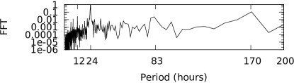
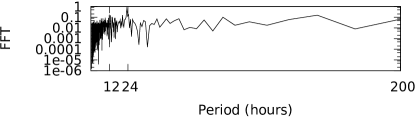
Figure 5: The Fast Fourier Transform for the datasets (a) CCD and (b) SCD. The log-scale y axis is normalized by the maximal magnitude.

VI Time Series Analysis

To study the seasonality, we apply Fast Fourier Transform (FFT) to obtain the count of appearances in frequency spectrum (Fig. 5). We observe that the most significant period is $24$ hours (i.e., day period) for both datasets, while $170$ hours (i.e., the most measurable time to the weekly period) is also noticeable in CCD. To validate this, we also perform the à-trous wavelet transform [13] to convert the time series of our datasets to “smoothed” approximations at different timescales. To avoid phase shifting, we use the low-pass $B_{3}$ spline filter $(\frac{1}{16},\frac{1}{4},\frac{3}{8},\frac{1}{4},\frac{1}{16})$ as in previous work done on time series smoothing [16]. Given the approximated time series $c_{j}(t)$ at timescale $j$, the detail of $c(t)$ at timescale $t$ can be derived by $d_{j}(t)=c_{j-1}(t)-c_{j}(t)$. Then we have the energy of the detail signal $d_{j}(t)=\sum_{\forall t}d_{j}(t)$, which indicates the strength of the fluctuations at timescale $j$. For both datasets, we apply this to multiple timescales (ranging from $5$ seconds to $4$ weeks), and the significant periodicities we found are consistent with that given by FFT. The results clearly suggest using time series model with multiple seasonalities for CCD. We found that the periodicities of operational datasets we had are fairly stable across time. Therefore, in our current implementation we perform the data seasonality analysis in an offline fashion, i.e., only in the first time instance.

To distinguish anomalous behavior, we characterize typical behavior by applying the forecasting model on time series. As we observed strong periodicities in the datasets, simple forecasting models like exponential weighted moving average (EWMA) [17] will be very inaccurate. To address this, we adopt the additive Holt-Winters’ seasonal forecasting model [14], which decouples a time series $T[t]$ into three factors: level $L[t]$, trend $B[t]$ and seasonal $S[t]$:

$$L[t] = \alpha(T[t]-S[t-\upsilon])+(1-\alpha)(L[t-1]+B[t-1])$$

$$B[t] = \beta(L[t]-L[t-1])+(1-\beta)(B[t-1])$$

$$S[t] = \gamma(T[t]-L[t])+(1-\gamma)(S[t-\upsilon])$$

where the season length is denoted by $\upsilon$. Then the forecast $G[t]$ is simply adding up these three factors, i.e., $G[t]=L[t-1]+B[t-1]+S[t-\upsilon]$. To initialize the seasonality, we assume there are at least two seasonal cycles $T[t-1],T[t-2],\dots,T[t-2\upsilon]$. The starting values $L[t-1],B[t-1]$ and $S[t-1],\dots,S[t-2\upsilon]$ can be derived by

$$L[t-1] = \frac{1}{2\upsilon}\sum_{j=t-1}^{t-2\upsilon}T[j]$$

$$B[t-1] = \frac{1}{2\upsilon}\left[\left(\sum_{j=t-1}^{\upsilon}T[j]\right)-\left(\sum_{j=t-\upsilon-1}^{2\upsilon}T[j]\right)\right]$$

$$S[t-j] = T[t-j]-L[t-1],j=1,\dots,2\upsilon$$

The use of Holt-Winters’ seasonal model does not compromise the update cost. Given the factors in the previous timeunits, the forecast can be computed in constant time. Moreover, we choose the additive Holt-Winters’ seasonal model because of its linearity – there is no need to recalculate the forecast value after merge / split.

Lemma 2

(Holt-Winter Linearity). Given $k$ Holt-Winter forecasts $G_{1}[t],G_{2}[t],G_{k}[t]$, where $G_{i}[t]=L[t-1]+B[t-1]+S[t-\upsilon]$. Consider a time series $T^{*}[t]=\sum_{i=1}^{k}T_{i}[t]$ and its Holt-Winter forecast $G^{*}[t]=L^{*}[t-1]+B^{*}[t-1]+S^{*}[t-\upsilon]$. Then $G^{*}[t]=\sum_{i=1}^{k}G_{i}[t]$.

Proof:

We prove $L^{*}[t]=\sum_{i=1}^{k}L_{i}[t]$, $B^{*}[t]=\sum_{i=1}^{k}B_{i}[t]$ and $S^{*}[t]=\sum_{i=1}^{k}S_{i}[t]$ by induction on $t$. For the initialization, we have

$$L^{*}[t-1] = \frac{1}{2\upsilon}\sum_{j=t-1}^{t-2\upsilon}T^{*}[j]$$ (3)

$$= \frac{1}{2\upsilon}\sum_{j=t-1}^{t-2\upsilon}\sum_{i=1}^{k}T_{i}[j]$$

$$= \sum_{i=1}^{k}\left(\frac{1}{2\upsilon}\sum_{j=t-1}^{t-2\upsilon}T_{i}[j]\right)$$

$$= \sum_{i=1}^{k}L_{i}[t-1]$$

$$B^{*}[t-1] = \frac{1}{2\upsilon}\left[\left(\sum_{j=t-1}^{\upsilon}T^{*}[j]\right)-\left(\sum_{j=t-\upsilon-1}^{2\upsilon}T^{*}[j]\right)\right]$$ (4)

$$= \frac{1}{2\upsilon}\left[\left(\sum_{j=t-1}^{\upsilon}\sum_{i=1}^{k}T_{i}[j]\right)\right.$$

$$-\left.\left(\sum_{j=t-\upsilon-1}^{2\upsilon}\sum_{i=1}^{k}T_{i}[j]\right)\right]$$

$$= \sum_{i=1}^{k}\left\{\frac{1}{2\upsilon}\left[\left(\sum_{j=t-1}^{\upsilon}T_{i}[j]\right)\right.\right.$$

$$-\left.\left.\left(\sum_{j=t-\upsilon-1}^{2\upsilon}T_{i}[j]\right)\right]\right\}$$

$$= \sum_{i=1}^{k}B_{i}[t-1]$$

For $j=1,\dots,2\upsilon$, we have

$$S^{*}[t-j] = T^{*}[t-j]-L^{*}[t-1]$$ (5)

$$= \left(\sum_{i=1}^{k}T_{i}[t-j]\right)-\left(\sum_{i=1}^{k}L_{i}[t-1]\right)$$

$$= \sum_{i=1}^{k}\left(T_{i}[t-j]-L_{i}[t-1]\right)$$

$$= \sum_{i=1}^{k}S[t-j]$$

Then we have following induction hypothesis for $j=t-1,t-2,\dots,t-2\upsilon$.

$$L^{*}[j] = \sum_{i=1}^{k}L_{i}[j]$$ (6)

$$B^{*}[j] = \sum_{i=1}^{k}B_{i}[j]$$ (7)

$$S^{*}[j] = \sum_{i=1}^{k}S_{i}[j]$$ (8)

Given the induction hypothesis, now we prove the theorem would hold when $j=t$.

$$L^{*}[t] = \alpha(T^{*}[t]-S^{*}[t-\upsilon])$$ (9)

$$+(1-\alpha)(L^{*}[t-1]+B^{*}[t-1])$$

$$= \alpha\left[\left(\sum_{i=1}^{k}T_{i}[t]\right)-\left(\sum_{i=1}^{k}S_{i}[t-\upsilon]\right)\right]+\left(1-\alpha\right)$$

$$\times\left[\left(\sum_{i=1}^{k}L_{i}[t-1]\right)+\left(\sum_{i=1}^{k}B_{i}[t-1]\right)\right]$$

$$= \sum_{i=1}^{k}\{\alpha\left(T_{i}[t]-S_{i}[t-\upsilon]\right)$$

$$+\left(1-\alpha\right)\left(L_{i}[t-1]+B_{i}[t-1]\right)\}$$

$$= \sum_{i=1}^{k}L_{i}[t]$$

$$S^{*}[t] = \gamma(T^{*}[t]-L^{*}[t])+(1-\gamma)(S^{*}[t-\upsilon])$$ (10)

$$= \gamma\left[\left(\sum_{i=1}^{k}T_{i}[t]\right)-\left(\sum_{i=1}^{k}L_{i}[t]\right)\right]$$

$$+(1-\gamma)\left(\sum_{i=1}^{k}S_{i}[t-\upsilon]\right)\textrm{~{}(by~{}(\ref{equ:hw:s:ih}), (\ref{equ:hw:l:pf}))}$$

$$= \sum_{i=1}^{k}\left\{\gamma(T_{i}[t]-L_{i}[t])+(1-\gamma)(S_{i}[t-\upsilon])\right\}$$

$$= \sum_{i=1}^{k}S_{i}[t]$$

∎

TABLE III: Summary of total running time of Tiresias in minutes with different algorithms. The running time for ADA is $5$-$14$ times less than that for ADA. The gap increases with the decrease of timeunit size.

Timeunit size ($\Delta$) in minutes		$15$		$60$
Algorithm		ADA	STA	ADA	STA
Reading Traces	Mean	$18.6~{}(74.0\%)$	$19.592~{}(5.4\%)$	$19.096~{}(89.0\%)$	$18.885~{}(16.2\%)$
	Variance	$12.493$	$11.493$	$15.802$	$12.801$
Updating Hierarchies	Mean	$4.762~{}(18.9\%)$	$0.198~{}(0.1\%)$	$1.699~{}(7.9\%)$	$0.273~{}(0.2\%)$
	Variance	$1.082$	$0.082$	$0.287$	$0.116$
Creating Time Series	Mean		$339.216~{}(93.9\%)$		$96.943~{}(83.1\%)$
	Variance		$83.114$		$86.518$
Detecting Anomalies	Mean	$1.785~{}(7.1\%)$	$2.232~{}(0.6\%)$	$0.67~{}(3.1\%)$	$0.546~{}(0.5\%)$
	Variance	$0.912$	$2.311$	$0.373$	$0.483$
Sum		$25.507~{}(100.0\%)$	$361.238~{}(100.0\%)$	$21.465~{}(100.0\%)$	$116.647~{}(100.0\%)$

VII Evaluation

To evaluate the performance of our algorithms, we build a $\mathrm{C}$$+$$+$ implementation of Tiresias, including ADA and STA. All our experimental results were conducted using a single core on a Solaris cluster with 2.4GHz processors. In our evaluation, we first study Tiresias’s system performance (§VII-A). Comparing it with the strawman proposal STA, the adaptive algorithm ADA provides (i) lower running time (by a factor of $14.2$), (ii) lower memory requirement (by a factor of $2$), (iii) time series with $<\!1\%$ absolute error, and (iv) identified anomalies with $99.7\%$ accuracy. We then compare Tiresias with a current best practice used by an ISP operational team (§VII-B). Tiresias not only detects $>$$94\%$ of the anomalies found by the reference method but also many previously unknown anomalies hidden in the lower levels.

System parameters: For SCD, we use the Holt-Winters’ seasonal model with single seasonal factor $S_{day}[t]$. To capture both diurnal and weekly patterns observed in CCD, we consider two seasonal factors $S_{day}[t]$ and $S_{week}[t]$ for CCD. To incorporate these two seasonal factors in the Holt-Winters’ model, we linearly combine the factors, i.e., the seasonal factor is defined as $S=\xi S_{day}[t]+(1-\xi)S_{week}[t]$. We choose the weight $\xi=FFT_{day}/FFT_{week}=0.76$ according to the measured magnitude $FFT_{t}$ of frequency $1/t$. To find the other parameters for the Holt-Winters’ forecasting model, we measure the mean squared error of the forecast values ($\propto\sum(actual-forecast)^{2}$) to choose the parameters in an offline fashion. The parameters with the minimal mean squared error are chosen for the evaluation throughout this section. We choose a small heavy hitter threshold $\theta$, which gives us around $125$ ($5$) heavy hitters in the “busy” (“quiet”) period in CCD, and $500$ heavy hitters in SCD. We perform a sensitivity test and chose sensitivity thresholds $RT=2.8$ and $DT=8$, which gave reasonable performance in comparison with the reference method (§VII-B).

VII-A System Performance

We first evaluate the performance of Tiresias using algorithms ADA and STA. We then present the results for CCD, and we summarize the results from SCD.

Computational Time: We use Long-Term-History as a representative heuristic as we observed very similar running time for these heuristics. In Table III, we summarize the running time of Tiresias using CCD in May 2010. We observe that ADA with $15$-minute ($1$-hour) timeunits reduces the overall running time by a factor of $14.2$ ($5.4$) as compared with STA. If we subtract the running time for reading traces (which is arguably necessary for any algorithm), we observed a factor of $49.5$ ($41.3$) improvement. To better understand why ADA has a better running time, we divide the program into four stages: Reading Traces, Updating Hierarchies, Creating Time Series and Detecting Anomalies. Among these stages, we observed that Creating Time Series is clearly a bottleneck in STA, which contributes $83.1\%$ ($93.9\%$) time of the total time of all stages for timeunits of size $15$-minute ($1$-hour). As the time complexity of this stage for STA is proportional to $\ell$, we expect the running time of this stage would be inversely proportional to the timeunit size. Fortunately, we also observe that the “per timeunit” running time of this stage with $15$-minute timeunits is slightly smaller (with a factor of $0.87$) than that with $1$-hour time units. This is because the trace we used is sparse, and therefore we have a smaller tree size when using smaller timeunits.

Memory Requirement: We evaluate memory costs for ADA (again, different split rules have very similar memory costs) and STA (Table IV). To eliminate cold-start effects, we focus on measuring space costs after a long run. We observe the memory cost of ADA is $\approx\!36\%$ of that of STA. We maintain the reference time series for any node in the top $h$ levels in the hierarchy (the root level is not included). With two levels of reference nodes, the memory cost of ADA is only $\approx\!43\%$ of that of STA.

TABLE IV: Normalized memory costs of Tiresias with different algorithms. (Normalized memory cost $=$ total memory cost $/$ average number of nodes in the tree $/$ the memory cost of each node.)

Algorithm	# ref.	Normalized
	levels ($h$)	Space
STA	N/A	$744.3$
ADA	$0$	$271.1$
	$1$	$280.2$
	$2$	$322.6$

Time Series Accuracy: As the split operations might introduce inaccuracy, we next examine how much distortion of time series we have. We conduct the experiment by leveraging the results generated by STA as the ground truth. In particular, for each timeunit $t$ in any time series $T[t]$, the absolute error is derived by $|T_{{ADA}}[t]-T_{{STA}}[t]|$. We first consider the impact of adding reference time series (Fig. 6). We observe the use of the reference time series significantly reduces the error rate. Consider Tiresias with reference time series for nodes in the top $h=1$, $2$, $3$ and $4$ levels, we have $61$, $322$, $1$,$926$ and $45$,$479$ reference time series, respectively. We observe that a large number of reference time series is not necessary as two layers of reference time series ($h=2$) already gives us a very accurate time series estimation ($\sim$$1\%$ error in Fig. 6). For $h=2$, we maintain reference time series for only $322/45$,$479$$\approx$$0.7\%$ of total nodes. Moreover, we compare the accuracy for different split rules. We observe that only Long-Term-History has slightly better accuracy, while the accuracy results of the other heuristics are fairly close. Besides, we observe the accuracy is very stable over different timeunits. While for brevity we did not present the accuracy results for every timeunit in the figure, we observe very similar results for older timeunits.

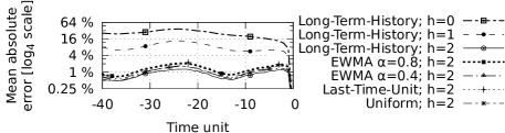
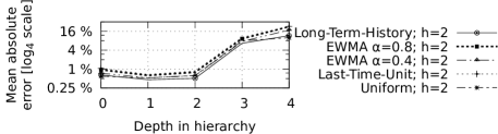
Figure 6: The absolute error of time series for different heuristics versus (a) timeunits and (b) depths. The error is averaged over different timeunits in the time series and over the time series of heavy hitters. The reference time series are not included. The timeunit $0$ is the most recent time for any time instance. We use $h$ and $\alpha$ to denote the number of reference levels (§V-B5) and the smoothing rate of EWMA, respectively.

Anomaly Detection Accuracy: We observed the heavy hitter set detected by ADA is the same as the real heavy hitter set across time. To quantify the inaccuracy introduced by the split operation, we compare the anomalies detected by ADA and STA. We use STA as the ground truth as it reconstructs accurate time series for each time instance. In Table V, we summarize the accuracy metrics for different heuristics of ADA. The results are collected across $100$ time instances between May 16-21, 2010. Overall, we found that ADA was able to detect anomalies with an accuracy of $99.7\%$ against STA. However, there are some tradeoffs between split rules. We observe that EWMA (with rate $\alpha=0.4$) has the highest precision, while Uniform has the best result on sensitivity. We also observe Long-Term-History has good results on all metrics under investigation.

Results for SCD: Compared with CCD, it takes longer running time (with a factor of $3$) for reading traces from SCD. Because of this, we observe the overall running time of ADA for SCD is slightly increased (with a factor of $1.3$). However, the overall running time of STA for SCD is greatly increased by a factor of $7.4$. In particular, the running time for Creating Time Series is increased by a factor of $6.4$ because of the increase in the size of the hierarchy. Besides, we also observe an increased memory consumption for both ADA and STA in a factor of $2$ because of the larger hierarchical space. However, with $h=0$ ($h=1$) level of reference nodes, the memory requirement of ADA is $43\%$ ($46\%$) of that of STA. For the time series accuracy of ADA, we observed an average absolute error of only $0.8\%$ with $h=1$. The primary reason of high accuracy for SCD is that the split operations are performed less frequently because of the smaller variance of the number of cases over time in SCD (Fig. 1). Consequently, we observe a very good accuracy of anomaly detection for SCD. In particular, we have no false positives and very few false negatives (in only about 0.13% of all negative cases with $h=1$).

TABLE V: Anomaly detection accuracy of Algorithm ADA. We use $h$ to denote the number of reference levels.

Split rule	$h$	Accuracy	Precision	Recall
Long-Term-History	$0$	$97.2\%$	$37.8\%$	$41.8\%$
	$1$	$98.6\%$	$78.6\%$	$49.3\%$
	$2$	$99.6\%$	$94.4\%$	$88.1\%$
EWMA $(\textrm{rate}=0.8)$	$2$	$99.6\%$	$96.5\%$	$82.8\%$
EWMA $(\textrm{rate}=0.6)$	$2$	$99.6\%$	$96.6\%$	$84.3\%$
EWMA $(\textrm{rate}=0.4)$	$2$	$99.7\%$	$96.7\%$	$87.3\%$
Last-Time-Unit	$2$	$99.6\%$	$96.5\%$	$82.8\%$
Uniform	$2$	$99.3\%$	$79.2\%$	$94.0\%$

TABLE VI: A comparison of ADA against the reference method

Performance metric	Value
Type 1 (Accuracy) $=\frac{\#\textrm{TPs}+\#\textrm{TNs}}{\#\textrm{Cases}}$	$94.1\%$
Type 2 $=\frac{\#\textrm{TPs}}{\#\textrm{TPs}+\#\textrm{MAs}}$	$90.9\%$
Type 3 $=\frac{\#\textrm{TNs}}{\#\textrm{TNs}+\#\textrm{NAs}}$	$94.1\%$

VII-B Comparison with Current Practice

To evaluate the performance of Tiresias in identifying live network problems, we compared the set of anomalies detected by our methods from CCD with a set of reference anomalies identified using an existing approach based on applying control charts to time series of aggregates at the first network level (the VHO level). This existing approach is not scaled to lower levels and is currently used by an operational team of a major US broadband provider.

For the purposes of this study we treat the reference anomalies as the ground truth against which we evaluate the performance of our method. Unfortunately, the reference anomaly set is not complete – it only looks at the anomalies that happened in the first network level (VHO). Because of this, we cannot simply use the standard terms {True$|$False} {Positive$|$Negative} in describing the anomalies found by our method relative to the reference set. To undertake the comparison, we define the following comparison metrics. Let $A_{{OP}}$ and $A_{{Tiresias}}$ denote the set of reference anomalies and those found by Tiresias, respectively. Clearly, each anomaly $a$ can be one-to-one mapping to a certain network location $L(a)$ and timeunit $T(a)$. In particular, for each anomaly $a_{{OP}}\in A_{{OP}}$, we have a true alarm (TA) case if there exists an anomaly $a_{{Tiresias}}\in A_{{Tiresias}}$ such that $T(a_{{OP}})=T(a_{{Tiresias}})$ and $L(a_{{OP}})\sqsupseteq L(a_{{Tiresias}})$, where $L_{1}\sqsupseteq L_{2}$ iff $L_{1}$ is equal to or an ancestor of $L_{2}$. In this case, Tiresias is able to locate the anomaly with finer granularity. For each anomaly in $A_{{OP}}$, we have a missed anomaly (MA) case if there does not exist any anomaly satisfying the above requirement. Moreover, let $A^{I}_{{Tiresias}}\subset A_{{Tiresias}}$ denote the set of Tiresias’s anomalies which is not related to any anomaly $a_{{OP}}\in A_{{OP}}$. Specifically, $A^{I}_{{Tiresias}}$ $=$ $\mathcal{G}(A_{{Tiresias}},A_{{OP}})$ $=$ $A_{{Tiresias}}$ $\setminus$ $\left\{a_{{Tiresias}}\in A_{{Tiresias}}|\exists a_{{OP}}\in A_{{OP}},T(a_{{OP}})=T(a_{{Tiresias}}),\right.$
$\left.L(a_{{OP}})\sqsupseteq L(a_{{Tiresias}})\right\}$. We say there is a new anomaly (NA) case for each element in $A^{I}_{{Tiresias}}$. Let $\hat{A}_{{Tiresias}}$ denote the set of heavy hitters which are not reported as anomalies by Tiresias. For each element in $\hat{a}_{{Tiresias}}\in\hat{A}_{{Tiresias}}$, we have a true negative (TN) case if $\hat{a}_{{Tiresias}}$ is unrelated to any anomaly in $A_{{OP}}$. In particular, the set of TN cases is defined by $\mathcal{G}(\hat{A}_{{Tiresias}},A_{{OP}})$, where the function $\mathcal{G}(\cdot)$ is defined in the NA case.

We compare the reported anomalies using CCD in the period of $14-24$th, September $2010$. In Table VI, we observe that ADA effectively detects most of the anomalies found by the reference method with an accuracy of $94\%$, i.e., we have a large number of true alarms and true negatives, while the number of missed anomaly is very small.

Furthermore, the results suggest that Tiresias is promising to find previous unknown anomalies. This is likely attributable to the fact that Tiresias is able to adapt heavy hitter positions to detect anomalies below the first level, whereas the reference method is only able to trace the first network level nodes. We perform a simple data aggregation of the NAs to remove any redundant anomalies which are an ancestor of other anomalies. The fraction of the resulting cases in the (VHO, IO, CO, DSLAM) level is ($5\%$, $56.3\%$, $29.3\%$, $9.4\%$). The majority ($95\%$) of NA cases are localized below the VHO level; These are inherently harder to detect with the reference dataset due to their VHO-level aggregation with non-anomalous call loads.

VIII Related work

Given the increasing severity of DoS, scanning, and other malicious traffic, traffic anomaly detection in large networks is gaining increased attention. To address this, several works detect statistical variations in traffic matrices constructed using summarizations of traffic feature distributions [18, 19]. Statistical methods used in these works include sketch-based approach [20], ARIMA modeling [21], Kalman filter [22] and wavelet-based methods [23]. ASTUTE [15] was recently proposed to achieve high detection accuracy for correlated anomalous flows. Lakhina et al. [8, 9] showed that Principal Component Analysis (PCA) can improve scaling by reducing the dimensionality over which these statistical methods operate. Huang et al. [24] proposed a novel approximation scheme for PCA which greatly reduce the communication overheads in a distributed monitoring setting. More recently, Xu et al. [25] also applied PCA to mine abnormal feature vectors in console logs. However, it is unclear how to transform hierarchical domain in operational data to multiple dimensions for PCA. While entropy of data distribution might be a useful measure as suggested in previous studies [9, 26], Ringberg et al. [27] showed that the choice of aggregation can significantly impact the detection accuracy of PCA.

There are several works on hierarchical heavy hitter detection [28, 7, 29, 11]. Among these, our earlier work [11] on hierarchical heavy hitter detection is the closest in spirit to Tiresias. However, HHD assumes cash-register model [30], where the input stream elements cannot be deleted [28]. Therefore, HHD is more useful to detect long-term heavy hitters over a coarser time granularity. To detect heavy hitters on the most recent time period, our strawman proposal STA can be seen as a nature extension of HHD where we apply HHD for every timeunit.

IX Conclusion

We develop Tiresias to detect anomalies designed toward the unique characteristics of operational data, including a novel adaptive scheme to accurately locate the anomalies using hierarchical heavy hitters. Using the operational data collected at a tier-1 ISP, our evaluation suggests that Tiresias maintains accuracy and computational efficiency that scales to large networks. We deploy our implementation on a tier-1 ISP, and our major next step is to optimize system parameters based on the feedback from ISP operational teams.

References

- [1] P. Porras, H. Saidi, and V. Yegneswaran, “A foray into Conficker’s logic and rendezvous points,” in LEET, 2009.
- [2] Z. Qian, Z. M. Mao, Y. Xie, and F. Yu, “Investigation of triangular spamming: A stealthy and efficient spamming technique,” in IEEE Symposium on Security and Privacy, 2010.
- [3] S. Stover, D. Dittrich, J. Hernandez, and S. Dietrich, “Analysis of the Storm and Nugache trojans: P2P is here.” in USENIX Magazine ;login:, 2007.
- [4] D. R. Choffnes, F. E. Bustamante, and Z. Ge, “Crowdsourcing service-level network event monitoring,” in SIGCOMM, 2010.
- [5] A. Mahimkar, J. Yates, Y. Zhang, A. Shaikh, J. Wang, Z. Ge, and C. T. Ee, “Troubleshooting chronic conditions in large IP networks,” in CoNEXT, 2008.
- [6] D. Brauckhoff, X. Dimitropoulos, A. Wagner, and K. Salamatian, “Anomaly extraction in backbone networks using association rules,” in IMC, 2009.
- [7] C. Estan, S. Savage, and G. Varghese, “Automatically inferring patterns of resource consumption in network traffic,” in SIGCOMM, 2003.
- [8] A. Lakhina, M. Crovella, and C. Diot, “Diagnosing network-wide traffic anomalies,” in SIGCOMM, 2004.
- [9] ——, “Mining anomalies using traffic feature distributions,” in SIGCOMM, 2005.
- [10] J. Zhang, J. Rexford, and J. Feigenbaum, “Learning-based anomaly detection in BGP updates,” in SIGCOMM Workshop on Mining Network Data, 2005.
- [11] Y. Zhang, S. Singh, S. Sen, N. Duffield, and C. Lund, “Online identification of hierarchical heavy hitters: Algorithms, evaluation, and applications,” in IMC, 2004.
- [12] Y. Zhao, Y. Xie, F. Yu, Q. Ke, Y. Yu, Y. Chen, and E. Gillum, “BotGraph: Large scale spamming botnet detection,” in NSDI, 2009.
- [13] M. Shensa, “The discrete wavelet transform: Wedding the à trous and mallat algorithms,” in IEEE Transactions on Signal Processing, 1992.
- [14] J. D. Brutlag, “Aberrant behavior detection in time series for network monitoring,” in USENIX Conference on System Administration, 2000.
- [15] F. Silveira, C. Diot, N. Taft, and R. Govindan, “ASTUTE: Detecting a different class of traffic anomalies,” in SIGCOMM, 2010.
- [16] K. Papagiannaki, N. Taft, Z.-L. Zhang, and C. Diot, “Long-term forecasting of Internet backbone traffic,” in INFOCOM, 2003.
- [17] C. C. Holt, “Forecasting seasonals and trends by exponentially weighted moving averages,” in International Journal of Forecasting, 2004.
- [18] G. Cormode and S. Muthukrishnan, “An improved data stream summary: the count-min sketch and its applications,” J. Algorithms, 2005.
- [19] C. Estan and G. Varghese, “New directions in traffic measurement and accounting,” in SIGCOMM, 2002.
- [20] B. Krishnamurthy, S. Sen, Y. Zhang, and Y. Chen, “Sketch-based change detection: Methods, evaluation, and applications,” in IMC, 2003.
- [21] G. E. P. Box and G. Jenkins, Time series analysis, forecasting and control. Prentice Hall, 1994.
- [22] A. Soule, K. Salamatian, and N. Taft, “Combining filtering and statistical methods for anomaly detection,” in IMC, 2005.
- [23] P. Barford and D. Plonka, “Characteristics of network traffic flow anomalies,” in SIGCOMM Workshop on Internet Measurement, 2001.
- [24] L. Huang, X. Nguyen, M. Garofalakis, J. Hellerstein, A. D. Joseph, M. Jordan, and N. Taft, “Communication-efficient online detection of network-wide anomalies,” in INFOCOM, 2007.
- [25] W. Xu, L. Huang, A. Fox, D. Patterson, and M. I. Jordan, “Detecting large-scale system problems by mining console logs,” in SOSP, 2009.
- [26] G. Nychis, V. Sekar, D. G. Andersen, H. Kim, and H. Zhang, “An empirical evaluation of entropy-based traffic anomaly detection,” in IMC, 2008.
- [27] H. Ringberg, A. Soule, J. Rexford, and C. Diot, “Sensitivity of PCA for traffic anomaly detection,” in SIGMETRICS, 2007.
- [28] G. Cormode, F. Korn, S. Muthukrishnan, and D. Srivastava, “Diamond in the rough: Finding hierarchical heavy hitters in multi-dimensional data,” in SIGMOD, 2004.
- [29] A. A. Mahimkar, Z. Ge, A. Shaikh, J. Wang, J. Yates, Y. Zhang, and Q. Zhao, “Towards automated performance diagnosis in a large IPTV network,” in SIGCOMM, 2009.
- [30] S. Muthukrishnan, “Data streams: Algorithms and applications,” in SODA, 2003.