Modeling high-energy light curves of the PSR B1259$-$63/LS 2883 binary based on 3-D SPH simulations

Abstract

Temporal changes of X-ray to very-high-energy gamma-ray emissions from the pulsar-Be star binary PSR B1259$-$63/LS 2883 are studied based on 3-D SPH simulations of pulsar wind interaction with Be-disk and wind. We focus on the periastron passage of the binary and calculate the variation of the synchrotron and inverse-Compton emissions using the simulated shock geometry and pressure distribution of the pulsar wind. The characteristic double-peaked X-ray light curve from observations is reproduced by our simulation under a dense Be disk condition (base density $\sim 10^{-9}~{}\mathrm{g~{}cm^{-3}}$). We interpret the pre- and post-periastron peaks as being due to a significant increase in the conversion efficiency from pulsar spin down power to the shock-accelerated particle energy at orbital phases when the pulsar crosses the disk before periastron passage, and when the pulsar wind creates a cavity in the disk gas after periastron passage, respectively. On the contrary, in the model TeV light curve, which also shows a double peak feature, the first peak appears around the periastron phase. The possible effects of cooling processes on the TeV light curve are briefly discussed.

1 Introduction

Recent improvement of the techniques of ground-based Cherenkov telescopes has increased the number and variety of TeV gamma-ray objects. Five gamma-ray binaries have been detected so far, with all of them known to be high mass X-ray binary systems. Their common emission mechanism has been vastly investigated since their discoveries. Each gamma-ray binary is assumed to be composed of a compact object orbiting around a massive star. Among them, PSR B1259-63/LS 2883 is the only system for which the compact object has been confirmed to be a pulsar.

PSR B1259-63 is a 48-ms radio pulsar with a spin down power of $L_{\mathrm{sd}}=8.2\times 10^{35}~{}\mathrm{erg~{}s^{-1}}$. The spectral type of LS 2883 had been known to be B2V (Johnston et al., 1994). However, a recent precise measurement reports the type to be O9.5V (Negueruela et al., 2011). This correction implies a change of the assumed distance to the system from 1.5 kpc to $2.3\pm 0.4$ kpc, as well as a change of the effective temperature of the star. The orbit has a large eccentricity $e$ of 0.87 and a long period $P_{\mathrm{orb}}$ of about 3.4 yr.

Non-pulsed and non-thermal emissions from the binary in the radio (Johnston et al., 2005; Moldón et al., 2011), X-ray (Hirayama et al., 1996; Uchiyama et al., 2009) and TeV energy ranges (Aharonian et al., 2005, 2009) have been reported, and flare-like GeV emissions were detected around the 2010–2011 periastron passage by the Large Area Telescope (LAT) on board $Fermi$ (Tam et al., 2011; Abdo et al., 2011). The radio pulse eclipse of about 5 weeks around the periastron suggests that the pulsar goes to the opposite side of the Be-disk plane with respect to the observer, while crossing it plane twice during the course. The characteristic double-peaked features observed in the radio and X-ray light curves (Connors et al., 2002; Chernyakova et al., 2006) can be mainly attributed to the interactions of the pulsar wind and the Be-disk during disk crossings by the pulsar. The peak phases or the peak intensities measured, extensively in the radio band in particular, vary from orbit to orbit, though. The observations for 2004 (Aharonian et al., 2005) and 2007 (Aharonian et al., 2009) periastron passage indicate that the TeV light curve also varies from orbit to orbit.

The non-thermal emission mechanisms of the system have been studied in the framework of leptonic (e.g., Tavani & Arons, 1997; Khangulyan et al., 2007; Sierpowska-Bartosik & Bednarek, 2008; Takata & Taam, 2009; Dubus et al., 2010) and hadronic models (Kawachi et al. 2004; see also Neronov & Chernyakova 2007). Unfortunately, Be-disk models which have been adopted so far in this field of research are mostly outdated, and are significantly different from the model being widely accepted by the Be star research community currently, i.e., the viscous decretion disk model [Lee et al. (1991); see also Porter (1999) and Carciofi & Bjorkman (2006)]. Since the shock distance and its geometry depend on the Be-disk model, it is important to examine the high-energy emissions with a more realistic Be-disk model. For instance, disk models with supersonic outflows, as adopted in most previous studies, have irrelevantly large ram pressure, and thus give rise to false location of the shock.

Detailed two-dimensional hydrodynamic simulations have also been performed to study the wind-wind collision interaction in this system (e.g., Bogovalov et al., 2008, 2011), providing important information on the shock structure. Since the simulations have been limited to 2-D, however, the orbital motion has not been taken into account, which can have significant effects near the periastron passage. Moreover, the presence of the Be-disk can play an important role to the origin of the high energy emission from this system. In such a case, the behavior of the system will inevitably manifest in 3-D and be orbital-phase dependent.

In Okazaki et al. (2011, hereafter paper I), we have studied the interaction between the pulsar and the Be star by, for the first time, carrying out 3-D hydrodynamic simulations using the viscous decretion disk model. We have found that for a Be-disk with typical density, the pulsar wind strips off an outer part of the Be-disk, truncating the disk at a radius significantly smaller than the pulsar orbit. This prohibits the pulsar from passing through the disk around periastron passage, which has been assumed in previous studies. In other words, a Be-disk with typical density is dynamically unimportant in this system.

A large H$\alpha$ equivalent width of $-54$ Å (Negueruela et al., 2011), however, suggests that the density of the Be-disk of LS 2883 is much higher than typical. It is, therefore, interesting to see how the interaction changes if the Be-disk is much denser and dynamically more important than those studied in paper I. Given the double-peaked light curves of PSR B1259-63, a particularly important issue is whether a reasonably high Be-disk density can lead to a strong pulsar wind confinement, and hence an enhanced emission, during both disk-plane crossings.

In this paper, which is the second of the series, we study high energy emissions from PSR B1259-63/LS 2883 system, based on the results of numerical simulations for different values of the Be-disk density. We review our 3-D hydrodynamic simulations in section 2 and describe our emission model in section 3. Based on the model light curves, we propose, in section 4.2, a new interpretation of the observed double-peaked feature of the radiation (in particular in the X-ray band). The multi-wavelength emission properties are discussed in section 4.3. Finally, we summarize our results in section 5.

2 Numerical Model for the Hydrodynamic Interaction between the Pulsar and the Be Star

The simulations presented below are performed with a 3-D SPH code. The code is basically identical to that used by Okazaki et al. (2002) (see also Bate et al., 1995), except that the current version is adapted to systems with winds and a decretion disk, such as PSR B1259-63/LS 2883, and takes into account radiative cooling with the cooling function generated by CLOUDY 90.01 for an optically thin plasma with solar abundances (Ferland, 1996). Using a variable smoothing length, the SPH equations with a standard cubic-spline kernel are integrated with an individual time step for each particle. In our code, the Be-disk, the Be wind, and the pulsar wind are modeled by ensembles of gas particles of different particle masses with negligible self-gravity, while the Be star and the pulsar are represented by sink particles with the appropriate gravitational masses. Gas particles which fall within a specified accretion radius are accreted by the sink particle.

To reproduce the Be decretion disk, we inject gas particles just outside of the stellar equatorial surface at a constant rate. In paper I, we adopted the injection rate of $3.5\times 10^{-9}M_{\odot}\,\mathrm{yr}^{-1}$, which gave rise to a typical disk base density of $10^{-11}\,{\rm g~{}cm}^{-3}$ [detailed model fit of the observed H$\alpha$ profiles typically provides a density between $10^{-12}\,{\rm g~{}cm}^{-3}$ and several times $10^{-10}\,{\rm g~{}cm}^{-3}$ (e.g., Silaj et al., 2010)]. In the current study, however, we compare the resulting radiation spectrum/light curve for three different injection rates, fixing all the other parameters at values adopted in paper I. Particularly, for the mass and radius of the Be star, we take values typical for a B2V star to ensure consistency with the models studied in paper I. The polar axis of the Be star is tilted from the binary orbital axis by $45\arcdeg$, and the azimuth of tilt, i.e. the azimuthal angle of the Be star’s polar axis from the direction of apastron, is $19\arcdeg$. With this geometry, the pulsar crosses the equatorial plane of the Be star at $\tau\sim-10\,\mathrm{d}$ and $\tau\sim+25\,\mathrm{d}$, where $\tau$ is the orbital phase in days relative to the periastron passage. We choose rates of $3.5\times 10^{-9}M_{\odot}\,\mathrm{yr}^{-1}$, $3.5\times 10^{-8}M_{\odot}\,\mathrm{yr}^{-1}$, and $3.5\times 10^{-7}M_{\odot}\,\mathrm{yr}^{-1}$, corresponding to disk base densities of $10^{-11}\,{\rm g~{}cm}^{-3}$, $10^{-10}\,{\rm g~{}cm}^{-3}$, and $10^{-9}\,{\rm g~{}cm}^{-3}$, respectively. Remarkably, we find that the highest injection rate is favored by best reproducing the observed light curve. We note that taking the base density of $10^{-9}\,{\rm g~{}cm}^{-3}$ for this system is not unreasonable, given that LS 2883 showed the H$\alpha$ equivalent width of $-54$ Å in quiescence (Negueruela et al., 2011), which was one of the largest equivalent widths Be stars have ever shown.

The Be wind and pulsar wind are turned on in the simulation at a certain time after the Be-disk has fully developed in the tidal simulation (for more details, see paper I). We started the wind simulation at $t=11.44\,P_{\rm orb}$, 74 days prior to periastron passage. For simplicity, we assume that the winds coast without any net external force, assuming in effect that gravitational forces are either negligible (i.e. for the pulsar wind) or are cancelled by radiative driving terms (i.e. for the Be wind). The relativistic pulsar wind is emulated by a non-relativistic flow with a velocity of $10^{4}\,{\rm kms}^{-1}$ and an adjusted mass-loss rate so as to provide the same momentum flux as a relativistic flow with the same assumed energy. We assume that all the spin down energy $L_{\rm sd}=8.2\times 10^{35}\,{\rm erg~{}s}^{-1}$ goes to the kinetic energy of a spherically symmetric pulsar wind. We also assume the Be wind to be spherically symmetric with a mass loss rate of $10^{-8}\,M_{\odot}\,{\rm yr}^{-1}$.

It is noted that the unshocked pulsar wind is emulated by a non-relativistic flow with a momentum flux ($L_{\rm sd}/c$), where $c$ is the speed of light. The global structure of pulsar wind under the influence of the Be-wind/disk should be reasonably represented by this treatment. This is because it depends primarily on the momentum flux ratio and not on whether the pulsar wind is modeled as relativistic (see paper I for details). This will justify the application since we estimate the light curve and spectrum by integrating all the contributions from each emission region. The resulting light curve and spectrum should not depend on the detailed local structure of the shocked pulsar winds. Rather, they should depend mainly on the global structure. Thus we conclude the resulting light curve and spectrum in this study are robust in spite of our non-relativistic treatment. Of course, as stated in Bogovalov et al. (2008, 2011), the relativistic effects can affect the detailed structure of unshocked/shocked pulsar wind regions. Thus it is our future plan to extend our code to the relativistic regine and examine its influence. The possibility of relativistic Doppler boost effect is discussed in section 4.1.

3 Emission Model for Shocked Pulsar Wind

We calculate the emission at each orbital phase using data from the 3-D hydrodynamic simulations. First, the simulation volume is divided into uniform grids, and at each grid point the pulsar wind pressure is calculated by counting only the contribution from the pulsar wind particles. Then, from the 3-D distribution of the pulsar wind pressure, synchrotron and inverse-Compton emissions are locally evaluated by using an assumption on the local magnetic fields and the calculation scheme described in the following subsections. In these calculations, we implicitly assume that particles are accelerated through the 1st-order Fermi mechanism at the pulsar wind termination shock, and have a power-law energy distribution. We anticipate that the motion of each SPH particle, which represents an ensemble of electrons and positrons, corresponds to the bulk motion of the pulsar wind particles represented by the SPH particle. In the down stream region, we assume that the motion of the electrons and positrons represented by each SPH particle is randomized and the energy distribution is described by the power law function (section 3.2.1).

The total emissions are obtained by integrating the local emissions over the whole simulation volume. We adopt $100^{3}$ uniform grids and have confirmed that the result does not change even if grids with higher resolution are used. Although the integration is taken over the whole simulation volume, virtually all the contribution to the high energy emission arises from the shocked pulsar wind region, because the unshocked (upstream) region of the pulsar wind is too cold to make any significant contribution to the emission. It has been suggested that the relativistic bulk motion of the upstream flow may produce a considerable high energy emissions via the inverse-Compton process. In this study, however, because our simulations are done in the non-relativistic limit, we do not investigate this point. It has been suggested that the radio emission can come from a larger volume than emissions in other wavelengths (Moldón et al., 2011). This volume is roughly $\sim$ 100 AU, which is about one order of magnitude larger than the size of the present simulation volume ($\sim 2a\sim 1.5\times 10^{14}$ cm). Estimation of emission in the radio band is hence omitted here and postponed to future studies.

3.1 Magnetic Fields

Our simulations are performed in the hydrodynamic limit and there are theoretical uncertainties involved in determining the magnetic field of the pulsar wind. The magnetic field in the shock down-stream is obtained using the Rankine-Hugoniot relations at the shock surface and the adiabatic expansion-law of ideal MHD flow as in the cases of steady nebulae (e.g. Kennel and Coroniti 1984; Tavani and Arons 1997; Nagataki 2004). The flow in our simulations, however, is too dynamic for the above calculation scheme to be applied to. Therefore, we adopt another approach frequently used in modeling gamma-ray bursts (e.g. Sari et al. 1998; Xu et al. 2011) as follows. On the pulsar side, the total pulsar wind pressure $P_{\rm tot}$ at each grid is associated with the local magnetic field $B$ as

$$B=\sqrt{\eta\times 8\pi P_{\rm tot}},$$ (1)

where $\eta$ is fixed to 0.1, which gives a X-ray flux consistent with observations of PSR B1259-63/LS 2883 system.

3.2 Scheme of Calculation

3.2.1 Energy distribution of accelerated particles

The synchrotron and inverse-Compton processes are calculated in the simulation grids where the pulsar wind pressure $P_{\mathrm{tot}}$ is non-zero and the contribution of the wind particles is $P_{\mathrm{g}}\equiv(1-\eta)P_{\mathrm{tot}}$. We assume that the number of shocked particles per Lorentz factor per volume at each grid point is given by a single power law function of

$$f(\Gamma)=\frac{K}{4\pi}\Gamma^{-p}~{}~{}(\Gamma_{\mathrm{min}}\leq\Gamma\leq\Gamma_{\mathrm{max}}),$$ (2)

where $\Gamma$ is the Lorentz factor of the particles. Note that the accelerated particles are strictly relativistic in our model, such that their momenta are simply $m_{e}c\Gamma$, where $m_{e}$ is the electron rest mass. We will therefore write down their distribution in $\Gamma$ instead of momentum for convenience.

The minimum Lorentz factor $\Gamma_{\mathrm{min}}$ is similar to the Lorentz factor of the bulk motion of the unshocked flow. At the limit of small magnetization parameter ($\sigma\ll 1$), the latter is given by $\sim\sigma_{L}\Gamma_{L}$, where $\sigma_{\mathrm{L}}$ and $\Gamma_{\mathrm{L}}$ are the magnetization parameter and the bulk Lorentz factor at the light cylinder radius of the pulsar. With $\sigma_{\mathrm{L}}\sim 10^{3}$ and $\Gamma_{\mathrm{L}}\sim 10^{2-3}$, $\Gamma_{\mathrm{min}}$ of 5$\times 10^{5}$ is obtained. The maximum Lorentz factor $\Gamma_{\mathrm{max}}$ is determined as $\Gamma_{\mathrm{max}}=\mathrm{min}(\Gamma_{\mathrm{s}},\Gamma_{\mathrm{c}})$; $\Gamma_{s}$ is the Lorentz factor at which the acceleration timescale $t_{a}\sim\Gamma m_{e}c/eB$ with $e$ being electron charge is equal to the synchrotron loss timescale $t_{s}\sim 9m_{e}^{3}c^{5}/4e^{4}B^{2}\Gamma$, whereas $\Gamma_{c}$ is defined as the Lorentz factor at which the acceleration timescale $t_{a}$ is equal to the dynamical timescale of the shocked pulsar wind $t_{c}$. Here, $t_{c}$ is deduced as $\sim h_{p}/(c/\sqrt{3})$ with the scale height $h_{p}$ of the gas pressure estimated from the simulation. The typical $\Gamma_{\mathrm{max}}$ in this work is of order 10⁸.

The energy density $\epsilon_{p}$ is related to the gas pressure $P_{g}$ as $\epsilon_{p}=3P_{g}$. Using the condition $\epsilon_{p}=m_{e}c^{2}\int\int\Gamma f(\Gamma)d\Gamma d\Omega$, we calculate the normalization factor $K$ as

$$K=\frac{3P_{g}}{m_{e}c^{2}}\left\{\begin{array}[]{@{\,}ll}\frac{2-p}{\Gamma_{\rm max}^{2-p}-\Gamma_{\rm min}^{2-p}}&\mathrm{for}~{}~{}p\neq 0\\ \left[\mathrm{ln}(\Gamma_{\rm max}/\Gamma_{\rm min})\right]^{-1}&\mathrm{for}~{}~{}p=2\end{array}\right.$$ (3)

It is well known that the standard 1st-order Fermi mechanism in the test-particle limit gives $p=(r+2)/(r-1)$, where $r$ is the compression ratio at the shock wave. Assuming a strong, non-relativistic shock, the compression ratio $r=4$ is derived from the Rankine-Hugoniot relation, so that the index$p=2$. From previous studies, in general we can expect that $p\geq 2$ for weak, non-relativistic shocks, and $1.0\leq p\leq 2.2$ for strong, relativistic shocks, respectively (see, e.g. Longair 1994 and references therein). Limited by the spatial resolution, nevertheless, it is very difficult to determine the shock conditions in the emission region directly from the hydro simulation. Therefore, unless mentioned otherwise, we will adopt $p=2$ as our canonical value for the results in this paper. In addition, cases for $p=2\pm 0.5$ will also be investigated to illustrate the possible effects of the uncertainty in $p$ on our results, in particular the multi-wavelength emission spectra.

3.2.2 Formulae

The synchrotron power per unit energy emitted by each electron is calculated according to Rybicki & Lightman (1979) as

$$P_{\rm syn}(E)=\frac{\sqrt{3}e^{2}B\sin\theta_{p}}{hm_{e}c^{2}}F_{\rm sy}\left(\frac{E}{E_{\rm syn}}\right),$$ (4)

where $E_{\rm syn}=3he\Gamma^{2}B\sin\theta_{p}/4\pi m_{e}c$ is the typical photon energy and $F_{\rm sy}(x)=x\int_{x}^{\infty}K_{5/3}(y)dy$, where $K_{5/3}$ is the modified Bessel function of order 5/3. For the pitch angle $\theta_{p}$, we use the averaged value corresponding to $\sin^{2}\theta_{P}=2/3$. The power per unit energy and per unit solid angle of the inverse-Compton process is described by (Begelman & Sikora, 1987)

$$\frac{dP_{\rm IC}}{d\Omega}={\mathcal{D}}^{2}\int_{0}^{\theta_{c}}(1-\beta\cos\theta_{0})I_{b}/h\frac{d\sigma^{\prime}_{KN}}{d\Omega^{\prime}}d\Omega_{0},$$ (5)

where $d\sigma^{\prime}/d\Omega^{\prime}$ is the differential Klein-Nishina cross section, $\beta=\sqrt{\Gamma^{2}-1}/\Gamma$, $\mathcal{D}=\Gamma^{-1}(1-\beta\cos\theta_{1})^{-1}$ with $\theta_{1}$ and $\theta_{0}$ being the angles between the direction of the particle motion and the propagating direction of the scattered photon and the background photons, respectively, $h$ is the Planck constant, $I_{b}$ is the background photon field and $\theta_{c}$ expresses the angular size of star as seen from the emission point. For the target stellar photons, a soft photon field with an effective temperature of 30,000 K is taken, and the Be-disk emission is omitted for simplicity.

For the Earth viewing angle, we assume that the inclination angle of the orbital plane with respect to the sky is $i\sim 23^{\circ}$ and the true anomaly of the direction of Earth is about $\phi\sim 130^{\circ}$ (Johnston et al. 1996; Negueruela et al. 2011). The model spectrum of the emission from the shocked wind measured at Earth is calculated as

$$F_{E}(E)\sim\frac{e^{-\tau_{\gamma\gamma}}}{D^{2}}\Sigma_{i}\left[\delta V_{i}\int_{\Gamma_{\rm min}}^{\Gamma_{\rm max}}f(\Gamma)\left(P_{\rm syn}+\int\frac{dP_{\rm IC}}{d\Omega}d\Omega\right)d\Gamma\right],$$ (6)

where $\Sigma_{i}$ expresses the summation of the each grid and $\delta V_{i}$ is the volume of the each grid. The optical depth, $\tau_{\gamma\gamma}$ for the pair-creation process between the gamma-rays emitted by the wind particles and the stellar photons is expressed by

$$\tau_{\gamma\gamma}=\int_{0}^{\infty}d\ell\int_{E_{\rm c}}^{\infty}dE_{s}\sigma_{\gamma\gamma}dN_{s}/dE_{s},$$ (7)

where $\ell$ is the propagating distance of the $\gamma$-ray from the emitted point, $dN_{s}/dE_{s}$ is the distribution of the number density of the stellar soft photon and

$$\sigma_{\gamma\gamma}(E_{\gamma},E_{s})=\frac{3}{16}\sigma_{\rm T}(1-v^{2})\left[(3-v^{4})\mathrm{ln}\frac{1+v}{1-v}-2v(2-v^{2})\right],$$ (8)

where $\sigma_{T}$ is the Thomson cross section, $v(E_{\gamma},E_{s})=\sqrt{1-E_{\rm c}/E_{\gamma}}$ and $E_{\rm c}=2(m_{e}c^{2})^{2}/[(1-\cos\theta_{\gamma\gamma})E_{s}]$ with $\theta_{\gamma\gamma}$ being the collision angle. We use the distance $D=2.5$ kpc in this work.

4 Results and Discussion

In this section, we first summarize the results of the hydrodynamic interaction between the pulsar wind and the circumstellar material of the Be star. We then present the multi-wavelength light curves and an time-averaged spectrum obtained using the simulation data. We will also briefly discuss the cooling processes and comment on our non-relativistic emulation of the relativistic pulsar wind.

4.1 Hydrodynamic Interaction between the Pulsar and the Be star

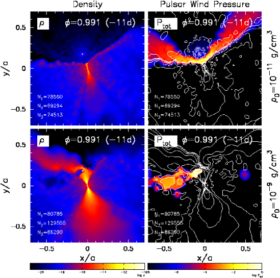
Figure 1: Snapshots taken from two SPH simulations for different base densities of the Be-disk: $\rho_{0}=10^{-11}\,\mathrm{g~{}cm}^{-3}$ (upper panels) and $\rho_{0}=10^{-9}\,\mathrm{g~{}cm}^{-3}$ (lower panels). The left and right panels show the volume density and the pulsar wind pressure, respectively, at $\tau=-11\,\mathrm{d}$ (11 days prior to the periastron). In the left panels, the locations of the Be star (the central white dot) and the pulsar (the white dot above the Be star) are also shown, while in the right panel, the volume density is denoted by contours. The density varies by one order of magnitude per contour. In each panel, $N_{1}$, $N_{2}$, and $N_{3}$ annotated at the lower left corner are the numbers of particles in the Be wind, the pulsar wind, and the Be-disk, respectively.

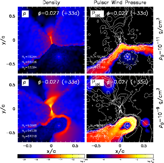
Figure 2: Same as Figure 1, but at $\tau=+33\,\mathrm{d}$ (33 days after the periastron).

As mentioned in section 2, we have run 3-D SPH simulations of hydrodynamic interaction in PSR B1259-63/LS 2883 with the base density of the Be decretion disk in the range of $10^{-9}-10^{-11}\,\mathrm{g~{}cm}^{-3}$. Figures 1 and 2 show snapshots of the interaction between the pulsar wind and the circumstellar material of the Be star in the binary orbital plane at two different epochs, 11 days prior to periastron passage ($\tau=-11~{}\mathrm{d}$) and 33 days after it ($\tau=+33~{}\mathrm{d}$), respectively. Each figure compares the shock structure in two SPH simulations with different disk base densities, $\rho_{0}=10^{-11}\,\mathrm{g~{}cm}^{-3}$ (upper panels) and $\rho_{0}=10^{-9}\,\mathrm{g~{}cm}^{-3}$ (lower panels): left and right panels show the distribution of the volume density and the pulsar wind pressure, respectively. To clarify the location where the pulsar wind is terminated, the right panel also shows the distribution of the volume density in contours. These figures highlight the effect of the Be-disk density on the geometry of the interaction surface. For $\rho_{0}=10^{-11}\,\mathrm{g~{}cm}^{-3}$, the pulsar wind easily strips off an outer part of the Be-disk, truncating the disk at a radius significantly smaller than the pulsar orbit. As a result, the interaction surface is open and covers only a small solid angle around the pulsar (Figures 1 and 2, upper panels), implying that only a small fraction of the pulsar wind energy is available for particle acceleration.

In contrast, for $\rho_{0}=10^{-9}\,\mathrm{g~{}cm}^{-3}$, the Be-disk has a large enough inertia not to be pushed away so easily by the pulsar wind. Thus, as the pulsar approaches the Be-disk before periastron passage, the distance between the interaction surface and the pulsar rapidly decreases and finally becomes smaller than the scale-height of the disk. The pulsar then penetrates the Be-disk, opening a small cavity around it. The disk gas surrounding the pulsar terminates the pulsar wind over a large solid angle, converting a large fraction of the bulk pulsar wind energy into the energy of shocked particles. After periastron, the pulsar approaches the Be-disk again, now moving away from the Be star. Since the pulsar wind pushes the disk in the direction along which the disk density decreases, it can move the disk gas more easily than it could before periastron. As a result, a slowly expanding shell is formed around the pulsar, which terminates the pulsar wind again over a large solid angle, efficiently converting the pulsar wind energy into the energy of shocked particles (Figure 2, lower panels). The details of these hydrodynamic simulations will be discussed in a subsequent paper (Okazaki et al. 2012, in prep)

4.2 X-ray Light Curves

Figure 3 presents the calculated light curves of the X-ray flux (1-10 keV energy bands) together with the observed fluxes taken from Neronov& Chernyakova (2007) as a function of days relative to the periastron passage, $\tau$. The solid, dashed and dotted lines are the results for disk base densities of $\rho_{0}=10^{-11}~{}\mathrm{g~{}cm^{-3}}$, $10^{-10}~{}\mathrm{g~{}cm^{-3}}$ and $10^{-9}~{}\mathrm{g~{}cm^{-3}}$, respectively, with the typical value of the power index $p=$2 for the accelerated particles.

During the pre-periastron period, up to $\tau=-11\,\mathrm{d}$, the flux does not depend on the disk base density. This is because the pulsar wind interacts mainly with the stellar wind, for which we assume an identical mass loss rate of $10^{-8}\,M_{\odot}\,{\rm yr}^{-1}$. The epochs during which the pulsar crosses the Be-disk plane are estimated by the simulation to be about 11 days prior to the periastron passage ($\tau\sim-11\,\mathrm{d}$) and 25 days after it ($\tau\sim+25\,\mathrm{d}$). The interaction between the pulsar wind and Be-disk is expected to be the strongest during the disk crossings.

Remarkably, however, the X-ray flux for cases of disks with typical base densities $\rho_{0}=10^{-10}-10^{-11}$ $\mathrm{g~{}cm^{-3}}$ does not peak at the timing of disk crossings, but shows a maximum intensity at the periastron. On the other hand, the X-ray flux for the highest density case ($\rho_{0}=10^{-9}~{}\mathrm{g~{}cm^{-3}}$) increases distinctively around the phases of the disk crossings, resulting in a double-peaked structure.

The dependence of the light curves on the Be-disk density reflects that of the shock geometry and resultant conversion efficiency from the spin down power to the internal energy of the shocked pulsar wind (Figure 4). For a typical disk density, we see that the pulsar wind can easily truncate the Be-disk at a radius smaller than the pulsar’s orbit. Therefore, the solid angle as measured from the pulsar, over which the pulsar wind is stopped by the Be-disk, is small. In this case, the intensity of synchrotron emission is highest at the periastron because the magnetic fields of the shocked pulsar wind are highest there (see equation (1)).

The pulsar wind cannot dismiss the disk with the higher density ($\rho_{0}=10^{-9}~{}\mathrm{g~{}cm^{-3}}$), i.e., with a large inertia. The shock is pushed back toward the pulsar in the first disk plane crossing ($\tau\sim-11\,\mathrm{d}$). After the periastron, the pulsar approaches the Be-disk again, but now moving away from the Be star. Since the pulsar wind pushes the disk in the direction along which the disk density decreases, it displaces the disk gas more easily than it did in the pre-periastron crossing. As a result, a slowly expanding shell is formed around the pulsar, which terminates the pulsar wind over a larger solid angle ($\tau\sim+33\,\mathrm{d}$). The particles at the shock obtain energy from the bulk kinetic energy of the unshocked pulsar wind, which is in turn provided by the pulsar spin down power. At these disk-plane crossing phases, the conversion efficiency from the pulsar spin down power to the shock-accelerated particle energy drastically increases, which leads to the increase in the X-ray flux, most notably in the post-periastron crossing phase (Figure 4).

We would like to stress that no fine-tuning has been done in our study for the sake of reproducing the observed X-ray light curve. Thus it is remarkable that the calculated flux level and double-peak phases for the case of $\rho_{0}=10^{-9}~{}\mathrm{g~{}cm^{-3}}$ and $\eta=0.1$ in equation (1) turn out to be very similar to those from observations, as shown in Figure 3. Our model sheds new light on the disk density as a probe of the high energy emission mechanisms. Interestingly, the favored density in this study is higher than the typical one for Be-disks.

Our model possesses a few profound features which distinguish it from previous studies. First, the present simulations predict that the conversion efficiency varies with the orbital phase, while the previous studies have assumed a constant conversion efficiency over the whole orbit (e.g., Tavani & Arons, 1997; Takata & Taam, 2009). Second, in the present model, the conversion efficiency and therefore the X-ray flux acquire the maximum values when the pulsar wind interacts with the Be-disk. In Tavani & Arons (1997), on the other hand, the inverse-Compton cooling process which dominates over other cooling processes is crucial to reproduce the observed decrease of the flux near the periastron. Takata & Taam (2009) and Kong et al. (2011) invoked the model that the pulsar wind parameters at the shock (e.g. the $\sigma$ parameter) vary throughout the orbital phase.

4.3 GeV/TeV Light Curves

Figure 5 shows the calculated light curves for 0.1-100 GeV and TeV ($>$300GeV) energy bands. We find that the gamma-ray light curves show the double-peaked structures as in their X-ray counterpart. For 0.1-100 GeV light curves, the peaks align with those in the X-ray bands, because both X-ray and 100 MeV-1 GeV emissions are produced by the synchrotron process. In the recent results from $Fermi$ (Tam et al., 2011; Abdo et al., 2011), however, it is likely that the phases of the peaks in the X-ray and the GeV bands do not align with each other. Furthermore, $Fermi$ has not detected a strong and sharp peak before the periastron, which is seen in the present model. Hence, in the present framework, there are some discrepancies between the properties of the calculated and observed GeV light curves. We would like to note that the 0.1-1 GeV flux particularly depend on the magnetic field, because the synchrotron spectrum from the shocked particles has a cut-off around 1-200 MeV. In the present model, if the maximum Lorentz factor is determined by the balance between the synchrotron cooling timescale and the acceleration timescale, the maximum Lorentz factor of the particles is expressed as $\Gamma_{\mathrm{s}}\sim(9m_{e}^{2}c^{4}/4e^{3}B)^{1/2}$, which indicates the synchrotron photon energy of $E_{\mathrm{syn}}=3\Gamma_{\mathrm{s}}^{2}eB\sin\theta_{p}/(4\pi m_{e}c)\sim 3^{5/2}m_{e}c^{3}h/(2^{7/2}\pi e^{2})\sim 200$ MeV. For a lower magnetic field, the maximum Lorentz factor may be determined by the balance between the acceleration timescale and the dynamical timescale of the shocked pulsar wind. In such a case, the cut-off energy of the synchrotron radiation is $E<E_{\mathrm{syn}}\sim 200$ MeV, and the 0.1-1 GeV flux is sensitive to the magnetic field. Furthermore, contributions by emissions from the high-order generated pairs (Sierpowska-Bartosik & Bednarek, 2008) and the inverse-Compton emission from the unshocked pulsar wind (e.g., Khangulyan et al., 2011a) to the observed spectrum below the TeV band have been pointed out. Therefore, a more detailed modeling of the 0.1-100 GeV emission process is necessary for a closer comparison with the $Fermi$ results.

For the TeV emissions, which are produced by the inverse-Compton process, we can see in Figure 5 that the second peak of the light curve aligns with that of the X-ray band, whereas the first peak comes around near the periastron. The timing of the first peak of the TeV lightcurve reflects the fact that the stellar soft-photon field strength at the emission region (that is, the shock) reaches its maximum during periastron passage. As we described in section 4.2, though the conversion efficiency from the spin down energy to the particles energy of the shocked wind decreases as the pulsar moves toward the periastron, the effect of the increasing strength of the soft photon fields toward the periastron outweighs the decrease of the conversion efficiency. The periastron peak does not well reproduce the observations, at least of the 2004 periastron passage.

It is shown in Figure 5 that the light curve in the $>$ 300 GeV band suffers from photon-photon absorption where soft photons are assumed to come only from the Be star. In the present calculation, we have taken a spherically symmetric stellar photon field. However, Negueruela et al. (2011) estimated a stellar temperature of $T_{\mathrm{eff}}\sim 3.4\times 10^{4}$ K at the pole and $T_{\mathrm{eff}}\sim 2.75\times 10^{4}$ K on the equator, which implies that the stellar photon field does depend on the latitude. Such a latitudinal dependence of the stellar photon field could affect the peak phase of $>300$ GeV emissions. As mentioned in section 3, the current model also omits the contribution from the disk emission, but it can become important for the spectrum and the absorption of the GeV-TeV photons. For example, van Soelen & Meintjes (2011) studied the effects of the IR excess on the spectrum and found that the GeV gamma-ray flux can increase by a factor $\geq 2$. When we include the contribution from the Be-disk emission, the absorption effect could be more than doubled, as inferred from van Soelen & Meintjes (2011). Due to this effect, the flux of $>$ 300 GeV gamma-rays around the periastron phase may be suppressed. As a result, the peak phase of the $>$ 300 GeV gamma-ray light curve may be shifted from the periastron phase to a phase prior to the periastron. We are planning to investigate this effect using a Monte-Carlo radiative transfer code as our next step.

4.4 Multi-wavelength Spectra

In Figure 6, we show the spectra during the periastron passage in multi-wavelength. On top of them, we plot the observed spectra measured by various instruments. To account for the systematic uncertainty in our emission model on the shock conditions and hence the energy distribution of the underlying accelerated particles, two model spectra are calculated using p=1.5 (left panel) and p=2.5 (right panel), respectively. In the figures, the solid, dashed and dotted lines represent the spectra averaged over three different period $\tau=-40\;\mathrm{d}--10\;\mathrm{d}$, $\tau=-10\;\mathrm{d}-+20\;\mathrm{d}$, and $\tau=+20\;\mathrm{d}-+50\;\mathrm{d}$, respectively. Because we stopped our simulation at $\tau=+50\;\mathrm{d}$, we cannot calculate the spectrum averaged over the period covered by $Fermi$ observation. The model spectra below and above 1 GeV correspond to the synchrotron emission and the inverse-Compton process, respectively. In Figure 6, we can see a typical flux and spectral shape for each of different power indexes. The spectral slope does not change much from phase to phase if the power index is constant, although the flux level varies. Thus having model spectra will help us to infer the actual power index of the energy distribution of the shocked wind particles from the photon index of observed spectra.

The present model shows a spectral break of the synchrotron radiation around 1–10 keV, which corresponds to the minimum Lorentz factor of the particles, $\Gamma_{\mathrm{min}}=5\times 10^{5}$. This spectral feature is consistent with the break around 1 keV measured by the SUZAKU observation (Uchiyama et al., 2009). As discussed in section 4.3 and also seen in Figure 6, the present model expects that the synchrotron spectrum extends up to the maximum photon energy of $E_{\mathrm{syn}}=27m_{e}c^{3}h/(16\pi e^{2})\sim 200$ MeV, which corresponds to the Lorentz factor of the particles, $\Gamma_{\mathrm{max}}\sim(9m_{e}^{2}c^{4}/4e^{3}B)^{1/2}=3.6\times 10^{8}(\eta/0.1)^{-1/4}(P_{\mathrm{tot}}/0.1\mathrm{dyne~{}cm^{-2}})^{-1/4}$, where we used the equation of (1).

Although the flare-like GeV emissions detected by the $Fermi$ telescope may not be compared with the result of the present simple calculation, where we ignore the effects of the radiative cooling. We would like to remark that a smaller power index of the particle distribution is preferred to explain the observed flux of $>$100 MeV emissions. In fact, Takata & Taam (2009), who fit the observed X-ray flux and the photon index for various orbital phases, pointed out that the expected $>$100 MeV flux for the smaller power index can be higher than the $Fermi$ sensitivity. A more detailed modeling for the spectrum and light curve in GeV energy bands will be done in our subsequent studies.

In the present calculation, the inverse-Compton process between the accelerated particles with $\Gamma_{min}>5\times 10^{5}$ and the stellar photons of energy $\sim 1$ eV takes place in the Klein-Nishina regime. In such a case, the inverse-Compton spectrum calculated with the particle power index $p$ is given by $EF_{E}\propto E^{1-p}$ above the energy $\sim\Gamma_{\mathrm{min}}m_{e}c^{2}\sim 2\times 10^{11}~{}\mathrm{eV}$. As we can see in Figure 6, the observed spectrum $EF_{E}\propto E^{-1}$ by H.E.S.S. (filled circles and triangles) indicates the power low index $p$ of the distribution of the scattering particles is $p\sim 2$. The present model also predicts that there is a change of the spectral slope at $\sim 5\times 10^{11}~{}\mathrm{eV}$.

4.5 Effect of Radiative Cooling

In the shocked regions with strong magnetic fields, the synchrotron cooling timescale $t_{s}$ of the accelearated particles may be less than the crossing time $t_{c}$ of those regions. In the present framework, using equations (1), the total pressure and hence the magnetic field strength become largest when the pulsar penetrates the disk, so that the effect of synchrotron cooling may not be neglected at that phase. In addition, the inverse-Compton cooling time may be less than $t_{c}$ at phases near the periastron. These cooling processes can affect the resulting spectrum and light curve. For example, if the inverse-Compton process dominates the other cooling processes of the TeV particles, the X-ray emission via synchrotron radiation is weaker in denser soft photon fields. On the other hand, if the synchrotron process is the dominant cooling process of the TeV particles, the TeV emissions via the inverse-Compton process is weaker in regions with stronger magnetic fields.

For PSR B1259-63/LS 2883, however, we expect that the cooling processes have no important effect on the X-ray light curve. The synchrotron radiation occurs in the slow cooling regime if the particle’s Lorentz factor is smaller than $\Gamma_{\mathrm{sy}}=(9m_{e}^{3}c^{6})/(4e^{4}B^{2}\ell)$, where $\ell$ is the size of the emission cavity. With $B\sim 0.1~{}$Gauss and $\ell\sim 10^{13}$ cm as typical values near the periastron, the critical energy below which the synchrotron cooling process can be ignored is $E\sim 7.62\times 10^{7}(B/0.1\mathrm{G})^{-3}(\ell/10^{13}\mathrm{cm})^{-2})$ eV, which is way above the X-ray energy band. Moreover, according to Tavani & Arons (1997), the inverse-Compton process between the accelerated particles and stellar photons enhances the double-peaked structure in the X-ray light curve. Hence, our model X-ray light curves remain robust even if the detailed cooling processes will be taken into account.

5 Summary

In our previous study (Okazaki et al., 2011), we have developed 3-D SPH simulations of the interaction between the pulsar wind and the Be-disk and wind in the gamma-ray binary PSR B1259-63/LS 2883. In this paper, we investigated the high-energy emissions from the shocked pulsar wind, calculating the synchrotron radiation and the inverse-Compton process on the basis of the simulated shock geometry and pressure distribution of the pulsar wind. The current study revealed that the observed double-peaked X-ray light curves are reproduced only if the Be-disk is denser than typical (with base density $\sim 10^{-9}\,\mathrm{g~{}cm^{-3}}$). The pre- and post-periastron X-ray peaks appear respectively when the pulsar passes through the disk prior to the periastron, and when the pulsar wind creates a cavity in the disk gas after the periastron, in both cases terminating the pulsar wind over a large solid angle around the pulsar.

On the other hand, in the model TeV light curve, which also shows a double peak feature, the first peak appears around the periastron, which will disagree with the 2004 H.E.S.S. observation showing the first peak located at a pre-periastron phase. In a subsequent paper, we will study whether the effects of the disk emission to the inverse-Compton process and photon-photon absorption process can shift the first peak to a phase prior to the periastron passage.

We express our appreciation to an anonymous referee for useful comments. J.T. thanks K.S. Cheng and R.E. Taam for useful discussions. S.N. is supported by Grant-in-Aid for Scientific Research on Innovative Areas No. 23105709 by Ministry of Education, Culture, Sports, Science and Technology (MEXT), Grant-in-Aid for Scientific Research (S) No. 19104006 and Scientific Research (B) No. 23340069 by Japan Society for the Promotion of Science (JSPS), Joint Usage/Research Center for Interdisciplinary Large-scale Information Infrastructures in Japan and Grant-in-Aid for the Global COE Program ”The Next Generation of Physics, Spun from Universality and Emergence” from MEXT of Japan. T.N. is supported by Grant-in-Aid for Scientific Research (C) No. 23540271 by Japan Society for the Promotion of Science (JSPS). S.P.O acknowledges partial support from grant #NNX11AC40G from NASA’s Astrophysics Theory Program. The computation was carried out on HITACHI SR16000 at Yukawa Institute for Theoretical Physics (YITP), Kyoto University and on HITACHI SR11000 at the Information Initiative Center (iiC), Hokkaido university. In addition to the above grants, this work was partially supported by the iiC collaborative research program 2010-2011, the Grant-in-Aid for Scientific Research (18104003, 19047004, 19740100, 20540236, 21105509, 21540304, 22340045, 22540243, 23105709), and a research grant from Hokkai-Gakuen Educational Foundation.

Figure 3: The light curves in the 1-10 keV energy band. The solid, dashed and dotted lines are the results for base densities of $\rho_{0}=10^{-11}~{}\mathrm{gcm^{-3}}$, $10^{-10}~{}\mathrm{gcm^{-3}}$ and $10^{-9}~{}\mathrm{gcm^{-3}}$, respectively. We assumed a power index $p=2$ for the accelerated particles. Overlaid in the plot are data points from Neronov & Chernyakova (2007).

Figure 4: Energy budget for the radiation vs. the orbital phase. The vertical line corresponds to the physical quantity $\Sigma_{i}(c/3)P_{\mathrm{tot},i}\delta V_{i}^{2/3}$, where $\delta V_{i}$ is the volume of the grids. The solid, dashed and dotted lines are results for base densities of $\rho_{0}=10^{-11}~{}\mathrm{gcm^{-3}}$, $10^{-10}~{}\mathrm{gcm^{-3}}$ and $10^{-9}~{}\mathrm{gcm^{-3}}$, respectively.

Figure 5: The model light curves for different energy bands for $\rho_{0}=10^{-9}~{}\mathrm{g~{}cm^{-3}}$. The upper and lower panels show the light curves in the 0.1-100 GeV and $>$300 GeV energy bands, respectively. In the lower panel, the dotted line represents the light curve without accounting for the effect of photon-photon absorption. The results are for power index $p=2$ for the accelerated particles.

Figure 6: Spectrum of the emissions during the periastron passage. The left and right panels show the model spectra for $p=1.5$ and $p=2.5$, respectively. The solid, dashed and dotted lines represents the model spectra averaged over three different periods $\tau=-40\;\mathrm{d}--10\;\mathrm{d}$, $\tau=-10\;\mathrm{d}-+20\;\mathrm{d}$, and $\tau=+20\;\mathrm{d}-+50\;\mathrm{d}$, respectively. The data points are taken from Aharonian et al. (2005, 2009) for the H.E.S.S. observations between February and May 2004 and between April and August 2007, and from Abdo et al. (2011) for the Fermi observations and Swift observation of the 2010-2011 periastron passage.

References

- Abdo et al. (2011) Abdo et al. 2011, ApJ, 736, 11
- Aharonian et al. (2005) Aharonian, F. et al. 2005, A&A, 442, 1
- Aharonian et al. (2006) Aharonian, F. et al. 2006, A&A, 460, 743
- Aharonian et al. (2009) Aharonian, F. et al. 2009, A&A, 507, 389
- Albert et al. (2006) Albert, J. et al. 2006, Sci, 312, 1771
- Bate et al. (1995) Bate M.R., Bonnell I.A., Price N.M., 1995, MNRAS, 285, 33
- Begelman & Sikora (1987) Begelman, M.C. & Sikora, M., 1987, ApJ, 322, 650
- Bogovalov et al. (2011) Bogovalov, S.V., Khangulyan, D., Koldoba, A.V., Ustyugova, G.V. & Aharonian, F. A., 2011, MNRAS, in press
- Bogovalov et al. (2008) Bogovalov, S.V., Khangulyan, D.V., Koldoba, A.V., Ustyugova, G.V. & Aharonian, F.A. 2008, MNRAS, 387, 63
- Bongiorno et al. (2011) Bongiorno, S., Falcone, A., Stroh, M., Holder, J., Skilton, J., Hinton, J., Gehrels, N., & Grube, J., 2011, arXiv:1104.4519B
- Carciofi & Bjorkman (2006) Carciofi, A.C., & Bjorkman, J.E., 2006, ApJ, 639, 1081
- Chernyakova et al. (2006) Chernyakova, M., Neronov, A., Lutovinov, A., Rodriguez, J., Johnston, S., 2006, MNRAS, 367, 1201
- Connors et al. (2002) Connors, M., Chodas, P., Mikkola, S., Manchester, R.N., McConnell, D., 2002, MNRAS, 37, 1435
- Corbet et al. (2011) Corbet R.H.D. et al.. 2011, ATel, 3221, 1
- Dubus (2006) Dubus, G. 2006, A&A, 451, 9
- Dubus (2010) Dubus, G. 2010, High Energy Phenomena in Massive Stars ASP Conference Series, Vol. 422, proceedings of a conference held 2-5 February 2009
- Dubus et al. (2010) Dubus, G., Cerutti, B., Henri, G., 2010, A&A, 516 18
- Ferland (1996) Ferland G.J., 1996, CLOUDY: 90.01
- Hinton et al. (2009) Hinton et al. 2009, ApJ, 690L, 101
- Hirayama et al. (1996) Hirayama, M., Nagase, F., Tavani, M., Kaspi, V.M., Kawai, N., & Arons, J. 1996, PASJ, 48, 833
- Johnston et al. (1994) Johnston S., Manchester R.N., Lyne A., Nicastro, L., Spyromilio, J., 1994, MNRAS, 268, 430
- Johnston et al. (2005) Johnston, S., Ball, L., Wang, N., & Manchester, R.N. 2005, MNRAS, 358, 1069
- Kawachi et al. (2004) Kawachi A. et al., 2004, ApJ, 607, 949
- Kennel & Coroniti (1984) Kennel, C.F., & Coroniti, F.V. 1984, ApJ, 283, 694
- Khangulyan et al. (2007) Khangulyan, D., Hnatic, S., Aharonian, F., Bogovalov, S., 2007, MNRAS, 380, 320
- Khangulyan et al. (2011a) Khangulyan, D., Aharonian, F., Bogovalov, S., Ribó, M., 2011, arXiv:1104.0211
- Khangulyan et al. (2011b) Khangulyan, D., Hnatic, S., Aharonian, F., & Bogovalov, S. 2007, MNRAS, 380, 320
- Kong et al. (2011) Kong, S.W., Yu, Y.W., Huang, Y.F. & Cheng, K. S., 2011, arXiv:1105.3900
- Lee et al. (1991) Lee, U., Saio, H., Osaki, Y., 1991, MNRAS, 250, 432
- Longair (1994) Longair, M. S. 1994, in High Energy Astrophysics, Vol. 2 (2nd ed.; Cambridge: Cambridge Univ. Press), 357:section 21.5
- Moldón et al. (2011) Moldón, J., Johnston, S., Ribó, M., Paredes, J.M., Deller, A.T., 2011, ApJ, 732, 10
- Nagataki (2004) Nagataki, S., 2004, ApJ, 600, 883
- Negueruela et al. (2011) Negueruela, Ignacio; Ribó, M., Herrero, A., Lorenzo, J., Khangulyan, D., Aharonian, F.A., 2011, ApJ, 732, 11
- Neronov & Chernyakova (2007) Neronov, A., Chernyakova, M., 2007, Ap&SS, 309, 253
- Okazaki et al. (2002) Okazaki, A.T., Bate, M.R., Ogilvie, G.I. & Pringle, J. E., 2002, MNRAS, 337, 967O
- Okazaki et al. (2011) Okazaki, A. T., Nagataki, S., Naito, T., Kawachi, A., Hayasaki, K., Owocki, S. P., Takata, J. 2011, PASJ, 63, 893 (paper I)
- Okazaki et al. (2011) Okazaki, A. T. et al. 2012, in prepare
- Porter (1999) Porter J. M. 1999, A&A, 348, 512
- Sari et al. (1998) Sari, R., Piran, T., Narayan, R. 1998 ApJL 497 L17
- Sierpowska-Bartosik & Bednarek (2008) Sierpowska-Bartosik, A. & Bednarek, W. 2008, MNRAS, 385, 2279
- Silaj et al. (2010) Silaj, J., Jones, C. E., Tycner, C., Sigut, T. A. A., Smith, A. D., 2010, ApJS, 187, 228
- Uchiyama et al. (2009) Uchiyama, Y., Tanaka, T., Takahashi, T., Mori, K., & Nakazawa, K. 2009 ApJ, 698, 911
- Takata & Taam (2009) Takata, J., Taam, R.E., 2009, ApJ, 702,100
- Tam et al. (2011) Tam, P.H.T., Huang, R.H.H., Takata, J., Hui, C.Y., Kong, A.K.H., Cheng, K. S., 2011, ApJ, 736, 10
- Tavani & Arons (1997) Tavani, M., & Arons, J. 1997, ApJ, 477, 439
- van Soelen & Meintjes (2011) van Soelen, B., & Meintjes, P.J., 2011, MNRAS, 412, 1721
- Xu et al. (2011) Xu, M., Nagataki, S., Huang, Y.F., 2011, ApJ 735:3