Small-time asymptotics of stopped Lévy bridges and simulation schemes with controlled bias

Abstract

We characterize the small-time asymptotic behavior of the exit probability of a Lévy process out of a two-sided interval and of the law of its overshoot, conditionally on the terminal value of the process. The asymptotic expansions are given in the form of a first-order term and a precise computable error bound. As an important application of these formulas, we develop a novel adaptive discretization scheme for the Monte Carlo computation of functionals of killed Lévy processes with controlled bias. The considered functionals appear in several domains of mathematical finance (e.g., structural credit risk models, pricing of barrier options, and contingent convertible bonds) as well as in natural sciences. The proposed algorithm works by adding discretization points sampled from the Lévy bridge density to the skeleton of the process until the overall error for a given trajectory becomes smaller than the maximum tolerance given by the user.

and

1 Introduction

Small-time asymptotics for the distributions of Lévy processes and related Markov processes have a long history going back to the seminal work of Léandre [30], who obtained the leading order term of the transition density of a Markov process solving a stochastic differential equation with jumps. In the case of a Lévy process, the main result of Léandre [30] reads

$$\lim_{t\to 0}\frac{1}{t}f_{t}(x)=s(x)\qquad(x\neq 0),$$ (1)

where $f_{t}(x):=\frac{\mathrm{d}}{\mathrm{d}x}\mathbb{P}(X_{t}\leq x)$ is the marginal density of the Lévy process $X$ and $s$ is the Lévy density of $X$, whose existence and smoothness need to be assumed. Léandre’s approach was to consider separately the small jumps (say, those with sizes smaller than an $\varepsilon>0$) and the large jumps of the underlying Lévy process, and to condition on the number of large jumps by time $t$. A similar approach has been applied during the last decade to obtain high-order asymptotic expansions for the transition distributions and densities of Lévy processes and other Markov processes with jumps (see Rüschendorf and Woerner [38], Figueroa-López, Gong and Houdré [19], Figueroa-López and Houdré [20], and Figueroa-López and Ouyang [21]). These small-time asymptotic results have found a wide scope of applications ranging from estimation methods based on high-frequency sampling observations of the process (see, e.g., Figueroa-López [17], Comte and Genon-Catalot [11], Rosenbaum and Tankov [37], and references therein) to asymptotic results for option prices and Black–Scholes volatilities in short-time (cf. Tankov [43], Figueroa-López and Forde [18], Figueroa-López, Gong and Houdré [19]).

In the present paper, we adopt Leandre’s approach to study the asymptotic behavior of the generalized moments of the Lévy process stopped at the time it exits a two-sided interval $(a,b)$, conditionally on the terminal value of the process. Specifically, for a Lévy process $(X_{t})_{t\geq 0}$ with Lévy density $s$ that is smooth outside any neighborhood of the origin and for a bounded Lipschitz function $\varphi$, we prove that

$$\mathbb{E}\bigl{(}\varphi(X_{\tau}){\mathbf{1}}_{\tau\leq t}|X_{t}=y\bigr{)}=\frac{t}{2}\int_{(a,b)^{c}}\varphi(v)\frac{s(v)s(y-v)}{s(y)}\,\mathrm{d}v+\mathrm{o}(t)\qquad(t\to 0)$$ (2)

for any $y\in(a,b)\setminus\{0\}$, where $\tau:=\inf\{u\geq 0\colon\ X_{u}\notin(a,b)\}$ with $-\infty\leq a<0<b\leq\infty$. In the case $\varphi\equiv 1$, (2) can be written as follows:

$$\mathbb{P}\bigl{(}\exists u\in[0,t]\colon\ X_{u}\notin(a,b)|X_{t}=y\bigr{)}=\frac{t}{2}\int_{(a,b)^{c}}\frac{s(v)s(y-v)}{s(y)}\,\mathrm{d}v+\mathrm{o}(t)\qquad(t\to 0)$$ (3)

for $y\in(a,b)\setminus\{0\}$. As in the case of the small-time asymptotics for the marginal distributions of the process, the main intuition can be drawn from considering the pure-jump case with finite jump activity. Intuitively, formulas (2)–(3) tell us that if, within a small time period, a Lévy process goes out of the interval $(a,b)$ and then comes back to the point $y\in(a,b)$, this essentially happens with two large jumps: the first jump takes the process out of $(a,b)$, while the second jump brings it back to $y$.

Our study of the short-time behavior of (2) and (3) is motivated by applications in the Monte Carlo evaluation of functionals of the form

$$\mathbb{E}\bigl{[}{F}(X_{T}){\mathbf{1}}_{\tau>T}\bigr{]},\qquad\tau=\inf\bigl{\{}t\geq 0\colon\ X_{t}\notin(a,b)\bigr{\}}.$$ (4)

In financial mathematics, such functionals arise in structural credit risk models based on Lévy processes (Fang et al. [16]) and in the pricing of barrier options (cf. Kou and Wang [27], Boyarchenko and Levendorskii [7]), which is one of the most popular classes of exotic options. Very recently, a renewed interest to these problems has emerged in relation to the so-called contingent convertible bonds, where the conversion is triggered by a passage across a level and which exhibit a high sensitivity to jump risk (Corcuera et al. [13]). In natural sciences, Lévy processes (under the name of Lévy flights) are used as models for certain diffusion-like phenomena in physics and chemistry (so-called anomalous or super-diffusion) (Metzler and Klafter [32], Shlesinger, Zaslavsky and Frisch [41], Barthelemy, Bertolotti and Wiersma [3]) as well as to describe movement patterns of foraging animals (Viswanathan et al. [44], Benhamou [5]), and there is considerable interest toward the study of Lévy flights in bounded domains and related first passage problems giving rise to functionals of type (4) (Chechkin et al. [10], Buldyrev et al. [8], Garbaczewski and Stephanovich [22]). In all these settings, closed-form expressions are rarely available and Monte Carlo is often the method of choice.

The simplest procedure to evaluate the functional (4) by Monte Carlo consists in simulating the process $(X_{t})_{t\geq 0}$ at evenly spaced times $t_{k}^{n}:=kh_{n}$, with $h_{n}:=T/n$ and $k=0,\ldots,n$, over the interval $[0,T]$, and approximating the exit time $\tau$ by

$$\tilde{\tau}_{n}:=\inf\bigl{\{}t_{k}^{n}\colon\ X_{t_{k}^{n}}\notin({a},{b})\bigr{\}}.$$

This simple method introduces two types of errors: the statistical error and the discretization error. The latter is known to be quite significant (cf. Baldi [2] and Example 2 in Section 5 below); Metwally and Atiya [31] reports errors of up to $10\%$ in the context of barrier options for a time discretization of one point per day.

In the context of continuous diffusions, short-time asymptotics have been successfully employed to alleviate the bias due to the discretization error. One of the earliest procedures of this type, due to Baldi [2], is based on an approximation of the probability, $p(x,y,t)$, that the process $X$ has gone out of a domain $(a,b)$ during the small time interval $[s,s+t]$ conditioning on $X_{s}=x$ and $X_{s+t}=y$; that is,

$$p(x,y,t):=\mathbb{P}\bigl{(}\exists u\in[s,s+t]\colon\ X_{u}\notin(a,b)|X_{s}=x,X_{s+t}=y\bigr{)}.$$ (5)

Given such an approximation $\tilde{p}(x,y,t)$ of the functional $p(x,y,t)$, the procedure simulates iteratively $X_{t_{k+1}^{n}}$ at each step $k=0,\ldots,n-1$, and if $X_{t_{k+1}^{n}}\in(a,b)$, it proceeds to kill the process with probability $\tilde{p}(X_{t_{k}^{n}},X_{t_{k+1}^{n}},h_{n})$ and choose $t_{k+1}^{n}=(k+1)h_{n}$ as an approximation of the exit time $\tau$. A similar idea was used in Moon [33] to price barrier options with payoff $\varphi(S_{\tau},\tau)$ by Monte Carlo.

In the context of Lévy processes, an attempt to apply a similar methodology has been made in Webber [45], Ribeiro and Webber [36]. The authors remarked that the discretization bias can be reduced by using the identity

$$\mathbb{E}\bigl{(}{F}(X_{T}){\mathbf{1}}_{\{\tau<T\}}\bigr{)}=\mathbb{E}\Biggl{(}{F}(X_{T})\Biggl{(}1-\prod_{k=0}^{n-1}\bigl{\{}1-p(X_{t_{k}^{n}},X_{t_{k+1}^{n}},h_{n})\bigr{\}}\Biggr{)}\Biggr{)}$$ (6)

and replacing the exact exit probability $p(x,y,t)$ with a suitable small-time approximation $\tilde{p}(x,y,t)$. However, these papers propose no general formula for $\tilde{p}(x,y,t)$ and, as shown in Becker [4], the Monte Carlo method proposed in Webber [45], Ribeiro and Webber [36] could lead to a large discretization bias. On the other hand, in the specific case of the parametric variance gamma model, there exist discretization algorithms (cf. Avramidis and L’Ecuyer [1]) allowing to simulate the running minimum and maximum with error bounds. Let us also remark the recent work of Kuznetsov et al. [28] where a method for the joint simulation of the running maximum and the position of a Lévy process is introduced based on the Wiener–Hopf decomposition of the process.

Our short-time asymptotic result (3) provides an approximation of the exit probability (5) via the formula

$${\tilde{p}(x,y,t):=\frac{t}{2}\int_{(a-x,b-x)^{c}}\frac{s(v)s(y-x-v)}{s(y-x)}\,\mathrm{d}v=\frac{t}{2}\int_{(a,b)^{c}}\frac{s(u-x)s(y-u)}{s(y-x)}\,\mathrm{d}u}$$ (7)

for $x\neq y$, which is valid under mild regularity conditions on the Lévy process $X$ (see Section 2 for details). The first-order approximation (7), together with an appropriate error bound for it, enable us to develop a general adaptive Monte Carlo method for evaluating the functional (4) with a given precision. Given a target error level $\gamma$, the idea is to generate a “random skeleton” $\{(T_{k},X_{T_{k}})\}_{k=1}^{N}$ of the process $X$ such that the error in each subinterval $[T_{k},T_{k+1}]$, that is,

$$e:=p(X_{T_{k}},X_{T_{k+1}},T_{k+1}-T_{k})-\tilde{p}(X_{T_{k}},X_{T_{k+1}},T_{k+1}-T_{k}),$$ (8)

satisfies $|e|\leq\frac{T_{k+1}-T_{k}}{T}{\gamma}$. The functional (4) is then approximated as follows:

$$\mathbb{E}\bigl{[}{F}(X_{T}){\mathbf{1}}_{\tau>T}\bigr{]}\approx\mathbb{E}\Biggl{(}{F}(X_{T})\prod_{k=0}^{N-1}\bigl{\{}1-\tilde{p}(X_{T_{k}},X_{T_{k+1}},T_{k+1}-T_{k})\bigr{\}}\Biggr{)},$$ (9)

and it is shown that the total bias of this computation will be less then $\gamma$. As a result of this adaptiveness, the algorithm generates more frequent points when the process $X$ is close to the boundary, and takes large time steps (thus saving computational time) when the process is far from the boundary. Let us remark that, unlike the formula (6), where the sampling times $\{t_{k}^{n}\}$ are deterministic and fixed, the decomposition (9) for random skeletons $\mathcal{X}:=\{(T_{k},X_{T_{k}})\}_{k=0}^{N}$ requires precise (and also novel to the best of our knowledge) conditions under which this formula holds (see Section 4 for the details).

The proposed adaptive algorithm works as follows. First, the endpoint $X_{T}$ is generated and added to the skeleton. Next, if the error (8) is too large for a given subinterval $[T_{k},T_{k+1}]$, the procedure splits the interval into two and generates the midpoint $X_{\bar{T}_{k}}$ with $\bar{T}_{k}:=(T_{k}+T_{k+1})/2$ from the bridge distribution. This is repeated iteratively until the desired error bound is satisfied for every subinterval $[T_{k},T_{k+1}]$ of the sampling times $0=T_{0}<\cdots<T_{N}=T$. Such retrospective sampling (starting from the endpoint) has a number of advantages over the classical uniform discretization, especially in the context of rare event simulation, where it enables one to easily implement variance reduction by importance sampling. Indeed, the process can be directed to the region of interest by modifying the distribution of the terminal value, while keeping unchanged the rest of the algorithm. On the other hand, this method requires fast simulation from the bridge distribution of $X_{t/2}$ conditioned to $X_{t}=y$. To this end, as another contribution of particular interest on its own, we also propose a new method to simulate from this Lévy bridge distribution based on the classical rejection method.

As previously explained, in order to implement the above adaptive algorithm, precise computable bounds for the approximation errors in (2)–(3) are also needed. We obtain such bounds by developing explicit inequalities for the tail probabilities and transition densities of a Lévy process whose Lévy density has a small compact support. This type of concentration inequalities in turn allows us to estimate the different components of the error, which, as explained above, originate from conditioning the desired functional on the number of big jumps by time $t$ (see Section 3 for the details). The resulting error bounds are given in terms of the Lipschitz and $L_{\infty}$ norms of $\varphi$ as well as several computable quantities related to the Lévy density $s$ such as $\sup_{|x|\geq\varepsilon}s(x)$, $\sup_{|x|\geq\varepsilon}|s^{\prime}(x)|$, $\int_{|x|\geq\varepsilon}s(x)\,\mathrm{d}x$, and $\int_{|x|\leq\varepsilon}x^{2}s(x)\,\mathrm{d}x$.

Let us also remark that an adaptive simulation method similar to the one introduced in the present paper was proposed in Dzougoutov et al. [15] to compute a functional of the form $\mathbb{E}\varphi(X_{\tau},\tau)$ for a homogeneous diffusion process $X$ without jumps. Adaptive numerical methods for finding weak approximation of diffusions without jumps and with finite intensity jumps (but with the adaptiveness only concerning the diffusion part) have also been proposed in Szepessy, Tempone and Zouraris [42] and Mordecki et al. [34], respectively. As in our paper, the idea therein is to sample from inside of a subinterval $[t_{k}^{n},t_{k+1}^{n}]$ whenever the approximation error in that subinterval has not reached a desired low level, specified by the user.

The paper is organized as follows. In Section 2, we obtain the leading term of the functional $\mathbb{E}(\varphi(X_{\tau})\mathbf{1}_{\tau\leq t}|X_{t}=y)$ when $t\to 0$. The explicit estimate of the approximation error is given in Section 3. The development of the adaptive discretization schemes for the Monte Carlo computation of the functional $\mathbb{E}[{F}(X_{T}){\mathbf{1}}_{\tau>T}]$ as well as the algorithm to simulate random observations from the Lévy bridge distribution are given in Section 4. Our methods are illustrated numerically in Section 5 for Cauchy process. Finally, the proofs of the technical results are deferred to the Appendix.

2 Small-time asymptotics for Lévy bridges

Let $X$ be a real-valued Lévy process on a probability space $(\Omega,\mathcal{F},\mathbb{P})$ with Lévy triplet $(\sigma^{2},\nu,\mu)$ with respect to truncation function $h(x)=\mathbf{1}_{|x|\leq 1}$. Throughout, $(\mathcal{F}_{t})_{t\geq 0}$ denotes the natural filtration generated by the process $X$ and augmented by the null sets of $\mathcal{F}$ so that it satisfies the usual conditions (see, e.g., Chapter I.4 in Protter [35]). The following standing assumptions are imposed throughout the paper:

• The Lévy measure $\nu$ admits a continuously differentiable density $s\mathchoice{\nobreak\,\colon}{\nobreak\,\colon}{\nobreak\,\colon\;}{\nobreak\,\colon\;}\mathbb{R}\setminus\{0\}\to(0,\infty)$, with respect to the Lebesgue measure (hereafter denoted by $\mathcal{L}$), which satisfies, for any $\varepsilon>0$,

  $$\sup_{|x|\geq\varepsilon}s(x)<\infty,\qquad\sup_{|x|\geq\varepsilon}\bigl{|}s^{\prime}(x)\bigr{|}<\infty.$$ (10)

• The distribution of $X_{t}$ admits a density $f_{t}$ for all $t>0$. Since $\nu$ is already assumed to admit a density, for this assumption to hold, it suffices to additionally require that $\nu(\mathbb{R})=\infty$ or $\sigma>0$ (see Theorem 27.7 in Sato [40]).

• The density of $X_{t}$ satisfies $f_{t}(x)>0$ for all $x\in\mathbb{R}$ and $t>0$ (see Theorem 24.10 in Sato [40] for mild sufficient conditions for this property to hold).

As it is usually done with Lévy processes, we shall decompose $X$ into a compound Poisson process and a process with bounded jumps. More specifically, for any $\varepsilon\in(0,1)$, we select a function $c_{\varepsilon}\in C^{\infty}(\mathbb{R})$, which is decreasing on $(-\infty,0)$ and increasing on $(0,\infty)$ and such that $\mathbf{1}_{|x|\geq\varepsilon}\leq c_{\varepsilon}(x)\leq\mathbf{1}_{|x|\geq\varepsilon/2}$. Next, we define the truncated Lévy densities

$${s_{\varepsilon}(x):=c_{\varepsilon}(x)s(x)\quad\mbox{and}\quad\bar{s}_{\varepsilon}(x):=\bar{c}_{\varepsilon}(x)s(x),}$$

with $\bar{c}_{\varepsilon}(x):=1-c_{\varepsilon}(x)$. Let $Z^{\varepsilon}$ be a compound Poisson process with Lévy measure $s_{\varepsilon}(x)\,\mathrm{d}x$ and $X^{\varepsilon}$ be a Lévy process, independent from $Z^{\varepsilon}$, with characteristic triplet $(\sigma^{2},\bar{s}_{\varepsilon}(x)\,\mathrm{d}x,\mu_{\varepsilon})$, where

$${\mu_{\varepsilon}:=\mu-\int_{|x|\leq 1}xc_{\varepsilon}(x)s(x)\,\mathrm{d}x}.$$ (11)

It is clear that $X^{\varepsilon}+Z^{\varepsilon}$ has the same law as $X$ and that the intensity and probability density of the jumps of ${Z}^{\varepsilon}$ are $\lambda_{\varepsilon}:=\int s_{\varepsilon}(x)\,\mathrm{d}x$ and $s_{\varepsilon}(x)/\lambda_{\varepsilon}$, respectively. Throughout the paper, we let $(N_{t}^{\varepsilon})_{t\geq 0}$ be the jump counting process of $Z^{\varepsilon}$ and $(Y_{k}^{\varepsilon})_{k\geq 1}$ be the jump sizes of $Z^{\varepsilon}$. Thus, $Z_{t}^{\varepsilon}=\sum_{k=1}^{N_{t}^{\varepsilon}}Y_{k}^{\varepsilon}.$ Note that the distribution of $X_{t}^{\varepsilon}$ is also absolutely continuous since $\sigma>0$ or $\int\bar{s}_{\varepsilon}(x)\,\mathrm{d}x=\infty$, for any $\varepsilon>0$. For future reference, let us remark that

$$\mathbb{E}\bigl{(}X^{\varepsilon}_{t}\bigr{)} = t\biggl{(}\mu_{\varepsilon}+\int_{|x|\geq 1}x\bar{s}_{\varepsilon}(x)\,\mathrm{d}x\biggr{)}=t\mu_{\varepsilon},$$

$$\operatorname{Var}\bigl{(}X^{\varepsilon}_{t}\bigr{)} = t\biggl{(}\sigma^{2}+\int x^{2}\bar{s}_{\varepsilon}(x)\,\mathrm{d}x\biggr{)}=:t\sigma_{\varepsilon}^{2},$$

since $\varepsilon\in(0,1)$ (see, e.g., Example 25.12 in Sato [40] for the mean and variance formulas of a Lévy process).

The following lemma will be needed in what follows (cf. Propositions I.4 and III.2 in Léandre [30]). See also Sections 3.1–3.2 below for explicit expressions for the constants $C_{p}(\eta,\varepsilon)$ and $c_{p}(\eta,\varepsilon)$.

Lemma 2.1.

Let $f_{t}^{\varepsilon}$ be the transition density of the small-jump component process $(X_{t}^{\varepsilon})_{t\geq 0}$. Then, for any fixed positive real $\eta$ and positive integer $p$, there exist an $\varepsilon_{0}(\eta,p)>0$ and positive constants $t_{0}(\eta,\varepsilon)$, $c_{p}(\eta,\varepsilon)$, and $C_{p}(\eta,\varepsilon)<\infty$ for any $\varepsilon<\varepsilon_{0}$ such that

$$\mathrm{(i)}\quad\mathbb{P}\Bigl{(}\sup_{0\leq s\leq t}\bigl{|}X_{s}^{\varepsilon}\bigr{|}\geq\eta\Bigr{)}<C_{p}(\eta,\varepsilon)t^{p},\qquad\mathrm{(ii)}\quad\sup_{|x|\geq\eta}f_{t}^{\varepsilon}(x)<c_{p}(\eta,\varepsilon)t^{p}$$ (13)

for all $0<t\leq t_{0}$ and $0<\varepsilon\leq\varepsilon_{0}$.

The following result provides the key tool for establishing the small-time asymptotics of the moments of the Lévy bridge “stopped” at the exit time from an interval $(a,b)$. Its proof is presented in Appendix A.

Theorem 2.1

For fixed constants $a\in[-\infty,0)$ and $b\in(0,\infty]$, define

$$\tau:=\inf\bigl{\{}u\geq 0\colon\ X_{u}\notin(a,b)\bigr{\}}.$$

Let $\varphi\mathchoice{\nobreak\,\colon}{\nobreak\,\colon}{\nobreak\,\colon\;}{\nobreak\,\colon\;}\mathbb{R}\to\mathbb{R}$ be bounded and Lipschitz on $\mathbb{R}$ and let $\delta_{0}\in(0,\frac{b-a}{2})$. Then, for any $y\in(a+\delta_{0},b-\delta_{0})$ and $0<\delta<\delta_{0}$,

$$\mathbb{E}\bigl{(}\varphi(X_{\tau}){\mathbf{1}}_{\{\tau\leq t,X_{t}\in({y-\delta},y+\delta)\}}\bigr{)}=\int_{{y-\delta}}^{y+\delta}\biggl{(}\frac{t^{2}}{2}\int_{(a,b)^{c}}\varphi(v)s(v)s(u-v)\,\mathrm{d}v+\mathcal{R}_{t}(u)t^{2}\biggr{)}\,\mathrm{d}u,\qquad$$ (14)

where the remainder term ${\mathcal{R}_{t}(u)}$ is such that

$$\lim_{t\to 0}\mathop{\operatorname{ess\,sup}}_{u\in(a+\delta_{0},b-\delta_{0})}\bigl{|}\mathcal{R}_{t}(u)\bigr{|}=0.$$ (15)

Remark 2.1.

By the definition of conditional expectation,

$$\mathbb{E}\bigl{(}\varphi(X_{\tau})\mathbf{1}_{\{\tau\leq t,X_{t}\in({y-\delta},y+\delta)\}}\bigr{)} = \mathbb{E}\bigl{(}\mathbb{E}\bigl{(}\varphi(X_{\tau})\mathbf{1}_{\{\tau\leq t\}}|X_{t}\bigr{)}\mathbf{1}_{\{X_{t}\in({y-\delta},y+\delta)\}}\bigr{)}$$

$$= \int_{{y-\delta}}^{y+\delta}\mathbb{E}\bigl{(}\varphi(X_{\tau})\mathbf{1}_{\{\tau\leq t\}}|X_{t}=u\bigr{)}f_{t}(u)\,\mathrm{d}u,$$

where $f_{t}(u)$ is the density of $X_{t}$ and, as usual, $\Phi(u):=\mathbb{E}(\varphi(X_{\tau})\mathbf{1}_{\{\tau\leq t\}}|X_{t}=u)$ is such that $\Phi(X_{t})$ is a version of $\mathbb{E}(\varphi(X_{\tau})\mathbf{1}_{\{\tau\leq t\}}|X_{t})$. Comparing (2.1) and (14), it then follows that, for $\mathcal{L}$-a.e. $y\in(a,b)$,

$$\mathbb{E}\bigl{(}\varphi(X_{\tau})\mathbf{1}_{\{\tau\leq t\}}|X_{t}=y\bigr{)}=\frac{{t^{2}}/{2}{\int_{(a,b)^{c}}\varphi(v)s(v)s(y-v)\,\mathrm{d}v}}{f_{t}(y)}+\frac{\mathcal{R}_{t}(y)t^{2}}{f_{t}(y)}.$$ (17)

If, in addition, the transition density $f_{t}$ satisfies the asymptotic formula (1) then, for $\mathcal{L}$-a.e. $y\in(a,b)\setminus\{0\}$,

$$\mathbb{E}\bigl{(}\varphi(X_{\tau})\mathbf{1}_{\{\tau\leq t\}}|X_{t}=y\bigr{)}=t\frac{{\int_{(a,b)^{c}}\varphi(v)s(v)s(y-v)\,\mathrm{d}v}}{2s(y)}+\mathrm{o}(t).$$ (18)

Formulas (14) and (17) can be interpreted as large deviation results for the trajectories of Lévy processes in small time. When $\varphi(x)\equiv 1$, (18) gives the following small-time approximation for the exit probability of the Lévy bridge:

$$\mathbb{P}(\tau\leq t|X_{t}=y)=t\frac{{\int_{(a,b)^{c}}s(v)s(y-v)\,\mathrm{d}v}}{2s(y)}+\mathrm{o}(t).$$ (19)

We conclude this section with a simpler result for the case when $X_{t}$ is outside the interval. Its proof is outlined in Appendix A.

Proposition 2.0.

Let $\varphi:\mathbb{R}\to\mathbb{R}$ be bounded and Lipschitz on $\mathbb{R}$, and let $\delta_{0}>0$. Then, under the same notation and conditions as in Theorem 2.1, for any $y\in(a-\delta_{0},b+\delta_{0})^{c}$ and $\delta<\delta_{0}$,

$$\mathbb{E}\bigl{(}\varphi(X_{\tau})\mathbf{1}_{\{X_{t}\in(y-\delta,y+\delta)\}}\bigr{)}=\int_{{y-\delta}}^{y+\delta}\bigl{(}{t\varphi(u)s(u)}+\mathcal{R}_{t}(u)t\bigr{)}\,\mathrm{d}u,$$ (20)

where the remainder term ${\mathcal{R}_{t}(u)}$ is such that

$$\lim_{t\to 0}\mathop{\operatorname{ess\,sup}}_{u\in(a-\delta_{0},b+\delta_{0})^{c}}\bigl{|}\mathcal{R}_{t}(u)\bigr{|}=0.$$ (21)

Remark 2.2.

Analogously to Remark 2.1, (20) enables us to establish the following natural asymptotic formula:

$$\mathbb{E}\bigl{(}\varphi(X_{\tau})|X_{t}=y\bigr{)}=t\frac{\varphi(y)s(y)}{f_{t}(y)}+{\mathrm{o}(1)}=\varphi(y)+\mathrm{o}(1)\qquad(t\to 0)$$

for $\mathcal{L}$-a.e. $y\in[a,b]^{c}$. The second equality above holds whenever $f_{t}(y)$ satisfies (1).

3 On a precise bound for the remainder term

In the previous section, we developed the necessary results for finding estimates of the functional

$$f(0,y,t):=\mathbb{E}\bigl{[}\varphi(X_{\tau}){\mathbf{1}}_{\tau\leq t}|X_{t}=y\bigr{]}$$ (22)

in short-time. Indeed, as explained in Remark 2.1, Theorem 2.1 yields the following natural estimate for $f(0,y,t)$:

$$\tilde{f}(0,y,t)=\frac{{t^{2}}/{2}{\int_{(a,b)^{c}}\varphi(v)s(v)s(y-v)\,\mathrm{d}v}}{f_{t}(y)}.$$ (23)

The estimate (23) will be used below to develop adaptive discretization schemes for the Monte Carlo computation of functionals of the killed Lévy process (see Section 4). To this end, we first need to find an explicit estimate for the remainder $\mathcal{R}_{t}(y)$ appearing in (14). Such an estimate can be expressed in terms of bounds for the tail probability and transition densities of the small-jump component $(X_{t}^{\varepsilon})_{t\geq 0}$. Hence, we start by providing explicit expressions for the upper bounds appearing in (13) and then proceed to give a precise error bound for $|f(0,y,t)-\tilde{f}(0,y,t)|$.

3.1 Bounding the tail probability of the supremum

The following exponential inequality for Lévy processes with bounded jumps will be important to estimate the supremum of the small-jump component $(X_{t}^{\varepsilon})$ defined in Section 2. Its proof, which is provided in Appendix B for completeness, is a variation of the bound obtained in Rüschendorf and Woerner [38] (which in turn is based on Lemma 26.4 in Sato [40]).

Lemma 3.1.

Let $(M_{t})$ be a martingale Lévy process with $|\Delta M_{t}|\leq\varepsilon$ and $\langle M,M\rangle_{t}=\sigma_{\varepsilon}^{2}t$. Then,

$$\mathbb{P}\Bigl{(}\sup_{s\leq t}(M_{s}+\mu s)\geq\eta\Bigr{)}\leq t^{{\eta}/{\varepsilon}}\bar{C}_{\ell}(\eta,\varepsilon;\mu)\qquad(\ell={0,1}),$$ (24)

with the following constants $\bar{C}_{\ell}(\eta,\varepsilon;\mu)$ and corresponding conditions:

1. [(1)]

2. $\bar{C}_{0}(\eta,\varepsilon;\mu)=\mathrm{e}^{{\mu\vee 0}/{\varepsilon}\mathrm{e}^{-1}}\mathrm{e}^{\sigma_{\varepsilon}^{2}/\varepsilon^{2}}$ for all $\eta>0$ and $0<t<\eta/(\mu\vee 0)$ (with the convention here and below that the fraction is $+\infty$ if the denominator is zero);

3. $\bar{C}_{1}(\eta,\varepsilon;\mu)=\mathrm{e}^{{\mu\vee 0}/{\varepsilon}\mathrm{e}^{-1}}(\frac{\mathrm{e}\sigma_{\varepsilon}^{2}}{\varepsilon\eta})^{\eta/\varepsilon}$ for all $\eta>0$ and $0<t<\eta/(\mu\vee 0)$ if either (i) $\mu\leq 0$ or (ii) $\mu>0$ and $\eta\leq\sigma_{\varepsilon}^{2}/\varepsilon$;

In order to apply Lemma 3.1 for $(X_{t}^{\varepsilon})_{t\geq 0}$, we recall that $0<\varepsilon<1$ so that $\mathbb{E}X_{t}^{\varepsilon}=\mu_{\varepsilon}t$. Then, the martingale part $M_{t}^{\varepsilon}:=X^{\varepsilon}-\mu_{\varepsilon}t$ of $X^{\varepsilon}$ is such that

$${\bigl{\langle}M^{\varepsilon},M^{\varepsilon}\bigr{\rangle}_{t}=\biggl{(}\sigma^{2}+\int\bar{c}_{\varepsilon}(x)x^{2}\nu(\mathrm{d}x)\biggr{)}t=\sigma_{\varepsilon}^{2}t.}$$

Thus, fixing

$${t}_{0}(\varepsilon,\eta):={\frac{\eta}{2(\mu_{\varepsilon}\vee 0)}},$$ (25)

it follows that, for all $0<t<t_{0}$,

$$\mathbb{P}\Bigl{(}\sup_{s\leq t}X^{\varepsilon}_{s}\geq\eta\Bigr{)}\leq\mathbb{P}\Bigl{(}\sup_{s\leq t}M^{\varepsilon}_{s}+|{\mu_{\varepsilon}}|t\geq\eta\Bigr{)}\leq\mathbb{P}\biggl{(}\sup_{s\leq t}M^{\varepsilon}_{s}\geq\frac{\eta}{2}\biggr{)}\leq t^{{{\eta}/{(2\varepsilon)}}}C\biggl{(}\frac{\eta}{2},\varepsilon\biggr{)},$$ (26)

with $C(\eta,\varepsilon)$ is defined by

$${C}(\eta,\varepsilon):=\biggl{(}\frac{\mathrm{e}\sigma_{\varepsilon}^{2}}{\varepsilon\eta}\biggr{)}^{{\eta}/{\varepsilon}}.$$ (27)

Similarly, we have $\mathbb{P}(\sup_{s\leq t}|X^{\varepsilon}_{s}|\geq\eta)\leq 2t^{{{\eta}/{(2\varepsilon)}}}C(\eta/2,\varepsilon)$.

3.2 Bounding the transition density of the small-jump component

To obtain explicit expressions for the constants appearing in the bounds for the density $f_{t}^{\varepsilon}$ in Lemma 2.1, we shall assume that the process $X$ is such that $X^{\varepsilon}_{t}$ has a unimodal distribution for all $t>0$ and $\varepsilon>0$. By Yamazato’s theorem (see Theorem 53.1 in Sato [40]), a sufficient condition for this is that the process $X$ is self-decomposable, which is the case if and only if the Lévy density $s$ is of the form $s(x)=\frac{k(x)}{|x|}$ for a function $k$ which is increasing on $(-\infty,0)$ and decreasing on $(0,\infty)$ (see Corollary 15.11 in Sato [40]). In particular, most of the parametric models used in the literature (such as stable, tempered stable, variance gamma, and normal inverse Gaussian processes) are self-decomposable and so these processes as well as their truncated versions have unimodal densities at all times.

Let $m_{t}^{\varepsilon}$ be the mode of $X_{t}^{\varepsilon}$. If $m_{t}^{\varepsilon}\in[-\underline{\eta},\underline{\eta}]$ and $\eta>\underline{\eta}$, then the density can be estimated by

$$\sup_{|x|\geq\eta}f^{\varepsilon}_{t}(x)\leq\frac{2}{\eta-\underline{\eta}}P\bigl{[}\bigl{|}X^{\varepsilon}_{t}\bigr{|}\geq\underline{\eta}\bigr{]},$$ (28)

simply because the density is decreasing in $(\underline{\eta},\infty)$ and increasing in $(-\infty,-\underline{\eta})$. The relation (28) in turn leads to a bound of the form (13)(ii) by applying the tail bound (13)(i). It remains to find conditions for $m_{t}^{\varepsilon}\in[-\underline{\eta},\underline{\eta}]$. Since obviously $X^{\varepsilon}$ has finite second moment, the following bound due to Johnson and Rogers [26] can be applied

$$\bigl{|}m_{t}^{\varepsilon}-\mathbb{E}X_{t}^{\varepsilon}\bigr{|}^{2}\leq 3\operatorname{Var}\bigl{(}X_{t}^{\varepsilon}\bigr{)}.$$ (29)

Thus, recalling the mean and variance formulas given in (2), $m_{t}^{\varepsilon}\in[-\underline{\eta},\underline{\eta}]$ whenever $0<t<t_{1}$, where $t_{1}$ is such that

$$t_{1}|{\mu_{\varepsilon}}|+\sqrt{3}t_{1}^{1/2}\biggl{(}\sigma^{2}+\int_{|x|\leq\varepsilon}|x|^{2}\nu(\mathrm{d}x)\biggr{)}^{1/2}=\underline{\eta}.$$ (30)

By taking $\underline{\eta}=\eta/2$, we will have

$$\sup_{|x|\geq\eta}f^{\varepsilon}_{t}(x)\leq\frac{4}{\eta}\mathbb{P}\biggl{[}\bigl{|}X^{\varepsilon}_{t}\bigr{|}\geq\frac{\eta}{2}\biggr{]}\leq\frac{8C(\eta/4,\varepsilon)}{\eta}t^{{{\eta}/{(2\varepsilon)}}}$$ (31)

for any $0<t<t_{1}\wedge t_{0}$ with $t_{0}$ defined as in (25).

3.3 Precise bound for the remainder

We are now ready to give an explicit bound for the reminder term $\mathcal{R}_{t}(y)$ appearing in (14), which in turn will produce an error bound for $|f(0,y,t)-\tilde{f}(0,y,t)|$. Throughout, we shall use the following notation: (

• iii)]

• $a_{\varepsilon}:=\sup_{x}s_{\varepsilon}(x)$ and $a^{\prime}_{\varepsilon}:=\sup_{x}|s^{\prime}_{\varepsilon}(x)|$, where, as before, $s_{\varepsilon}(x):=c_{\varepsilon}(x)s(x)$ is the Lévy density $s$, truncated in a neighborhood of the origin;

• $\lambda_{\varepsilon}:=\int s(x)c_{\varepsilon}(x)\,\mathrm{d}x$, ${\mu_{\varepsilon}:=\mu}-\int_{|x|\leq 1}xc_{\varepsilon}(x)s(x)\,\mathrm{d}x$, and $\sigma_{\varepsilon}^{2}:=\sigma^{2}+\int\bar{c}_{\varepsilon}(x)x^{2}{s(x)\,\mathrm{d}x}$;

• $C(\eta,\varepsilon)$ is defined as in (27), $t_{0}(\varepsilon,\eta)$ is defined as in (25), and $t_{1}(\varepsilon,\underline{\eta})$ is defined as in (30).

The following result, whose proof is given in Appendix B, gives an estimate for $\mathcal{R}_{t}(y)$ in terms of the previously defined notation and the $L_{\infty}$- and Lipschitz norms of $\varphi$ denoted hereafter by

$$\|\varphi\|_{\infty} := \operatorname{ess}\sup_{x}\bigl{|}\varphi(x)\bigr{|},$$

$$\|\varphi\|_{\mathrm{Lip}} := \inf\bigl{\{}K\geq 0\colon\ \bigl{|}\varphi(x)-\varphi(y)\bigr{|}\leq K|x-y|,\forall x,y\in\mathbb{R}\bigr{\}}.$$

Theorem 3.1

Using the notation of Theorem 2.1, assume that the process $X$ is such that $X^{\varepsilon}_{t}$ has a unimodal distribution for all $t>0$ and $\varepsilon>0$. Let $c:=b\wedge|a|$ and $\Delta_{y}:=(b-y)\wedge(y-a)>0$. Then,

$$\bigl{|}\mathcal{R}_{t}(y)\bigr{|}\leq{\frac{1}{t^{2}}}e_{\mathcal{R}}(0,y,t),$$

for all $0<t<t_{0}(\varepsilon,(\Delta_{y}/2)\wedge c)\wedge t_{1}(\varepsilon,\Delta_{y}/2)$, where

$$e_{\mathcal{R}}(0,y,t) := \mathrm{e}^{-\lambda_{\varepsilon}t}\|\varphi\|_{\infty}C(\Delta_{y}/4,\varepsilon)t^{{{\Delta_{y}}/{(4\varepsilon)}}}\biggl{\{}\frac{8}{\Delta_{y}}+2a_{\varepsilon}t+a_{\varepsilon}\lambda_{\varepsilon}t^{2}\biggr{\}}$$

$${}+2\mathrm{e}^{-\lambda_{\varepsilon}t}\|\varphi\|_{\infty}a_{\varepsilon}C(c/2,\varepsilon)t^{1+{{c}/{(2\varepsilon)}}}\{1+{t\lambda_{\varepsilon}}\}$$

$${}+\frac{\|\varphi\|_{\infty}\lambda_{\varepsilon}^{2}a_{\varepsilon}}{2}t^{3}+\|\varphi\|_{\infty}a_{\varepsilon}\lambda_{\varepsilon}^{-1}\bigl{(}1-\mathrm{e}^{-\lambda_{\varepsilon}t}\bigl{[}1+\lambda_{\varepsilon}t+(\lambda_{\varepsilon}t)^{2}/2\bigr{]}\bigr{)}$$

$${}+\mathrm{e}^{-\lambda_{\varepsilon}t}t^{2}\bigl{[}a_{\varepsilon}\lambda_{\varepsilon}\|\varphi\|_{\mathrm{Lip}}+{2}\|\varphi\|_{\infty}a_{\varepsilon}^{2}+\|\varphi\|_{\infty}\lambda_{\varepsilon}a_{\varepsilon}^{\prime}\bigr{]}\biggl{(}\sigma_{\varepsilon}t^{1/2}+\frac{|{\mu_{\varepsilon}}|}{2}t\biggr{)}.$$

Two immediate conclusions can be drawn. First, note that, by taking $\varepsilon<{\frac{\Delta_{y}}{8}\wedge\frac{c}{2}}$, we obtain a bound for the remainder satisfying condition (15). Second, as seen in Remark 2.1, the previous bound implies the following error bound

$$\bigl{|}f(0,y,t)-\tilde{f}(0,y,t)\bigr{|}\leq\frac{e_{\mathcal{R}}(0,y,t)}{f_{t}(y)}=:e_{f}(0,y,t),$$

with $f$ and $\tilde{f}$ defined as in (22)–(23).

Remark 3.1.

The approximation for the conditional exit probability $p(0,y,t):=\mathbb{P}[\tau\leq t|X_{t}=y]$ is obtained by substituting $\varphi\equiv 1$ into (17):

$$\tilde{p}(0,y,t)=\frac{{t^{2}}/{2}{\int_{(a,b)^{c}}s(v)s(y-v)\,\mathrm{d}v}}{f_{t}(y)}.$$

Making this substitution in the previous bound, it follows that $|p(0,y,t)-\tilde{p}(0,y,t)|\leq e_{p}(0,y,t)$ with $e_{p}(0,y,t)$ given by

$$e_{p}(0,y,t) := \frac{1}{f_{t}(y)}\biggl{(}\mathrm{e}^{-\lambda_{\varepsilon}t}C(\Delta_{y}/4,\varepsilon)t^{{{\Delta_{y}}/{(4\varepsilon)}}}\biggl{\{}\frac{8}{\Delta_{y}}+2a_{\varepsilon}t+a_{\varepsilon}\lambda_{\varepsilon}t^{2}\biggr{\}}$$

$$\hskip 28.0pt{}+2\mathrm{e}^{-\lambda_{\varepsilon}t}a_{\varepsilon}C(c/2,\varepsilon)t^{1+{{c}/{(2\varepsilon)}}}\{1+{t\lambda_{\varepsilon}}\}+\frac{\lambda_{\varepsilon}^{2}a_{\varepsilon}}{2}t^{3}$$

$$\hskip 28.0pt{}+a_{\varepsilon}\lambda_{\varepsilon}^{-1}\bigl{(}1-\mathrm{e}^{-\lambda_{\varepsilon}t}\bigl{[}1+\lambda_{\varepsilon}t+(\lambda_{\varepsilon}t)^{2}/2\bigr{]}\bigr{)}$$

$$\hskip 28.0pt{}+\mathrm{e}^{-\lambda_{\varepsilon}t}t^{2}\bigl{[}{2}a_{\varepsilon}^{2}+\lambda_{\varepsilon}{a^{\prime}_{\varepsilon}}\bigr{]}\biggl{(}\sigma_{\varepsilon}t^{1/2}+\frac{|{\mu_{\varepsilon}}|}{2}t\biggr{)}\biggr{)},$$

valid for all $t<t_{0}(\varepsilon,(\Delta_{y}/2)\wedge c)\wedge t_{1}(\varepsilon,\Delta_{y}/2)$. The one-sided case ($a=-\infty$) can similarly be obtained.

4 Adaptive simulation of killed Lévy processes

Our goal in this section is to design a type of adaptive Monte Carlo estimators for functionals of the form

$$\mathbb{E}\bigl{[}F(X_{T}){\mathbf{1}_{\tau>T}}\bigr{]},$$ (33)

where ${F}$ is a Borel measurable function and $\tau:=\inf\{t\geq 0\colon\ X_{t}\notin D\}$ with $D:=(a,b)$, for some $a\in[-\infty,0)$ and $b\in(0,\infty]$. From now on, to simplify notation and with no loss of generality, we shall take $T=1$.

For $0<s<t$, $x\in\mathbb{R}$, and $y\in\mathbb{R}$, we denote by $\mathbb{P}^{\mathrm{BR}}_{(s,t,x,y)}[\cdot]$ the bridge law of the Lévy process $X$ on the time interval $[s,t]$ with starting value $x$ and terminal value $y$; that is, this is a version of the regular conditional distribution of $\{x+X_{u-s}\}_{u\in[s,t]}$ given $X_{t-s}=y-x$. Since $X_{t}$ has a strictly positive density on $\mathbb{R}$ for every $t>0$, the bridge law is uniquely defined for $\mathcal{L}$-almost every $y\in\mathbb{R}$ (recall that $\mathcal{L}$ stands for the Lebesgue measure), which is sufficient for our purposes. We also let $p(x,y,t)$ denote the exit probability from the domain $D$ before time $t$ for the Lévy bridge:

$$p(x,y,t):=\mathbb{P}^{\mathrm{BR}}_{(0,t,x,y)}[\tau\leq t]=\mathbb{P}\bigl{[}\exists u\in[0,t]\colon\ x+X_{u}\notin(a,b)|X_{t}=y\bigr{]}.$$ (34)

Our approach is based on the following decomposition:

$$\mathbb{E}\bigl{[}{F}(X_{1}){\mathbf{1}_{\tau>1}}\bigr{]}=\mathbb{E}\Biggl{[}{F}(X_{1})\prod_{i=0}^{N-1}\bigl{(}1-{p}(X_{T_{i}},X_{T_{i+1}},T_{i+1}-T_{i})\bigr{)}\Biggr{]},$$ (35)

where $0=T_{0}\leq\cdots\leq T_{N}=1$ are suitable sampling times. Formula (35) directly follows from the Markov property when the sampling points are deterministic. In that case, the set of points $\mathcal{X}:=\{(T_{i},X_{T_{i}})\}_{i=0}^{N}$ is called a deterministic skeleton. In our setting, both the number of points $N$ and the sampling times $0=T_{0}\leq T_{1}\leq\cdots\leq T_{N}=1$ are random and we need to formalize under what conditions on $\mathcal{X}$ (35) still holds. The following result will suffice for our purposes.

Lemma 4.1.

Let $N$ be a random variable with support $\mathcal{N}\subseteq\mathbb{N}$, such that $N>0$, and let $0=T_{0}\leq\cdots\leq T_{N}=1$ be random points such that

1. [(1)]

2. Each $T_{i}$ takes values in a countable set $\mathcal{K}\subset[0,1]$;

3. For each $n\in\mathcal{N}$ and $(s_{0},\ldots,s_{n})\in{\mathcal{K}^{n+1}}$ with $0=s_{0}\leq\cdots\leq s_{n}=1$, the event $\{N=n,(T_{0},\ldots,T_{n})=(s_{0},\ldots,s_{n})\}$ is $\sigma(X_{s_{i}}\colon\ i=0,\ldots,n)$-measurable.

Then, (35) is satisfied for any measurable function $F$ with $\mathbb{E}[|{F}(X_{1})|]<\infty$ and, furthermore, for every $t\in(0,1)$, $n\in\mathcal{N}$, and $A\in\mathcal{B}(\mathbb{R})$,

$$\mathbb{P}[X_{t}\in A|N=n,T_{0},\ldots,T_{N},X_{T_{0}},\ldots,X_{T_{N}}]=\mathbb{P}^{\mathrm{BR}}_{T_{i^{*}},T_{i^{*}+1},X_{T_{i^{*}}},X_{T_{i^{*}}+1}}[X_{t}\in A],$$ (36)

where $i^{*}=\max\{i\colon\ T_{i}\leq t\}$.

Proof.

Throughout, we let $\bar{p}(x,y,t):=1-p(x,y,t)$, $\vec{\mathcal{K}}^{n}:=\{(s_{0},\ldots,s_{n})\in{\mathcal{K}^{n+1}}\colon\ 0=s_{0}\leq\cdots\leq s_{n}=1\}$, $U_{0}:=[s_{0},s_{1}]$, and $U_{i}:=(s_{i},s_{i+1}]$, with $i=1,\ldots,n-1$. We also use the notation

$$\mathcal{I}_{U}:=\mathbf{1}_{\{X_{u}\in(a,b)\colon\ \forall u\in U\}}\qquad\mbox{for a domain }U\subset\mathbb{R}_{+}\mbox{ and }\mathcal{I}_{\varnothing}=1.$$ (37)

Then, by Markov property

$$\mathbb{E}\bigl{[}{F}(X_{1}){\mathbf{1}_{\tau>1}}\bigr{]}$$

$$\quad=\sum_{n\in\mathcal{N}}\sum_{(s_{0},\ldots,s_{n})\in\vec{\mathcal{K}}^{n}}\mathbb{E}\bigl{[}{F}(X_{1})\mathcal{I}_{[0,1]}\mathbf{1}_{\{{N}=n,(T_{0},\ldots,T_{n})=(s_{0},\ldots,s_{n})\}}\bigr{]}$$

$$\quad=\sum_{n\in\mathcal{N}}\sum_{(s_{1},\ldots,s_{n})\in\vec{\mathcal{K}}^{n}}\mathbb{E}\Biggl{[}{F}(X_{1})\mathbf{1}_{\{{N}=n,(T_{0},\ldots,T_{n})=(s_{0},\ldots,s_{n})\}}\mathbb{E}\Biggl{[}\prod_{i=0}^{n-1}\mathcal{I}_{U_{i}}|X_{s_{j}}\colon\ j=0,\ldots,n\Biggr{]}\Biggr{]}$$

$$\quad=\sum_{n\in\mathcal{N}}\sum_{(s_{1},\ldots,s_{n})\in\vec{\mathcal{K}}^{n}}\mathbb{E}\Biggl{[}{F}(X_{1})\mathbf{1}_{\{N=n,(T_{0},\ldots,T_{n})=(s_{0},\ldots,s_{n})\}}\prod_{i=0}^{n-1}\bar{p}(X_{T_{i}},X_{T_{i+1}},T_{i+1}-T_{i})\Biggr{]}$$

$$\quad=\mathbb{E}\Biggl{[}{F}(X_{1})\prod_{i=0}^{N-1}\bar{p}(X_{T_{i}},X_{T_{i+1}},T_{i+1}-T_{i})\Biggr{]},$$

which proves (35). Similarly, $\mathbb{P}[X_{t}\in A|N=n,T_{0},\ldots,T_{N},X_{T_{0}},\ldots,X_{T_{N}}]$ can be decomposed as

$$\sum_{(s_{0},\ldots,s_{n})\in\vec{\mathcal{K}}^{n}}\mathbb{P}\bigl{[}X_{t}\in A|N=n,(T_{0},\ldots,T_{n})=(s_{0},\ldots,s_{n}),X_{T_{0}},\ldots,X_{T_{N}}\bigr{]}\mathbf{1}_{(T_{0},\ldots,T_{n})=(s_{0},\ldots,s_{n})}$$

$$\qquad=\sum_{(s_{0},\ldots,s_{n})\in\vec{\mathcal{K}}^{n}}\mathbb{P}^{\mathrm{BR}}_{s_{i^{*}},s_{i^{*}+1},X_{s_{i^{*}}},X_{s_{i^{*}}+1}}[X_{t}\in A]\mathbf{1}_{(T_{0},\ldots,T_{n})=(s_{0},\ldots,s_{n})}$$

$$\qquad=\mathbb{P}^{\mathrm{BR}}_{T_{i^{*}},T_{i^{*}+1},X_{T_{i^{*}}},X_{T_{i^{*}}+1}}[X_{t}\in A].$$

∎

From (35), it is now evident that, for the computation of (33) by Monte Carlo, it suffices to simulate independent replicas of the random variable $\mathcal{Y}:=F(X_{1})N(\mathcal{X})$, where hereafter we denote

$$N(\mathcal{X}):=\prod_{i=0}^{N-1}\bigl{(}1-p(X_{T_{i}},X_{T_{i+1}},T_{i+1}-T_{i})\bigr{)}.$$

The exit probability $p(x,y,t)$ does not typically admit a closed form expression and some type of approximation must be applied for its evaluation. The short-time asymptotics (17) yields the following natural estimate for $p(x,y,t)$ when $x,y\in D$:

$$\tilde{p}(x,y,t):=\bigl{(}\breve{p}(x,y,t)\vee 0\bigr{)}\wedge 1\qquad\mbox{with }\breve{p}(x,y,t):=\frac{t^{2}}{2}\int_{(a,b)^{c}}\frac{s(u-x)s(y-u)}{f_{t}(y-x)}\,\mathrm{d}u.$$ (38)

We also set $\tilde{p}(x,y,t)=1$ if $x\notin D$ or $y\notin D$. This approximation satisfies

$$\bigl{|}\tilde{p}(x,y,t)-p(x,y,t)\bigr{|}\leq e_{p}(x,y,t),$$ (39)

where the error bound $e_{p}(x,y,t)$ is defined as in Remark 3.1 for $x,y\in D$ and by $e_{p}(x,y,t)=0$ if $x\notin D$ or $y\notin D$. We can then approximate $N(\mathcal{X})$ by

$$\tilde{N}(\mathcal{X}):=\prod_{i=0}^{N-1}\bigl{(}1-\tilde{p}(X_{T_{i}},X_{T_{i+1}},T_{i+1}-T_{i})\bigr{)}.$$ (40)

Replacing the true exit probability $p(x,y,t)$ with its approximation $\tilde{p}(x,y,t)$ introduces a bias into the evaluation of $N(\mathcal{X})$, which is hard to quantify if the process $X$ is discretized using the uniformly spaced grid $T_{i}=i/N$. For this reason, we now propose an adaptive algorithm for the determination of the sampling times, which starts by simulating the terminal value $X_{1}$ and then refines the sampling grid, using more discretization points when the estimate of the approximation error is “large”. The algorithm is parameterized by a real number ${\gamma}>0$, which represents the error tolerance and ensures that under suitable conditions on $e_{p}$, the global discretization error for approximating the quantity of interest (33) will be bounded by ${\gamma}$ (see Proposition 2 below). The algorithm also requires simulation from the marginal distribution $f_{1}$ of $X_{1}$ and the bridge distribution of $X_{t/2}$ conditioned to $X_{t}=y$ ($t>0$). Hereafter, we denote the density of this bridge distribution by ${f}^{\mathrm{br}}_{t/2}(x,y)$ and recall the following well-known formula:

$${f}^{\mathrm{br}}_{t/2}(x,y):=\frac{{f}_{t/2}(x){f}_{t/2}(y-x)}{{f}_{t}(y)}.$$ (41)

At the end of this section, we introduce a new method to simulate variates from the density (41).

Algorithm 1 $[\mathcal{X}]=\mathrm{GenerateSkeleton}(\gamma)$

  $N_{0}=0$, $N_{1}=1$, $m=1$

  $T_{0}^{1}=0$, $T_{1}^{1}=1$, $X_{0}=0$

  Generate an observation $X_{1}$ from the density $f_{1}$

  while $N_{m}\neq N_{m-1}$ and $\{X_{T^{m}_{i}}\in D,\mbox{ for }i=1,\ldots,N_{m}\}$ do

     $n=0$, $T_{0}^{m+1}=0$

     for $i=0\to N_{m}-1$ do

        $\Delta T=T_{i+1}^{m}-T_{i}^{m}$

        if $e_{p}(X_{T_{i}^{m}},X_{T^{m}_{i+1}},\Delta T)>\gamma\Delta T$ then

           $T^{m+1}_{n+1}=(T_{i}^{m}+T_{i+1}^{m})/2$, $T^{m+1}_{n+2}:=T_{i+1}^{m}$

           Generate an observation $X_{T^{m+1}_{n+1}}$ from the bridge density $f_{\Delta T/2}^{\mathrm{br}}(\cdot,X_{T_{i+1}^{m}}-X_{T_{i}^{m}})$

           $n=n+2$

        else

           $T_{n+1}^{m+1}:=T_{i+1}^{m}$

           $n=n+1$

        end if

     end for

     $N_{m+1}=n$

     $m=m+1$

  end while

  RETURN $\mathcal{X}=\{(T_{i}^{m},X_{T_{i}^{m}})\}_{i=0}^{N_{m}}$.

The procedure to generate the skeleton of $X$ is outlined in pseudo-code in Algorithm 1 below. Assume that this algorithm terminates in finite time a.s. (see Proposition 2 for sufficient conditions for this to hold). The algorithm then defines a pair $N$ and $\mathcal{T}:=(T_{0},\ldots,T_{N})$, which satisfies the conditions of Lemma 4.1. Indeed, by construction, each $T_{i}$ takes values in the dyadic grid $\{i2^{-m},i=0,\ldots,2^{m},m=0,1,\ldots\}$, which is a countable set. To check the second condition of the lemma, we fix $n$ and a partition $\pi:=\{s_{0},\ldots,s_{n}\}$ of $[0,1]$, and proceed as follows to write the event $E:=\{N=n,T_{0}=s_{0},T_{1}=s_{1},\ldots,T_{n}=s_{n}\}$ in terms of $\{X_{s_{i}}\}_{i=0}^{n}$:

• We can and will assume with no loss of generality that $\pi$ is a recursive dyadic partition, meaning that $\{0,1\}\subset\pi$ and, for every $t\in(0,1)\cap\pi$, there exists $k\in\mathbb{N}$ with $2^{k}t\in\mathbb{N}$, and if we take the smallest such $k$ then also $t+\frac{1}{2^{k}}\in\pi$ and $t-\frac{1}{2^{k}}\in\pi$. By construction, if $\pi$ does not have this property, the event $E$ has zero probability.

• We shall assume that $n\geq 2$ because if $n=1$ then necessarily $s_{0}=0$ and $s_{1}=1$ and, therefore,

  $$E={\{X_{1}\notin D\}\cup\bigl{\{}X_{1}\in D,e_{p}(X_{0},X_{1},1)\leq\gamma\bigr{\}}}\in\sigma(X_{0},X_{1}).$$

• For each $\ell\in\{0,\ldots,n-1\}$, define $\pi_{\ell}:=\{s_{i}\in\pi\colon\ 2^{n-\ell}s_{i}\mbox{ is an even integer}\}$. The number of elements of $\pi_{\ell}$ is denoted $n_{\ell}$ and the sorted elements of $\pi_{\ell}$ are denoted $s_{1}^{\ell}<\cdots<s_{n_{\ell}}^{\ell}$. Clearly, $\pi_{0}=\pi$ and $\pi_{n-1}\neq\pi$ since $1/2\in\pi$ whenever $n\geq 2$; we let $\ell^{*}=\max\{l\geq 0\colon\ \pi_{l}=\pi\}$ and $\pi^{*}=\pi\setminus\pi_{\ell^{*}+1}$.

• For each $i=1,\ldots,n_{\ell}-1$, define the event

  $$E^{\ell}_{i}:=\bigl{\{}\omega\colon\ e_{p}\bigl{(}X_{s_{i}^{\ell}}(\omega),X_{s_{i+1}^{\ell}}(\omega),s_{i+1}^{\ell}-s_{i}^{\ell}\bigr{)}\leq\gamma\bigl{(}s_{i+1}^{\ell}-s_{i}^{\ell}\bigr{)}\bigr{\}}$$

  if $\pi\cap(s_{i}^{\ell},s_{i+1}^{\ell})=\varnothing$; otherwise, we set

  $$E^{\ell}_{i}:=\bigl{\{}\omega\colon\ e_{p}\bigl{(}X_{s_{i}^{\ell}}(\omega),X_{s_{i+1}^{\ell}}(\omega),s_{i+1}^{\ell}-s_{i}^{\ell}\bigr{)}>\gamma\bigl{(}s_{i+1}^{\ell}-s_{i}^{\ell}\bigr{)}\bigr{\}}.$$

  Then it follows that

  $$E = \Biggl{\{}\bigcap_{i=0}^{n}\{X_{s_{i}}\in D\}\cap\bigcap_{\ell=\ell^{*}}^{n-1}\bigcap_{i=1}^{n_{\ell}-1}E_{i}^{\ell}\Biggr{\}}$$

  $${}\cup\Biggl{\{}\bigcup_{s\in\pi^{*}}\{X_{s}\notin D\}\cap\bigcap_{s\in\pi_{\ell^{*}+1}}\{X_{s}\in D\}\cap\bigcap_{\ell=\ell^{*}+1}^{n-1}\bigcap_{i=1}^{n_{\ell}-1}E_{i}^{\ell}\Biggr{\}},$$

  which clearly belongs to $\sigma(X_{s_{i}}\colon\ i=0,\ldots,n)$.

To see that $X_{T^{m+1}_{n+1}}$ can be sampled from the bridge density $f^{\mathrm{br}}_{\Delta T/2}(\cdot,X_{T^{m}_{i+1}}-X_{T^{m}_{i}})$ in Algorithm 1, we can apply the second part of Lemma 4.1 to the couple $(k,\mathcal{T}_{k})$, where $\mathcal{T}_{k}=\{T_{0},\ldots,T_{k}\}$ contains the first $k+1$ sampling times which have been added to the grid by the algorithm, in increasing order.

Algorithm 1 terminates when at least one of the sampling observations $X_{T_{i}}$ is out of the domain $D$ or the error over each subinterval of the sampling times $0=T_{0}<\cdots<T_{N}=1$ is small enough in the following sense:

$$e_{p}(X_{T_{i}},X_{T_{i+1}},T_{i+1}-T_{i})\leq{\gamma}(T_{i+1}-T_{i}),\qquad i=0,\ldots,N-1.$$ (42)

At first glance, it is not obvious that the algorithm will actually terminate in finite time. The following result gives conditions under which this is the case and shows that the global error of the estimate is of order $\gamma$.

Proposition 4.0.

The following assertions hold:

1. [(ii)]

2. Let $X$ be a Lévy process satisfying one of the following two (non-mutually exclusive) conditions:

   1. [1.]

   2. $X$ does not hit points; that is, $\mathbb{P}(\tau^{\{x\}}<\infty)=0$ for all $x$, where $\tau^{\{x\}}:=\inf\{s>0\colon\ X_{s}=x\}$ or, equivalently,

      $$\int_{\mathbb{R}}\Re\biggl{(}\frac{1}{1+\psi(u)}\biggr{)}\,\mathrm{d}u=\infty,$$

      where $\psi(u)=\log\mathbb{E}[\mathrm{e}^{\mathrm{i}uX_{1}}]$ (see Kyprianou [29], Theorem 7.12);

   3. $X$ is a finite variation process.

   Additionally, assume that the upper bound of the approximation error $e_{p}(x,y,t)$ satisfies

   $$\lim_{t\downarrow 0}\frac{1}{t}\sup_{x,y\in(a^{\prime},b^{\prime})}e_{p}(x,y,t)=0\qquad\forall a^{\prime},b^{\prime}\in(a,b).$$ (43)

   Then, Algorithm 1 terminates in finite time a.s.

3. Assume that $\mathbb{E}|F(X_{1})|<\infty$. Let $\mathcal{X}=\{(T_{i},X_{T_{i}})\}_{i=0}^{N}$ be a skeleton of $X$ on $[0,1]$ satisfying (42) and $\tilde{\mathcal{N}}(\mathcal{X})$ be given by (40). Then,

   $$\bigl{|}\mathbb{E}\bigl{[}{F}(X_{1}){\mathbf{1}}_{\tau>1}\bigr{]}-\mathbb{E}\bigl{[}{F}(X_{1})\tilde{N}(\mathcal{X})\bigr{]}\bigr{|}\leq{\gamma}\mathbb{E}\bigl{[}\bigl{|}{F}(X_{1})\bigr{|}\bigr{]}.$$ (44)

Remark 4.1.

In view of Proposition 2, $\mathbb{E}[{F}(X_{1}){\mathbf{1}}_{\tau>1}]$ can be approximated by the Monte Carlo estimator

$$\frac{1}{M}\sum_{{k=1}}^{M}{F}\bigl{(}X_{1}^{({k})}\bigr{)}\tilde{N}\bigl{(}\mathcal{X}^{({k})}\bigr{)},$$

where $X^{({k})}$ are independent copies of the process $X$ and $\tilde{N}(\mathcal{X}^{({k})})$ are corresponding values computed with formula (40). This estimator has a statistical error which can be estimated in the usual way, and a discretization bias, which is bounded from above by ${\gamma}\mathbb{E}[|{F}(X_{1})|]$. In view of (45) below, a more precise a posteriori estimate of the bias is

$$\frac{1}{M}\sum_{k=1}^{M}\bigl{|}{F}\bigl{(}X^{(k)}_{1}\bigr{)}\bigr{|}{\mathbf{1}}_{S^{(k)}_{N}}\sum_{i=1}^{N}e_{p}\bigl{(}X^{(k)}_{T^{(k)}_{i}},X^{(k)}_{T^{(k)}_{i+1}},T^{(k)}_{i+1}-T^{(k)}_{i}\bigr{)},$$

with $S_{N}:=\{(X_{T_{0}},\ldots,X_{T_{N}})\in D^{N+1}\}$.

Lemma 4.2.

Let $X$ be a Lévy process such that for all $t>0$, the law of $X_{t}$ has no atom. Then, for all $x\in\mathbb{R}$,

$$\mathbb{P}\bigl{[}\bigl{\{}t\in[0,1]\colon\ \Delta X_{t}\neq 0,X_{t-}=x\bigr{\}}=\varnothing\bigr{]}=1;\qquad\mathbb{P}\bigl{[}\bigl{\{}t\in[0,1]\colon\ \Delta X_{t}\neq 0,X_{t}=x\bigr{\}}=\varnothing\bigr{]}=1.$$

Proof.

We only prove the first identity, the second one follows by similar arguments (or alternatively by time reversal). Let $N^{\varepsilon}_{1}=\#\{t\in[0,1]\colon\ |\Delta X_{t}|>\varepsilon,X_{t-}=x\}$. Then

$$\mathbb{P}\bigl{[}\bigl{\{}t\in[0,1]\colon\ \Delta X_{t}\neq 0,X_{t-}=x\bigr{\}}\neq\varnothing\bigr{]}\leq\mathbb{E}\bigl{[}N^{0}_{1}\bigr{]}\leq\sum_{n=1}^{\infty}\mathbb{E}\bigl{[}N^{{1}/{n}}_{1}\bigr{]}.$$

But by the compensation formula (see Bertoin [6], Section 0.5),

$$\mathbb{E}\bigl{[}N^{{1}/{n}}_{1}\bigr{]}=\mathbb{E}\biggl{[}\int_{0}^{1}\int_{|y|>\varepsilon}\mathbf{1}_{X_{s}=x}\nu(\mathrm{d}y)\,\mathrm{d}s\biggr{]}=\int_{|y|>\varepsilon}\nu(\mathrm{d}y)\int_{0}^{1}\mathbb{P}[X_{s}=x]\,\mathrm{d}s=0.$$

∎

Proof of Proposition 2 Part (i). With the aim of obtaining a contradiction, assume that the statement of the proposition is not true, and the algorithm does not terminate. Let $\{\tilde{T}_{i}\}_{i\geq 1}$ be the infinite sequence of different sampling times produced by the algorithm (in the order in which they were generated, that is, not necessarily ordered in time). Let $\tilde{X}_{i}:=X_{\tilde{T}_{i}}$ be the corresponding sampling observations. Since the sequence $\{\tilde{T}_{i}\}$ is bounded, we can find indices $\{{i_{k}}\}_{k\geq 1}$ such that $\tilde{T}_{i_{k}}\to T^{*}$. Moreover, since every point $\tilde{T}_{i}$ (for $i\geq 2$) is obtained as a midpoint of a certain interval, we can find two sequences $\{T^{-}_{i}\}$ and $\{T^{+}_{i}\}$ such that $T^{-}_{i}\uparrow T^{*}$, $T^{+}_{i}\downarrow T^{*}$, $T^{*}\in[T^{-}_{i},T^{+}_{i}]$ for all $i$ and $e_{p}(X_{T_{i}^{-}},X_{T_{i}^{+}},T_{i}^{+}-T_{i}^{-})>{\gamma}(T_{i}^{+}-T_{i}^{-})$ for all $i$. In addition, since the process $X$ has right and left limits, both $\lim X_{T^{+}_{i}}=X^{+}$ and $\lim X_{T^{-}_{i}}=X^{-}$ exist. There are three possibilities.

If $X^{-}\in(-\infty,a)\cup(b,\infty)$ or $X^{+}\in(-\infty,a)\cup(b,\infty)$ then for some $i$, $\tilde{X}_{i}\notin D$, so that the algorithm must have stopped in finite time and we have a contradiction.

If $X^{-}\in(a,b)$ and $X^{+}\in(a,b)$ then, using the property (43), we can find a contradiction with $e_{p}(X_{T_{i}^{-}},X_{T_{i}^{+}},T_{i}^{+}-T_{i}^{-})>{\gamma}(T_{i}^{+}-T_{i}^{-})$.

It remains to treat the case when $X^{-}$ or $X^{+}$, or both, are at the boundary of $D$. Then, either $X^{-}=X^{+}=X_{T^{*}}$ or $\Delta X_{T^{*}}\neq 0$. The latter case is ruled out by Lemma 4.2 and in the case when $X$ cannot hit points, the former case is ruled out as well.

We may therefore assume that $X$ is a finite variation process with nonzero drift $\mu$ (cf. Kyprianou [29], Theorem 7.12) and, to fix the notation, that $X^{-}=X^{+}=X_{T^{*}}=b$. We may also assume that $T^{*}$ is irrational, since for every $t\in\mathbb{Q}\cap[0,1]$, $\mathbb{P}[X_{t}=b]=0$. The fact that $T^{*}\notin\mathbb{Q}$ implies that $T_{i}^{-}<T^{*}<T_{i}^{+}$ for every $i$, and we can also assume that $X_{T^{+}_{i}}$ and $X_{T^{-}_{i}}$ belong to $D$ for each $i$, because otherwise the algorithm would have stopped in finite time.

Introduce two sequences of stopping times:

$$\sigma_{n}:=\inf\{t>\tau_{n}\colon\ X_{t}\leq b\}\wedge 1,\qquad\tau_{n+1}:=\inf\{t>\sigma_{n}\colon\ X_{t}\geq b\}\wedge 1,n\geq 0,$$

with $\tau_{0}:=\inf\{t>0\colon\ X_{t}\geq b\}\wedge 1$. The sequences $\{\tau_{n}\}$ and $\{\sigma_{n}\}$ do not have an accumulation point except $t=1$ and for each $n\geq 0$, $\sigma_{n}>\tau_{n}$ if $\tau_{n}<1$ and $\tau_{n+1}>\sigma_{n}$ if $\sigma_{n}<1$. This holds because for a finite variation process $X$ with drift $\mu\neq 0$, $\{0\}$ is irregular for $[0,\infty)$ if $\mu<0$ and for $(-\infty,0]$ if $\mu>0$ (Sato [40], Theorem 43.20), and $X$ may only creep in the direction opposite to the drift (Kyprianou [29], Theorem 7.11). Then clearly, for every $\tau\in[0,1]$ such that $X_{\tau}=b$, either there is $n\geq 0$ with $\sigma_{n}=\tau$, which means that for some $\varepsilon>0$, $X_{t}\notin D$ for $t\in(\tau-\varepsilon,\tau)$, or there is $n\geq 0$ with $\tau_{n}=\tau$, which means that for some $\varepsilon>0$, $X_{t}\notin D$ for $t\in(\tau,\tau+\varepsilon)$. In both cases, there is a contradiction with the fact that $X_{T^{+}_{i}}$ and $X_{T^{-}_{i}}$ belong to $D$ for each $i$.

Part (ii). Below, we denote $\bar{p}(x,y,t):=1-p(x,y,t)$, $\bar{\tilde{p}}(x,y,t)=1-\tilde{p}(x,y,t)$, and $S_{N}:=\{(X_{T_{0}},\ldots,X_{T_{N}})\in D^{N+1}\}$. Then, since

$$N(\mathcal{X})-\tilde{N}(\mathcal{X})=\prod_{i=0}^{N-1}\bar{p}(X_{T_{i}},X_{T_{i+1}},T_{i+1}-T_{i})-\prod_{i=0}^{N-1}\bar{\tilde{p}}(X_{T_{i}},X_{T_{i+1}},T_{i+1}-T_{i}),$$

we get

$$\bigl{|}\mathbb{E}\bigl{[}{F}(X_{1}){\mathbf{1}}_{\tau>1}\bigr{]}-\mathbb{E}\bigl{[}{F}(X_{1})\tilde{N}(\mathcal{X})\bigr{]}\bigr{|}\leq\mathbb{E}\Biggl{[}\bigl{|}{F}(X_{1})\bigr{|}{\mathbf{1}}_{S_{N}}\sum_{i=0}^{N-1}{e_{p}(X_{T_{{i}}},X_{T_{{i+1}}},T_{{i+1}}-T_{{i}})}\Biggr{]},$$ (45)

which can be bounded by ${\gamma}E[|{F}(X_{1})|]$.

Simulation of Lévy bridges. The adaptive method presented in this section requires fast simulation from the bridge distribution of $X_{t/2}$ conditioned to $X_{t}=y$ (with $t>0$), whose density is given by (41). We now propose a simple yet efficient method for simulating from the bridge distribution, valid for Lévy processes with unimodal density at all times. As remarked in Section 3, a sufficient condition for a Lévy process to have a unimodal density for all $t>0$ is that it belongs to the class of self-decomposable processes which includes most of the parametric models used in the literature. The algorithm is based on the following simple estimate.

Proposition 4.0.

Let $X$ be a Lévy process such that the density $f_{t}$ of $X_{t}$ is unimodal for all $t>0$. Then,

$${f}^{\mathrm{br}}_{t/2}(x,y)\leq\frac{{f}_{t/2}(y/2)}{{f}_{t}(y)}\max\bigl{\{}{f}_{t/2}(x),{f}_{t/2}(y-x)\bigr{\}}.$$ (46)

Proof.

For all $x$ and $y$,

$${f}_{t/2}(x){f}_{t/2}(y-x)=\max\bigl{\{}{f}_{t/2}(x),{f}_{t/2}(y-x)\bigr{\}}\min\bigl{\{}{f}_{t/2}(x),{f}_{t/2}(y-x)\bigr{\}}.$$

By the assumption of unimodality, the density $f_{t}$ may not have a local minimum, hence, for all $a,b$, $\min({f}_{t/2}(a),{f}_{t/2}(b))\leq{f}_{t/2}(\frac{a+b}{2})$ and the result follows. ∎

As a consequence of the previous result, random variates with density $f^{\mathrm{br}}_{t/2}(x,y)$ can be simulated using the classical rejection method (Devroye [14]), with the proposal density given by ${\bar{f}}(x)=\frac{1}{2}({f}_{t/2}(x)+{f}_{t/2}(y-x))$, provided that the following two requirements are met:

• [(a)]

• random variates with density ${f}_{t}(x)$ can be simulated in bounded time;

• the density ${f}_{t}(x)$ is known explicitly or can be evaluated in bounded time.

Assumptions (a) and (b) are satisfied, for example, for the variance gamma process, normal inverse Gaussian process, or for stable processes. Simulating a random variable $X$ with density ${\bar{f}}(x)=\frac{1}{2}({f}_{t/2}(x)+{f}_{t/2}(y-x))$ is straightforward: simulate a random variate $Z$ with density ${f}_{t/2}$ and an independent Bernoulli random variate $U$; then, take $X=Z$ if $U=0$ and $X=y-Z$ otherwise.

The expected number of iterations needed until the acceptance for a given value of $y$ is equal to $C=\frac{2{f}_{t/2}(y/2)}{{f}_{t}(y)}$. This number is bounded for Lévy processes with Pareto tails such as stable. For processes with lighter tails, it may be unbounded for large $y$, but the probability of having a large value of $y$ in an adaptive simulation is very small. For example, if we want to simulate $X_{t/2}$ and $X_{t}$ by first simulating $X_{t}$ and then $X_{t/2}$ from the bridge law using formula (46), we find that the conditional expectation of the number of iterations given $X_{t}$ equals $\frac{2{f}_{t/2}(X_{t}/2)}{{f}_{t}(X_{t})}$, and the unconditional expectation is

$$\mathbb{E}\biggl{[}\frac{2{f}_{t/2}(X_{t}/2)}{{f}_{t}(X_{t})}\biggr{]}=2\int_{\mathbb{R}}{f}_{t/2}(x/2)\,\mathrm{d}x=4.$$

5 Numerical illustrations

In this section, to simplify the discussion, we assume that the interval $D$ is of the form $D=(-\infty,b)$. For the numerical implementation of Algorithm 1 given in Section 4, one needs to be able to perform the following computations efficiently:

• Simulation of the increments of $X_{t}$ for arbitrary $t$;

• Evaluation of the density ${f_{t}}$ of $X_{t}$ for arbitrary $t$;

• Evaluation of the “incomplete convolution” of the Lévy density: $\mathcal{C}(b,y):=\break\int_{b}^{\infty}s(v)s(y-v)\,\mathrm{d}v$;

• Evaluation of the error bound $e_{p}(x,y,t)$, appearing in Algorithm 1.

These computations can be performed relatively easily, for example, for $\alpha$-stable Lévy processes with Lévy density $s(x)=|x|^{-\alpha-1}(c_{-}{\mathbf{1}}_{x<0}+c_{+}{\mathbf{1}}_{x>0})$ and for the variance gamma process with Lévy density $s(x)=|x|^{-1}(c\mathrm{e}^{-\lambda_{-}|x|}{\mathbf{1}}_{x<0}+c\mathrm{e}^{-\lambda_{+}|x|}{\mathbf{1}}_{x>0})$. For $\alpha$-stable processes, the increments can be simulated with an explicit algorithm (cf. Chambers, Mallows and Stuck [9]), the density can be computed using a rapidly convergent series (Samorodnitsky and Taqqu [39]) or expressed via special functions (cf. Górska and Penson [23]), tabulated for $t=1$ and computed by the scaling property for other values of $t$. The incomplete convolution is given by

$$\mathcal{C}(b,y)=c_{+}c_{-}b^{-1-2\alpha}B(1+2\alpha,1)F\biggl{(}1+\alpha,1+2\alpha,2+2\alpha,\frac{y}{b}\biggr{)},$$ (47)

where $B$ is the beta function and $F$ is the hypergeometric function, for which a rapidly converging series is available (Gradshetyn and Ryzhik [24]) and which can also be tabulated prior to the Monte Carlo computation. For the variance gamma process, the density is explicit and the increments are straightforward to simulate (Cont and Tankov [12]). The incomplete convolution is given by

$$\mathcal{C}(b,y)=\frac{c^{2}}{y}\bigl{\{}\mathrm{e}^{-y\lambda_{+}}\operatorname{Ei}\bigl{(}\lambda(b-y)\bigr{)}-\mathrm{e}^{y\lambda_{-}}\operatorname{Ei}(\lambda b)\bigr{\}},$$

where $\operatorname{Ei}(x):=\int_{x}^{\infty}\frac{\mathrm{e}^{-z}}{z}\,\mathrm{d}z$, which can also be tabulated, and $\lambda:=\lambda_{-}+\lambda_{+}$. The error bound $e_{p}$ for the $\alpha$-stable or the variance gamma process can be obtained along the lines of the general computation of Section 3 or the specific computation for the Cauchy process in the Appendix C.

For the numerical simulations in this section, we shall concentrate on the Cauchy process, which is an $\alpha$-stable process with $c_{+}=c_{-}:=c$ and $\alpha=1$. For this process, formula (47) simplifies to

$$\mathcal{C}(b,y)=\frac{c^{2}}{3b^{3}}\Biggl{\{}1+3\sum_{n=1}^{\infty}\frac{n+1}{n+3}\biggl{(}\frac{y}{b}\biggr{)}^{n}\Biggr{\}}=\frac{c^{2}}{b^{3}}\biggl{\{}1+\frac{b}{y}+\frac{2b^{2}}{y^{2}}+\frac{y}{b-y}+\frac{2b^{3}}{y^{3}}\log\biggl{(}1-\frac{y}{b}\biggr{)}\biggr{\}}.$$

Note that for small $y$, the series representation has more stable behavior than the exact formula. The error estimate $e_{p}$ is computed as explained in Section C of the Appendix. In both examples below, we take $c=1$.

Example 1.

In our first example, we evaluate the probability $\mathbb{P}[\sup_{0\leq s\leq 1}X_{s}\leq 1]=\mathbb{P}(\tau>1)$, which can be expressed in terms of the function (33) by taking $T=1$, $F(X_{1})=1$, and the domain $(a,b)=(-\infty,1)$. Note that in this case, the starting value of the process is relatively far from the boundary, and hence the advantage of using the adaptive algorithm is less important. The process will typically cross the boundary by a large jump with a large overshoot, which makes the exit easy to detect, even with a uniform discretization.

We study the performance of our adaptive algorithm for various values of ${\gamma}$, and compare it to the standard uniform discretization. When interpreting the results of simulations, one needs to distinguish between the actual error (i.e., the difference between the computed value and the true value), and the theoretical value of the bias (computed as explained in Remark 4.1 above), which does not require the knowledge of the true value. As an estimate of the true value, we use the value computed in an independent simulation by uniform discretization with 16 384 points and $10^{7}$ trajectories, which is approximately equal to $0.38935$ with a standard deviation of $10^{-4}$. The difference between the values for 8192 and 16 384 points (on the same trajectories) is smaller than $10^{-4}$, hence one can presume that, for all practical purposes, convergence up to this precision has been achieved.

Figure 1 shows the dependence of the values computed by the two algorithms on the computational time required for $10^{6}$ MC trajectories, for different numbers of discretization points (for the uniform discretization) and different values of the tolerance parameter ${\gamma}$ (for the adaptive algorithm). While the uniform discretization algorithm exibits a clear bias which decreases as the number of discretization dates increases, the adaptive algorithm removes the bias completely; all values returned by this algorithm are within confidence bounds of the true value.

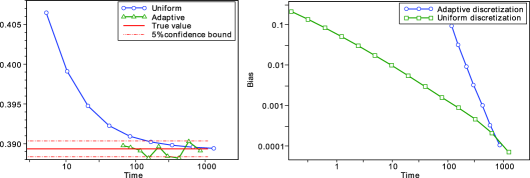
Figure 1: Illustration for Example 1. Left: values returned by the uniform discretization algorithm and the adaptive algorithm, as function of the computational time for $10^{6}$ paths, measured in seconds. Different points on the graph correspond to different numbers of discretization dates for the uniform discretization (ranging from 32 to 8192) and different values of the tolerance parameter $\gamma$ for the adaptive algorithm (ranging from $7$ to $7\times 10^{-4}$). The curve for the uniform discretization is smooth because all the points have been generated using the same trajectories, while for the adaptive discretization different paths have been used. Right: comparison of the theoretical bias of the adaptive algorithm with the actual discretization bias of the uniform discretization.

The theoretical bias, computed as explained in Remark 4.1, is greater than the actual error, because the error estimates of Appendix C are upper bounds, and because it does not take into account the possible cancellation of errors on different intervals. Figure 1, right graph, compares the theoretical estimate of the bias of the adaptive algorithm with the actual bias of the uniform discretization. One can see that for small computational times, the theoretical bias for the adaptive algorithm is greater than the error of the uniform discretization, however, the theoretical bias converges to zero much faster, and for relatively large computational times is actually smaller than the error of the uniform discretization. The empirical convergence rate (estimated from the slope of the straight lines) is $T^{-0.81}$ for the uniform discretization and $T^{-3.4}$ for the theoretical bias of the adaptive algorithm.

Example 2.

In our second example, we evaluate the probability $\mathbb{P}[\sup_{0\leq s\leq 1}X_{s}\leq 10^{-2}]$, which again can be expressed in terms of the function (33) by taking $T=1$, $F(X_{1})=1$, and the domain $(a,b)=(-\infty,10^{-2})$. In contrast to Example 1, here we consider a situation where the starting point is close to the boundary. In this case, as we shall see below, the advantage of the adaptive algorithm is more striking, since the process can cross the boundary and come back while it is still close to the starting point and, hence, a very fine discretization will be necessary to detect this event with uniformly spaced observations. As a result, for the uniform discretization we do not observe convergence to a sufficient precision even with 16 384 points, and therefore the true value cannot be estimated as in the previous example. Instead, we shall use as the true value the value produced by the adaptive algorithm with $10^{7}$ Monte Carlo paths and equal to $0.0360$, with standard deviation of $6\times 10^{-5}$ and theoretical bias of $3\times 10^{-5}$.

Similarly to the previous example, Figure 2 shows the dependence of the values computed by the two algorithms on the computational time required for $10^{6}$ MC trajectories. Here, the adaptive algorithm exhibits the same kind of behavior as in the Example 1 above: all the points generated by the algorithm are within the confidence bounds of the true value. However, for the uniform discretization, the convergence is much slower than before and only the last value obtained with 16384 discretization points falls within the confidence bounds. Figure 2, right graph, compares the theoretical estimate of the bias of the adaptive algorithm with the actual bias of the uniform discretization. Once again, the behavior of the adaptive algorithm is roughly the same as in the previous example, showing that the method is robust with respect to the parameters on the problem. On the other hand, as expected, the uniform discretization presents a significant bias in this case (the convergence rates are similar to those obtained in the previous example, but the constant for the uniform discretization is much bigger).

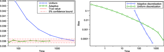
Figure 2: Illustration for Example 2. Left: values returned by the uniform discretization algorithm and the adaptive algorithm, as function of the computational time for $10^{6}$ paths, measured in seconds. Different points on the graph correspond to different numbers of discretization dates for the uniform discretization (ranging from 256 to 16384) and different values of the tolerance parameter $\gamma$ for the adaptive algorithm (ranging from $9$ to $9\times 10^{-3}$). Right: comparison of the theoretical bias of the adaptive algorithm with the actual discretization bias of the uniform discretization.

Appendix A Proofs of Section 2

A.1 Proof of Theorem 2.1

Throughout the proof, we shall use the notation

$${\bar{Y}_{t}:=\sup_{0\leq s\leq t}Y_{s}\quad\mbox{and}\quad\underline{Y}_{t}:=\inf_{0\leq s\leq t}Y_{s}}$$ (48)

for a given cádlág process $(Y_{t})_{t\geq 0}$. Without loss of generality (by considering separately the positive and the negative part), we can and will assume that $\varphi$ is nonnegative. Additionally, assume that $a\in(-\infty,0)$ and $b\in(0,\infty)$. The cases $a=-\infty$ and $b=\infty$ will be evident from the proof below. We also let $\|\varphi\|_{\infty}:=\operatorname{ess\,sup}_{x}\varphi(x)$, $\|\varphi\|_{\mathrm{Lip}}$ be the Lipschitz norm of $\varphi$, $I_{\delta}(y):=({y-\delta},y+\delta)$, $\eta:=\delta_{0}/2$, $c=b\wedge|a|$, $B:=\{\tau\leq t\}=\{\bar{X}_{t}\geq b\mbox{ or }\underline{X}_{t}\leq a\}$, $U_{t}^{\varepsilon}:=\sup_{s\leq t}|X^{\varepsilon}_{s}|$, and $a_{\varepsilon}:=\sup_{x}s_{\varepsilon}(x)$, which are finite in light of (10). In what follows, $\mathcal{F}_{t}^{\varepsilon}:=\sigma(X^{\varepsilon}_{s}\colon\ s\leq t)\vee\mathcal{N}$ where $\mathcal{N}$ denotes the null sets of $\mathcal{F}$. To lighten the notation below, whenever the $\operatorname{ess\,sup}$ of a function $g$, defined $\mathcal{L}$-a.e. in some region, is considered, we shall simply write $\sup_{u}g(u)$ instead of $\operatorname{ess\,sup}_{u}g(u)$.

The idea is to condition on the number of jumps of the compound Poisson component $Z^{\varepsilon}$. To this end, let us denote

$$A_{k}(t) = \mathbb{E}\bigl{(}\varphi(X_{\tau}){\mathbf{1}}_{\{\tau\leq t,X_{t}\in I_{\delta}(y),N_{t}^{\varepsilon}=k\}}\bigr{)}\qquad\mbox{for }k=0,1,2,$$

$$A_{3}(t) = \mathbb{E}\bigl{(}\varphi(X_{\tau}){\mathbf{1}}_{\{\tau\leq t,X_{t}\in I_{\delta}(y),N_{t}^{\varepsilon}\geq 3\}}\bigr{)},$$

so that clearly

$$\mathbb{E}\bigl{(}\varphi(X_{\tau})\mathbf{1}_{\{\tau\leq t,X_{t}\in I_{\delta}(y)\}}\bigr{)}=A_{0}(t)+\cdots+A_{3}(t).$$ (49)

Note that each of the terms on the right-hand side of the previous equation can be expressed as

$$A_{k}(t)=\int_{y-\delta}^{y+\delta}P_{t}^{k}(u)\,\mathrm{d}u\qquad(k=0,\ldots,3)$$ (50)

for some nonnegative functions $P^{k}_{t}(u)$. Indeed, for $k=0,1,2$, by the standard definition of conditional expectation,

$$A_{k}(t) = \mathbb{E}\bigl{(}\varphi(X_{\tau}){\mathbf{1}}_{\{\tau\leq t,X_{t}\in I_{\delta}(y),N_{t}^{\varepsilon}=k\}}\bigr{)}=\mathbb{E}\bigl{(}\mathbb{E}\bigl{(}\varphi(X_{\tau}){\mathbf{1}}_{\{\tau\leq t,N_{t}^{\varepsilon}=k\}}|X_{t}\bigr{)}\mathbf{1}_{\{X_{t}\in I_{\delta}(y)\}}\bigr{)}$$

$$= \int_{{y-\delta}}^{y+\delta}\mathbb{E}\bigl{(}\varphi(X_{\tau})\mathbf{1}_{\{\tau\leq t,N_{t}^{\varepsilon}=k\}}|X_{t}=u\bigr{)}f_{t}(u)\,\mathrm{d}u=:\int_{{y-\delta}}^{y+\delta}P_{t}^{k}(u)\,\mathrm{d}u.$$

The case $k=3$ is treated in the same way. Let us analyze each of the four terms in the right-hand side of (49).

(1) No big jump. Note that, on the event $N_{t}^{\varepsilon}=0$, $X_{s}=X_{s}^{\varepsilon}$ for all $s\leq t$ and, thus, $\{\tau\leq t\}=\{\tau^{\varepsilon}\leq t\}$, where $\tau^{\varepsilon}:=\inf\{u\geq 0\colon\ X_{u}^{\varepsilon}\notin(a,b)\}$. Therefore,

$$A_{0}(t) = \mathbb{E}\bigl{(}\varphi\bigl{(}X_{\tau^{\varepsilon}}^{\varepsilon}\bigr{)}\mathbf{1}_{\{\tau^{\varepsilon}\leq t,X^{\varepsilon}_{t}\in I_{\delta}(y),N_{t}^{\varepsilon}=0\}}\bigr{)}$$

$$= \mathbb{E}\bigl{(}\varphi\bigl{(}X_{\tau^{\varepsilon}}^{\varepsilon}\bigr{)}\mathbf{1}_{\{\tau^{\varepsilon}\leq t,X^{\varepsilon}_{t}\in I_{\delta}(y)\}}\bigr{)}\mathbb{P}\bigl{(}N_{t}^{\varepsilon}=0\bigr{)},$$

where in the last equality we used the independence of $X^{\varepsilon}$ and $N^{\varepsilon}$. Next, conditioning on $\mathcal{F}_{\tau^{\varepsilon}}^{\varepsilon}$, it follows that

$$A_{0}(t)=\mathrm{e}^{-\lambda_{\varepsilon}t}\mathbb{E}\bigl{(}\varphi\bigl{(}X_{\tau^{\varepsilon}}^{\varepsilon}\bigr{)}\mathbf{1}_{\{\tau^{\varepsilon}\leq t,X_{t}^{\varepsilon}\in I_{\delta}(y)\}}\bigr{)}=\mathrm{e}^{-\lambda_{\varepsilon}t}\mathbb{E}\bigl{(}\mathbb{E}\bigl{(}\mathbf{1}_{\{X_{t}^{\varepsilon}\in I_{\delta}(y)\}}|\mathcal{F}_{\tau^{\varepsilon}}^{\varepsilon}\bigr{)}\varphi\bigl{(}X_{\tau^{\varepsilon}}^{\varepsilon}\bigr{)}\mathbf{1}_{\{\tau^{\varepsilon}\leq t\}}\bigr{)}.$$

By Markov’s property,

$$A_{0}(t) = \mathrm{e}^{-\lambda_{\varepsilon}t}\mathbb{E}\bigl{(}\mathbb{E}\bigl{(}{\mathbf{1}}_{\{X_{t}^{\varepsilon}-X_{\tau^{\varepsilon}}^{\varepsilon}+X_{\tau^{\varepsilon}}^{\varepsilon}\in I_{\delta}(y)\}}|\mathcal{F}^{\varepsilon}_{\tau^{\varepsilon}}\bigr{)}\varphi\bigl{(}X_{\tau^{\varepsilon}}^{\varepsilon}\bigr{)}\mathbf{1}_{\{\tau^{\varepsilon}\leq t\}}\bigr{)}$$

$$= {\mathrm{e}^{-\lambda_{\varepsilon}t}}\mathbb{E}\bigl{(}F\bigl{(}X_{\tau^{\varepsilon}}^{\varepsilon},t-\tau^{\varepsilon}\bigr{)}\varphi\bigl{(}X_{\tau^{\varepsilon}}^{\varepsilon}\bigr{)}\mathbf{1}_{\{\tau^{\varepsilon}\leq t\}}\bigr{)},$$

where $F(z,s)=\mathbb{P}(z+X_{s}^{\varepsilon}\in I_{\delta}(y))$. Note that if $\tau^{\varepsilon}=t$, then $F(X_{\tau^{\varepsilon}}^{\varepsilon},t-\tau^{\varepsilon})=0$ since $X_{\tau^{\varepsilon}}^{\varepsilon}\in(a,b)^{c}$ and $I_{\delta}(y)\subset(a,b)$. On the other hand, on the event $\tau^{\varepsilon}<t$,

$$F\bigl{(}X_{\tau^{\varepsilon}}^{\varepsilon},t-\tau^{\varepsilon}\bigr{)}=\int_{{y-\delta}}^{y+\delta}f_{t-\tau^{\varepsilon}}^{\varepsilon}\bigl{(}u-X_{\tau^{\varepsilon}}^{\varepsilon}\bigr{)}\,\mathrm{d}u\leq\int_{y-\delta}^{y+\delta}\sup_{0<s\leq t}\sup_{x\in(a,b)^{c}}f_{s}^{\varepsilon}(u-x)\,\mathrm{d}u,$$

since again $X_{\tau^{\varepsilon}}^{\varepsilon}\in(a,b)^{c}$. Putting the two previous cases together and recalling (50), we have

$$A_{0}(t)=\int_{y-\delta}^{y+\delta}P_{t}^{0}(u)\,\mathrm{d}u \leq \int_{y-\delta}^{y+\delta}\Bigl{(}\mathrm{e}^{-\lambda_{\varepsilon}t}\|\varphi\|_{\infty}\sup_{0<s\leq t}\sup_{x\in(a,b)^{c}}f_{s}^{\varepsilon}(u-x)\Bigr{)}\,\mathrm{d}u$$

$$=: \int_{y-\delta}^{y+\delta}\bar{P}^{0}_{t}(u)\,\mathrm{d}u,$$

implying that $P^{0}_{t}(u)\leq\bar{P}_{t}^{0}(u)$, for $\mathcal{L}$-a.e. $u\in(a+\delta_{0},b-\delta_{0})$. Furthermore, using (13)(ii),

$$\sup_{{a+\delta_{0}<u<b-\delta_{0}}}P_{t}^{0}(u)\leq\sup_{{a+\delta_{0}<u<b-\delta_{0}}}\bar{P}_{t}^{0}(u)\leq\|\varphi\|_{\infty}c_{3}(\delta_{0},\varepsilon)t^{3}\qquad(t<t_{0}).$$

(2) One big jump. Let $\tau_{i}$ and $Y_{i}$ be the time and size of the $i$th jump of $Z^{\varepsilon}$. Clearly, on the event $\{N_{t}^{\varepsilon}=1\}$,

$$\varphi(X_{\tau})\mathbf{1}_{\{\tau\leq t,X_{t}\in I_{\delta}(y),{N_{t}^{\varepsilon}=1}\}} = \varphi\bigl{(}X_{\tau}^{\varepsilon}\bigr{)}\mathbf{1}_{\{\tau<\tau_{1},X_{t}^{\varepsilon}+Y_{1}\in I_{\delta}(y),{N_{t}^{\varepsilon}=1}\}}$$

$${}+\varphi\bigl{(}X_{\tau}^{\varepsilon}+Y_{1}\bigr{)}{\mathbf{1}}_{\{\tau_{1}\leq\tau\leq t,X_{t}^{\varepsilon}+Y_{1}\in I_{\delta}(y),{N_{t}^{\varepsilon}=1}\}}$$

$$\leq \|\varphi\|_{\infty}\mathbf{1}_{\{X_{t}^{\varepsilon}+Y_{1}\in I_{\delta}(y),{N_{t}^{\varepsilon}=1}\}}\mathbf{1}_{\{\bar{X}^{\varepsilon}_{t}\geq b\ \mathrm{or}\ \underline{X}_{t}^{\varepsilon}\leq a\}}$$

$${}+\|\varphi\|_{\infty}\mathbf{1}_{\{X_{t}^{\varepsilon}+Y_{1}\in I_{\delta}(y),{N_{t}^{\varepsilon}=1}\}}{\mathbf{1}_{\{\bar{X}^{\varepsilon}_{t}+Y_{1}\geq b\ \mathrm{or}\ \underline{X}_{t}^{\varepsilon}+Y_{1}\leq a\}}}.$$

It follows that

$$0\leq A_{1}(t) \leq \|\varphi\|_{\infty}\mathbb{E}({\mathbf{1}}_{\{U_{t}^{\varepsilon}\geq c,X_{t}^{\varepsilon}+Y_{1}\in I_{\delta}(y),N_{t}^{\varepsilon}=1\}})$$

$${}+\|\varphi\|_{\infty}\mathbb{E}(\mathbf{1}_{\{Y_{1}\geq b-\bar{X}_{t}^{\varepsilon}\ \mathrm{or}\ Y_{1}\leq a-\underline{X}^{\varepsilon}_{t}\}}{\mathbf{1}}_{\{X_{t}^{\varepsilon}+Y_{1}\in I_{\delta}(y),N_{t}^{\varepsilon}=1\}})$$

$$= \underbrace{\mathrm{e}^{-\lambda_{\varepsilon}t}\|\varphi\|_{\infty}\lambda_{\varepsilon}t\mathbb{E}(\mathbf{1}_{\{U_{t}^{\varepsilon}\geq c,X_{t}^{\varepsilon}+Y_{1}\in I_{\delta}(y)\}})}_{A_{1,1}(t)}$$

$${}+\underbrace{{\mathrm{e}^{-\lambda_{\varepsilon}t}\|\varphi\|_{\infty}\lambda_{\varepsilon}t\mathbb{E}(\mathbf{1}_{\{Y_{1}\geq b-\bar{X}_{t}^{\varepsilon}\ \mathrm{or}\ Y_{1}\leq a-\underline{X}^{\varepsilon}_{t}\}}\mathbf{1}_{\{X_{t}^{\varepsilon}+Y_{1}\in I_{\delta}(y)\}})}}_{A_{1,2}(t)},$$

where in the last equality we use the joint independence of $N^{\varepsilon}$, $Y_{1}$, and $X^{\varepsilon}$. Conditioning on $\sigma(X_{s}^{\varepsilon}\colon\ s\geq 0)$ and applying Fubini,

$$A_{1,1}(t) = {\mathrm{e}^{-\lambda_{\varepsilon}t}}\|\varphi\|_{\infty}t\mathbb{E}\biggl{(}\mathbf{1}_{\{{U}_{t}^{\varepsilon}\geq c\}}\int_{{y-\delta}-X_{t}^{\varepsilon}}^{y+\delta-X_{t}^{\varepsilon}}s_{\varepsilon}(v)\,\mathrm{d}v\biggr{)}$$

$$= \int_{{y-\delta}}^{y+\delta}\underbrace{{\mathrm{e}^{-\lambda_{\varepsilon}t}}\|\varphi\|_{\infty}t\mathbb{E}\bigl{(}\mathbf{1}_{\{{U}_{t}^{\varepsilon}\geq c\}}s_{\varepsilon}\bigl{(}u-X_{t}^{\varepsilon}\bigr{)}\bigr{)}}_{\bar{P}_{t}^{1,1}(u)}\,\mathrm{d}u.$$

Using (10) and Lemma 2.1, $\sup_{u}\bar{P}_{t}^{1,1}(u)\leq{\mathrm{e}^{-\lambda_{\varepsilon}t}}t\|\varphi\|_{\infty}a_{\varepsilon}\mathbb{P}({U}_{t}^{\varepsilon}\geq c)\leq\mathrm{e}^{-\lambda_{\varepsilon}t}a_{\varepsilon}\|\varphi\|_{\infty}\times C_{2}(c,\varepsilon)t^{3},$ where $\varepsilon>0$ is chosen small enough. Similarly, conditioning on $\sigma(X_{s}^{\varepsilon}\colon\ s\geq 0)$, making the substitution $u=X_{t}^{\varepsilon}+v$, and applying Fubini,

$$A_{1,2}(t) = {\mathrm{e}^{-\lambda_{\varepsilon}t}}\|\varphi\|_{\infty}t\mathbb{E}\biggl{(}\int\mathbf{1}_{\{v\leq a-\underline{X}^{\varepsilon}_{t}\ \mathrm{or}\ v\geq b-\bar{X}_{t}^{\varepsilon}\}}\mathbf{1}_{\{{y-\delta}<X_{t}^{\varepsilon}+v\leq y+\delta\}}s_{\varepsilon}(v)\,\mathrm{d}v\biggr{)}$$

$$= \int_{{y-\delta}}^{y+\delta}\underbrace{{\mathrm{e}^{-\lambda_{\varepsilon}t}}\|\varphi\|_{\infty}t\mathbb{E}\bigl{(}\mathbf{1}_{\{u\leq a+X_{t}^{\varepsilon}-\underline{X}^{\varepsilon}_{t}\ \mathrm{or}\ u\geq b+X_{t}^{\varepsilon}-\bar{X}_{t}^{\varepsilon}\}}s_{\varepsilon}\bigl{(}u-X_{t}^{\varepsilon}\bigr{)}\bigr{)}}_{\bar{P}_{t}^{1,2}(u)}\,\mathrm{d}u.$$

Using again Lemma 2.1,

$$\sup_{u\in(a+\delta_{0},b-\delta_{0})}\bar{P}_{t}^{1,2}(u) \leq {\mathrm{e}^{-\lambda_{\varepsilon}t}}\|\varphi\|_{\infty}ta_{\varepsilon}\mathbb{P}\bigl{(}{X}_{t}^{\varepsilon}-\underline{X}_{t}^{\varepsilon}\geq\delta_{0}\ \mathrm{or}\ \bar{X}_{t}^{\varepsilon}-X_{t}^{\varepsilon}\geq\delta_{0}\bigr{)}$$

$$\leq {\mathrm{e}^{-\lambda_{\varepsilon}t}}\|\varphi\|_{\infty}ta_{\varepsilon}\mathbb{P}\bigl{(}\bar{X}_{t}^{\varepsilon}-\underline{X}_{t}^{\varepsilon}\geq\delta_{0}\bigr{)}$$

$$\leq {\mathrm{e}^{-\lambda_{\varepsilon}t}}\|\varphi\|_{\infty}ta_{\varepsilon}\mathbb{P}\Bigl{(}\sup_{s\leq t}\bigl{|}{X}_{s}^{\varepsilon}\bigr{|}\geq\delta_{0}/2\Bigr{)}$$

$$\leq {\mathrm{e}^{-\lambda_{\varepsilon}t}}\|\varphi\|_{\infty}a_{\varepsilon}C_{2}(\delta_{0}/2,\varepsilon)t^{3}.$$

Therefore, recalling from (50), the nonnegative function $P_{t}^{1}(u)$ is such that,for $\mathcal{L}$-a.e. $u\in(a+\delta_{0},b-\delta_{0})$, $0\leq P_{t}^{1}(u)\leq\sum_{\ell=1}^{2}\bar{P}_{t}^{1,\ell}(u)\leq\|\varphi\|_{\infty}a_{\varepsilon}t^{3}(C_{2}(c,\varepsilon)+C_{2}(\eta,\varepsilon))$.

(3) Two big jumps. As before, let $\tau_{i}$ and $Y_{i}$ be the time and size of the $i$th jump of $Z^{\varepsilon}$. Clearly,

$$\varphi(X_{\tau})\mathbf{1}_{\{\tau\leq t,X_{t}\in I_{\delta}(y),{N_{t}^{\varepsilon}=2}\}} = \varphi\bigl{(}X_{\tau}^{\varepsilon}\bigr{)}\mathbf{1}_{\{\tau<\tau_{1},X_{t}^{\varepsilon}+Y_{1}+Y_{2}\in I_{\delta}(y),{N_{t}^{\varepsilon}=2}\}}$$

$${}+\varphi\bigl{(}X_{\tau}^{\varepsilon}+Y_{1}\bigr{)}{\mathbf{1}}_{\{\tau_{1}\leq\tau<\tau_{2},X_{t}^{\varepsilon}+Y_{1}+Y_{2}\in I_{\delta}(y),{N_{t}^{\varepsilon}=2}\}}$$

$${}+\varphi\bigl{(}X_{\tau}^{\varepsilon}+Y_{1}+Y_{2}\bigr{)}\mathbf{1}_{\{\tau_{2}\leq\tau\leq t,X_{t}^{\varepsilon}+Y_{1}+Y_{2}\in I_{\delta}(y),{N_{t}^{\varepsilon}=2}\}}$$

$$\leq {\|\varphi\|_{\infty}}{\mathbf{1}}_{\{\exists s<\tau_{1}\colon\ X^{\varepsilon}_{s}\notin(a,b);X_{t}^{\varepsilon}+Y_{1}+Y_{2}\in I_{\delta}(y);{N_{t}^{\varepsilon}=2}\}}$$

$${}+{\varphi\bigl{(}X^{\varepsilon}_{\tau}+Y_{1}\bigr{)}{{\mathbf{1}}}_{\{\exists s\in[\tau_{1},\tau_{2})\colon\ X^{\varepsilon}_{s}+Y_{1}\notin(a,b);X_{t}^{\varepsilon}+Y_{1}+Y_{2}\in I_{\delta}(y);{N_{t}^{\varepsilon}=2}\}}}$$

$${}+{\|\varphi\|_{\infty}}{\mathbf{1}}_{\{\exists s\in[\tau_{2},t]\colon\ X^{\varepsilon}_{s}+Y_{1}+Y_{2}\notin(a,b);X_{t}^{\varepsilon}+Y_{1}+Y_{2}\in I_{\delta}(y);{N_{t}^{\varepsilon}=2}\}}.$$

Then, using the independence of $N^{\varepsilon}$, the $Y_{i}$’s, and $X^{\varepsilon}$ in the first and last terms, we have the inequality:

$$A_{2}(t) \leq {\mathrm{e}^{-\lambda_{\varepsilon}t}}\bigl{(}t^{2}/2\bigr{)}\lambda_{\varepsilon}^{2}\|\varphi\|_{\infty}\mathbb{E}({\mathbf{1}}_{\{{U}_{t}^{\varepsilon}\geq c,X_{t}^{\varepsilon}+Y_{1}+Y_{2}\in I_{\delta}(y)\}})$$

$${}+\mathbb{E}\bigl{(}\varphi\bigl{(}{X}_{\tau}^{\varepsilon}+Y_{1}\bigr{)}\mathbf{1}_{\{\bar{X}^{\varepsilon}_{t}+Y_{1}\geq b\ \mathrm{or}\ \underline{X}_{t}^{\varepsilon}+Y_{1}\leq a;X_{t}^{\varepsilon}+Y_{1}+Y_{2}\in I_{\delta}(y);{N_{t}^{\varepsilon}=2}\}}\bigr{)}$$

$${}+{\mathrm{e}^{-\lambda_{\varepsilon}t}}{\bigl{(}t^{2}/2\bigr{)}\lambda_{\varepsilon}^{2}\|\varphi\|_{\infty}\mathbb{E}(\mathbf{1}_{\{\bar{X}^{\varepsilon}_{t}+Y_{1}+Y_{2}\geq b\ \mathrm{or}\ \underline{X}^{\varepsilon}_{t}+Y_{1}+Y_{2}\leq a;X_{t}^{\varepsilon}+Y_{1}+Y_{2}\in I_{\delta}(y)\}})},\qquad$$

$$=: {A_{2,1}(t)+A_{2,2}(t)+A_{2,3}(t).}$$

As before, conditioning on $\sigma(X_{s}^{\varepsilon}\colon\ s\geq 0)$, changing variable from $w$ to $u=X_{t}^{\varepsilon}+v+w$, and applying Fubini,

$$A_{2,1}(t) = {\mathrm{e}^{-\lambda_{\varepsilon}t}}2^{-1}\|\varphi\|_{\infty}t^{2}\mathbb{E}\biggl{(}\int\!\!\!\int\mathbf{1}_{\{U_{t}^{\varepsilon}\geq c\}}{\mathbf{1}}_{\{{y-\delta}<X_{t}^{\varepsilon}+w+v<y+\delta\}}s_{\varepsilon}(v)s_{\varepsilon}(w)\,\mathrm{d}v\,\mathrm{d}w\biggr{)}$$

$$= \int_{{y-\delta}}^{y+\delta}{\mathrm{e}^{-\lambda_{\varepsilon}t}}2^{-1}\|\varphi\|_{\infty}t^{2}\int_{-\infty}^{\infty}s_{\varepsilon}(v)\mathbb{E}\bigl{(}\mathbf{1}_{\{U^{\varepsilon}_{t}\geq c\}}s_{\varepsilon}\bigl{(}u-X_{t}^{\varepsilon}-v\bigr{)}\bigr{)}\,\mathrm{d}v\,\mathrm{d}u$$

$$=: {\int_{{y-\delta}}^{y+\delta}\bar{P}_{t}^{2,1}(u)\,\mathrm{d}u},$$

and, hence,

$$\sup_{u}\bar{P}_{t}^{2,1}(u) \leq{\mathrm{e}^{-\lambda_{\varepsilon}t}}2^{-1}\|\varphi\|_{\infty}t^{2}\lambda_{\varepsilon}a_{\varepsilon}\mathbb{P}\bigl{(}U_{t}^{\varepsilon}\geq c\bigr{)}\leq{\mathrm{e}^{-\lambda_{\varepsilon}t}}2^{-1}\|\varphi\|_{\infty}\lambda_{\varepsilon}a_{\varepsilon}C_{1}(c,\varepsilon)t^{3}.$$

Similarly, $A_{2,3}(t)$ can be written as

$${\mathrm{e}^{-\lambda_{\varepsilon}t}}2^{-1}\|\varphi\|_{\infty}t^{2}\mathbb{E}\biggl{(}\int\!\!\!\int\mathbf{1}_{\{\bar{X}^{\varepsilon}_{t}+v+w\geq b\ \mathrm{or}\ \underline{X}^{\varepsilon}_{t}+v+w\leq a\}}\mathbf{1}_{\{{y-\delta}<X_{t}^{\varepsilon}+w+v<y+\delta\}}s_{\varepsilon}(v)s_{\varepsilon}(w)\,\mathrm{d}v\,\mathrm{d}w\biggr{)}$$

$$\quad=\int_{{y-\delta}}^{y+\delta}{\mathrm{e}^{-\lambda_{\varepsilon}t}}2^{-1}\|\varphi\|_{\infty}t^{2}$$

(58)

$$\hskip 22.0pt\qquad{}\times\int\mathbb{E}\bigl{(}\mathbf{1}_{\{\bar{X}^{\varepsilon}_{t}-X_{t}^{\varepsilon}+u\geq b\ \mathrm{or}\ \underline{X}^{\varepsilon}_{t}-X_{t}^{\varepsilon}+u\leq a\}}s_{\varepsilon}\bigl{(}u-X_{t}^{\varepsilon}-v\bigr{)}\bigr{)}s_{\varepsilon}(v)\,\mathrm{d}v\,\mathrm{d}u$$

$$\quad=:{\int_{{y-\delta}}^{y+\delta}\bar{P}_{t}^{2,3}(u)\,\mathrm{d}u,}$$

and, thus, as in (A.1),

$$\sup_{u\in[a+\delta_{0},b-\delta_{0}]}\bar{P}_{t}^{2,3}(u) \leq {\mathrm{e}^{-\lambda_{\varepsilon}t}}2^{-1}\|\varphi\|_{\infty}t^{2}\lambda_{\varepsilon}a_{\varepsilon}\mathbb{P}\bigl{(}{X}_{t}^{\varepsilon}-\underline{X}_{t}^{\varepsilon}\geq\delta_{0}\ \mathrm{or}\ \bar{X}_{t}^{\varepsilon}-X_{t}^{\varepsilon}\geq\delta_{0}\bigr{)}$$

$$\leq {\mathrm{e}^{-\lambda_{\varepsilon}t}}2^{-1}\|\varphi\|_{\infty}\lambda_{\varepsilon}a_{\varepsilon}C_{1}(\delta_{0}/2,\varepsilon)t^{3}.$$

Finally, we provide an upper bound for $A_{2,2}(t)$. First, we use the bound $\varphi(X_{\tau}^{\varepsilon}+Y_{1})\leq\varphi(Y_{1})+\|\varphi\|_{\mathrm{Lip}}U_{t}^{\varepsilon}$ and again the independence of $N^{\varepsilon}$, the $Y_{i}$’s, and $X^{\varepsilon}$ to get

$$A_{2,2}(t)\leq\mathrm{e}^{-\lambda_{\varepsilon}t}\bigl{(}t^{2}/2\bigr{)}\lambda_{\varepsilon}^{2}\mathbb{E}\bigl{(}\bigl{\{}\varphi(Y_{1})+\|\varphi\|_{\mathrm{Lip}}U_{t}^{\varepsilon}\bigr{\}}{\mathbf{1}}_{\{\bar{X}^{\varepsilon}_{t}+Y_{1}\geq b\ \mathrm{or}\ \underline{X}_{t}^{\varepsilon}+Y_{1}\leq a;X_{t}^{\varepsilon}+Y_{1}+Y_{2}\in I_{\delta}(y)\}}\bigr{)}.$$

Next, by conditioning on $\sigma(X_{s}^{\varepsilon}\colon\ s\geq 0)\vee\sigma(Y_{1})$, we may write $A_{2,2}(t)$ as

$${\mathrm{e}^{-\lambda_{\varepsilon}t}}\bigl{(}t^{2}/2\bigr{)}\lambda_{\varepsilon}\mathbb{E}\biggl{(}\bigl{\{}\varphi(Y_{1})+\|\varphi\|_{\mathrm{Lip}}U_{t}^{\varepsilon}\bigr{\}}\mathbf{1}_{\{\bar{X}^{\varepsilon}_{t}+Y_{1}\geq b\ \mathrm{or}\ \underline{X}_{t}^{\varepsilon}+Y_{1}<a\}}\int_{{y-\delta}-X_{t}^{\varepsilon}-Y_{1}}^{y+\delta-X_{t}^{\varepsilon}-Y_{1}}s_{\varepsilon}(w)\,\mathrm{d}w\biggr{)}$$

$$\quad={\mathrm{e}^{-\lambda_{\varepsilon}t}}\bigl{(}t^{2}/2\bigr{)}\mathbb{E}\biggl{(}\int_{(a-\underline{X}_{t}^{\varepsilon},b-\bar{X}_{t}^{\varepsilon})^{c}}\bigl{\{}\varphi(v)+\|\varphi\|_{\mathrm{Lip}}U_{t}^{\varepsilon}\bigr{\}}s_{\varepsilon}(v)\int_{{y-\delta}-X_{t}^{\varepsilon}-v}^{y+\delta-X_{t}^{\varepsilon}-v}s_{\varepsilon}(w)\,\mathrm{d}w\,\mathrm{d}v\biggr{)}.$$

Next, changing variables and applying Fubini,

$$A_{2,2} = \int_{{y-\delta}}^{y+\delta}{{\mathrm{e}^{-\lambda_{\varepsilon}t}}2^{-1}t^{2}\mathbb{E}\biggl{(}\int_{(a-\underline{X}_{t}^{\varepsilon},b-\bar{X}_{t}^{\varepsilon})^{c}}\bigl{\{}\varphi(v)+\|\varphi\|_{\mathrm{Lip}}U_{t}^{\varepsilon}\bigr{\}}s_{\varepsilon}(v)s_{\varepsilon}\bigl{(}u-X_{t}^{\varepsilon}-v\bigr{)}\,\mathrm{d}v\biggr{)}}\,\mathrm{d}u$$

$$=: \int_{{y-\delta}}^{y+\delta}\bar{P}^{2,2}_{t}(u)\,\mathrm{d}u.$$

In order to find a lower bound for $A_{2}(t)$, note that

$$\varphi(X_{\tau})\mathbf{1}_{\{\tau\leq t,X_{t}\in I_{\delta}(y),{N_{t}^{\varepsilon}=2}\}}\geq\varphi\bigl{(}X_{\tau}^{\varepsilon}+Y_{1}\bigr{)}{\mathbf{1}}_{\{\tau_{1}\leq\tau<\tau_{2},X_{t}^{\varepsilon}+Y_{1}+Y_{2}\in I_{\delta}(y),{N_{t}^{\varepsilon}=2}\}}$$

$$\quad\geq\varphi\bigl{(}{X}_{\tau}^{\varepsilon}+Y_{1}\bigr{)}{\mathbf{1}}_{\{Y_{1}+\underline{X}^{\varepsilon}_{t}\geq b\ \mathrm{or}\ \bar{X}^{\varepsilon}_{t}+Y_{1}\leq a\}}\mathbf{1}_{\{\bar{X}^{\varepsilon}_{t}<b,\underline{X}^{\varepsilon}_{t}>a\}}\mathbf{1}_{\{X_{t}^{\varepsilon}+Y_{1}+Y_{2}\in I_{\delta}(y),{N_{t}^{\varepsilon}=2}\}}.$$

Using the previous inequality and the lower bound $\varphi(X_{\tau}^{\varepsilon}+Y_{1})\geq\varphi(Y_{1})-\|\varphi\|_{\mathrm{Lip}}U_{t}^{\varepsilon}$ together with the independence of $N^{\varepsilon}$, the $Y_{i}$’s, and $X^{\varepsilon}$, it follows that

$$A_{2}(t) \geq {\mathrm{e}^{-\lambda_{\varepsilon}t}}\frac{(\lambda_{\varepsilon}t)^{2}}{2}\mathbb{E}\bigl{(}\bigl{\{}\varphi(Y_{1})-\|\varphi\|_{\mathrm{Lip}}U_{t}^{\varepsilon}\bigr{\}}\mathbf{1}_{\{Y_{1}\in(a-\bar{X}^{\varepsilon}_{t},b-\underline{X}^{\varepsilon}_{t})^{c},\bar{X}^{\varepsilon}_{t}<b,\underline{X}^{\varepsilon}_{t}>a,X_{t}^{\varepsilon}+Y_{1}+Y_{2}\in I_{\delta}(y)\}}\bigr{)}$$

$$=: \int_{{y-\delta}}^{y+\delta}\underline{P}^{2}_{t}(u)\,\mathrm{d}u,$$

where $\underline{P}^{2}_{t}(u)$ is defined as

$${{\mathrm{e}^{-\lambda_{\varepsilon}t}}2^{-1}t^{2}\mathbb{E}\biggl{(}{\mathbf{1}}_{\{\bar{X}^{\varepsilon}_{t}<b,\underline{X}^{\varepsilon}_{t}>a\}}\int_{(a-\bar{X}_{t}^{\varepsilon},b-\underline{X}_{t}^{\varepsilon})^{c}}\bigl{\{}\varphi(v)-\|\varphi\|_{\mathrm{Lip}}U_{t}^{\varepsilon}\bigr{\}}s_{\varepsilon}(v)s_{\varepsilon}\bigl{(}u-X_{t}^{\varepsilon}-v\bigr{)}\,\mathrm{d}v\biggr{)}.}$$

As it will be proved in Lemma A.1 below, $\bar{P}_{t}^{2,2}(u)$ and $\underline{P}_{t}^{2}(u)$ are such that

$$\lim_{t\to 0}\sup_{u\in(a+\delta_{0},b-\delta_{0})}\biggl{|}\frac{1}{t^{2}}{\bar{P}_{t}^{2,2}(u)}-\frac{1}{2}\int_{(a,b)^{c}}\varphi(v)s_{\varepsilon}(v)s_{\varepsilon}(u-v)\,\mathrm{d}v\biggr{|} = 0,$$ (60)

$$\lim_{t\to 0}\sup_{u\in(a+\delta_{0},b-\delta_{0})}\biggl{|}\frac{1}{t^{2}}{\underline{P}_{t}^{2}(u)}-\frac{1}{2}\int_{(a,b)^{c}}\varphi(v)s_{\varepsilon}(v)s_{\varepsilon}(u-v)\,\mathrm{d}v\biggr{|} = 0.$$ (61)

Using (A.1), (61) and the corresponding bounds for $\bar{P}^{2,1}_{t}(u)$ and $\bar{P}^{2,3}_{t}(u)$, it follows that the nonnegative function $P_{t}^{2}(u)$ defined in (50) is such that

$${\lim_{t\to 0}}\sup_{u\in(a+\delta_{0},b-\delta_{0})}\biggl{|}\frac{1}{t^{2}}P_{t}^{2}(u)-\frac{1}{2}\int_{(a,b)^{c}}\varphi(v)s_{\varepsilon}(v)s_{\varepsilon}(u-v)\,\mathrm{d}v\biggr{|}=0.$$ (62)

(4) Three or more big jumps. As before, we have the following bound

$$0 \leq \mathbb{E}\bigl{(}\varphi(X_{\tau})\mathbf{1}_{\{\tau\leq t,X_{t}\in I_{\delta}(y),N_{t}^{\varepsilon}=n\}}\bigr{)}\leq\|\varphi\|_{\infty}\mathbb{E}(\mathbf{1}_{\{X^{\varepsilon}_{t}+\sum_{i=1}^{n}Y_{i}\in I_{\delta}(y),N_{t}^{\varepsilon}=n\}})$$

$$= \|\varphi\|_{\infty}\mathbb{P}\bigl{(}N_{t}^{\varepsilon}=n\bigr{)}\int_{{y-\delta}}^{y+\delta}\mathbb{E}\bigl{(}s^{*n}_{\varepsilon}\bigl{(}u-X_{t}^{\varepsilon}\bigr{)}\bigr{)}\,\mathrm{d}u.$$

Using the previous inequality and (50), we have

$$A_{3}(t)=\int_{{y-\delta}}^{y+\delta}P_{t}^{3}(u)\,\mathrm{d}u\leq\int_{{y-\delta}}^{y+\delta}\Biggl{[}\sum_{n=3}^{\infty}{\mathrm{e}^{-\lambda_{\varepsilon}t}}\frac{t^{n}}{n!}\|\varphi\|_{\infty}\mathbb{E}\bigl{(}s^{*n}_{\varepsilon}\bigl{(}u-X_{t}^{\varepsilon}\bigr{)}\bigr{)}\Biggr{]}\,\mathrm{d}u=:\int_{{y-\delta}}^{y+\delta}\bar{P}^{3}_{t}(u)\,\mathrm{d}u.$$

Since $\|s_{\varepsilon}^{*n}\|_{\infty}\leq\lambda^{n-1}_{\varepsilon}a_{\varepsilon}$,

$$\sup_{u}\bar{P}_{t}^{3}(u)\leq{\mathrm{e}^{-\lambda_{\varepsilon}t}}a_{\varepsilon}\|\varphi\|_{\infty}\sum_{n=3}^{\infty}\frac{t^{n}}{n!}\lambda_{\varepsilon}^{n-1}\leq C(\varepsilon)t^{3}$$ (63)

for some constant $C(\varepsilon)<\infty$, and we conclude that $0\leq P_{t}^{3}(u)\leq C(\varepsilon)t^{3}$ for $\mathcal{L}$-a.e. $u$.

Putting the four previous steps together, we conclude that $\mathbb{E}(\varphi(X_{\tau})\mathbf{1}_{\{\tau\leq t,X_{t}\in({y-\delta},y+\delta)\}})=\int_{{y-\delta}}^{y+\delta}P_{t}(u)\,\mathrm{d}u$, for a function $P_{t}(u)$ such that

$$\lim_{t\to 0}{\sup_{u\in(a+\delta_{0},b-\delta_{0})}}\biggl{|}\frac{1}{t^{2}}P_{t}(u)-\frac{1}{2}\int_{(a,b)^{c}}\varphi(v)s_{\varepsilon}(v)s_{\varepsilon}(u-v)\,\mathrm{d}v\biggr{|}=0.$$

Finally, it is easy to see that for any $u\in(a+\delta_{0},b-\delta_{0})$ and $a<0<b$, there exists an $\varepsilon_{0}>0$ small enough such that $\int_{(a,b)^{c}}\varphi(v)s_{\varepsilon}(v)s_{\varepsilon}(u-v)\,\mathrm{d}v=\int_{(a,b)^{c}}\varphi(v)s(v)s(u-v)\,\mathrm{d}v$, for all $0<{\varepsilon}<\varepsilon_{0}$. This concludes the proof. $\Box$

Lemma A.1.

Verification of (60) and (61).

Proof.

Let $0<\varepsilon<1$ and $M^{\varepsilon}_{t}:=X_{t}^{\varepsilon}-{\mu_{\varepsilon}}t$ be the martingale component of $X^{\varepsilon}$. We shall analyze the expressions appearing inside the absolute values on the right-hand side of equations (60) and (61). Define the random intervals ${{\bar{I}}:=(a-\underline{X}^{\varepsilon}_{t},b-\bar{X}_{t}^{\varepsilon})}$, $\underline{I}:=(a-\bar{X}_{t}^{\varepsilon},b-\underline{X}_{t}^{\varepsilon})$, and the corresponding limiting interval $J=(a,b)$, under the convention $(x,y)=\varnothing$ if $y<x$. Denote

$$D_{t}^{1}(u) = \mathbb{E}\biggl{(}\int_{\bar{I}^{c}}\bigl{\{}\varphi(v)+\|\varphi\|_{\mathrm{Lip}}U_{t}^{\varepsilon}\bigr{\}}s_{\varepsilon}(v)s_{\varepsilon}\bigl{(}u-X_{t}^{\varepsilon}-v\bigr{)}\,\mathrm{d}v\biggr{)}-\int_{J^{c}}\varphi(v)s_{\varepsilon}(v)s_{\varepsilon}(u-v)\,\mathrm{d}v,$$

$$D_{t}^{2}(u) = \mathbb{E}\biggl{(}\mathbf{1}_{\{\bar{X}_{t}^{\varepsilon}<b,\underline{X}_{t}^{\varepsilon}>a\}}\int_{\underline{I}^{c}}\bigl{\{}\varphi(v)-\|\varphi\|_{\mathrm{Lip}}U_{t}^{\varepsilon}\bigr{\}}s_{\varepsilon}(v)s_{\varepsilon}\bigl{(}u-X_{t}^{\varepsilon}-v\bigr{)}\,\mathrm{d}v\biggr{)}$$

$${}-\int_{J^{c}}\varphi(v)s_{\varepsilon}(v)s_{\varepsilon}(u-v)\,\mathrm{d}v.$$

Let us first analyze $D_{t}^{1}$. Clearly,

$$D_{t}^{1}(u) = {\|\varphi\|_{\mathrm{Lip}}\mathbb{E}\biggl{(}U_{t}^{\varepsilon}\int_{\bar{I}^{c}}s_{\varepsilon}(v)s_{\varepsilon}\bigl{(}u-X_{t}^{\varepsilon}-v\bigr{)}\,\mathrm{d}v\biggr{)}}$$

$${}+{\mathbb{E}\biggl{(}\int_{\bar{I}^{c}\setminus J^{c}}\varphi(v)s_{\varepsilon}(v)s_{\varepsilon}\bigl{(}u-X_{t}^{\varepsilon}-v\bigr{)}\,\mathrm{d}v\biggr{)}}$$

$${}+\mathbb{E}\biggl{(}\int_{J^{c}}\varphi(v)s_{\varepsilon}(v)\bigl{[}s_{\varepsilon}\bigl{(}u-X_{t}^{\varepsilon}-v\bigr{)}-s_{\varepsilon}(u-v)\bigr{]}\,\mathrm{d}v\biggr{)},$$

and, therefore, using that $\bar{I}^{c}\setminus J^{c}\subset(a,a-\underline{X}_{t}^{\varepsilon})\cup(b-\bar{X}_{t}^{\varepsilon},b)$, under the convention $(-\infty,-\infty)=(\infty,\infty)=\varnothing$,

$$\bigl{|}D_{t}^{1}(u)\bigr{|} \leq a_{\varepsilon}\lambda_{\varepsilon}\|\varphi\|_{\mathrm{Lip}}\mathbb{E}{U}_{t}^{\varepsilon}+a_{\varepsilon}^{2}\|\varphi\|_{\infty}\mathbb{E}\bigl{(}\bar{X}^{\varepsilon}_{t}-\underline{X}^{\varepsilon}_{t}\bigr{)}+\lambda_{\varepsilon}\|\varphi\|_{\infty}\bigl{\|}s^{\prime}_{\varepsilon}\bigr{\|}_{\infty}\mathbb{E}\bigl{|}X_{t}^{\varepsilon}\bigr{|}$$

$$\leq \bigl{(}a_{\varepsilon}\lambda_{\varepsilon}\|\varphi\|_{\mathrm{Lip}}+2\|\varphi\|_{\infty}a_{\varepsilon}^{2}\bigr{)}\Bigl{(}\mathbb{E}\sup_{s\leq t}\bigl{|}{M}_{s}^{\varepsilon}\bigr{|}+|{\mu_{\varepsilon}}|t\Bigr{)}+\|\varphi\|_{\infty}\lambda_{\varepsilon}\bigl{\|}s^{\prime}_{\varepsilon}\bigr{\|}_{\infty}\bigl{(}\mathbb{E}\bigl{|}M_{t}^{\varepsilon}\bigr{|}+|{\mu_{\varepsilon}}|t\bigr{)}.$$

Using the trivial inequalities $(\mathbb{E}\sup_{s\leq t}|{M}_{s}^{\varepsilon}|)^{2}\leq\mathbb{E}\sup_{s\leq t}({M}_{s}^{\varepsilon})^{2}$ and $(\mathbb{E}|{M}_{s}^{\varepsilon}|)^{2}\leq\mathbb{E}({M}_{s}^{\varepsilon})^{2}$, together with Doob’s inequality, we then get the bound

$$\bigl{|}D_{t}^{1}(u)\bigr{|} \leq \bigl{[}{2}a_{\varepsilon}\lambda_{\varepsilon}\|\varphi\|_{\mathrm{Lip}}+4\|\varphi\|_{\infty}a_{\varepsilon}^{2}+\|\varphi\|_{\infty}\lambda_{\varepsilon}\bigl{\|}s^{\prime}_{\varepsilon}\bigr{\|}_{\infty}\bigr{]}\sigma_{\varepsilon}t^{1/2}$$

$${}+\bigl{[}a_{\varepsilon}\lambda_{\varepsilon}\|\varphi\|_{\mathrm{Lip}}+2\|\varphi\|_{\infty}a_{\varepsilon}^{2}+\|\varphi\|_{\infty}\lambda_{\varepsilon}\bigl{\|}s^{\prime}_{\varepsilon}\bigr{\|}_{\infty}\bigr{]}|{\mu_{\varepsilon}}|t,$$

where $\sigma_{\varepsilon}^{2}:=\sigma^{2}+\int\bar{c}_{\varepsilon}(x)x^{2}\nu(\mathrm{d}x)$. For $D_{t}^{2}(u)$, note that

$$D_{t}^{2}(u) = -\mathbb{E}\biggl{(}\mathbf{1}_{\{\bar{X}_{t}^{\varepsilon}\geq b\ \mathrm{or}\ \underline{X}_{t}^{\varepsilon}\leq a\}}\int_{\underline{I}^{c}}\varphi(v)s_{\varepsilon}(v)s_{\varepsilon}\bigl{(}u-X_{t}^{\varepsilon}-v\bigr{)}\,\mathrm{d}v\biggr{)}$$

$${}+\|\varphi\|_{\mathrm{Lip}}\mathbb{E}\biggl{(}\mathbf{1}_{\{\bar{X}_{t}^{\varepsilon}<b,\underline{X}_{t}^{\varepsilon}>a\}}U_{t}^{\varepsilon}\int_{\underline{I}^{c}}s_{\varepsilon}(v)s_{\varepsilon}\bigl{(}u-X_{t}^{\varepsilon}-v\bigr{)}\,\mathrm{d}v\biggr{)}$$

$${}+\mathbb{E}\biggl{(}\int_{\underline{I}^{c}}\varphi(v)s_{\varepsilon}(v)s_{\varepsilon}\bigl{(}u-X_{t}^{\varepsilon}-v\bigr{)}\,\mathrm{d}v\biggr{)}-\int_{J^{c}}\varphi(v)s_{\varepsilon}(v)s_{\varepsilon}(u-v)\,\mathrm{d}v.$$

Defining $c=|a|\wedge b$ and following the same steps as above, it is easy to verify that $|D_{t}^{2}(u)|$ admits the following upper bound:

$${\bigl{|}D_{t}^{2}(u)\bigr{|}} \leq \|\varphi\|_{\infty}\lambda_{\varepsilon}a_{\varepsilon}\mathbb{P}\bigl{(}U^{\varepsilon}_{t}\geq c\bigr{)}+a_{\varepsilon}\lambda_{\varepsilon}\|\varphi\|_{\mathrm{Lip}}\mathbb{E}{U}_{t}^{\varepsilon}+2a_{\varepsilon}^{2}\|\varphi\|_{\infty}\mathbb{E}U_{t}^{\varepsilon}+\lambda_{\varepsilon}\|\varphi\|_{\infty}\bigl{\|}s^{\prime}_{\varepsilon}\bigr{\|}_{\infty}\mathbb{E}\bigl{|}X_{t}^{\varepsilon}\bigr{|}$$

$$\leq \|\varphi\|_{\infty}\lambda_{\varepsilon}a_{\varepsilon}C_{1}(c,\varepsilon)t+\bigl{[}2a_{\varepsilon}\lambda_{\varepsilon}\|\varphi\|_{\mathrm{Lip}}+4\|\varphi\|_{\infty}a_{\varepsilon}^{2}+\|\varphi\|_{\infty}\lambda_{\varepsilon}\bigl{\|}s^{\prime}_{\varepsilon}\bigr{\|}_{\infty}\bigr{]}\sigma_{\varepsilon}t^{1/2}$$

$${}+\bigl{[}a_{\varepsilon}\lambda_{\varepsilon}\|\varphi\|_{\mathrm{Lip}}+{2}\|\varphi\|_{\infty}a_{\varepsilon}^{2}+\|\varphi\|_{\infty}\lambda_{\varepsilon}\bigl{\|}s^{\prime}_{\varepsilon}\bigr{\|}_{\infty}\bigr{]}|{\mu_{\varepsilon}}|t,$$

where we had used the tail probability bound in (13). ∎

A.2 Proof of Proposition 1

We use the notation introduced at the beginning of Section A.1 above and, as before, we assume without loss of generality that $\varphi$ is nonnegative. As it was done in (49), by partitioning the space into the different values that $N_{t}^{\varepsilon}$ can take on, we can decompose $\mathbb{E}(\varphi(X_{\tau})\mathbf{1}_{\{X_{t}\in I_{\delta}(y)\}})$ into three terms: no big jumps, one big jump, and two or more big jumps. These terms can in turn be expressed as integrals of the form (50) using a procedure similar to (A.1). The term with no big jumps is such that

$$\int_{{y-\delta}}^{y+\delta}P_{t}^{0}(u)\,\mathrm{d}u := \mathbb{E}\bigl{(}\varphi(X_{\tau})\mathbf{1}_{\{X_{t}\in I_{\delta}(y),N_{t}^{\varepsilon}=0\}}\bigr{)}$$

$$\leq \|\varphi\|_{\infty}\mathbb{P}\bigl{(}X^{\varepsilon}_{t}\in I_{\delta}(y),N_{t}^{\varepsilon}=0\bigr{)}$$

$$= \int_{{y-\delta}}^{y+\delta}\mathrm{e}^{-\lambda_{\varepsilon}t}\|\varphi\|_{\infty}f^{\varepsilon}_{t}(u)\,\mathrm{d}u,$$

which yields an upper bound for $P_{t}^{0}(u)$ of the form $\bar{P}^{0}_{t}(u):=\mathrm{e}^{-\lambda_{\varepsilon}t}\|\varphi\|_{\infty}f^{\varepsilon}_{t}(u)$. Using (13)(ii), we can further upper bound $\bar{P}^{0}_{t}(u)$ by $\|\varphi\|_{\infty}c_{2}(c,\varepsilon)t^{2}$ uniformly in $(a-\delta_{0},b+\delta_{0})^{c}$. The term with two or more big jumps can be bounded similarly to the term with three or more big jumps in the previous section. Concretely, this term satisfies

$$\int_{{y-\delta}}^{y+\delta}P_{t}^{2}(u)\,\mathrm{d}u := \mathbb{E}\bigl{(}\varphi(X_{\tau})\mathbf{1}_{\{X_{t}\in I_{\delta}(y),N_{t}^{\varepsilon}\geq 2\}}\bigr{)}$$

$$\leq \int_{{y-\delta}}^{y+\delta}\Biggl{[}\sum_{n=2}^{\infty}{\mathrm{e}^{-\lambda_{\varepsilon}t}}\frac{t^{n}}{n!}\|\varphi\|_{\infty}\mathbb{E}\bigl{(}s^{*n}_{\varepsilon}\bigl{(}u-X_{t}^{\varepsilon}\bigr{)}\bigr{)}\Biggr{]}\,\mathrm{d}u=:\int_{{y-\delta}}^{y+\delta}\bar{P}^{2}_{t}(u)\,\mathrm{d}u,$$

and, using that $\|s_{\varepsilon}^{*n}\|_{\infty}\leq\lambda^{n-1}_{\varepsilon}a_{\varepsilon}$, we can further upper bound $\bar{P}^{2}_{t}(u)$ by $C(\varepsilon)t^{2}$ for a constant $C(\varepsilon)<\infty$. The term with exactly one jump is decomposed as follows:

$$\int_{{y-\delta}}^{y+\delta}P_{t}^{1}(u)\,\mathrm{d}u := \mathbb{E}\bigl{(}\varphi(X_{\tau})\mathbf{1}_{\{X_{t}\in I_{\delta}(y),N_{t}^{\varepsilon}=1\}}\bigr{)}$$

$$= \mathbb{E}\bigl{(}\varphi\bigl{(}X^{\varepsilon}_{\tau}\bigr{)}{\mathbf{1}}_{\{X_{t}\in I_{\delta}(y);\tau<\tau_{1};N_{t}^{\varepsilon}=1\}}\bigr{)}+\mathbb{E}\bigl{(}\varphi(X_{\tau}){\mathbf{1}}_{\{X_{t}\in I_{\delta}(y);\tau\geq\tau_{1};N_{t}^{\varepsilon}=1\}}\bigr{)},$$

where $\tau_{1}$ is the time of the first big jump. Out of these two terms, the first one satisfies

$$\mathbb{E}\bigl{(}\varphi\bigl{(}X^{\varepsilon}_{\tau}\bigr{)}{\mathbf{1}}_{\{X_{t}\in I_{\delta}(y);\tau<\tau_{1};N_{t}^{\varepsilon}=1\}}\bigr{)} \leq \|\varphi\|_{\infty}\mathbb{P}\bigl{[}\exists s\in[0,t]\colon\ X^{\varepsilon}_{s}\notin D;X^{\varepsilon}_{t}+Y_{1}\in I_{\delta};N_{t}^{\varepsilon}=1\bigr{]}$$

$$= \mathrm{e}^{-\lambda_{\varepsilon}t}\lambda_{\varepsilon}t\|\varphi\|_{\infty}\mathbb{P}\bigl{[}\exists s\in[0,t]\colon\ X^{\varepsilon}_{s}\notin D;X^{\varepsilon}_{t}+Y_{1}\in I_{\delta}\bigr{]}$$

$$\leq \int_{{y-\delta}}^{y+\delta}\mathrm{e}^{-\lambda_{\varepsilon}t}t\|\varphi\|_{\infty}\mathbb{E}\bigl{[}{\mathbf{1}}_{U^{\varepsilon}_{t}\geq c}s_{\varepsilon}\bigl{(}u-X_{t}^{\varepsilon}\bigr{)}\bigr{]}\,\mathrm{d}u,$$

where the integrand $\bar{P}^{1,1}_{t}(u):=\mathrm{e}^{-\lambda_{\varepsilon}t}t\|\varphi\|_{\infty}\mathbb{E}[{\mathbf{1}}_{U^{\varepsilon}_{t}\geq c}s_{\varepsilon}(u-X_{t}^{\varepsilon})]$ is uniformly bounded by $\|\varphi\|_{\infty}a_{\varepsilon}C_{1}(c,\varepsilon)t^{2}$. As for the second term

$$\mathbb{E}\bigl{(}\varphi(X_{\tau})\mathbf{1}_{\{X_{t}\in I_{\delta}(y);\tau\geq\tau_{1};N_{t}^{\varepsilon}=1\}}\bigr{)}=\mathbb{E}\bigl{(}\varphi\bigl{(}X^{\varepsilon}_{\tau}+Y_{1}\bigr{)}{\mathbf{1}}_{\{X_{t}^{\varepsilon}+Y_{1}\in I_{\delta}(y);\tau\geq\tau_{1};N_{t}^{\varepsilon}=1\}}\bigr{)},$$

it can be bounded from above by

$$\mathbb{E}\bigl{(}\varphi(Y_{1})\mathbf{1}_{\{X^{\varepsilon}_{t}+Y_{1}\in I_{\delta}(y);N_{t}^{\varepsilon}=1\}}\bigr{)}+\|\varphi\|_{\mathrm{Lip}}\mathbb{E}\bigl{(}U^{\varepsilon}_{t}{\mathbf{1}}_{\{X^{\varepsilon}_{t}+Y_{1}\in I_{\delta}(y);N_{t}^{\varepsilon}=1\}}\bigr{)}$$

$$\quad=\int_{{y-\delta}}^{y+\delta}\bigl{\{}\mathrm{e}^{-\lambda_{\varepsilon}t}t\mathbb{E}\bigl{[}\varphi\bigl{(}u-X_{t}^{\varepsilon}\bigr{)}s_{\varepsilon}\bigl{(}u-X_{t}^{\varepsilon}\bigr{)}\bigr{]}+\mathrm{e}^{-\lambda_{\varepsilon}t}t\|\varphi\|_{\mathrm{Lip}}\mathbb{E}\bigl{[}U^{\varepsilon}_{t}s_{\varepsilon}\bigl{(}u-X_{t}^{\varepsilon}\bigr{)}\bigr{]}\bigr{\}}\,\mathrm{d}u$$

$$\quad\leq\int_{{y-\delta}}^{y+\delta}\bigl{\{}t\varphi(u)s_{\varepsilon}(u)+t\bigl{(}\|\varphi\|_{\mathrm{Lip}}a_{\varepsilon}+\|\varphi\|_{\infty}\bigl{\|}s^{\prime}_{\varepsilon}\bigr{\|}_{\infty}\bigr{)}\mathbb{E}\bigl{[}\bigl{|}X^{\varepsilon}_{t}\bigr{|}\bigr{]}+t\|\varphi\|_{\mathrm{Lip}}a_{\varepsilon}\mathbb{E}\bigl{[}U^{\varepsilon}_{t}\bigr{]}\bigr{\}}\,\mathrm{d}u.$$

Similarly, this can be bounded from below by

$$\mathbb{E}\bigl{(}\varphi(Y_{1})\mathbf{1}_{\{X^{\varepsilon}_{t}+Y_{1}\in I_{\delta}(y);\bar{X}^{\varepsilon}_{t}<b;\underline{X}^{\varepsilon}_{t}>a;N_{t}^{\varepsilon}=1\}}\bigr{)}-\|\varphi\|_{\mathrm{Lip}}\mathbb{E}\bigl{(}U^{\varepsilon}_{t}{\mathbf{1}}_{\{X^{\varepsilon}_{t}+Y_{1}\in I_{\delta}(y);N_{t}^{\varepsilon}=1\}}\bigr{)}$$

$$\quad=\int_{y-\delta}^{y+\delta}\bigl{\{}\mathrm{e}^{-\lambda_{\varepsilon}t}t\mathbb{E}\bigl{(}\varphi\bigl{(}u-X_{t}^{\varepsilon}\bigr{)}s_{\varepsilon}\bigl{(}u-X_{t}^{\varepsilon}\bigr{)}\mathbf{1}_{\{\bar{X}^{\varepsilon}_{t}<b,\underline{X}^{\varepsilon}_{t}>a\}}\bigr{)}-\mathrm{e}^{-\lambda_{\varepsilon}t}t\|\varphi\|_{\mathrm{Lip}}\mathbb{E}\bigl{(}U^{\varepsilon}_{t}s_{\varepsilon}\bigl{(}u-X_{t}^{\varepsilon}\bigr{)}\bigr{)}\bigr{\}}\,\mathrm{d}u$$

$$\quad\geq\int_{y-\delta}^{y+\delta}\bigl{\{}t\varphi(u)s_{\varepsilon}(u)-\|\varphi\|_{\infty}a_{\varepsilon}\lambda_{\varepsilon}t^{2}-t\bigl{(}\|\varphi\|_{\mathrm{Lip}}a_{\varepsilon}+\|\varphi\|_{\infty}\bigl{\|}s^{\prime}_{\varepsilon}\bigr{\|}_{\infty}\bigr{)}\mathbb{E}\bigl{[}\bigl{|}X^{\varepsilon}_{t}\bigr{|}\bigr{]}$$

$$\hskip 24.0pt\qquad{}-t\|\varphi\|_{\mathrm{Lip}}a_{\varepsilon}\mathbb{E}\bigl{[}U^{\varepsilon}_{t}\bigr{]}-t\|\varphi\|_{\infty}a_{\varepsilon}C_{1}(c,\varepsilon)t\bigr{\}}\,\mathrm{d}u.$$

To conclude, we estimate $\mathbb{E}[|X^{\varepsilon}_{t}|]$ and $\mathbb{E}[U^{\varepsilon}_{t}]$ as in the proof of Lemma A.1 above.

Appendix B Proofs of Section 3

In this part, we provide the building blocks to develop an upper bound for the remainder $\mathcal{R}_{t}(u)$ appearing in (14).

B.1 Proof of Lemma 3.1

Let us first assume that ${\mu}\geq 0$ so that $X_{t}:=M_{t}+{\mu}t$ is a submartingale. By Doob’s inequality, for all $c>0$,

$$\mathbb{P}\Bigl{(}\sup_{s\leq t}{X_{s}}\geq\eta\Bigr{)}=\mathbb{P}\Bigl{(}\sup_{s\leq t}\mathrm{e}^{c{X_{s}}}\geq\mathrm{e}^{c\eta}\Bigr{)}\leq\frac{\mathbb{E}[\mathrm{e}^{c{X_{t}}}]}{\mathrm{e}^{c\eta}}=\mathrm{e}^{t\psi(c)-c\eta}$$ (66)

with $\psi(c)={{\mu}c}+\frac{\sigma^{2}c^{2}}{2}+\int_{|z|\leq\varepsilon}(\mathrm{e}^{cz}-1-cz)\nu(\mathrm{d}z)$. Minimizing the right-hand side over all $c>0$, we get, as in Rüschendorf and Woerner [38] (see page 87 therein),

$$\inf_{c>0}\mathrm{e}^{t\psi(c)-c\eta}=\exp\biggl{(}-t\int_{{\psi^{\prime}(0)}}^{\eta/t}\tau(z)\,\mathrm{d}z\biggr{)}=\exp\biggl{(}-t\int_{{{\mu}}}^{\eta/t}\tau(z)\,\mathrm{d}z\biggr{)},$$ (67)

where we are taking $t<\eta/{\mu}$ and ${\tau\mathchoice{\nobreak\,\colon}{\nobreak\,\colon}{\nobreak\,\colon\;}{\nobreak\,\colon\;}[0,\infty)\to\mathbb{R}}$ is the inverse function of

$$\psi^{\prime}(x)={\mu}+\sigma^{2}x+\int_{|z|\leq\varepsilon}z\bigl{(}\mathrm{e}^{zx}-1\bigr{)}\nu(\mathrm{d}z).$$ (68)

As in Houdré [25], note that, for $x\geq 0$,

$$0\leq\int_{|z|\leq\varepsilon}z\bigl{(}\mathrm{e}^{zx}-1\bigr{)}\nu(\mathrm{d}z) \leq \int_{|z|\leq\varepsilon}|z|\bigl{(}\mathrm{e}^{|z|x}-1\bigr{)}\nu(\mathrm{d}z)\leq\int_{|z|\leq\varepsilon}|z|\sum_{k=1}^{\infty}\frac{(|z|x)^{k}}{k!}\nu(\mathrm{d}z)$$

$$\leq \int_{|z|\leq\varepsilon}|z|^{2}\nu(\mathrm{d}z)\sum_{k=1}^{\infty}\frac{\varepsilon^{k-1}x^{k}}{k!}=\int_{|z|\leq\varepsilon}|z|^{2}\nu(\mathrm{d}z)\frac{1}{\varepsilon}\bigl{(}\mathrm{e}^{\varepsilon x}-1\bigr{)}.$$

From the previous inequality, for $x\geq 0$,

$$0\leq\psi^{\prime}(x)\leq{\mu}+\sigma^{2}x+\int_{|z|\leq\varepsilon}|z|^{2}\nu(\mathrm{d}z)\frac{1}{\varepsilon}\bigl{(}\mathrm{e}^{\varepsilon x}-1\bigr{)}\leq{\mu}+\frac{\mathrm{e}^{\varepsilon x}-1}{\varepsilon}\sigma_{\varepsilon}^{2},$$

where we used the fact that $\sigma^{2}_{\varepsilon}=\sigma^{2}+\int_{|z|\leq\varepsilon}|z|^{2}\nu(\mathrm{d}z)$. This implies that

$$\tau(z)\geq\frac{1}{\varepsilon}\log\biggl{\{}1+\frac{{z-{\mu}}}{\sigma_{\varepsilon}^{2}}\varepsilon\biggr{\}},$$

and therefore, substituting this into (66) and (67) and using that $v\ln(v)\leq(1+v)\ln(1+v)$ and $\mathrm{e}^{-v\log v}\leq\mathrm{e}^{\mathrm{e}^{-1}}$ for all $v>0$, we have

$$\mathbb{P}\Bigl{[}\sup_{s\leq t}{X_{s}}\geq\eta\Bigr{]} \leq \exp\biggl{\{}-\frac{t\sigma_{\varepsilon}^{2}}{\varepsilon^{2}}\int_{0}^{{\varepsilon{(\eta-{\mu}t)}}/{(t\sigma_{\varepsilon}^{2})}}\log(1+s)\,\mathrm{d}s\biggr{\}}$$

$$= \exp\biggl{\{}-\frac{t\sigma_{\varepsilon}^{2}}{\varepsilon^{2}}\biggl{(}\biggl{(}1+\frac{\varepsilon{(\eta-{\mu}t)}}{t\sigma_{\varepsilon}^{2}}\biggr{)}\log\biggl{(}1+\frac{\varepsilon{(\eta-{\mu}t)}}{t\sigma_{\varepsilon}^{2}}\biggr{)}-\frac{\varepsilon{(\eta-{\mu}t)}}{t\sigma_{\varepsilon}^{2}}\biggr{)}\biggr{\}}$$

$$\leq \exp\biggl{\{}-\frac{{\eta-{\mu}t}}{\varepsilon}\log\biggl{(}\frac{\varepsilon{(\eta-{\mu}t)}}{\mathrm{e}\sigma_{\varepsilon}^{2}t}\biggr{)}\biggr{\}}$$

$$\leq t^{{\eta}/{\varepsilon}}\mathrm{e}^{({{\mu}}/{\varepsilon})\mathrm{e}^{-1}}\exp\biggl{\{}-\frac{{\eta-{\mu}t}}{\varepsilon}\log\biggl{(}\frac{\varepsilon{(\eta-{\mu}t)}}{\mathrm{e}\sigma_{\varepsilon}^{2}}\biggr{)}\biggr{\}},$$

The above inequality proves the statement (2)(i) for the case ${\mu}=0$. Next, it is easy to check that the function $u\to(u/\varepsilon)\log(\varepsilon u/\mathrm{e}\sigma_{\varepsilon}^{2})$ is strictly convex in $(0,\infty)$ and reaches its global minimum value of $-\sigma_{\varepsilon}^{2}/\varepsilon^{2}$ at $u=\sigma_{\varepsilon}^{2}/\varepsilon$. Hence, whenever $\eta-{\mu}t\geq 0$,

$$\mathbb{P}\Bigl{[}\sup_{s\leq t}{X_{s}}\geq\eta\Bigr{]}\leq t^{{\eta}/{\varepsilon}}\mathrm{e}^{({{\mu}}/{\varepsilon})\mathrm{e}^{-1}}\mathrm{e}^{{\sigma_{\varepsilon}^{2}}/{\varepsilon^{2}}},$$

which proves the statement (1) for ${\mu}\geq 0$. Also, if ${\mu}>0$, $t<\eta/{\mu}$, and $\eta<\sigma_{\varepsilon}^{2}/\varepsilon$, we have that

$$\exp\biggl{\{}-\frac{{\eta-{\mu}t}}{\varepsilon}\log\biggl{(}\frac{\varepsilon{(\eta-{\mu}t)}}{\mathrm{e}\sigma_{\varepsilon}^{2}}\biggr{)}\biggr{\}}\leq\sup_{0\leq u\leq\eta}\exp\biggl{\{}-\frac{u}{\varepsilon}\log\biggl{(}\frac{\varepsilon{u}}{\mathrm{e}\sigma_{\varepsilon}^{2}}\biggr{)}\biggr{\}}=\biggl{(}\frac{\mathrm{e}\sigma_{\varepsilon}^{2}}{\varepsilon\eta}\biggr{)}^{{\eta}/{\varepsilon}},$$

which proves the statement (2)(ii). Finally, we consider the case ${\mu}<0$. In that case, obviously, $M_{t}+{\mu}t\leq M_{t}$ and

$$\mathbb{P}\Bigl{(}\sup_{s\leq t}(M_{s}+{\mu}s)\geq\eta\Bigr{)}\leq\mathbb{P}\Bigl{(}\sup_{s\leq t}M_{s}\geq\eta\Bigr{)}\leq t^{{\eta}/{\varepsilon}}\biggl{(}\frac{e\sigma_{\varepsilon}^{2}}{\varepsilon\eta}\biggr{)}^{{\eta}/{\varepsilon}}\leq t^{{\eta}/{\varepsilon}}\mathrm{e}^{{\sigma_{\varepsilon}^{2}}/{\varepsilon^{2}}},$$

where in the second inequality we used the case (2)(i) with ${\mu}=0$ that was proved above. The previous inequality proves the bounds (2)(i) and (1) for ${\mu}<0$.

B.2 Proof of Theorem 3.1

To prove the estimate (3.1) for the remainder $\mathcal{R}_{t}(y)$, we analyze each of the four terms in (49) contributing to it.

(No big jump). The first component of the error is due to ${P}_{t}^{0}$ which, as seen in (A.1), can be bounded by

$$\mathrm{e}^{(0)}(0,y,t):=\mathrm{e}^{-\lambda_{\varepsilon}t}\|\varphi\|_{\infty}\sup_{0<u\leq t}\sup_{x\in(a,b)^{c}}f_{u}^{\varepsilon}(y-x)=\mathrm{e}^{-\lambda_{\varepsilon}t}\|\varphi\|_{\infty}\sup_{0<u\leq t}\sup_{z\in(y-b,y-a)^{c}}f_{u}^{\varepsilon}(z).$$

Next, recalling the notation $\Delta_{y}=(b-y)\wedge(y-a)>0$ and employing our hypothesis that $X_{t}^{\varepsilon}$ has unimodal distribution, we can further apply the bound (31) to get

$$\mathrm{e}^{(0)}(0,y,t)\leq\mathrm{e}^{-\lambda_{\varepsilon}t}\frac{4\|\varphi\|_{\infty}}{\Delta_{y}}\sup_{0<u\leq t}\mathbb{P}\biggl{[}\bigl{|}X_{u}^{\varepsilon}\bigr{|}\geq\frac{\Delta_{y}}{2}\biggr{]}\leq\frac{8\mathrm{e}^{-\lambda_{\varepsilon}t}\|\varphi\|_{\infty}}{\Delta_{y}}{C}(\Delta_{y}/4,\varepsilon)t^{{\Delta_{y}}/{(4\varepsilon)}}$$

for $t<t_{0}(\varepsilon,\Delta_{y}/2)\wedge t_{1}(\varepsilon,\Delta_{y}/2)$.

(One big jump). There are two sub-components to the error in this case. The first is due to $\bar{P}^{1,1}$ in (A.1). This term can be bounded by

$$\mathrm{e}^{(1,1)}(0,y,t) := \|\varphi\|_{\infty}\mathrm{e}^{-\lambda_{\varepsilon}t}t\mathbb{E}\bigl{(}\mathbf{1}_{\{{U}_{t}^{\varepsilon}\geq c\}}s_{\varepsilon}\bigl{(}y-X_{t}^{\varepsilon}\bigr{)}\bigr{)}$$

$$\leq \|\varphi\|_{\infty}\mathrm{e}^{-\lambda_{\varepsilon}t}ta_{\varepsilon}\mathbb{P}\bigl{(}{U}_{t}^{\varepsilon}\geq c\bigr{)}$$

$$\leq 2\|\varphi\|_{\infty}\mathrm{e}^{-\lambda_{\varepsilon}t}a_{\varepsilon}{{C}(c/2,\varepsilon)t^{1+{c}/{(2\varepsilon)}}}$$

for $t<t_{0}(\varepsilon,c/2)$. The other sub-component is due to $\bar{P}^{1,2}$ in (A.1), which can be bounded, for $t<t_{0}(\varepsilon,\Delta_{y}/2)$, as follows:

$$\mathrm{e}^{(1,2)}(0,y,t) := \|\varphi\|_{\infty}\mathrm{e}^{-\lambda_{\varepsilon}t}t\mathbb{E}\bigl{(}\mathbf{1}_{\{\bar{X}_{t}^{\varepsilon}-X_{t}^{\varepsilon}+y\geq b\ \mathrm{or}\ \underline{X}_{t}^{\varepsilon}-X_{t}^{\varepsilon}+y\leq a\}}s_{\varepsilon}\bigl{(}y-X_{t}^{\varepsilon}\bigr{)}\bigr{)}$$

$$\leq \|\varphi\|_{\infty}\mathrm{e}^{-\lambda_{\varepsilon}t}ta_{\varepsilon}\mathbb{P}\biggl{(}\sup_{u\leq t}\bigl{|}{X}_{u}^{\varepsilon}\bigr{|}\geq\frac{\Delta_{y}}{2}\biggr{)}\leq 2\|\varphi\|_{\infty}\mathrm{e}^{-\lambda_{\varepsilon}t}a_{\varepsilon}C(\Delta_{y}/4,\varepsilon)t^{1+{{\Delta_{y}}/{(4\varepsilon)}}}.$$

(Three or more big jumps). This component can be bounded as in (63):

$$\mathrm{e}^{(3)}(0,y,t) := \|\varphi\|_{\infty}\mathrm{e}^{-\lambda_{\varepsilon}t}\sum_{n=3}^{\infty}\frac{t^{n}}{n!}\mathbb{E}\bigl{(}s^{*n}_{\varepsilon}\bigl{(}u-X_{t}^{\varepsilon}\bigr{)}\bigr{)}$$

$$\leq \|\varphi\|_{\infty}a_{\varepsilon}\lambda_{\varepsilon}^{-1}\bigl{(}1-\mathrm{e}^{-\lambda_{\varepsilon}t}\bigl{[}1+\lambda_{\varepsilon}t+(\lambda_{\varepsilon}t)^{2}/2\bigr{]}\bigr{)}.$$

(Two big jumps). There are three sub-components to the error in this case. From (A.1),

$$\mathrm{e}^{(2,1)}(0,y,t) := \|\varphi\|_{\infty}\mathrm{e}^{-\lambda_{\varepsilon}t}\frac{t^{2}}{2}\int_{-\infty}^{\infty}s_{\varepsilon}(v)\mathbb{E}\bigl{\{}\mathbf{1}_{\{{U}_{t}^{\varepsilon}\geq c\}}s_{\varepsilon}\bigl{(}y-X_{t}^{\varepsilon}-v\bigr{)}\bigr{\}}\,\mathrm{d}v$$

$$\leq \|\varphi\|_{\infty}\mathrm{e}^{-\lambda_{\varepsilon}t}{a_{\varepsilon}\lambda_{\varepsilon}}{{C}(c/2,\varepsilon)t^{2+{c}/{(2\varepsilon)}}}$$

for $t<t_{0}(\varepsilon,c)$. Similarly, from (A.1),

$$\mathrm{e}^{(2,3)}(0,y,t)$$

$$\quad:=\|\varphi\|_{\infty}\mathrm{e}^{-\lambda_{\varepsilon}t}\frac{t^{2}}{2}\int_{-\infty}^{\infty}s_{\varepsilon}(v)\mathbb{E}\bigl{\{}\mathbf{1}_{\{\bar{X}_{t}^{\varepsilon}-{X}_{t}^{\varepsilon}+y\geq b\ \mathrm{or}\ \underline{X}_{t}^{\varepsilon}-{X}_{t}^{\varepsilon}+y\leq a\}}s_{\varepsilon}\bigl{(}y-X_{t}^{\varepsilon}-v\bigr{)}\bigr{\}}\,\mathrm{d}v$$ (71)

$$\quad\leq\|\varphi\|_{\infty}\mathrm{e}^{-\lambda_{\varepsilon}t}\frac{t^{2}}{2}a_{\varepsilon}\lambda_{\varepsilon}\mathbb{P}\biggl{(}\sup_{u\leq t}\bigl{|}{X}_{u}^{\varepsilon}\bigr{|}\geq\frac{\Delta_{y}}{2}\biggr{)}\leq\|\varphi\|_{\infty}\mathrm{e}^{-\lambda_{\varepsilon}t}a_{\varepsilon}\lambda_{\varepsilon}C(\Delta_{y}/4,\varepsilon)t^{2+{{\Delta_{y}}/{(4\varepsilon)}}}$$

for $t<t_{0}(\varepsilon,\Delta_{y}/2)$. Next, we consider the error due to the limits (60)–(61). These were bounded in Lemma A.1. Hence, by taking the maximum of (A.1) and (A.1), after some simplification, we get the following expression for the error term $\mathrm{e}^{(2,2)}(0,y,t)$:

$$\mathrm{e}^{-\lambda_{\varepsilon}t}t^{2}\biggl{(}\|\varphi\|_{\infty}\lambda_{\varepsilon}a_{\varepsilon}C(c/2,\varepsilon)t^{{c}/{(2\varepsilon)}}$$

$$\hskip 34.0pt{}+\bigl{[}a_{\varepsilon}\lambda_{\varepsilon}\|\varphi\|_{\mathrm{Lip}}+2\|\varphi\|_{\infty}a_{\varepsilon}^{2}+\|\varphi\|_{\infty}\lambda_{\varepsilon}\bigl{\|}s^{\prime}_{\varepsilon}\bigr{\|}_{\infty}\bigr{]}\biggl{(}\sigma_{\varepsilon}t^{1/2}+\frac{|{\mu_{\varepsilon}}|}{2}t\biggr{)}\biggr{)}.$$

Finally, we also need to take into account the error due to approximating

$$\mathrm{e}^{-\lambda_{\varepsilon}t}\frac{t^{2}}{2}\int_{(a,b)^{c}}\varphi(v)s_{\varepsilon}(v)s_{\varepsilon}(y-v)\,\mathrm{d}v$$

by $\frac{t^{2}}{2}\int_{(a,b)^{c}}\varphi(v)s_{\varepsilon}(v)s_{\varepsilon}(y-v)\,\mathrm{d}v$, which is of order $\|\varphi\|_{\infty}\lambda^{2}_{\varepsilon}a_{\varepsilon}t^{3}/2$. Putting all the previous bounds together, we obtain the overall bound (3.1).

Appendix C Finding the estimate $e_{f}(0,y,t)$ for the Cauchy process

In this paragraph, our aim is to find an explicit bound for the Cauchy process with Lévy density $\nu(x)=\frac{c}{|x|^{2}}$ (and no drift), which is used in the numerical illustrations. For simplicity, we shall only consider the one-sided case ($a=-\infty$). Setting $c_{\varepsilon}(x)=\mathbf{1}_{|x|>\varepsilon}$, we get ${\mu_{\varepsilon}}=0$ for all $\varepsilon$, and the law of the process is symmetric, which means that $t_{0}(\varepsilon,\eta)=t_{1}(\varepsilon,\eta)=+\infty$ for all $\varepsilon>0$ and $\eta>0$. Moreover, $\sigma^{2}_{\varepsilon}=2c\varepsilon$ and Lemma 3.1 implies that $\mathbb{P}[\sup_{s\leq t}X_{t}\geq\eta]\leq t^{{\eta}/{\varepsilon}}C(\eta,\varepsilon)$ and $\mathbb{P}[\sup_{s\leq t}|X_{t}|\geq\eta]\leq 2t^{{\eta}/{\varepsilon}}C(\eta,\varepsilon)$ with $C(\eta,\varepsilon)=(\frac{2c\mathrm{e}}{\eta})^{{\eta}/{\varepsilon}}$. The results of the above section can now be improved to

$$\mathrm{e}^{(0)}(0,y,t) \leq \|\varphi\|_{\infty}\frac{4\mathrm{e}^{-\lambda_{\varepsilon}t}}{b-y}C\bigl{(}\varepsilon,(b-y)/2\bigr{)}t^{{(b-y)}/{(2\varepsilon)}},$$

$$\mathrm{e}^{(1,1)}(0,y,t) \leq \|\varphi\|_{\infty}\mathrm{e}^{-\lambda_{\varepsilon}t}a_{\varepsilon}C(\varepsilon,b)t^{1+{b}/{\varepsilon}},$$

$$\mathrm{e}^{(1,2)}(0,y,t) \leq 2\|\varphi\|_{\infty}\mathrm{e}^{-\lambda_{\varepsilon}t}a_{\varepsilon}C\bigl{(}\varepsilon,(b-y)/2\bigr{)}t^{1+{(b-y)}/{(2\varepsilon)}},$$

$$\mathrm{e}^{(2,1)}(0,y,t) \leq \frac{\|\varphi\|_{\infty}}{2}\mathrm{e}^{-\lambda_{\varepsilon}t}a_{\varepsilon}\lambda_{\varepsilon}C(b,\varepsilon)t^{2+{b}/{\varepsilon}},$$

$$\mathrm{e}^{(2,3)}(0,y,t) \leq \|\varphi\|_{\infty}\mathrm{e}^{-\lambda_{\varepsilon}t}a_{\varepsilon}\lambda_{\varepsilon}C\bigl{(}(b-y)/2,\varepsilon\bigr{)}t^{2+{(b-y)}/{(2\varepsilon)}}.$$

To estimate $\mathrm{e}^{(2,2)}$ more precisely, let $\varepsilon_{0}<\frac{b-y-\varepsilon}{2}\wedge(b-\varepsilon)$. Then

$$\bigl{|}D^{1}_{t}(y)\bigr{|} \leq 2\|\varphi\|_{\infty}a_{\varepsilon}\lambda_{\varepsilon}\mathbb{P}\bigl{(}U^{\varepsilon}_{t}\geq\varepsilon_{0}\bigr{)}+{2\|\varphi\|_{\mathrm{Lip}}\mathbb{E}\biggl{[}U^{\varepsilon}_{t}\int_{b}^{\infty}s_{\varepsilon}\bigl{(}v-\bar{X}^{\varepsilon}_{t}\bigr{)}s_{\varepsilon}\bigl{(}y-v+\bar{X}^{\varepsilon}_{t}-X^{\varepsilon}_{t}\bigr{)}\,\mathrm{d}v\biggr{]}}$$

$${}+\|\varphi\|_{\infty}\mathbb{E}\biggl{[}\mathbf{\mathbf{1}}_{U^{\varepsilon}_{t}<\varepsilon_{0}}\int_{b}^{\infty}\bigl{(}s_{\varepsilon}\bigl{(}v-\bar{X}^{\varepsilon}_{t}\bigr{)}s_{\varepsilon}\bigl{(}y-v+\bar{X}^{\varepsilon}_{t}-X^{\varepsilon}_{t}\bigr{)}-s_{\varepsilon}(v)s_{\varepsilon}(y-v)\bigr{)}\,\mathrm{d}v\biggr{]}$$

$$\leq 2a_{\varepsilon}\lambda_{\varepsilon}\bigl{(}\|\varphi\|_{\infty}\mathbb{P}\bigl{(}U^{\varepsilon}_{t}\geq\varepsilon_{0}\bigr{)}+\|\varphi\|_{\mathrm{Lip}}\mathbb{E}\bigl{[}U^{\varepsilon}_{t}\bigr{]}\bigr{)}$$

$${}-\|\varphi\|_{\infty}\mathbb{E}\bigl{[}U^{\varepsilon}_{t}\bigr{]}\int_{b}^{\infty}s^{\prime}_{\varepsilon}(v-\varepsilon_{0})s_{\varepsilon}(y-v+2\varepsilon_{0})\,\mathrm{d}v$$

$${}+2\|\varphi\|_{\infty}\mathbb{E}\bigl{[}U^{\varepsilon}_{t}\bigr{]}\int_{b}^{\infty}s_{\varepsilon}(v)s^{\prime}_{\varepsilon}\biggl{(}y-v+\frac{b-y}{2}\biggr{)}\,\mathrm{d}v$$

$$\leq 2a_{\varepsilon}\lambda_{\varepsilon}\bigl{(}\|\varphi\|_{\infty}\mathbb{P}\bigl{(}U^{\varepsilon}_{t}\geq\varepsilon_{0}\bigr{)}+\|\varphi\|_{\mathrm{Lip}}\mathbb{E}\bigl{[}U^{\varepsilon}_{t}\bigr{]}\bigr{)}$$

$${}+2\|\varphi\|_{\infty}\mathbb{E}\bigl{[}U^{\varepsilon}_{t}\bigr{]}s_{\varepsilon}(b-\varepsilon_{0})s_{\varepsilon}(b-y-2\varepsilon_{0}).$$

A similar argument shows that

$$\bigl{|}D^{2}_{t}(y)\bigr{|}\leq s_{\varepsilon}(b)\lambda_{\varepsilon}\bigl{(}2\|\varphi\|_{\mathrm{Lip}}\mathbb{E}\bigl{[}U^{\varepsilon}_{t}\bigr{]}+\|\varphi\|_{\infty}\mathbb{P}\bigl{[}\bar{X}^{\varepsilon}_{t}\geq b\bigr{]}\bigr{)}+\|\varphi\|_{\infty}\mathbb{E}\bigl{[}U^{\varepsilon}_{t}\bigr{]}s_{\varepsilon}(b)s_{\varepsilon}({b-y}),$$

which means that the bound for $|D^{1}_{t}(y)|$ always dominates. Using the former bound, we finally find the following upper bound for $\mathrm{e}^{(2,2)}(0,y,t)$:

$$2\|\varphi\|_{\infty}\mathrm{e}^{-\lambda_{\varepsilon}t}a_{\varepsilon}\lambda_{\varepsilon}C(\varepsilon_{0},\varepsilon)t^{2+{\varepsilon_{0}}/{\varepsilon}}$$

$$\quad{}+2\mathrm{e}^{-\lambda_{\varepsilon}t}t^{{5}/{2}}\sigma_{\varepsilon}\bigl{\{}s_{\varepsilon}(b-\varepsilon_{0})s_{\varepsilon}({b-y-2\varepsilon_{0}})\|\varphi\|_{\infty}+a_{\varepsilon}\lambda_{\varepsilon}\|\varphi\|_{\mathrm{Lip}}\bigr{\}}.$$

To specialize the estimate $\mathrm{e}^{(3)}$, we upper bound $\lambda_{\varepsilon}^{n}\mathbb{P}(\bar{X}_{t}\geq b,X_{t}\in I_{\delta}(y)|N^{\varepsilon}_{t}=n)$ by

$$\lambda_{\varepsilon}^{n}\mathbb{P}\Biggl{(}\bar{X}^{\varepsilon}_{t}+\max_{0\leq k\leq n}\sum_{i=1}^{k}Y_{i}\geq b,X^{\varepsilon}_{t}+\sum_{i=1}^{n}Y_{i}\in I_{\delta}(t)\Biggr{)}$$

$$\quad\leq\lambda_{\varepsilon}^{n}\sum_{k=0}^{n}\mathbb{P}\Biggl{(}\bar{X}^{\varepsilon}_{t}+\sum_{i=1}^{k}Y_{i}\geq b,X^{\varepsilon}_{t}+\sum_{i=1}^{n}Y_{i}\in I_{\delta}(t)\Biggr{)}.$$

The cases $k=0$ and $k=n$ are treated separately:

$$\lambda_{\varepsilon}^{n}\mathbb{P}\Biggl{(}\bar{X}^{\varepsilon}_{t}\geq b,X^{\varepsilon}_{t}+\sum_{i=1}^{n}Y_{i}\in I_{\delta}(t)\Biggr{)}$$

$$\quad\leq\delta\mathbb{P}\Bigl{(}\sup_{u\leq t}X^{\varepsilon}_{u}\geq b\Bigr{)}\sup_{x}s^{*n}_{\varepsilon}(x)\leq\delta C(b,\varepsilon)t^{{b}/{\varepsilon}}\sup_{x}s^{*n}_{\varepsilon}(x),$$

$$\lambda_{\varepsilon}^{n}\mathbb{P}\Biggl{(}\bar{X}^{\varepsilon}_{t}+\sum_{i=1}^{n}Y_{i}\geq b,X^{\varepsilon}_{t}+\sum_{i=1}^{n}Y_{i}\in I_{\delta}(t)\Biggr{)}$$

$$\quad\leq\delta\mathbb{P}\bigl{(}\bar{X}^{\varepsilon}_{t}-X^{\varepsilon}_{t}+y+\delta\geq b\bigr{)}\sup_{x}s^{*n}_{\varepsilon}(x)\leq 2\delta C\bigl{(}(b-y)/2,\varepsilon\bigr{)}t^{{(b-y)}/{(2\varepsilon)}}\sup_{x}s^{*n}_{\varepsilon}(x).$$

For $0<k<n$,

$$\mathbb{P}\Biggl{(}\bar{X}^{\varepsilon}_{t}+\sum_{i=1}^{k}Y_{i}\geq b,X^{\varepsilon}_{t}+\sum_{i=1}^{n}Y_{i}\in I_{\delta}(t)\Biggr{)}$$

$$\quad=\mathbb{E}\biggl{[}\int_{y}^{y+\delta}\,\mathrm{d}u\int_{b-\bar{X}^{\varepsilon}_{t}}^{\infty}\,\mathrm{d}v\,s^{*k}_{\varepsilon}(v)s^{*(n-k)}_{\varepsilon}\bigl{(}u-v-X^{\varepsilon}_{t}\bigr{)}\biggr{]}$$

$$\quad\leq\delta\sup_{x}s^{*n}_{\varepsilon}(x)\mathbb{P}\bigl{(}U^{\varepsilon}_{t}\geq\varepsilon_{0}\bigr{)}+\delta\bar{s}^{*k}_{\varepsilon}(b-\varepsilon_{0})\int_{b}^{\infty}\,\mathrm{d}v\,\bar{s}^{*(n-k)}_{\varepsilon}(y-v+2\varepsilon_{0}+\delta),$$

where $\bar{s}_{\varepsilon}$ is any function which is increasing on $(-\infty,0)$, decreasing on $(0,\infty)$ and satisfies $\bar{s}_{\varepsilon}(x)\geq s_{\varepsilon}(x)$ for all $x$. For the Cauchy process, one can take $\bar{s}_{\varepsilon}(x)=\frac{2c}{x^{2}+\varepsilon^{2}}$ so that

$$\bar{s}^{*k}_{\varepsilon}(x)=\frac{1}{\uppi}\biggl{(}\frac{2\uppi c}{\varepsilon}\biggr{)}^{k}\frac{\varepsilon k}{(\varepsilon k)^{2}+x^{2}},\qquad\int_{b}^{\infty}\bar{s}_{\varepsilon}^{*k}(v)\,\mathrm{d}v=\frac{1}{\uppi}\biggl{(}\frac{2\uppi c}{\varepsilon}\biggr{)}^{k}\arctan\frac{\varepsilon k}{b}.$$

Assembling all the estimates together, we finally get

$$\mathrm{e}^{(3)}(0,y,t) \leq \frac{\|\varphi\|_{\infty}}{6}a_{\varepsilon}\lambda_{\varepsilon}^{2}t^{3}\bigl{(}C(b,\varepsilon)t^{{b}/{\varepsilon}}$$

$${}+2C\bigl{(}(b-y)/2,\varepsilon\bigr{)}t^{{(b-y)}/{(2\varepsilon)}}+2C(\varepsilon_{0},\varepsilon)t^{{\varepsilon_{0}}/{\varepsilon}}\bigr{)}$$

$${}+\frac{16\uppi c^{3}t^{3}\|\varphi\|_{\infty}}{3\varepsilon(b-\varepsilon_{0})^{2}(b-y-2\varepsilon_{0})}\mathrm{e}^{{2\uppi ct}/{\varepsilon}-\lambda_{\varepsilon}t}.$$

The above estimates satisfy condition (15) for $\varepsilon<\frac{b-y}{4}\wedge b$. In the numerical examples discussed in the paper, we have taken $\varepsilon=\frac{b-y}{8}\wedge\frac{b}{2}$ and $\varepsilon_{0}=\frac{b-y}{4}\wedge\frac{b}{2}$.

References

- [1] {barticle}[author] \bauthor\bsnmAvramidis, \bfnmA. N.\binitsA.N. &\bauthor\bsnmL’Ecuyer, \bfnmP.\binitsP. (\byear2006). \btitleEfficient Monte Carlo and quasi-Monte Carlo option pricing under the variance-gamma model. \bjournalManagement Science \bvolume52 \bpages1930–1944. \bptokimsref\endbibitem
- [2] {barticle}[mr] \bauthor\bsnmBaldi, \bfnmPaolo\binitsP. (\byear1995). \btitleExact asymptotics for the probability of exit from a domain and applications to simulation. \bjournalAnn. Probab. \bvolume23 \bpages1644–1670. \bidissn=0091-1798, mr=1379162 \bptokimsref\endbibitem
- [3] {barticle}[pbm] \bauthor\bsnmBarthelemy, \bfnmPierre\binitsP., \bauthor\bsnmBertolotti, \bfnmJacopo\binitsJ. &\bauthor\bsnmWiersma, \bfnmDiederik S.\binitsD.S. (\byear2008). \btitleA Lévy flight for light. \bjournalNature \bvolume453 \bpages495–498. \biddoi=10.1038/nature06948, issn=1476-4687, pii=nature06948, pmid=18497819 \bptokimsref\endbibitem
- [4] {barticle}[mr] \bauthor\bsnmBecker, \bfnmMartin\binitsM. (\byear2010). \btitleComment on “Correcting for simulation bias in Monte Carlo methods to value exotic options in models driven by Lévy processes” by C. Ribeiro and N. Webber [Appl. Math. Finance 13 (2006) 333–352]. \bjournalAppl. Math. Finance \bvolume17 \bpages133–146. \biddoi=10.1080/13504860903137538, issn=1350-486X, mr=2786956 \bptokimsref\endbibitem
- [5] {barticle}[pbm] \bauthor\bsnmBenhamou, \bfnmSimon\binitsS. (\byear2007). \btitleHow many animals really do the Lévy walk? \bjournalEcology \bvolume88 \bpages1962–1969. \bidissn=0012-9658, pmid=17824427 \bptokimsref\endbibitem
- [6] {bbook}[mr] \bauthor\bsnmBertoin, \bfnmJean\binitsJ. (\byear1996). \btitleLévy Processes. \bseriesCambridge Tracts in Mathematics \bvolume121. \blocationCambridge: \bpublisherCambridge Univ. Press. \bidmr=1406564 \bptokimsref\endbibitem
- [7] {barticle}[mr] \bauthor\bsnmBoyarchenko, \bfnmSvetlana\binitsS. &\bauthor\bsnmLevendorskiĭ, \bfnmSergei\binitsS. (\byear2002). \btitleBarrier options and touch-and-out options under regular Lévy processes of exponential type. \bjournalAnn. Appl. Probab. \bvolume12 \bpages1261–1298. \biddoi=10.1214/aoap/1037125863, issn=1050-5164, mr=1936593 \bptokimsref\endbibitem
- [8] {barticle}[author] \bauthor\bsnmBuldyrev, \bfnmS. V.\binitsS.V., \bauthor\bsnmGitterman, \bfnmM.\binitsM., \bauthor\bsnmHavlin, \bfnmS.\binitsS., \bauthor\bsnmKazakov, \bfnmA. Y.\binitsA.Y., \bauthor\bparticleda \bsnmLuz, \bfnmM. G. E.\binitsM.G.E., \bauthor\bsnmRaposo, \bfnmE. P.\binitsE.P., \bauthor\bsnmStanley, \bfnmH. E.\binitsH.E. &\bauthor\bsnmViswanathan, \bfnmG. M.\binitsG.M. (\byear2001). \btitleProperties of Lévy flights on an interval with absorbing boundaries. \bjournalPhysica A: Statistical Mechanics and Its Applications \bvolume302 \bpages148–161. \bptokimsref\endbibitem
- [9] {barticle}[mr] \bauthor\bsnmChambers, \bfnmJ. M.\binitsJ.M., \bauthor\bsnmMallows, \bfnmC. L.\binitsC.L. &\bauthor\bsnmStuck, \bfnmB. W.\binitsB.W. (\byear1976). \btitleA method for simulating stable random variables. \bjournalJ. Amer. Statist. Assoc. \bvolume71 \bpages340–344. \bidissn=0162-1459, mr=0415982 \bptokimsref\endbibitem
- [10] {barticle}[mr] \bauthor\bsnmChechkin, \bfnmA. V.\binitsA.V., \bauthor\bsnmGonchar, \bfnmV. Yu.\binitsV.Yu., \bauthor\bsnmKlafter, \bfnmJ.\binitsJ. &\bauthor\bsnmMetzler, \bfnmR.\binitsR. (\byear2005). \btitleBarrier crossing of a Lévy flight. \bjournalEurophys. Lett. \bvolume72 \bpages348–354. \biddoi=10.1209/epl/i2005-10265-1, issn=0295-5075, mr=2213557 \bptokimsref\endbibitem
- [11] {barticle}[mr] \bauthor\bsnmComte, \bfnmFabienne\binitsF. &\bauthor\bsnmGenon-Catalot, \bfnmValentine\binitsV. (\byear2011). \btitleEstimation for Lévy processes from high frequency data within a long time interval. \bjournalAnn. Statist. \bvolume39 \bpages803–837. \biddoi=10.1214/10-AOS856, issn=0090-5364, mr=2816339 \bptokimsref\endbibitem
- [12] {bbook}[mr] \bauthor\bsnmCont, \bfnmRama\binitsR. &\bauthor\bsnmTankov, \bfnmPeter\binitsP. (\byear2004). \btitleFinancial Modelling with Jump Processes. \bseriesChapman & Hall/CRC Financial Mathematics Series. \blocationBoca Raton, FL: \bpublisherChapman & Hall/CRC. \bidmr=2042661 \bptokimsref\endbibitem
- [13] {bmisc}[author] \bauthor\bsnmCorcuera, \bfnmJ.\binitsJ., \bauthor\bsnmDe Spiegeleer, \bfnmJ.\binitsJ., \bauthor\bsnmFerreiro-Castilla, \bfnmA.\binitsA., \bauthor\bsnmKyprianou, \bfnmA. E.\binitsA.E., \bauthor\bsnmMadan, \bfnmD.\binitsD. &\bauthor\bsnmSchoutens, \bfnmW.\binitsW. (\byear2011) \bhowpublishedEfficient pricing of contingent convertibles under smile conform models. Preprint. Available at www.ssrn.com. \bptokimsref\endbibitem
- [14] {bbook}[author] \bauthor\bsnmDevroye, \bfnmL.\binitsL. (\byear1986). \btitleNon-Uniform Random Variate Generation. \blocationNew York: \bpublisherSpringer. \bptokimsref\endbibitem
- [15] {bincollection}[mr] \bauthor\bsnmDzougoutov, \bfnmAnna\binitsA., \bauthor\bsnmMoon, \bfnmKyoung-Sook\binitsK.-S., \bauthor\bparticlevon \bsnmSchwerin, \bfnmErik\binitsE., \bauthor\bsnmSzepessy, \bfnmAnders\binitsA. &\bauthor\bsnmTempone, \bfnmRaúl\binitsR. (\byear2005). \btitleAdaptive Monte Carlo algorithms for stopped diffusion. In \bbooktitleMultiscale Methods in Science and Engineering (\beditor\bfnmB.\binitsB. \bsnmEnguist, \beditor\bfnmP.\binitsP. \bsnmLötstedt &\beditor\bfnmO.\binitsO. \bsnmRunborg, eds.). \bseriesLecture Notes in Computational Science and Engineering \bvolume44 \bpages59–88. \blocationBerlin: \bpublisherSpringer. \biddoi=10.1007/3-540-26444-2_3, mr=2161707 \bptokimsref\endbibitem
- [16] {barticle}[author] \bauthor\bsnmFang, \bfnmF.\binitsF., \bauthor\bsnmJonsson, \bfnmH.\binitsH., \bauthor\bsnmSchoutens, \bfnmW.\binitsW. &\bauthor\bsnmOosterlee, \bfnmC.\binitsC. (\byear2010). \btitleFast valuation and calibration of credit default swaps under Lévy dynamics. \bjournalJ. Comput. Finance \bvolume14 \bpages57–86. \bptokimsref\endbibitem
- [17] {barticle}[mr] \bauthor\bsnmFigueroa-López, \bfnmJosé E.\binitsJ.E. (\byear2011). \btitleSieve-based confidence intervals and bands for Lévy densities. \bjournalBernoulli \bvolume17 \bpages643–670. \biddoi=10.3150/10-BEJ286, issn=1350-7265, mr=2787609 \bptokimsref\endbibitem
- [18] {barticle}[mr] \bauthor\bsnmFigueroa-López, \bfnmJosé E.\binitsJ.E. &\bauthor\bsnmForde, \bfnmMartin\binitsM. (\byear2012). \btitleThe small-maturity smile for exponential Lévy models. \bjournalSIAM J. Financial Math. \bvolume3 \bpages33–65. \biddoi=10.1137/110820658, issn=1945-497X, mr=2968027 \bptokimsref\endbibitem
- [19] {barticle}[mr] \bauthor\bsnmFigueroa-López, \bfnmJosé E.\binitsJ.E., \bauthor\bsnmGong, \bfnmRuoting\binitsR. &\bauthor\bsnmHoudré, \bfnmChristian\binitsC. (\byear2012). \btitleSmall-time expansions of the distributions, densities, and option prices of stochastic volatility models with Lévy jumps. \bjournalStochastic Process. Appl. \bvolume122 \bpages1808–1839. \biddoi=10.1016/j.spa.2012.01.013, issn=0304-4149, mr=2914773 \bptokimsref\endbibitem
- [20] {barticle}[mr] \bauthor\bsnmFigueroa-López, \bfnmJosé E.\binitsJ.E. &\bauthor\bsnmHoudré, \bfnmChristian\binitsC. (\byear2009). \btitleSmall-time expansions for the transition distributions of Lévy processes. \bjournalStochastic Process. Appl. \bvolume119 \bpages3862–3889. \biddoi=10.1016/j.spa.2009.09.002, issn=0304-4149, mr=2552308 \bptokimsref\endbibitem
- [21] {bmisc}[author] \bauthor\bsnmFigueroa-López, \bfnmJ. E.\binitsJ.E. &\bauthor\bsnmOuyang, \bfnmC.\binitsC. (\byear2011) \bhowpublishedSmall-time expansions for local jump-diffusion models with infinite jump activity. Preprint. Available at \arxivurlarXiv:1108.3386v2 [math.PR]. \bptokimsref\endbibitem
- [22] {barticle}[author] \bauthor\bsnmGarbaczewski, \bfnmP.\binitsP. &\bauthor\bsnmStephanovich, \bfnmV.\binitsV. (\byear2009). \btitleLévy flights in confining potentials. \bjournalPhys. Rev. E (3) \bvolume80 \bpages031113. \bptokimsref\endbibitem
- [23] {barticle}[author] \bauthor\bsnmGórska, \bfnmK.\binitsK. &\bauthor\bsnmPenson, \bfnmK. A.\binitsK.A. (\byear2011). \btitleLévy stable two-sided distributions: Exact and explicit densities for asymmetric case. \bjournalPhys. Rev. E (3) \bvolume83 \bpages061125. \bptokimsref\endbibitem
- [24] {bbook}[author] \bauthor\bsnmGradshetyn, \bfnmI.\binitsI. &\bauthor\bsnmRyzhik, \bfnmI.\binitsI. (\byear1995). \btitleTable of Integrals, Series and Products. \blocationSan Diego: \bpublisherAcademic Press. \bptokimsref\endbibitem
- [25] {barticle}[mr] \bauthor\bsnmHoudré, \bfnmChristian\binitsC. (\byear2002). \btitleRemarks on deviation inequalities for functions of infinitely divisible random vectors. \bjournalAnn. Probab. \bvolume30 \bpages1223–1237. \biddoi=10.1214/aop/1029867126, issn=0091-1798, mr=1920106 \bptokimsref\endbibitem
- [26] {barticle}[mr] \bauthor\bsnmJohnson, \bfnmN. L.\binitsN.L. &\bauthor\bsnmRogers, \bfnmC. A.\binitsC.A. (\byear1951). \btitleThe moment problem for unimodal distributions. \bjournalAnn. Math. Statistics \bvolume22 \bpages433–439. \bidissn=0003-4851, mr=0042483 \bptokimsref\endbibitem
- [27] {barticle}[mr] \bauthor\bsnmKou, \bfnmS. G.\binitsS.G. &\bauthor\bsnmWang, \bfnmHui\binitsH. (\byear2003). \btitleFirst passage times of a jump diffusion process. \bjournalAdv. in Appl. Probab. \bvolume35 \bpages504–531. \biddoi=10.1239/aap/1051201658, issn=0001-8678, mr=1970485 \bptokimsref\endbibitem
- [28] {barticle}[mr] \bauthor\bsnmKuznetsov, \bfnmA.\binitsA., \bauthor\bsnmKyprianou, \bfnmA. E.\binitsA.E., \bauthor\bsnmPardo, \bfnmJ. C.\binitsJ.C. &\bauthor\bparticlevan \bsnmSchaik, \bfnmK.\binitsK. (\byear2011). \btitleA Wiener–Hopf Monte Carlo simulation technique for Lévy processes. \bjournalAnn. Appl. Probab. \bvolume21 \bpages2171–2190. \biddoi=10.1214/10-AAP746, issn=1050-5164, mr=2895413 \bptokimsref\endbibitem
- [29] {bbook}[mr] \bauthor\bsnmKyprianou, \bfnmAndreas E.\binitsA.E. (\byear2006). \btitleIntroductory Lectures on Fluctuations of Lévy Processes with Applications. \bseriesUniversitext. \blocationBerlin: \bpublisherSpringer. \bidmr=2250061 \bptokimsref\endbibitem
- [30] {bmisc}[author] \bauthor\bsnmLéandre, \bfnmR.\binitsR. (\byear1987) \bhowpublishedDensité en temps petit d’un processus de sauts. In Séminaire de Probabilités XXI (J. Azéma, M. Yor and P.A. Meyer, eds.). Lecture Notes in Math. 1247 81–99. Berlin: Springer. \bptokimsref\endbibitem
- [31] {barticle}[author] \bauthor\bsnmMetwally, \bfnmS.\binitsS. &\bauthor\bsnmAtiya, \bfnmA.\binitsA. (\byear2002). \btitleUsing Brownian bridge for fast simulation of jump-diffusion processes and barrier options. \bjournalJournal of Derivatives \bvolumeFall \bpages143–154. \bptokimsref\endbibitem
- [32] {barticle}[mr] \bauthor\bsnmMetzler, \bfnmRalf\binitsR. &\bauthor\bsnmKlafter, \bfnmJoseph\binitsJ. (\byear2000). \btitleThe random walk’s guide to anomalous diffusion: A fractional dynamics approach. \bjournalPhys. Rep. \bvolume339 \bpages1–77. \biddoi=10.1016/S0370-1573(00)00070-3, issn=0370-1573, mr=1809268 \bptokimsref\endbibitem
- [33] {barticle}[mr] \bauthor\bsnmMoon, \bfnmKyoung-Sook\binitsK.-S. (\byear2008). \btitleEfficient Monte Carlo algorithm for pricing barrier options. \bjournalCommun. Korean Math. Soc. \bvolume23 \bpages285–294. \biddoi=10.4134/CKMS.2008.23.2.285, issn=1225-1763, mr=2401308 \bptnotecheck year \bptokimsref\endbibitem
- [34] {barticle}[mr] \bauthor\bsnmMordecki, \bfnmE.\binitsE., \bauthor\bsnmSzepessy, \bfnmA.\binitsA., \bauthor\bsnmTempone, \bfnmR.\binitsR. &\bauthor\bsnmZouraris, \bfnmG. E.\binitsG.E. (\byear2008). \btitleAdaptive weak approximation of diffusions with jumps. \bjournalSIAM J. Numer. Anal. \bvolume46 \bpages1732–1768. \biddoi=10.1137/060669632, issn=0036-1429, mr=2399393 \bptokimsref\endbibitem
- [35] {bbook}[mr] \bauthor\bsnmProtter, \bfnmPhilip E.\binitsP.E. (\byear2004). \btitleStochastic Integration and Differential Equations, \bedition2nd ed. \bseriesApplications of Mathematics (New York) \bvolume21. \blocationBerlin: \bpublisherSpringer. \bidmr=2020294 \bptokimsref\endbibitem
- [36] {barticle}[author] \bauthor\bsnmRibeiro, \bfnmC.\binitsC. &\bauthor\bsnmWebber, \bfnmN.\binitsN. (\byear2006). \btitleCorrecting for simulation bias in Monte Carlo methods to value exotic options in models driven by Lévy processes. \bjournalAppl. Math. Finance \bvolume13 \bpages333–352. \bptokimsref\endbibitem
- [37] {barticle}[mr] \bauthor\bsnmRosenbaum, \bfnmMathieu\binitsM. &\bauthor\bsnmTankov, \bfnmPeter\binitsP. (\byear2011). \btitleAsymptotic results for time-changed Lévy processes sampled at hitting times. \bjournalStochastic Process. Appl. \bvolume121 \bpages1607–1632. \biddoi=10.1016/j.spa.2011.03.013, issn=0304-4149, mr=2802468 \bptokimsref\endbibitem
- [38] {barticle}[mr] \bauthor\bsnmRüschendorf, \bfnmLudger\binitsL. &\bauthor\bsnmWoerner, \bfnmJeannette H. C.\binitsJ.H.C. (\byear2002). \btitleExpansion of transition distributions of Lévy processes in small time. \bjournalBernoulli \bvolume8 \bpages81–96. \bidissn=1350-7265, mr=1884159 \bptokimsref\endbibitem
- [39] {bbook}[mr] \bauthor\bsnmSamorodnitsky, \bfnmGennady\binitsG. &\bauthor\bsnmTaqqu, \bfnmMurad S.\binitsM.S. (\byear1994). \btitleStable Non-Gaussian Random Processes: Stochastic Models With Infinite Variance. \bseriesStochastic Modeling. \blocationNew York: \bpublisherChapman & Hall. \bidmr=1280932 \bptokimsref\endbibitem
- [40] {bbook}[mr] \bauthor\bsnmSato, \bfnmKen-iti\binitsK.-i. (\byear1999). \btitleLévy Processes and Infinitely Divisible Distributions. \bseriesCambridge Studies in Advanced Mathematics \bvolume68. \blocationCambridge: \bpublisherCambridge Univ. Press. \bidmr=1739520 \bptokimsref\endbibitem
- [41] {bbook}[auto] \beditor\bsnmShlesinger, \bfnmMichael F.\binitsM.F., \beditor\bsnmZaslavsky, \bfnmGeorge M.\binitsG.M. &\beditor\bsnmFrisch, \bfnmUriel\binitsU., eds. (\byear1995). \btitleLévy Flights and Related Topics in Physics. \bseriesLecture Notes in Physics \bvolume450. \blocationBerlin: \bpublisherSpringer. \biddoi=10.1007/3-540-59222-9, mr=1381481 \bptokimsref\endbibitem
- [42] {barticle}[mr] \bauthor\bsnmSzepessy, \bfnmAnders\binitsA., \bauthor\bsnmTempone, \bfnmRaúl\binitsR. &\bauthor\bsnmZouraris, \bfnmGeorgios E.\binitsG.E. (\byear2001). \btitleAdaptive weak approximation of stochastic differential equations. \bjournalComm. Pure Appl. Math. \bvolume54 \bpages1169–1214. \biddoi=10.1002/cpa.10000, issn=0010-3640, mr=1843985 \bptokimsref\endbibitem
- [43] {bincollection}[author] \bauthor\bsnmTankov, \bfnmP.\binitsP. (\byear2010). \btitlePricing and hedging in exponential Lévy models: Review of recent results. In \bbooktitleParis–Princeton Lectures on Mathematical Finance 2010. \bseriesLecture Notes in Math. \bvolume2003 \bpages319–359. \blocationBerlin: \bpublisherSpringer. \bptokimsref\endbibitem
- [44] {barticle}[author] \bauthor\bsnmViswanathan, \bfnmG. M.\binitsG.M., \bauthor\bsnmAfanasyev, \bfnmV.\binitsV., \bauthor\bsnmBuldyrev, \bfnmS. V.\binitsS.V., \bauthor\bsnmMurphy, \bfnmE. J.\binitsE.J., \bauthor\bsnmPrince, \bfnmP. A.\binitsP.A. &\bauthor\bsnmStanley, \bfnmH. E.\binitsH.E. (\byear1996). \btitleLévy flight search patterns of wandering albatrosses. \bjournalNature \bvolume381 \bpages413–415. \bptokimsref\endbibitem
- [45] {bincollection}[mr] \bauthor\bsnmWebber, \bfnmNick\binitsN. (\byear2005). \btitleSimulation methods with Lévy processes. In \bbooktitleExotic Option Pricing and Advanced Lévy Models (\beditor\bfnmA.\binitsA. \bsnmKyprianou, \beditor\bfnmW.\binitsW. \bsnmSchoutens &\beditor\bfnmP.\binitsP. \bsnmWilmott, eds.) \bpages29–49. \blocationChichester: \bpublisherWiley. \bidmr=2343207 \bptokimsref\endbibitem