Structural phase transition and orientation-strain glass formation in anisotropic particle systems with impurities in two dimensions

Abstract

Using a modified Lennard-Jones model for elliptic particles and spherical impurities, we present results of molecular dynamics simulation in two dimensions. In one-component systems of elliptic particles, we find an orientation phase transition on a hexagonal lattice as the temperature $T$ is lowered. It is also a structural one because of spontaneous strain. At low $T$, there arise three martensitic variants due to the underlying lattice, leading to a shape memory effect without dislocation formation. Thermal hysteresis, a minimum of the shear modulus, and a maximum of the specific heat are also found with varying $T$. With increasing the composition $c$ of impurities, the three kinds of orientation domains are finely divided, yielding orientation-strain glass with mesoscopically ordered regions still surviving. If the impurities are large and repulsive, planar anchoring of the elliptic particles occurs around the impurity surfaces. If they are small and attractive, homeotropic anchoring occurs. Clustering of impurities is conspicuous. With increasing the anchoring power and/or the composition of the impurities, positional disorder can also be enhanced. We also investigate the rotational dynamics of the molecular orientations.

I Introduction

Certain anisotropic molecules such as N₂, C₆₀, and KCN form a cubic crystal and, at lower temperatures, they undergo an orientation phase transition with a specific-heat peak ori ; Yamamuro , where the crystal structure changes to a noncubic one. Furthermore, mixtures of anisotropic particles ori such as (KCN)_x(KBr)_1-x and one-component systems of globular molecules Yamamuro such as ethanol and cyclohexanol become orientation glass. In such glass, the phase ordering should occur only on small spatial scales with mesoscopically heterogeneous orientation fluctuations. Because of anisotropic molecular shapes, there should be a direct (proper) coupling between the molecular orientations and the lattice deformations Bell . In fact, the shear modulus becomes small around the orientational order-disorder or glass transition sound ; sound1 . These systems thus exhibit singular acoustic and plastic behaviors Sherwood , but there has been no systematic experiment in the nonlinear response regime. Many of these anisotropic molecules have dipolar moments also, yielding dielectric anomaly near the transition.

In metallic alloys, a structural phase transition arises from the displacements of the atoms in each unit cell from their equilibrium positions in the high-symmetry phase. Some alloys undergo a martensitic phase transition gradually from a high-temperature phase to a low-temperature phase over a rather wide temperature range and, at sufficiently low temperatures, they are composed of multiple martensitic variants or domains marten1 ; marten2 ; marten3 ; RenReview . In particular, a system of off-stoichiometric intermetallic Ti_50-xNi_50+x has been studied extensively marten3 ; RenReview ; Ren . Even at $x=1.5$, it becomes strain glass, exhibiting the shape-memory effect and the superelasticity, where strain heterogeneities with sizes of order 10 nm were observed Ren . As a similar example, metallic ferroelectric glass, called relaxor, exhibits large dielectric response to applied electric field relax ; CowleyReview ; Hirota , where the electric polarization and the lattice deformations are coupled and frozen polar nanodomains are produced in the presence of the compositional disorder in the perovskite structure.

In soft matter, impurities often strongly disturb or influence phase transitions. Examples of impurities are filler particles in phase-separating polymer blends Amis , microemulsions in nematic liquid crystals Yamamoto-Tanaka , and crosslink irregularities in polymer gels Toyo ; Boue ; Lube ; Onukibook . For gels, some authors developed random crosslink models Lube . Moreover, in gels with liquid crystal solvents PG ; Tere , the isotropic-nematic phase transition is analogous to the orientation phase transition in solids, where the coupling between the molecular orientation and the elasticity leads to singular elastic behavior. In such liquid crystal gels, nematic polydomains are produced by random crosslinkage and polydomain-monodomain transitions are induced by applied stress or electric field Kai , as numerically studied by Uchida Uchida using quenched random stress. The polydomains obviously correspond to the mesoscopic orientation heterogeneities in solids. We also mention experiments of crystal formation and glass transition using elongated colloidal particles in three dimensions colloid3D and in two dimension China .

The mesoscopic heterogeneities produced by impurities are widely recognized in various solid and soft materials. We may mention two previous approaches. One is based on a random field coupled to the order parameter sound ; Lube ; Uchida ; Michel ; random-relax ; Lookman . In particular, Vasseur and Lookman Lookman introduced a spin glass theory supplemented with the elastic interaction (the long-range interaction among the order parameter $\psi$ mediated by the elastic deformations) Onukibook . The other is a phase-field (Ginzburg-Landau) theory with a random critical temperature and the elastic interaction Kartha ; Saxena ; SaxenaReview , where the quadratic term ($\propto\psi^{2}$) in the free energy has a random coefficient. In these theories, the impurities are governed by an artificial random distribution without spatial correlations. Therefore, they lack microscopic physical pictures of the impurity disordering. From our viewpoint, microscopic approaches are particularly needed when each impurity strongly perturbs the local order parameter.

To perform first-principle calculations of the mesoscopic heterogeneities, we start with Lennard-Jones systems composed of anisotropic host particles and impurities to create orientationally disordered and ordered crystal states. (i) In such states we may examine the degree of heterogeneities by changing the impurity composition. (ii) We may describe a tendency of impurity clustering or aggregation Hama , which depends on the cooling rate from liquid. It apparently governs the degree of vitrification, for example, in water containing a considerable amount of salt water . (iii) We also note that the positional disorder and the orientation disorder have been discussed separately in the literature. In this paper, they appear simultaneously, though the former is weaker than the latter.

The organization of this paper is as follows. In Sec.II, we will present the backgrounds of our theory and simulation. In Sec.III, we will give simulation results for one-component systems of elliptic particles forming crystal to examine the orientation transition. In Sec.IV, we will treat mixtures of elliptic particles and larger repulsive impurities, where the elliptic particles are aligned in the planar alignment around the impuritiesProst . In Sec.V, we will examine the orientation dynamics of the elliptic particles. In Sec.VI, we will treat small attractive impurities, which tend to form aggregates and solvate several elliptic particles in the homeotropic alignmentProst .

II Theoretical and simulation backgrounds

We propose a simple microscopic model of binary mixtures in two dimensions, which exhibits orientation phase transitions and glass behavior. We do not introduce the dipolar interaction supposing nonpolar molecules.

II.1 Angle-dependent potential

In our model, the first and second components are composed of elliptic and spherical particles, respectively. Their numbers are $N_{1}$ and $N_{2}$, where $N=N_{1}+N_{2}=4096$ in this paper. The composition is defined by

$$c=N_{2}/N,$$ (1)

which is either of 0, 0.05, 0.1, 0.15, 0.2, or 0.3 in this paper. Thus the particles of the second component constitute impurities. The particle positions are written as ${\mbox{\boldmath$r$}}_{i}$ ($i=1,\cdots,N$). The orientation vectors of the elliptic particles may be expressed in terms of angles $\theta_{i}$ as

$${\mbox{\boldmath$n$}}_{i}=(\cos\theta_{i},\sin\theta_{i}),$$ (2)

where $i=1,\cdots,N_{1}$.

The pair potential $U_{ij}$ between particles $i\in\alpha$ and $j\in\beta$ ($\alpha,\beta=1,2$) is a truncated modified Lennard-Jones potential. That is, for $r_{ij}>r_{c}=3\sigma_{1}$ it is zero, while for $r_{ij}<r_{c}=3\sigma_{1}$ it reads

$$U_{ij}=4\epsilon\bigg{[}(1+A_{ij})\frac{\sigma^{12}_{\alpha\beta}}{r_{ij}^{12}}-(1+B_{ij})\frac{\sigma_{\alpha\beta}^{6}}{r_{ij}^{6}}\bigg{]}-C_{ij}.$$ (3)

Here, ${\mbox{\boldmath$r$}}_{i}-{\mbox{\boldmath$r$}}_{j}=r_{ij}{\hat{\mbox{\boldmath$r$}}}_{ij}$ with $r_{ij}=|{\mbox{\boldmath$r$}}_{ij}|$. In terms of the diameters $\sigma_{1}$ and $\sigma_{2}$ of the two species, we define

$$\sigma_{\alpha\beta}=(\sigma_{\alpha}+\sigma_{\beta})/2.$$ (4)

In Eq(3), $C_{ij}$ is the value of the first term at $r=r_{c}$, ensuring the continuity of $U_{ij}$. The $\epsilon$ is the characteristic interaction energy.

The particle anisotropy is taken into account by the angle factors $A_{ij}$ and $B_{ij}$, which depend on the relative direction $\hat{\mbox{\boldmath$r$}}_{ij}=r_{ij}^{-1}{\mbox{\boldmath$r$}}_{ij}$ and the orientations ${\mbox{\boldmath$n$}}_{i}$ and ${\mbox{\boldmath$n$}}_{j}$ of the elliptic particles. There can be a variety of their forms depending on the nature of the anisotropic interactions. Throughout this paper, we assume the following form,

$$A_{ij}=\chi\delta_{\alpha 1}({\mbox{\boldmath$n$}}_{i}\cdot\hat{\mbox{\boldmath$r$}}_{ij})^{2}+\chi\delta_{\beta 1}({\mbox{\boldmath$n$}}_{j}\cdot\hat{\mbox{\boldmath$r$}}_{ij})^{2},$$ (5)

where $\chi$ is the anisotropy strength of repulsion. The $\delta_{\alpha 1}$ ($\delta_{\beta 1}$) is equal to 1 for $\alpha=1$ $(\beta=1$) and 0 for $\alpha=2$ ($\beta=2$). Thus, in the right hand side, the first (second) term is nonvanishing only when $i$ ($j$) belongs to the first species. In Sec.IV, we treat large spherical impurities repelling the elliptic particles by setting $\sigma_{2}/\sigma_{1}>1$ and $B_{ij}=0$. If $\chi>0$ in this case, there appears a tendency of parallel alignment of the elliptic particles at the impurity surfaces Prost . On the other hand, in Sec.VI, we assume $\sigma_{2}/\sigma_{1}<1$ and

$$B_{ij}=\zeta\delta_{\alpha 1}\delta_{\beta 2}({\mbox{\boldmath$n$}}_{i}\cdot\hat{\mbox{\boldmath$r$}}_{ij})^{2}+\zeta\delta_{\alpha 2}\delta_{\beta 1}({\mbox{\boldmath$n$}}_{j}\cdot\hat{\mbox{\boldmath$r$}}_{ij})^{2},$$ (6)

where $\zeta$ is the anisotropy strength of attraction. In this case, the attractive interaction is anisotropic only between the elliptic particles and small spherical impurities and, if $\zeta>0$, there appears a tendency of homeotropic alignment Prost at the impurity surfaces.

The total energy is written as ${\cal H}=K+U$, where $U$ is the potential energy and $K$ is the kinetic energy,

$$U = \sum_{1\leq i<j\leq N}U_{ij},$$ (7)

$$K = \sum_{1\leq i\leq N}\frac{m_{\alpha}}{2}|{\dot{\mbox{\boldmath$r$}}}_{i}|^{2}+\sum_{1\leq i\leq N_{1}}\frac{I_{1}}{2}|\dot{\theta}_{i}|^{2},$$ (8)

where ${\dot{\mbox{\boldmath$r$}}}_{i}=d{\mbox{\boldmath$r$}}_{i}/dt$, ${\dot{\theta}}_{i}=d\theta_{i}/dt$, $m_{1}$ and $m_{2}$ are the masses, and $I_{1}$ is the moment of inertia of the first component. In this paper, we set $m_{1}=m_{2}=m$. The Newton equations of motion are now written as

$${m_{\alpha}}{\ddot{\mbox{\boldmath$r$}}}_{i}=\frac{\partial{}}{\partial{{\dot{\mbox{\boldmath$r$}}}_{i}}}K=-\frac{\partial{}}{\partial{{\mbox{\boldmath$r$}}_{i}}}U,$$ (9)

$${I_{1}}{\ddot{\theta}}_{i}=\frac{\partial{}}{\partial{{\dot{\theta}}_{i}}}K=-\frac{\partial{}}{\partial{\theta_{i}}}U,$$ (10)

where $i\in\alpha$, ${\ddot{\mbox{\boldmath$r$}}}_{i}={d^{2}}{\mbox{\boldmath$r$}}_{i}/{dt^{2}}$, and ${\ddot{\theta}}_{i}={d^{2}}{\theta}_{i}/{dt^{2}}$. The second line holds for the first component ($i=1,\cdots,{N_{1}}$). However, since we treat equilibrium or at least nearly steady states, we attach a Nos$\acute{\rm e}$-Hoover thermostat nose to all the particles by adding the thermostat terms in Eqs.(9) and (10). Unless confusion may occur, space, time, and temperature will be measured in units of $\sigma_{1}$,

$$\tau_{0}=\sigma_{1}\sqrt{m_{1}/\epsilon},$$ (11)

and $\epsilon/k_{B}$, respectively, where $k_{B}$ is the Boltzmann constant. Stress (and elastic moduli) will be measured in units of $\epsilon/\sigma_{1}^{2}$.

From Eqs.(3), (5), and (6) the elliptic particles have angle-dependent diameters. Let the particles $i$ and $j$ belong to the first species. Then minimization of $U_{ij}$ in Eq.(3) with respect to $r_{ij}$ gives $r_{ij}=2^{1/6}(1+A_{ij})^{1/6}\sigma_{1}$. Thus the shortest diameter $a_{s}$ is given for the perpendicular orientations (${\mbox{\boldmath$n$}}_{i}\cdot{\hat{\mbox{\boldmath$r$}}}_{ij}={\mbox{\boldmath$n$}}_{j}\cdot{\hat{\mbox{\boldmath$r$}}}_{ij}=0$), while the longest diameter $a_{\ell}$ by the parallel orientations (${\mbox{\boldmath$n$}}_{i}\cdot{\hat{\mbox{\boldmath$r$}}}_{ij}={\mbox{\boldmath$n$}}_{j}\cdot{\hat{\mbox{\boldmath$r$}}}_{ij}=\pm 1$) so that

$$a_{s}=2^{1/6}\sigma_{1},\quad a_{\ell}=(1+2\chi)^{1/6}2^{1/6}\sigma_{1}.$$ (12)

The ratio of these lengths (the aspect ratio) is given by $a_{\ell}/a_{s}=(1+2\chi)^{1/6}$. For example, $a_{\ell}/a_{s}$ is equal to $1.14$ for $\chi=0.6$ and to 1.23 for $\chi=1.2$. We estimate the effective molecular area and the momentum of inertia of the elliptic particles as

$$S_{1}=\pi a_{s}a_{\ell}/4,\quad I_{1}=(a_{\ell}^{2}+a_{s}^{2})m_{1}/4.$$ (13)

In this paper, we fix the overall packing fraction as

$$\phi_{\rm pack}=(N_{1}S_{1}+N_{2}S_{2})/V=0.95,$$ (14)

where $S_{2}=\pi 2^{1/3}\sigma_{2}^{2}/4$ and $V$ is the system volume. Then the system length is $L=V^{1/2}\cong 70\sigma_{1}$.

Our potential is analogous to the Gay-Berne potential for anisotropic molecules used to simulate mesophases of liquid crystals Gay and the Shintani-Tanaka potential with five-fold symmetry used to study frustrated particle configurations at high densitiesShintani . It is worth noting that angle-dependent potentials have been used for lipids forming membranes. Leibler ; Noguchi .

II.2 Coarse-grained orientation order parameter

For each particle $i$ of the first species ($i=1,\cdots,N_{1}$), we may introduce the orientation tensor ${\stackrel{{\scriptstyle\leftrightarrow}}{{Q}}}_{i}=\{Q_{i\mu\nu}\}$ ($\mu,\nu=x,y$) in terms of the orientation vectors ${\mbox{\boldmath$n$}}_{k}$ as

$$\stackrel{{\scriptstyle\leftrightarrow}}{{Q}}_{i} = ({1+n_{\rm b}^{i}})^{-1}({\mbox{\boldmath$n$}}_{i}{\mbox{\boldmath$n$}}_{i}+\sum_{j\in{\rm bonded}}{\mbox{\boldmath$n$}}_{j}{\mbox{\boldmath$n$}}_{j})-\stackrel{{\scriptstyle\leftrightarrow}}{{I}}/2$$ (15)

$$= q_{i}({\mbox{\boldmath$d$}}_{i}{\mbox{\boldmath$d$}}_{i}-\stackrel{{\scriptstyle\leftrightarrow}}{{I}}/2),$$

where ${\stackrel{{\scriptstyle\leftrightarrow}}{{I}}}=\{\delta_{\mu\nu}\}$ is the unit tensor and ${\mbox{\boldmath$d$}}_{i}$ is the director with $|{\mbox{\boldmath$d$}}_{i}|=1$. The summation is over the bonded particles $(|{\mbox{\boldmath$r$}}_{ij}|<3\sigma_{1}$) of the first species with $n_{\rm b}^{i}$ being the number of these particles of order 20. If a hexagonal lattice is formed, it includes the second nearest neighbor particles. The angle of the director is defined by

$${\mbox{\boldmath$d$}}_{i}=(\cos\varphi_{i},\sin\varphi_{i}),$$ (16)

in the range $0\leq\varphi_{i}<\pi$. The amplitude $q_{i}$ is given by

$$q_{i}^{2}=2\sum_{\mu,\nu}Q_{i\mu\nu}^{2}.$$ (17)

We will calculate the average over the elliptic particles,

$$\langle{q^{2}}\rangle=\sum_{1\leq i\leq N_{1}}q_{i}^{2}/N_{1},$$ (18)

which represents the overall degree of orientation order. The angle $\varphi_{i}$ varies more smoothly than $\theta_{i}$, but they coincide in ordered domains at low $T$. The $q_{i}^{2}$ is of order 0.1 in disordered states due to the thermal fluctuations, but it increases up to unity within domains at low $T$. As a merit in visualization, $q_{i}^{2}$ is small in the interface regions at low $T$ (see the right panels of Fig.1).

Since the tensor $\stackrel{{\scriptstyle\leftrightarrow}}{{Q}}_{i}$ is symmetric and traceless, its components are written as $Q_{ixx}=-Q_{iyy}=Q_{i2}/2$ and $Q_{ixy}=Q_{iyx}=Q_{i3}/2$. In terms of $\varphi_{i}$ we have

$$Q_{i2}=q_{i}\cos(2\varphi_{i}),\quad Q_{i3}=q_{i}\sin(2\varphi_{i}).$$ (19)

These variables change with respect to a rotation of the reference frame by an angle $\psi$ as Onukibook

$$Q_{i2}^{\prime} = Q_{i2}\cos(2\psi)+Q_{i3}\sin(2\psi),$$

$$Q_{i3}^{\prime} = Q_{i3}\cos(2\psi)-Q_{i2}\sin(2\psi).$$ (20)

We also introduce the following density variables as

$$Q_{2}({\mbox{\boldmath$r$}}) = \sum_{i\in 1}Q_{i2}\delta({\mbox{\boldmath$r$}}_{i}-{\mbox{\boldmath$r$}}),$$ (21)

$$Q_{3}({\mbox{\boldmath$r$}}) = \sum_{i\in 1}Q_{i3}\delta({\mbox{\boldmath$r$}}_{i}-{\mbox{\boldmath$r$}}).$$ (22)

We will calculate the following structure factor,

$$S_{Q}(k) = \langle{|Q_{2{\mbox{\boldmath$k$}}}|^{2}}\rangle$$ (23)

$$= \langle{|Q_{3{\mbox{\boldmath$k$}}}|^{2}}\rangle,$$

where $Q_{2{\mbox{\boldmath$k$}}}$ and $Q_{3{\mbox{\boldmath$k$}}}$ are the Fourier components of $Q_{2}({\mbox{\boldmath$r$}})$ and $Q_{3}({\mbox{\boldmath$r$}})$, respectively. From Eq.(20) the structure factor of $Q_{2}$ and that of $Q_{3}$ coincide under the rotational invariance of the system (without stretching), leading to the second line of Eq.(23). If there is no anisotropic overall strain, the isotropy holds for $k$ much larger than the inverse system length, leading to Eq.(23) and $\langle{Q_{2{\mbox{\boldmath$k$}}}Q_{3{\mbox{\boldmath$k$}}}^{*}}\rangle=0$.

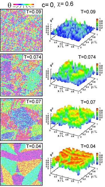
Figure 1: Orientation angles $\theta_{i}$ in the range $0<\theta_{i}<\pi$ (left) and order parameter amplitudes $q^{2}_{i}$ (right) of all the particles on a lattice in the $xy$ plane with $c=0$ and $\chi=0.6$ for $T=0.09$, $0.074$, $0.07$, and $0.04$ from above. As $T$ is lowered, orientation order develops gradually with lattice deformations.

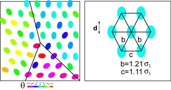
Figure 2: Left: Expanded snapshot of $\theta_{i}$ around a junction point of three variants in the bottom panel of Fig.1 at $T=0.04$. The angles among the three lines are $65$, $145$, and $150$ degrees, being approximately multiples of $\pi/6$. Right: Hexagonal lattice structure in an ordered variant composed of isosceles triangles for $\chi=0.6$ and $T=0.04$.

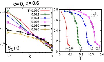
Figure 3: Left: Structure factor of the orientation fluctuations $S_{Q}(k)$ in Eq.(23) vs $k$ with $c=0$ and $\chi=0.6$ for $T=0.07,0.072,0.074,0.076,0.08$, and $0.09$, which grows algebraically for small $k<0.3$ in the BKT phase. Right: Average amplitude $\langle{q^{2}}\rangle$ in Eq.(18) vs $T$ for $\chi=0.6$, $1.2$, $1.8$, and $2.4$, which increases gradually but steeply at low $T$.

III Orientation phase transition in one-component systems

In this section, we treat pure (one-component) systems of the elliptic particles ($c=0$). We assume not large values of $\chi(\leq 2.4)$ such that the crystallization first occurs at $T=T_{m}\sim 1$ with random molecular orientations. Far below $T_{m}$, we study an orientation phase transition on a hexagonal lattice and singular mechanical behavior specific to multi-variant states. A number of authors Frenkel1 ; Rolf ; Kantor numerically examined the phase behavior of one-component hard rod systems in three dimensions in the plane of the aspect ratio and the density. If the particles are rather close to spheres, they found orientationally disordered and ordered crystal phases. Solids in the orientationally disordered phase have been called “plastic solids” Sherwood ; Frenkel1 ; Rolf ; Kantor . To understand singular mechanical properties of TiNi around its martensitic phase transition, Ding et al. Suzuki performed molecular dynamics simulation on mixtures of two species of spherical particles.

III.1 Variant formation and Berezinskii-Kosterlitz-Thouless phase

In Figs.1-3, we show our simulation results at fixed volume under the periodic boundary condition. Assuming a Nos$\acute{\rm e}$-Hoover thermostat nose , we started with a liquid at $T=2$, quenched the system to $T=0.35$ below the melting, and annealed it for $9000\tau_{0}$. We then lowered $T$ to a final low temperature. Here, even if the cooling rate was varied after the crystal formation (in the range $T<0.35$), essentially the same results followed. That is, there was no history-dependent behavior.

In Fig.1, we show the orientation angles $\theta_{i}$ of all the particles in the range $0<\theta_{i}<\pi$ (left) and the order parameter amplitudes $q^{2}_{i}$ in Eq.(17) (right) at $T=0.09,0.074$, $0.07$, and $0.04$. With lowering $T$, three equivalent variants emerge due to the underlying hexagonal lattice. Their areal fractions are all nearly equal to $1/3$. For $T=0.074$ the time scale of the patterns is of order $10^{4}$, while for $T=0.07$ and $0.04$ the patterns are frozen even on time scale of $10^{5}$. At low $T$, the junction angles, at which two or more domain boundaries intersect, are multiples of $\pi/6$. As illustrated in Fig.2, this geometrical constraint arises from the orientation-lattice coupling. It serves to pin the domain growth at a characteristic size even without impurities Onukibook . Similar pinned domain patterns have been observed on hexagonal planes Kitano and were reproduced by phase-field simulation Chen . We may define the surface tension $\gamma$ on the interfaces far from the junction regions. In our model, $\gamma\sim 0.1\epsilon/\sigma_{1}^{2}$ for $\chi=0.6$ and $\gamma\sim 0.2\epsilon/\sigma_{1}^{2}$ for $\chi=1.2$ at low $T$.

In Fig.3, the structure factor $S_{Q}(k)$ in Eq.(23) vs $k$ and the average $\langle{q^{2}}\rangle$ in Eq.(18) vs $T$ are displayed for $\chi=0.6,1.2,1.8$, and 2.4. Here, the orientation order develops continuously in a narrow temperature range,

$$T_{2}(\chi)<T<T_{1}(\chi),$$ (24)

where $T_{2}\sim 0.070$ and $T_{1}\sim 0.076$ for $\chi=0.6$. In our simulation, $T_{1}$ and $T_{2}$ increase with increasing $\chi$. They are determined as crossover temperatures. In this temperature window, a Berezinskii-Kosterlitz-Thouless (BKT) phase Jose ; Nelson is realized between the low-temperature ordered phase for $T<T_{2}$ and the high-temperature disordered phase for $T>T_{1}$, where the orientation fluctuations are strongly enhanced at long wavelengths. In our model, each elliptic particle on a lattice point behaves as a rotator in the XY spin model under a symmetry-breaking free energy $\Delta F=-\sum_{i}h_{p}\cos(p\theta_{i})$ with $p=6$, which arises from the underlying crystal structure Jose . In accord with the theory Jose ; Nelson , the structure factor $S_{Q}(k)$ in Eq.(23) grows algebraically as

$$S_{Q}(k)\sim k^{-2+\eta}\quad(k\lesssim 0.5)$$ (25)

in the temperature range (24) with $\eta$ depending on $T$ ($\eta\cong 0.05$ at $T=0.074$). As regards dynamics, the orientation fluctuations migrate in space on rather rapid time scales slightly below $T_{1}$, but are frozen for $T\lesssim T_{2}$ (see Fig.13 below). Considerably below $T_{2}$, the three variants become distinct with sharp interfaces. Previously, for two-dimensional hard rods, Bates and Frenkel Frenkel2 found a Kosterlitz-Thouless phase transition between the nematic phase and the isotropic phase for large aspect ratios and for low densities.

As illustrated in the right panel of Fig.2, the orientation order induces lattice deformations. In ordered states at low $T$, each variant is composed of isosceles triangles elongated along its orientated direction parallel to one of the crystal axes. At low $T$, their side lengths $b$ and $c$ are $(b,c)=(1.21,1.11)$ for $\chi=0.6$ and $(1.27,1,11)$ for $\chi=1.2$ under the periodic boundary condition, while we have $(b,c)=(1.28,1.12)$ at zero stress. Thus this orientation transition is also a structural or martensitic one with spontaneous lattice deformations.

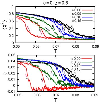
Figure 4: Order parameter amplitude $\langle{q^{2}}\rangle$ (top) and strain $\varepsilon$ (bottom) under fixed applied stress $\sigma_{a}=+0$, 0.05, 0.10, and 0.15 in units of $\varepsilon/\sigma_{1}^{2}$, where $c=0$ and $\chi=0.6$. The temperature $T$ was first decreased from 0.1 to 0.02 and it was then increased back to 0.1, where $dT/dt=\mp 4\times 10^{-6}$. Hysteretic behavior appears between the cooling and heating paths.

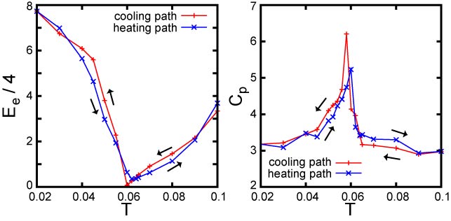
Figure 5: Young’s modulus $E_{e}$ in Eq.(28) divided by 4 (left) and the isobaric specific heat $C_{p}$ in Eq.(32) (right) for $c=0$ on the cooling and heating paths in Fig.4 in the nearly stress-free condition ($\sigma_{a}=10^{-3}$). Here $E_{e}/4$ is nearly equal to the effective shear modulus $\mu_{e}$ in Eq.(29). Softening against shear deformations and large energy fluctuations are conspicuous at the orientation transition.

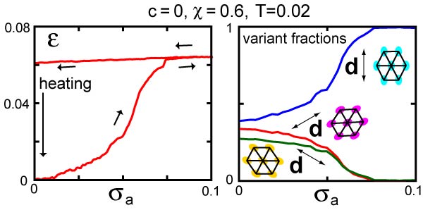
Figure 6: Shape memory effect under uniaxial deformations along the $y$ axis without impurities ($c=0$), where $T=0.02$ and $\chi=0.6$. Left: Strain $\varepsilon$ vs applied stress ${\sigma_{a}}$ in units of $\epsilon/\sigma_{1}^{2}$. For ${\sigma_{a}}>0.075$, there remains only the variant elongated along the $y$ axis. After this cycle, the residual strain vanishes upon heating to $T=0.1$. Right: Fractions of the three variants during the cycle, which are stretched along the three crystal axes.

III.2 Mechanical properties and specific heat for $c=0$

We have also performed simulation at a fixed stress Rahman , which allows an anisotropic shape change of the system at a structural phase transition. In Figs.4-7, we assumed a Nos$\acute{\rm e}$-Hoover thermostat nose and a Parrinello-Rahman barostat Rahman under the periodic boundary condition. Namely, we controlled the temperature $T$ and the stress along the $y$ axis written as

$$\sigma_{a}=\langle{\sigma_{yy}}\rangle,$$ (26)

where $\langle{\cdots}\rangle$ represents the space average. The $y$ axis is taken to be in the perpendicular direction in the figures. Hereafter, $\sigma_{a}$ will be measured in units of $\epsilon/\sigma_{1}^{2}$. When $\sigma_{a}$ was held fixed at a positive value for a long time, a single-variant state elongated along the $y$ axis was eventually realized at low $T$. This was the case even for very small positive $\sigma_{a}$ ($\sim 10^{-3}$), since it serves as a symmetry-breaking field. We also carried out many simulation runs exactly setting $\sigma_{a}=0$, where a few domains often remained in the final state depending on the initial conditions (not shown in this paper). When $\sigma_{a}$ is controlled, the system length $L_{y}$ along the $y$ axis should be calculated. The strain $\varepsilon$ is defined as

$$\varepsilon=L_{y}/L_{y0}-1,$$ (27)

where $L_{y0}$ is a reference system length to be specified below. We may define Young’s modulus by

$$E_{e}=1/(\partial\epsilon/\partial{\sigma_{a}})_{T}.$$ (28)

even in the nonlinear regime. Note that Young’s modulus is written as $E=4K\mu/(K+\mu)$ in the linear regime in terms of the bulk modulus $K$ and the shear modulus $\mu$ in two dimensions. We may introduce the effective shear modulus $\mu_{e}$ replacing $E$ by $E_{e}$ as

$$\mu_{e}=E_{e}/(4-E_{e}/K)\cong E_{e}/4,$$ (29)

where we have assumed $E_{e}\ll K$.

Substantial thermal hysteresis during cooling and heating has been observed in alloys around martensitic phase transitions marten1 ; marten2 ; marten3 . Ding et al. also found thermal hysteresis numerically Suzuki . In Fig.4, we show thermal hysteresis in our system for $c=0$. That is, fixing $\sigma_{a}$, we decreased $T$ from 0.1 to 0.02 with a very slow cooling rate given by $dT/dt=-4\times 10^{-6}$, where the variant elongated along the $y$ axis became dominant at low $T$. We then increased $T$ back to the initial high temperature with $dT/dt=4\times 10^{-6}$. The curves of $\sigma_{a}=+0$ are those with a small symmetry breaking stress ($=10^{-3}$). The reference length $L_{y0}$ in Eq.(27) is that at $T=0.09$ equal to $73.0$, $73.5$, $75.7$, and $76.2$ for $\sigma_{a}=+0$, 0.05, $0.1$, and 0.15, respectively. Hysteretic behavior can be seen in the degree of orientation $\langle{q^{2}}\rangle$ and the strain $\varepsilon$. The width of the hysteresis loop is maximum for $\sigma_{a}=+0$ and shrinks to vanish for $\sigma_{a}>0.15$. The transition at $\sigma_{a}=+0$ between the orientationally disordered and ordered states is shifted to lower temperatures by 0.01 than in the fixed-volume case in Fig.1. See Remark (4) in Sec.VII for discussions on the stability of quasi-equilibrium states in Fig.4.

When $\langle{q^{2}}\rangle$ is small, we may use the linear elasticity relations in two dimensions,

$$K[e_{1}-\alpha(T-T_{0})]+\mu(2\varepsilon-e_{1})=\sigma_{a},$$

$$K[e_{1}-\alpha(T-T_{0})]-\mu(2\varepsilon-e_{1})=0,$$ (30)

where $e_{1}$ is the dilation strain, $\alpha$ is the thermal expansion coefficient, and $T_{0}$ is a reference temperature . The small slope of the curves of $\varepsilon$ at $\sigma_{a}=+0$ in the disordered regions in Fig.4 arise from the thermal expansion. From these relations we obtain

$$e_{1} = \sigma_{a}/2K+\alpha(T-T_{0}),$$

$$\varepsilon = (K+\mu)\sigma_{a}/4K\mu+\alpha(T-T_{0})/2$$ (31)

The data in Fig.4 yield $K\cong 20$, $\alpha\cong 0.6$, and $\mu\cong 2$ with $T_{0}=0.09$ in the disordered phase.

In the left panel of Fig.5, we show Young’s modulus $E_{e}$ in Eq.(28) on the cooling and heating paths of $\sigma_{a}=+0$ in Fig.4. To calculate it, we superimposed a small stress ($=10^{-2})$ to the much smaller symmetry-breaking stress ($=10^{-3})$. Remarkably, $E_{e}$ becomes very small around $T=0.06$ for $c=0$ Cowley ; Onukibook . Similar minimum behavior of the shear modulus has been observed near the orientation and glass transitions ori ; sound ; sound1 , where the minimum depends on the mixture composition. Previously, using the correlation function expression, Murat and Kantor Kantor calculated the elastic constant to find its softening toward the orientation transition in two-dimensional ellipsoid systems. Nonlinear response behavior should appear even for very small applied strains near the transition. Additionally, in the right panel of Fig.5, we display the isobaric specific heat in the nearly stress-free condition ($\sigma_{a}=10^{-3}$) along the cooling and heating paths expressed as

$$C_{p}=\langle{({\cal H}-\langle{\cal H}\rangle)^{2}}\rangle/VT^{2},$$ (32)

where ${\cal H}=K+U$ is the total energy (see Eqs.(7) and (8)) and $\delta{\cal H}={\cal H}-\langle{{\cal H}}\rangle$ is its deviation. It is peaked at $T=0.06$ indicating enhancement of the energy fluctuations at the transition. Such specific heat anomaly has been measured near the orientation transition Yamamuro . We also calculated the constant-volume specific heat $C_{V}$ using the data in Fig.1 to find a similar peak around $T=0.073$ (not shown in this paper).

Next, we illustrate the shape memory effect taking place without dislocations. In Fig.6, we increased ${\sigma_{a}}$ from 0 to 0.1 and then decreased ${\sigma_{a}}$ back to 0 at $T=0.02$, where $d\sigma_{a}/dt=\pm 7\times 10^{-6}$ with $+$ being on the stretching path and $-$ being on the return path. In this slow cycle, the system remained in quasi-static states. In the definition of $\varepsilon$ in Eq.(27), $L_{y0}$ is the initial system length $(\cong 72)$. At $t=0$, the fractions of the three variants were nearly close to $1/3$ and one variant was elongated along the $y$ axis. In the very early stage $\varepsilon<2\times 10^{-3}$, the system deformed elastically with $\mu_{e}\cong\mu\sim 2$. However, in the next stage $2\times 10^{-3}<\varepsilon<0.075$, the fraction of the favored variant increased up to unity with $\mu_{e}\sim 0.1-0.8$. This inter-variant transformation occurred without dislocation formation. On the return path, the solid was composed of the favored variant only with large $\mu_{e}\sim 7$. As $\sigma_{a}\to 0$, there remained a remnant strain about 0.06. However, upon heating to $T=0.1$ above the transition, it disappeared and the solid again assumed a square shape. We note that plastic deformations should occur at high strains. In the present simulation, dislocations were indeed proliferated for ${\sigma_{a}}>0.4$ (or $\epsilon>0.08$) at $T=0.02$.

IV Glass formation with large repulsive impurities

In Figs.7-11, we treat mixtures of elliptic particles and large repulsive impurities. With increasing the impurity composition $c$, the orientation disorder is enhanced and the long wavelength orientation fluctuations are suppressed, resulting in “orientation-strain glass”. Here, even for our anisotropic particle systems, we predict the nonlinear mechanical behavior studied for strain glass Ren . The BKT phase disappears with increasing $c$.

IV.1 Orientation-strain glass

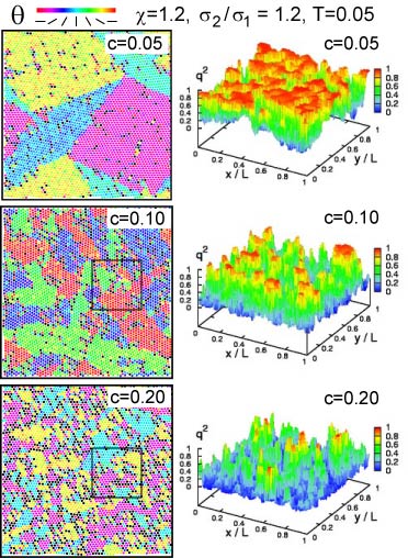
Figure 7: Frozen patterns of angles $\theta_{i}$ in the range $0<\theta_{i}<\pi$ (left) and order parameter amplitudes $q_{i}^{2}$ (right) with impurities (black points) at $c=0.05$, $0.1$ and 0.2, where $T=0.05$ and $\chi=1.2$.

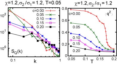
Figure 8: $S_{Q}(k)$ vs $k$ with $\chi=1.2$ and $T=0.05$ (left) and $\langle{q^{2}}\rangle$ vs $T$ with $\chi=1.2$ (right). Five curves correspond to $c=0,0.05,0.1,0.15$, and 0.2, which are gradually suppressed with increasing $c$.

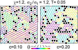
Figure 9: Expanded snapshots of $\theta_{i}$ around large impurities ($\bullet$) for $c=0.1$ and 0.2, exhibiting planar anchoring of molecular orientations and clustering.

Figures.7-9 are simulation results with a thermostat at fixed volume under the periodic boundary condition, where $T=0.05$ and $\chi=1.2$. The temperature was lowered from a high temperature as in the previous section. The size ratio is fixed at $\sigma_{2}/\sigma_{1}=1.2$. For $c\leq 0.2$, the system still forms a single hexagonal crystal with point defects at the impurity positions.

In Fig.7, we present snapshots of $\theta_{i}$ and $q_{i}^{2}$ for three compositions as in Fig.1. In the top panel at $c=0.05$, the impurities induce irregular orientation disorder, but not much affect the overall order such that large-scale domains are still distinct. In the lower panels with $c=$0.1 and 0.2, the orientation disorder increases and the domain sizes become finer. For $c=0.2$, the system approaches orientation glass but with mesoscopically ordered regions still remaining. In Fig.8, increasing $c$ gives rise to suppression of $S_{Q}(k)$ at long wavelengths ($k\lesssim 0.3$) and $\langle{q^{2}}\rangle$ in Eq.(18) at low $T$.

Figure 9 displays expanded snapshots of the elliptic particles around the impurities. We recognize that the alignments are mostly perpendicular to the surface normals, analogously to the parallel anchoring of liquid crystal molecules on the colloid surfaces Prost . Moreover, we notice an apparent tendency of string-like clustering or aggregation of the impurities. They tend to be localized along the interface regions between different variants, allowing formation of mesoscopically ordered regions of the elliptic particles even for $c=0.2$.

To examine the degree of clustering, we may group the impurities into clusters. Let the two impurities $i$ and $j$ belong to the same cluster if their distance is shorter than $1.6\sigma_{1}$. Then we obtain the numbers $N_{\rm cl}(\ell)$ of the $\ell$ clusters (those consisting of $\ell$ impurities), where $\ell=1,2,\cdots$ and $\sum_{\ell}\ell N_{\rm cl}(\ell)=N_{2}$. The probability that one impurity belongs to one of the $\ell$ clusters is $P_{\rm cl}(\ell)=\ell N_{\rm cl}(\ell)/N_{2}$. The average cluster size is defined as

$${\bar{\ell}}_{\rm cl}=\sum_{\ell}\ell P_{\rm cl}(\ell)=\sum_{\ell}\ell^{2}N_{\rm cl}(\ell)/N_{2}$$ (33)

In Fig.7, we have ${\bar{\ell}}_{\rm cl}=1.37$, 2.04, and 4.79 for $c=0.05$, 0.1, and $0.2$, respectively.

IV.2 Mechanical properties in glass

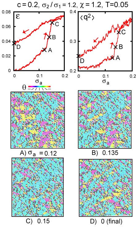
Figure 10: Shape memory effect under uniaxial deformations along the $y$ axis with impurities, where $T=0.05$, $c=0.2$, and $\chi=1.2$. Top: $\varepsilon$ vs ${\sigma_{a}}$ (left) and $\langle{q^{2}}\rangle$ vs ${\sigma_{a}}$ (right). For $0.12<\sigma_{a}<0.155$, $\varepsilon$ and $\langle{q^{2}}\rangle$ increase steeply. For ${\sigma_{a}}>0.15$, there remains only the variant elongated along the $y$ axis. After this cycle, the residual strain is 0.04, which vanishes upon heating to $T=0.1$. Bottom: Snapshots of $\theta_{i}$ for $\sigma_{a}=0.12,0.135$, and 0.15 in the transition region, where large-scale orientation fluctuations can be seen but there is no dislocation.

We also observed a shape-memory effect even in orientation glass, where small disfavored domains were gradually replaced by favored ones upon stretching. In this effect, no dislocation was formed at low $T$.

In Fig.10, at $T=0.05$, we increased $\sigma_{a}$ slowly at $d\sigma_{a}/dt=4\times 10^{-6}$ from 0 up to 0.2, where the variant elongated along the $y$ axis becomes increasingly dominant. We then decreased $\sigma_{a}$ back to 0 at $d\sigma_{a}/dt=-4\times 10^{-6}$. Between these two paths, significant differences can be seen in the degree of orientation $\langle{q^{2}}\rangle$ and the strain $\varepsilon$. The $\varepsilon$ is given by Eq.(27) with $L_{y0}$ being the initial system length at $T=0.05$ and $\sigma_{a}=+0$. On the stretching path, there appear four stress ranges: $\mu_{e}\sim 3$ for $0<\sigma_{a}<0.05$, $\mu_{e}\sim 0.8$ for $0,05<\sigma_{a}<0.12$, $\mu_{e}\sim 0.2$ for $0.12<\sigma_{a}<0.15$. Remarkably, the response is elastic in the first range and is very large with $\varepsilon$ increasing steeply from $0.028$ to $0.064$ in the third range. For $\sigma_{a}>0.15$ and on the return path, $\mu_{e}$ is of order unity and we can see considerable variations in $\varepsilon$ and $\langle{q^{2}}\rangle$, where the fractions of the disfavored variants significantly change around the impurities. In contrast, in the one-component case in Fig.6, we have found no such changes once a single-variant state is realized.

In the bottom panels of Fig.10, we display snapshots of $\theta_{i}$ at four points A, B, C, and D where $\sigma_{a}=0.12,0.135$, 1.5, and 0, respectively. See the bottom left panel of Fig.7 for the snapshot at the initial time in the same run. Between A and B, the orientation and the strain increase abruptly. In this transition region, we notice emergence of large-scale orientation fluctuations taking stripe shapes and making angles of $\pm\pi/4$ with respect to the $x$ axis. In stress and thermal cycles in glass, the impurities pin the orientation fluctuations in quasi-stationary states under very slow time variations of $\sigma_{a}$ and $T$, yielding the history-dependence of the physical quantities.

IV.3 Positional disorder for $\sigma_{2}/\sigma_{1}=1.4$

So far, the crystal structure has been little affected by the orientation fluctuations at $\sigma_{2}/\sigma_{1}=1.2$ for $c=0.1$ and 0.2. However, if we adopt a larger size ratio and/or a larger composition, the positional (structural) disorder is increasingly enhanced, resulting in usual positional polycrystal or glass. In our case, the orientation disorder is more enhanced than the positional disorder. This is in sharp contrast to liquid crystal systems where the nematic order precedes the crystallization.

In Fig.11, we set $\sigma_{2}/\sigma_{1}=1.4$ and $\chi=1.2$ to obtain polycrystal for $c=0.1$ and 0.2. In the left, the orientation angles $\theta_{j}$ are displayed, where there still remains noticeable mesoscopic orientation order. In the left, sixfold bond-orientation (crystal) angles $\alpha_{j}$ are displayed, where we introduce $\alpha_{j}$ for each elliptic particle $j$ in the range $0\leq\alpha_{j}<\pi/3$ by Nelson ; Hama

$$\sum_{k\in\textrm{\scriptsize{bonded}}}\exp[6i\theta_{jk}]=Z_{j}\exp[{6i\alpha_{j}}],$$ (34)

Here, $\theta_{jk}$ is the angle of the relative position vector ${\mbox{\boldmath$r$}}_{jk}={\mbox{\boldmath$r$}}_{k}-{\mbox{\boldmath$r$}}_{j}$ with respect to the $x$ axis, the particle $k$ is within the range $|{\mbox{\boldmath$r$}}_{jk}|<1.7\sigma_{1}$, and $Z_{j}$ and $6\alpha_{j}$ are the absolute value and the phase angle of the left hand side, respectively. For $c=0.1$, one large grain is embedded in a crystal containing many point defects, where angle differences are of order $10-15$ degrees. On the other hand, for $c=0.2$, many grains appear with much larger angle differences.

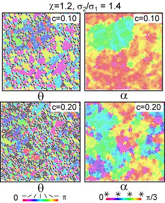
Figure 11: Orientation angle $\theta_{i}$ in the range $0<\theta_{i}<\pi$ (left) and sixfold bond orientation angle $\alpha_{i}$ in Eq.(34) in the range $0<\theta_{i}<\pi/3$ (right) in polycrystal states for $c=0.1$ (top) and 0.2 (bottom), where $\chi=1.2$ and $T=0.05$. The size ratio is increased to $\sigma_{2}/\sigma_{1}=1.4$.

V Rotational dynamics

V.1 Angle relaxation functions

We now discuss the rotation dynamics of the elliptic particlesChong ; new . In two dimensions, we consider the time-dependent angle-distribution function defined by

$$G(t,\varphi)=\frac{1}{N_{1}}\sum_{1\leq j\leq N_{1}}\langle{\delta(\theta_{j}(t+t_{0})-\theta_{j}(t_{0})-\varphi)}\rangle,$$ (35)

where the average $\langle{\cdots}\rangle$ is taken over the initial time $t_{0}$ and over several runs. Here, $G(t,\varphi)$ tends to $\delta(\varphi)$ as $t\to 0$ and is broadened for $t>0$. In particular, we treat the first two moments $G_{1}(t)$ and $G_{2}(t)$ written as

$$G_{1}(t) = \int_{0}^{2\pi}{d\varphi}G(t,\varphi)\cos(\varphi),$$ (36)

$$G_{2}(t) = \int_{0}^{2\pi}d\varphi G(t,\varphi)\cos(2\varphi).$$ (37)

Since these two functions are unity as $t\to 0$, we introduce two relaxation times, $\tau_{1}$ and $\tau_{2}$, by

$$G_{1}(\tau_{1})=e^{-1},\quad G_{2}(\tau_{2})=e^{-1}.$$ (38)

These times grow as $T$ is lowered. We plot $G_{1}(t)$ and $G_{2}(t)$ vs $t$ in Fig.12 and $\tau_{1}$ vs $T$ in Fig.13.

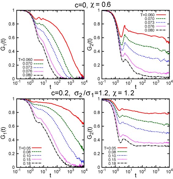
Figure 12: Orientation relaxation functions $G_{1}(t)$ (left) and $G_{2}(t)$ (right) in Eqs.(36) and (37) for $c=0$ and $\chi=0.6$ (top) and for $c=0.2$, $\sigma_{2}/\sigma_{1}=1.2$, and $\chi=1.2$ (bottom). Relaxations are slowed down as $T$ is lowered. The $G_{1}(t)$ decays due to turnover motions, while $G_{2}(t)$ due to configuration changes. For $c>0$, $G_{2}(t)$ tends to a finite constant as $t\to\infty$.

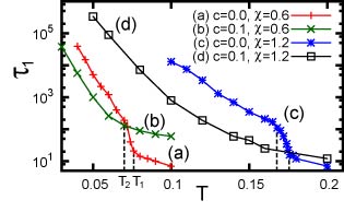
Figure 13: Orientation relaxation time $\tau_{1}$ from $G_{1}(t)$ for (a) $c=0$ and $\chi=0.6$, (b) $c=0.1$ and $\chi=0.6$, (c) $c=0$ and $\chi=1.2$, and (d) $c=0.1$ and $\chi=1.2$. It is the time scale of successive turnover motions. For (a) and (c), $\tau_{1}$ grows steeply in the BKT phase ($T_{2}<T<T_{1}$). For strain glass (b) and (d), the BKT phase is nonexistent and $\tau_{1}$ grows as $T$ is lowered.

V.2 Turnover motions and configuration changes

As a marked feature, the elliptic particles sometimes undergo the turnover motion $\theta_{j}\to\theta_{j}\pm\pi$ or ${\mbox{\boldmath$n$}}_{j}\to-{\mbox{\boldmath$n$}}_{j}$ taking place in a microscopic time $(\sim 1$)new . In terms of the orientation vector ${\mbox{\boldmath$n$}}_{j}$, we also have

$$G_{1}(t)=\sum_{1\leq j\leq N_{1}}\langle{{\mbox{\boldmath$n$}}_{j}(t+t_{0})\cdot{\mbox{\boldmath$n$}}_{j}(t_{0})}\rangle/N_{1},$$ (39)

so that the times between successive turnovers of an elliptic particle are of order $\tau_{1}$ in Eq.(38). On the average over all the elliptic particles, the turnover motions give rise to a peak in $G(t,\varphi)$ at $\varphi=\pi$.

In our simulation, it is nearly of the Gaussian form for $t\ll\tau_{1}$ in the range $|\varphi-\pi|\lesssim 1$ as

$$G(t,\varphi)\cong\frac{A(t)}{\sqrt{2\pi}\sigma}\exp\bigg{[}-\frac{(\varphi-\pi)^{2}}{2\sigma^{2}}\bigg{]},$$ (40)

where the variance $\sigma$ is a constant about $0.45$ in the present case. The integral of this Gaussian peak is equal to the coefficient $A(t)$, so $A(t)$ has the meaning of the turnover probability per elliptic particle in the time interval $[0,t]$. In terms of $\tau_{1}$, we find the linear growth,

$$A(t)\cong C_{1}t/\tau_{1},$$ (41)

in the early time range $t\ll\tau_{1}$. In our system $C_{1}\cong 0.5$. On the other hand, $G_{2}(t)$ is unchanged by the instantaneous turnover motions, so it relaxes due to the orientational configuration changes involving the surrounding particles. We found the inequality $\tau_{2}>\tau_{1}$ at any $T$ and $c$ in our simulation.

In Fig.12, both $G_{1}(t)$ and $G_{2}(t)$ relax considerably in the early time region $t\lesssim 2$ due to the thermal rapid motions of the orientations without configuration changes. For $t\gtrsim 2$ the fitting $G_{1}(t)\sim\exp[-(t/\tau_{1})^{\beta}]$ fairly holds, where $\beta$ decreases from unity to about 0.5 as $T$ is lowered. Furthermore, for $c>0$, $G_{2}(t)$ tends to a nonvanishing positive constant $f_{2}$ at large $t$ Chong . In our case, this plateau appears because the anchoring of the elliptic particles around the impurities becomes nearly permanent at low $T$. Thus we found that the plateau height $f_{2}$ increases with lowering $T$ and with increasing $c$.

In Fig.13, the two curves for $c=0$ indicate that $\tau_{1}$ is short ($\lesssim 10)$ for $T\gtrsim T_{1}$, increases steeply in the BKT region $T_{2}\lesssim T\lesssim T_{1}$, and grows further in the ordered region $T\lesssim T_{2}$ in the thermal activation form,

$$\tau_{1}\sim\exp(T_{0}/T)\quad(T\lesssim T_{2}).$$ (42)

We have $T_{0}\sim 0.40$ at $\chi=0.6$ on curve (a) and $T_{0}\sim 1.2$ at $\chi=1.2$ on curve (c). In addition, $\tau_{1}\sim\tau_{2}$ for $T\gtrsim T_{1}$ but $\tau_{2}/\tau_{1}\gg 1$ for $T\lesssim T_{2}$. In fact, for $\chi=0.6$, $\tau_{2}/\tau_{1}$ is about $10^{2}$ at $T=0.07$ and is about $10^{3}$ at $T=0.06$.

For $c>0$, the turnover motions still occur with $\tau_{1}<\tau_{2}$. However, in Fig.13, the relaxation behavior for $c>0$ is very different from that for $c=0$. In the disordered phase with $T\gtrsim T_{1}$, $\tau_{1}$ for $c>0$ is longer than $\tau_{1}$ for $c=0$ due to the impurity pinning. For $T\lesssim T_{2}$, on the contrary, $\tau_{1}$ for $c>0$ is shorter than $\tau_{1}$ for $c=0$. That is, the turnover motions are more frequent in orientation glass with $c>0$ than in the orientationally ordered phase with $c=0$, as ought to be the case. Above $T_{2}$, the impurity anchoring gradually becomes transient.

It is worth noting that Chong et al Chong studied the orientation dynamics of a glass-forming binary mixture of dumbbells using the angle relaxation functions $C_{\ell}(t)=\sum_{j}\langle{P_{\ell}({\mbox{\boldmath$n$}}_{j}(t_{0}+t)\cdot{\mbox{\boldmath$n$}}_{j}(t_{0})}\rangle/N$ in three dimensional molecular dynamics simulation, where $P_{\ell}$ is the Legendre polynomial of order $\ell$ and ${\mbox{\boldmath$n$}}_{j}$ is the orientation vector of particle $j$. The relaxations of $C_{1}(t)$ and $C_{2}(t)$ for small dumbbell anisotropy in their paper closely resemble those of $G_{1}(t)$ and $G_{2}(t)$ for $c=0.2$ in Fig.12.

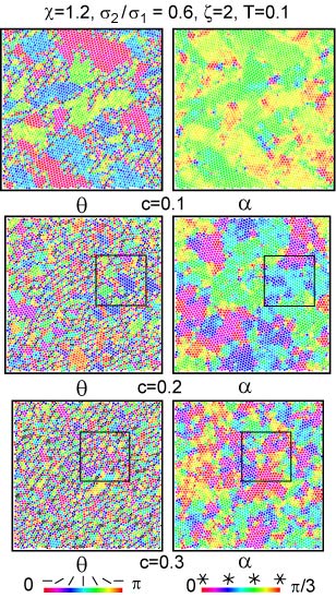
Figure 14: Snapshots of orientation angles $\theta_{i}$ (left) and sixfold crystal angles $\alpha_{i}$ with addition of small attractive impurities with $c=0.1$ (top), 0.2 (middle), and 0.3 (bottom), where $T=0.1$, $\chi=1.2,$ $\sigma_{2}/\sigma_{1}=0.6$, and $\zeta=2$. The orientation disorder is stronger than the positional disorder. The cooling rate from $T=1$ to 0.1 is $dT/dt=-1.8\times 10^{-5}$.

VI Glass formation with small attractive impurities

In this section, we further treat another intriguing case of small attractive impurities with $\sigma_{2}/\sigma_{1}=0.6$ in Eq.(3) and with $\zeta=2$ in Eq.(6). Such small impurities tend to be expelled from the ordered domains of the host particles. We shall see that they form clusters.

VI.1 Orientational disorder and positional disorder

Though not shown in this paper, we performed simulation runs for small repulsive impurities with $\sigma_{2}/\sigma_{1}=0.6$ and $\zeta=0$, where most of the impurity aggregates are stringlike and the anchoring of the elliptic particles is planar. However, if the anisotropy strength of attraction $\zeta$ is increased at fixed $\chi$, the aggregates becomes increasingly compact. For $\zeta\gtrsim 1$, the aggregates can “solvate” several elliptic particles in the homeotropic alignmentProst . With further increasing $\zeta$, even a single impurity creates a solvation shell composed of several elliptic particles like a small metallic ion in water.

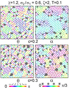
Figure 15: Expanded snapshots of elliptic particles and small attractive impurities (black points) in the boxes in Fig.14, where homeotropic anchoring and impurity clustering are marked. Colors of the elliptic particles represent the orientation angles $\theta_{j}$ (left) and the sixfold crystal angles $\alpha_{j}$ (right) from the same data. The domains (left) are finer than the grains (right). The cooling rate from $T=1$ to 0.1 is $dT/dt=-1.8\times 10^{-5}$.

In Fig.14, we show snapshots of $\theta_{j}$ and $\alpha_{j}$ of all the particles, where $T=0.1$, $\chi=1.2,$ $\sigma_{2}/\sigma_{1}=0.6$, and $\zeta=2$. Here, we set $dT/dt=-1.8\times 10^{-5}$. For $c=0.1$, the system is still in a single crystal state, but the orientational domain structure induces large-scale elastic deformations, leading to close resemblance of the patterns of $\theta_{j}$ and $\alpha_{j}$. For $c=0.2$, the orientational domains are much finer and a polycrystal state is realized with larger grains ($\gtrsim 10$). For $c=0.3$, the orientation order is much more suppressed and a positional glass state is realized with mesoscopic heterogeneities still remaining.

In Fig.15, we display expanded snapshots of $\theta_{j}$ (left) and $\alpha_{j}$ in Eq.(34) (right) in the box regions in Fig.14. The alignments of the elliptic particles around the impurities are mostly parallel to the surface normals. This is analogous to the homeotropic anchoring of liquid crystal molecules on the colloid surfaces Prost . We notice a tendency of clustering or aggregation of the impurities. Comparing the left and right panels, we recognize that the interfaces are finer than the grain boundaries. That is, the interfaces can be seen both on the grain boundaries and within the grains. The impurities tend to be localized on the interface regions between different variants.

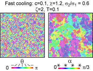
Figure 16: Snapshots of orientation angles $\theta_{i}$ (left) and sixfold crystal angles $\alpha_{i}$ (right) with addition of small attractive impurities with $c=0.1$. The parameter values are common to those in the top panel of Fig.14, but the cooling rate from $T=1$ to 0.1 is $dT/dt=-9\times 10^{-3}$. Here, the degree of clustering is weaker, resulting in a polycrystal state.

VI.2 Cooling-rate dependent clustering of impurities

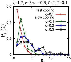
Figure 17: Probability $P_{\rm cl}(\ell)=\ell N_{\rm cl}(\ell)/N_{2}$ of an impurity belonging to $\ell$ clusters, where $N_{\rm cl}(\ell)$ is the cluster number composed of $\ell$ impurities. Here small attractive impurities are considered for slow cooling in Fig.14 and fast cooling in Fig.16. Distribution is broader for slower cooling.

The degree of impurity clustering should be decreased with increasing the cooling rate $dT/dt$ for long diffusion times of impurities. In Fig.16, $dT/dt$ is $-9\times 10^{-3}$ and is 500 times faster than in Fig.14, where the other parameters are common. We give snapshots of $\theta_{j}$ and $\alpha_{j}$ at $c=0.1$, where the clustering can be more evidently seen than for $c=0.2$ and 0.3. While a single crystal has been realized in the top panel of Fig.14, a polycrystal state is realized with large angle differences in Fig.16.

Let the two small impurities $i$ and $j$ belong to the same cluster if their distance is shorter than $1.2\sigma_{1}$. Then we obtain the number $N_{\rm cl}(\ell)$ of clusters composed of $\ell$ impurities. In Fig.17, we show the cluster size distribution $P_{\rm cl}(\ell)=\ell N_{\rm cl}(\ell)/N_{2}$ ($\ell=1,2,\cdots$) for the examples in Figs.14 and 16. The average cluster size $\bar{\ell}_{\rm cl}$ in Eq.(33) increases with $c$ as $2.45$ for $c=0.1$, 3.43 for $c=0.2$, and 4.61 for $c=0.3$ under the slow cooling in Fig.14, while $\bar{\ell}_{\rm cl}=1.62$ for $c=0.1$ under the fast cooling in Fig.16.

It is known water that water becomes glass at low $T$ with addition of a considerable amount of LiCl, where small hydrophilic Li⁺ and Cl^- ions solvate several water molecules via the strong ion-dipole interaction. The resultant orientation anchoring of water molecules should even prevent formation of the crystal order at high salt concentrations, resulting in the observed positional glass. It is natural that the cooling rate influences the degrees of ion clustering and vitrification.

VII Summary and remarks

We have presented an angle-dependent Lennard-Jones potential for elliptic particles and impurities, which depends on the orientation angles of the interacting particles. Using this potential, we have performed simulation of 4096 particles on very long time scales ($\sim 10^{5}\tau_{0}$) in two dimensions. Our main results are as follows.
(i) In Sec.II, we have presented our model potential, where the anisotropy strengths are characterized by $\chi$ for the repulsive part in Eq.(5) and $\zeta$ for the attractive part in Eq.(6). The aspect ratio of the elliptic particles is given by $a_{\ell}/a_{s}=(1+2\chi)^{1/6}$. In this paper, $\chi$ is of order unity, so we have assumed weak particle anisotropy to find crystallization at a high temperature above the orientation transition.
(ii)In Sec.III, we have presented simulation results for one-component systems of elliptic particles by changing the temperature $T$ to produce Figs.1-6. The domain patterns in Fig.1 at low $T$ are those observed on hexagonal planes. In our case, the Berezinskii-Kosterlitz-Thouless phaseJose ; Nelson is realized in a temperature window, where the orientation fluctuations are much enhanced at long wavelengths as indicated by the structure factor $S_{Q}(k)$ in Fig.3. We have shown thermal hysteresis in Fig.4, singular behaviors of the shear modulus and the specific heat in Fig.5, and a shape-memory effect in Fig.6.
(iii) In Sec.IV, we have examined orientation-strain glass of elliptic particles and large repulsive impurities with the size ratio $\sigma_{2}/\sigma_{1}=1.2$ in Figs.7-10. The orientations of the elliptic particles are pinned at the impurity surfaces in the planar alignment in Fig.9. The shape-memory effect in strain glass is marked in Fig.10. Positional disorder also emerges for $\sigma_{2}/\sigma_{1}=1.4$ in Fig.11.
(iv) In Sec.V, we have studied the rotational dynamics of the elliptic particles. In Fig.12, $G_{1}(t)$ decays due to the turnover motions of the elliptic particles, while $G_{2}(t)$ decays due to the configuration changes. In Fig.13, the turnover relaxation time $\tau_{1}$ grows at low $T$ and behaves differently with and without impurities.
(v) In Sec.VI, we have examined the effect of small attractive impurities on the orientation disorder and the positional disorder in Fig.14. The impurity effect is stronger on the former than on the the latter. The elliptic particles are homeotropically anchored at the impurity surfaces in Fig.15. The clustering of impurities is suppressed for rapid cooling as in Figs.16 and 17.

We further make critical remarks as follows:
(1) In our simulation, we used a Nos$\acute{\rm e}$-Hoover thermostat (NHT) nose in all the figures and a NHT and a Parrinello-Rahman barostat Rahman in Figs.4-6, and 10. In future work, we should examine the coupled dynamics of the translational and orientational degrees of freedom Bell without thermostats and barostats in the system interior.
(2) There has been no systematic measurement of the mechanical properties of orientationally ordered, multi-variant crystal and orientation glass. Such experimental results could be compared with those from shape-memory alloys marten1 ; marten2 ; marten3 ; RenReview ; Ren . Weak elasticity was observed in orientationally disordered solids above the transition (called “plastic solids”) in creep experiments Sherwood . Also, as far as the authors are aware, there has been no experimental information of the impurity clustering in any physical systems exhibiting mesoscopic heterogeneities.
(3) In this paper, the particle anisotropy is not large, which favors formation of crystal order. For large anisotropy, liquid crystal phases should appear Frenkel1 ; Rolf , where the impurity effect is of great interest. As suggested by the experiment Yamamoto-Tanaka , addition of a considerable amount of impurities leads to the orientation order only on mesoscopic scales in liquid crystal phases. In such states, we expect large response to applied electric field.
(4) In Figs.1 and 4, our system undergoes a structural phase transition gradually in a narrow temperature window even for the one-component case. In our model, a gradual phase transition still occurs in the stress-free condition without impurities. However, we also stopped the cooling and waited for a long time ($\gg 10^{4}$) at $T=0.06$ on the stress-free cooling path in Fig.4; then, we observed a transition to the ordered single-variant phase (not shown in this paper). Thus, in future work, we need to calculate the Gibbs or Helmholtz free energy to decide whether the system is in equilibrium or in a metastable state.
(5) As well as the orientation fluctuations, the displacement fluctuations are also enhanced around the orientation transition, as indicated by Fig.5 and by the previous experiments ori ; sound ; sound1 . In addition, according to Cowley’s classification of elastic instabilities Cowley , our phase transitions belong to type-I instabilities where acoustic modes become soft in particular wave vector directions.
(6) The disordering effect induced by impurities prevents a sharp transition sound . Thus there is no sharp phase boundary between the high-temperature orientationally disordered phase and the low-temperature orientation-strain glass phase. These two phases change over gradually with varying $T$ as in the cases of positional glass transitions.
(7) Ding et al. Suzuki numerically studied the superelasticity, which arises from a stress-induced martensitic phase transition RenReview ; Ren . We also realized this phenomenon for anisotropic particles, which will be reported elsewhere.
(8) We will also report three-dimensional simulation on mixtures of spheroidal particles and spherical ones without and with the dipolar interaction. We shall see finely divided domains produced by impurities and large responses to applied strain and electric field.

- (1) U. T. Höchli, K. Knorr, and A. Loidl, Adv. Phys. 39, 405 (1990).
- (2) O. Yamamuro, H. Yamasaki, Y. Madokoro, I. Tsukushi, and T. Matsuo, J. Phys.: Condens. Matter 15, 5439 (2003).
- (3) R. M. Lynden-Bell and K. H. Michel, Rev, Mod. Phys. 66, 721 (1994).
- (4) K. Knorr, U. G. Volkmann, and A. Loidl, Phys. Rev. Lett. 57, 2544 (1986).
- (5) J. O. Fossum and C. W. Garland, J. Chem. Phys. 89, 7441 (1988).
- (6) The Plastically crystalline state: orientationally disordered crystals, edited by John N. Sherwood (John Wiley Sons, Chichester, 1979).
- (7) H. Warlimont and L. Delaey, Progr. Mater. Sci. 18, 1 (1974).
- (8) L. Kaufman and M. Cohen, Prog. Metal Phys. 7, 165 (1958); H. C. Tong and C. M. Wayman, Acta Metall. 22, 887 (1974); I. Cornelis and C. M. Wayman, Scripta Metall. 10, 359 (1976).
- (9) D. P. Dautovich and G. R. Purdy, Can. Met. Quart. 4, 129 (1965); G. D. Sandrock, A. J. Perkins, and R. F. Hehemann, Met. Trans. 2, 2769 (1971).
- (10) K. Otsuka and X. Ren, Prog. Mater. Sci. 50, 511 (2005).
- (11) S. Sarkar, X. Ren, and K. Otsuka, Phys. Rev. Lett. 95, 205702 (2005); Y. Wang, X. Ren, and K. Otsuka, Phys. Rev. Lett. 97, 225703 (2006).
- (12) B. E. Vugmeister and M. D. Glinchuk, Rev. Mod. Phys. 62, 993 (1990).
- (13) R. A. Cowley, S. N. Gvasaliya, S. G. Lushnikov, B. Roessli, and G. M. Rotaru, Adv. Phys. 60, 229 (2011).
- (14) K. Hirota, S. Wakimoto, and D. E. Cox, J. Phys. Soc. Jpn. 75, 111006 (2006).
- (15) A. Karim, J. F. Douglas, G. Nisato, D.-W. Liu, and E. J. Amis, Macromolecules 32, 5917 (1999).
- (16) J. Yamamoto and H. Tanaka, Nature 409, 321 (2001).
- (17) E. S. Matsuo, M. Orkisz, S.-T. Sun, Y. Li and T. Tanaka, Macromolecules, 27, 6791 (1994); F. Ikkai and M. Shibayama, Phys. Rev. Lett. 82, 4946 (1999).
- (18) E. Mendes, R. Oeser, C. Hayes, F. Boué and J. Bastide, Macromolecules 29, 5574 (1996).
- (19) L. Golubović and T. C. Lubensky, Phys. Rev. Lett. 63, 1082 (1989); A. Onuki, J. Phys. II 2, 45 (1992); S. Panyukov and Y. Rabin, Phys. Rep. 269, 1 (1996).
- (20) A. Onuki, Phase Transition Dynamics (Cambridge University Press, Cambridge, 2002).
- (21) P. G. de Gennes, C. R. Acad. Sci., Ser. B 281, 101 (1975).
- (22) M. Warner and E. M. Terentjev, Liquid crystal elastomers (Cambridge University Press, Cambridge, 2003).
- (23) J. Kpfer and H. Finkelmann, Macromol. Chem. Phys. 195, 1353 (1994); Y. Yusuf, J.-H. Huh, P. E. Cladis, H. R. Brand, H. Finkelmann, and S. Kai, Phys. Rev. E 71, 061702 (2005); K. Urayama, E. Kohmon, M. Kojima, and T. Takigawa, Macromolecules 42, 4084 (2009).
- (24) N. Uchida, Phys. Rev. E 62, 5119 (2000).
- (25) S. Sacanna and D. J. Pine, Current Opinion in Colloid Interface Science 16, 96 (2011); A. F. Demirörs, P. M. Johnson, C. M. van Kats, A. van Blaaderen, and A. Imhof, Langmuir 26, 14466 (2010).
- (26) Z. Zheng, F. Wang, and Y. Han, Phys. Rev. Lett. 107, 065702 (2011).
- (27) K. H. Michel, Phys. Rev. Lett. 57, 2188 (1986).
- (28) V. Westphal, W. Kleemann, and M. D. Glinchuk, Phys. Rev. Lett. 68, 847 (1992).
- (29) R. Vasseur and T. Lookman, Phys. Rev. B 81, 094107 (2010); N. Shankaraiah, K. P. N. Murthy, T. Lookman, and S. R. Shenoy, Phys. Rev. B 84, 064119 (2011).
- (30) S. Kartha, T. Castán, J. A. Krumhansl, and J. P. Sethna, Phys. Rev. Lett. 67, 3630 (1991); S. Kartha, J. A. Krumhansl, J. P. Sethna, and L. K. Wickham, Phys. Rev. B 52, 803 (1995).
- (31) P. Lloveras, T. Castán, M. Porta, A. Planes, and A. Saxena, Phys. Rev. B 80, 054107 (2009).
- (32) X. Ren, Y. Wang, K. Otsuka, P. Lloveras, T. Castán, M. Porta, A. Planes, and A. Saxena, MRS Bull. 34, 838 (2009).
- (33) T. Hamanaka and A. Onuki, Phys. Rev. E 74, 011506 (2006); H. Shiba and A. Onuki, Phys. Rev. E 81, 051501 (2010); T. Kawasaki and A. Onuki, J. Chem. Phys. 135, 174109 (2011).
- (34) C. A. Angell, Chem. Rev. 102, 2627 (2002); B. Prével, J. F. Jal, J. Dupuy-Philon, and A. K. Soper, J. Chem. Phys. 103, 1886 (1995); M. Kobayashi and H. Tanaka, Phys. Rev. Lett. 106, 125703 (2011).
- (35) P. G. de Gennes and J. Prost, The Physics of Liquid Crystals (Clarendon, Oxford, 1993).
- (36) S. Nosé, Mol. Phys. 52, 255 (1984).
- (37) J. G. Gay and B. J. Berne, J. Chem. Phys. 74, 3316 (1981); J. T. Brown, M. P. Allen, E. M. del Rio, and E. Miguel, Phys. Rev. E 57, 6685 (1998).
- (38) H. Shintani and H. Tanaka, Nat. Phys. 2, 200 (2006).
- (39) J. M. Drouffe, A. C. Maggs and S. Leibler, Science 254, 1353 (1991).
- (40) H. Noguchi, J. Chem. Phys. 134, 055101 (2011).
- (41) D. Frenkel and B. M. Mulder, Mol. Phys. 55, 1171 (1985); P. Bolhuis and D. Frenkel, J. Chem. Phys. 106, 666 (1997).
- (42) C. Vega and P. A. Monson, J. Chem. Phys. 107, 2696 (1997); C. De Michele, R. Schilling, and F. Sciortino, Phys. Rev. Lett. 98, 265702 (2007); M. Marechal and M. Dijkstra, Phys. Rev. E 77, 061405 (2008); M. Radu, P. Pfleiderer, and T. Schilling, J. Chem. Phys. 131, 164513 (2009).
- (43) M. Murat and Y. Kantor, Phys. Rev. E 74, 031124 (2006).
- (44) X. Ding, T. Suzuki, X. Ren, J. Sun, and K. Otsuka, Phys. Rev. B 74, 104111 (2006).
- (45) R. Sinclair and J. Dutkiewicz, Acta Metell. 25, 235 (1977); Y. Kitano, K. Kifune, and Y. Komura, J. Phys. (Paris) 49, C5-201 (1988); C. Manolikas and S. Amelinckx, Phys. Stat. Sol. (a) 60, 607 (1980); ibid. 61, 179 (1980).
- (46) Y. H. Wen, Y. Wang, and L. Q. Chen, Phil. Mag. A. 80, 1967 (2000); Y. H. Wen, Y. Wang, L. A. Bendersky, and L. Q. Chen, Acta Mater. 48, 4125 (2000).
- (47) J. V. José, L. P. Kadanoff, S. Kirkpatrick, and D. R. Nelson, Phys. Rev. B 16, 1217 (1977).
- (48) D. R. Nelson and B. I. Halperin, Phys. Rev. B 19, 2457 (1979).
- (49) M. A. Bates and D. Frenkel, J. Chem. Phys. 112, 10034 (2000).
- (50) M. Parrinello and A. Rahman, J. Appl. Phys. 52, 7182 (1981).
- (51) R. A. Cowley, Phys. Rev. B 13, 4877 (1976).
- (52) S.-H. Chong, A. J. Moreno, F. Sciortino, and W. Kob, Phys. Rev. Lett. 94, 215701 (2005).
- (53) N. B. Caballero, M. Zuriaga, M. Carignano, and P. Serra, J. Chem. Phys. 136, 094515 (2012).