Accurate emulators for large-scale computer experiments

Abstract

Large-scale computer experiments are becoming increasingly important in science. A multi-step procedure is introduced to statisticians for modeling such experiments, which builds an accurate interpolator in multiple steps. In practice, the procedure shows substantial improvements in overall accuracy, but its theoretical properties are not well established. We introduce the terms nominal and numeric error and decompose the overall error of an interpolator into nominal and numeric portions. Bounds on the numeric and nominal error are developed to show theoretically that substantial gains in overall accuracy can be attained with the multi-step approach.

and

t1Supported by Singapore National Medical Research Council Grant IRG10nov006 and an NUS Initiative to Improve Health in Asia, Global Asia Institute grant.

t2Supported by NSF Grant CMMI 0969616, NSF Career Award DMS-10-55214 and an IBM Faculty Award.

1 Introduction

Computer experiments use complex mathematical models implemented in large computer codes to study real systems. In many situations, a physical experiment is not feasible because it is unethical, impossible, inconvenient or too expensive. A mathematical model of the system can often be developed and input/output pairs can be produced with the help of computers. Typically, the input/output pairs are expensive in the sense that they require a great deal of time and computing to obtain and they are nearly deterministic in the sense that a particular input will produce almost the same output if given to the computer experiment on another occasion. Computer experiments are widely used in systems biology, engineering design, computational biochemistry, climatology and epidemiology and their pervasiveness in science, engineering and medicine is only growing. When using a computer experiment to study a real system, a thorough exploration of the surface is typically wanted. However, obtaining input/output pairs is often too expensive for a complete exploration. A solution is to evaluate the computer experiment at several well-distributed data sites given by a space-filling design mcb79 , owen92 , tang93 , flwz00 , niederreiter , owen1995 , jh08 . Then build an interpolator which can be used as a stand-in, or emulator, for the actual computer experiment. The thorough exploration of the complex surface can then be carried out on the interpolator. Excellent overviews on data collection and modeling for computer experiments can be found in SSW1989 , SWMW1989 , CMMY1991 , koehowen96 , santner , fang .

To emulate the output from a computer experiment, Gaussian process (GP) models or reproducing kernel Hilbert space (RKHS) interpolators are often used. These interpolators have a simple form and control the smoothness of the emulator. In particular, let $f$ denote the output of a run of the computer experiment, so that the functional link between input $x$ and output $y$ is $y=f(x)$. Take $\Phi\dvtx\Omega\times\Omega\to\mathbb{R}$ to be symmetric in its two arguments and positive definite. The kernel $\Phi$ is positive definite on a domain of interest $\Omega$ if

$$\sum_{i=1}^{n}\sum_{j=1}^{n}\alpha_{i}\alpha_{j}\Phi(x_{i},x_{j})>0$$

for every nonzero $\alpha\in\mathbb{R}^{n}$ and distinct $\{x_{1},\ldots,x_{n}\}\subseteq\Omega$. Then, given distinct input sites $X=\{x_{1},\ldots,x_{n}\}$, the GP or RKHS interpolator has the simple form

$$\mathcal{P}(x)=\sum_{i=1}^{n}\alpha_{i}\Phi(x,x_{i}),$$

where $\alpha$ has $A_{X}\alpha=f|_{X}$, $A_{X}=\{\Phi(x_{i},x_{j})\}$ and $f|_{X}=(f(x_{1})\cdots f(x_{n}))^{\prime}$. Associated with each symmetric, positive definite kernel is exactly one Hilbert space of functions whose norm, in the case that the kernel is smooth, measures both size and smoothness. For a particular kernel $\Phi$, this associated function space will be called its native space and will be denoted $\mathcal{N}_{\Phi}(\Omega)$. Native spaces will be discussed further in Section 5. The smoothness of the emulator is controlled in the sense that the RKHS interpolator has the smallest possible native space norm of any function interpolating $f|_{X}$ fasshauer , wahba , wendland2005 . It is worth noting that the GP models often used in practice to build emulators for computer experiments are essentially a special case of RKHS emulators. In the GP context, the kernel $\Phi$ is a, possibly scaled, correlation function. In the case that a nonzero mean function $\hat{\mu}$ is estimated in the GP model, the interpolator is actually the sum of this estimated mean function and an RKHS interpolator of the residual $(f-\hat{\mu})|_{X}$. Here, we consider translation invariant, or stationary, kernels so that $\Phi$ is a function of only the difference between its arguments. Hereafter, $\Phi(x,y)$ will be written as $\Phi(x-y)$. Note that the connection between Gaussian processes and RKHS was also discussed in wahba .

Many of the systems which scientists, engineers and medical researchers use computer experiments to study exhibit extremely complex behavior in portions of the input space. To discover and understand these regions requires a large-scale computer experiment with many input sites which are potentially very near one another. Unfortunately, most methods for building emulators, including RKHS and GP interpolators, suffer from increasingly poor predictive accuracy due to numerical problems as the number of observations of the computer experiment becomes larger. Throughout, we refer to large-scale computer experiments as those with a large number of runs. Such experiments appear frequently in various fields such as aerospace engineering Boeing , information technology IBM , biology, high-energy physics, nanotechnology and security. The essential difficulty in emulation of a large-scale computer experiment is that as input sites become nearer to one another the problem of finding an interpolator becomes ill-conditioned and so less amenable to accurate calculation. Several techniques exist for numerically stabilizing kernel-based interpolators, including adding a nugget effect santner , LBH2006 , using compactly supported kernels Gneiting2002 , fasshauer , covariance tapering kauf2008 , decomposing the correlation matrix booker and approximating likelihoods stein2004 . The multi-step procedure floater described below also addresses the vital issue of numerical stability and can be used alone or in concert with additional numeric measures such as those mentioned above.

The multi-step procedure is not new to the field of applied mathematics, yet the exposure of statisticians to this method is relatively limited. Further, while the procedure often improves overall predictive accuracy substantially in practice, minimal work has been done on its theoretical properties fasshauer . Notable exceptions include narcowich , fasshauer2 and HaLe02 . The existing theoretical work in the literature examines numerical accuracy in a relatively qualitative manner. Here, we introduce the concepts of nominal and numeric accuracy. Nominal accuracy refers to the accuracy which would be attained if computations could be performed without floating point rounding. Numeric accuracy refers to how close computed quantities are to their corresponding nominal counterparts. Then, we introduce a decomposition of the error of an interpolator into nominal and numeric portions. This gives a complete description of the computed interpolator’s error while separating the contributing sources of error to allow for more straight-forward analysis. Bounds on the numeric and nominal error of the multi-step interpolator are developed. The numeric bound is the only complete, rigorous bound on the numeric error of the multi-step interpolator. The result is very general and makes very few assumptions about the kernels used in different steps. The nominal bound is similar to the error bound developed in narcowich , but more general in that it allows the kernels at different stages to be re-scaled in a flexible manner. In practice, the kernel re-scalings can have a large impact on accuracy.

2 Multi-step interpolator

The multi-step procedure explored here is a generalization of the procedure introduced in floater . Their idea was to form well-spread nested subsets of the data. Then interpolate the first subset using a wide kernel and form residuals of this interpolator on the next subset. The residuals are then interpolated using a narrower kernel and the current stage, and previous stage interpolators are added together, giving an interpolator on the larger subset. This procedure is repeated an appropriate number of times, at each stage updating the interpolator, until an interpolator of the complete data is obtained. We introduce a separation of the error into nominal and numeric portions and derive bounds on each type of error. We adopt a slightly different notation than floater . Let $f$ denote the unknown function to be interpolated and $\Omega\subseteq\mathbb{R}^{d}$ denote the domain of interest. Throughout, the following assumption is made about the kernel $\Phi$.

Assumption 1.

The kernel $\Phi$ is continuous, positive definite and translation invariant.

Note that with minor modifications, the development and results in Sections 1–4.3 only require that $\Phi$ is positive definite.

In the below description of the multi-step interpolation procedure, $J$ denotes the number of stages, and $\Phi_{j}$ denotes the kernel used for interpolation in stage $j$. Now, take

$$X_{1}\subset\cdots\subset X_{J}=X\vspace*{-2pt}$$ (1)

and initialize $\mathcal{P}^{0}\equiv 0$. Then, for $j=1,\ldots,J$, let

$$\mathcal{P}^{j}(x) = \sum_{u=1}^{n_{j}}\alpha^{j}_{u}\Phi_{j}(x-x_{u}),$$

$$\alpha^{j} = A^{-1}_{X_{j},\Phi_{j}}\Biggl{(}f-\sum_{k=0}^{j-1}\mathcal{P}^{k}\Biggr{)}\Bigg{|}_{X_{j}},$$

$$A_{X_{j},\Phi_{j}} = \{\Phi_{j}(x_{u}-x_{v})\},\qquad u,v=1,\ldots,n_{j},$$

$$n_{j} = \operatorname{card}X_{j}.\vspace*{-2pt}$$

Then the multi-step interpolator,

$$\mathcal{P}(x)=\sum_{j=1}^{J}\mathcal{P}^{j}(x)\vspace*{-2pt}$$ (3)

satisfies the interpolation conditions $\mathcal{P}(x_{u})=f(x_{u})$, $u=1,\ldots,n$, where $n=\operatorname{card}X$. Here, $X$ is the complete set of input sites. The results in this article indicate that the best performance will be achieved if each of the nested designs, $X_{1},\ldots,X_{J}$, are chosen to have well-separated data sites, uniform low-dimensional projections and small data-free regions. Note that $\alpha^{j}$ should not be calculated using the formula $A^{-1}_{X_{j},\Phi_{j}}(f-\sum_{k=0}^{j-1}\mathcal{P}^{k})|_{X_{j}}$, but instead as the solution to the linear system $A_{X_{j},\Phi_{j}}\alpha^{j}=(f-\sum_{k=0}^{j-1}\mathcal{P}^{k})|_{X_{j}}$. In general, the solution to the linear system is subject to smaller numeric error. Also, in the situation where $n$ is large and $A_{X_{j},\Phi_{j}}$ is sparse due to memory constraints, $A_{X_{j},\Phi_{j}}^{-1}$ will often be too dense to be stored.

It is commonly the situation that each kernel $\Phi_{j}$ depends on parameters $\Theta_{j}$. For example, in Section 5 it is assumed that $\Phi_{j}$ is a known kernel $\Psi_{j}$ whose inputs $x-y$ are re-scaled by a matrix $\Theta_{j}$, so that $\Phi_{j}(x-y)=\Psi_{j}(\Theta_{j}(x-y))$. The form of the underlying kernels $\Phi_{j}$ is often fixed in advance to achieve an interpolator with prespecified smoothness and numerical properties. In particular, the results in Sections 4 and 5 indicate that smoother underlying kernels have better nominal properties and worse numeric properties, as defined in (3), and vice versa. The accuracy of the interpolator can depend significantly on the choice of parameter values. A few possible criteria for choosing the parameters $\Theta_{j}$ are cross-validation, maximum likelihood and sparsity of the interpolation matrices. Most procedures for choosing the $\Theta_{j}$ are simplified by considering each stage sequentially. In particular, $\Theta_{j}$ can be chosen to minimize the cross-validation error, maximize the likelihood or restrain the number of nonzero entries in the interpolation matrix $A_{X_{j},\Phi_{j}}$ at stage $j$. For smaller problems, where a dense $A^{-1}_{X_{j},\Phi_{j}}$ can be stored, the short-cut formula in (34) can be used to make leave-one-out cross-validation computationally efficient. For larger problems, an option such as 10-fold cross-validation is more appropriate. If the residuals from the previous stage $(f-\sum_{k=0}^{j-1}\mathcal{P}^{k})|_{X_{j}}$ are modeled as a GP, then maximum likelihood can be used to choose the parameters $\Theta_{j}$. Maximizing the likelihood at each stage is equivalent to minimizing

$$n_{j}\operatorname{log}\Biggl{[}\frac{1}{n_{j}}\Biggl{(}f-\sum_{k=0}^{j-1}\mathcal{P}^{k}\Biggr{)}^{\prime}\Bigg{|}_{X_{j}}\alpha^{j}\Biggr{]}+\operatorname{log}\operatorname{det}(A_{X_{j},\Phi_{j}}).$$ (4)

Restricted maximum likelihood estimates can be obtained by replacing the $n_{j}$ in the objective function (4) by $n_{j}-n_{j-1}$, with $n_{0}=0$. For large problems, a storage and computation efficient algorithm such as barry should be used in calculating $\operatorname{log}\operatorname{det}(A_{X_{j},\Phi_{j}})$. For very large problems, memory constraints demand that the sparsity of $A_{X_{j},\Phi_{j}}$ be considered. One possibility for compactly supported kernels is to choose fixed $\Theta_{j}$ to ensure that the number of nonzero entries in $A_{X_{j},\Phi_{j}}$ is manageable as in (35). Another possibility is to incorporate a penalty for nonsparsity into the objective function such as (4).

If the error at stage $j$, $f-\sum_{k=0}^{j-1}\mathcal{P}^{k}$, is modeled as a GP, then confidence intervals on the function’s values $f(x)$ can be obtained in much the same manner as a single stage interpolator wahba1983 . In particular, model the output as

$$f(x)=\sum_{j=1}^{J}Z_{j}(x),$$

where the $Z_{j}$ are mean zero Gaussian processes with $\operatorname{Cov}(Z_{j}(x_{1}),Z_{j}(x_{2}))=\sigma^{2}_{j}\Phi_{j}(x_{1}-x_{2})$. Note that the $Z_{j}$ are not independent. For point sets $X$ and $Y$, denote the $\operatorname{card}X\times\operatorname{card}Y$ matrix of pairwise kernel evaluations of points in $X$ and $Y$ as

$$\Phi(X-Y)=\{\Phi(x_{u}-y_{v})\},$$ (5)

where $x_{u}\in X$, $y_{v}\in Y$. Take $Z_{0}\equiv 0$ to simplify the development below. Conditional on $f|_{X_{J}},Z_{1},\ldots,Z_{J-1}$,

$$f(x)-\sum_{j=0}^{J-1}Z_{j}(x)\sim\mathcal{N}\Biggl{(}\Phi_{J}(X_{J}-x)^{\prime}A_{X_{J},\Phi_{J}}^{-1}\Biggl{(}f-\sum_{j=0}^{J-1}Z_{j}\Biggr{)}\Bigg{|}_{X_{J}},$$

$$\hskip 111.0pt\sigma^{2}_{J}\bigl{(}\Phi_{J}(0)-\Phi_{J}(X_{J}-x)^{\prime}A_{X_{J},\Phi_{J}}^{-1}\Phi(X_{J}-x)\bigr{)}\Biggr{)}$$

$$\quad\Longrightarrow\quad f(x)\sim\mathcal{N}\Biggl{(}\Phi_{J}(X_{J}-x)^{\prime}A_{X_{J},\Phi_{J}}^{-1}\Biggl{(}f-\sum_{j=0}^{J-1}Z_{j}\Biggr{)}\Bigg{|}_{X_{J}}+\sum_{j=0}^{J-1}Z_{j}(x),$$

$$\hskip 125.5pt\sigma^{2}_{J}\bigl{(}\Phi_{J}(0)-\Phi_{J}(X_{J}-x)^{\prime}A_{X_{J},\Phi_{J}}^{-1}\Phi(X_{J}-x)\bigr{)}\Biggr{)}.$$

Let $\tilde{X}_{J}=\{X_{J},x\}$. Then, conditional on $f|_{X_{J}},Z_{1},\ldots,Z_{j-1}$

$$\quad Z_{j}|_{\tilde{X}_{J}} \sim \mathcal{N}\Biggl{(}\Phi_{j}(X_{j}-\tilde{X}_{J})^{\prime}A_{X_{j},\Phi_{j}}^{-1}\Biggl{(}f-\sum_{k=0}^{j-1}Z_{k}\Biggr{)}\Bigg{|}_{X_{j}},$$

$$\hphantom{\mathcal{N}\Biggl{(}}\sigma^{2}_{j}\bigl{(}\Phi_{j}(\tilde{X}_{J}-\tilde{X}_{J})-\Phi_{j}(X_{j}-\tilde{X}_{J})^{\prime}A_{X_{j},\Phi_{j}}^{-1}\Phi_{j}(X_{j}-\tilde{X}_{J})\bigr{)}\Biggr{)}.$$

Note that the distribution in (2) is singular and $\Phi_{j}(\tilde{X}_{J}-\tilde{X}_{J})=A_{\tilde{X}_{J},\Phi_{j}}$ in the notation of (2). The first $n_{j}$ components of these conditional distributions are trivial and given by

$$Z_{j}|_{X_{j}}=\Biggl{(}f-\sum_{k=0}^{j-1}Z_{k}\Biggr{)}\Bigg{|}_{X_{j}},\qquad j=1,\ldots,J.$$

The remaining $n_{J}-n_{j}+1$ components have the nontrivial distribution, conditional on $f|_{X_{J}},Z_{1},\ldots,Z_{j-1}$, given by

$$Z_{j}|_{\tilde{X}_{J}\setminus X_{j}}\sim\mathcal{N}\Biggl{(}\Phi_{j}(X_{j}-\tilde{X}_{J}\setminus X_{j})^{\prime}A_{X_{j},\Phi_{j}}^{-1}\Biggl{(}f-\sum_{k=0}^{j-1}Z_{k}\Biggr{)}\Bigg{|}_{X_{j}},$$

$$\quad\sigma^{2}_{j}\bigl{(}\Phi_{j}(\tilde{X}_{J}\setminus X_{j}\,{-}\,\tilde{X}_{J}\setminus X_{j})\,{-}\,\Phi_{j}(X_{j}\,{-}\,\tilde{X}_{J}\setminus X_{j})^{\prime}A_{X_{j},\Phi_{j}}^{-1}\Phi_{j}(X_{j}\,{-}\,\tilde{X}_{J}\setminus X_{j})\bigr{)}\!\Biggr{)}.$$

After estimates of the $\sigma^{2}_{j}$ and any parameters in the $\Phi_{j}$ have been plugged in, the results in (2) and (2) can be combined to obtain a Gaussian estimated predictive distribution for $f(x)$ conditional on $f|_{X_{J}}$ with mean given by (3). For generating confidence intervals, the variance of the estimated predictive distribution, conditional on $f|_{X_{J}}$, can be calculated in a backwards recursive manner using (2) and (2). Once again, note that $A^{-1}b$ should be taken as shorthand for the solution to the linear system $Ax=b$.

3 Nominal and numeric error

Now, we develop some intuition for why the multi-step procedure can improve accuracy in many situations in practice. First, computed quantities, which are subject to floating point error, are distinguished from the idealized quantities that could be obtained if a computer performed calculations with full accuracy. Hereafter, computed quantities will be distinguished with a tilde, such as $\tilde{y}$. We introduce the following separation of error into nominal and numeric portions:

$$|f(x)-\tilde{\mathcal{P}}(x)| = |f(x)-\mathcal{P}(x)+\mathcal{P}(x)-\tilde{\mathcal{P}}(x)|$$

$$\leq |f(x)-\mathcal{P}(x)|+|\mathcal{P}(x)-\tilde{\mathcal{P}}(x)|.$$

Note that the absolute values in inequality (3) can be replaced with the norm of one’s choosing. It is necessary to account for both nominal and numeric error since the trade-off between the two is very important. In most situations, reducing one will increase the other. The following proposition shows that the native space norm of the nominal error is always reduced by the addition of new data sites. Throughout, let $\mathcal{N}_{\Phi}(\Omega)$ denote the reproducing kernel Hilbert space corresponding to the positive definite kernel $\Phi$, and let $\|\cdot\|_{\mathcal{N}_{\Phi}(\Omega)}$ denote the norm on that space aronszajn .

Proposition 3.1.

If $f\in\mathcal{N}_{\Phi}(\Omega)$ and $X_{1}\subseteq X_{2}$, then

$$\|f-\mathcal{P}_{2}\|_{\mathcal{N}_{\Phi}(\Omega)}\leq\|f-\mathcal{P}_{1}\|_{\mathcal{N}_{\Phi}(\Omega)},$$

where $\mathcal{P}_{1}$ and $\mathcal{P}_{2}$ denote the single-stage interpolators on the sets $X_{1}$ and $X_{2}$, respectively.

It can be shown that the interpolator is orthogonal to its error with respect to the native space inner product. This implies that the result holds if and only if

$$\|f\|^{2}_{\mathcal{N}_{\Phi}(\Omega)}-\|\mathcal{P}_{2}\|^{2}_{\mathcal{N}_{\Phi}(\Omega)}\leq\|f\|^{2}_{\mathcal{N}_{\Phi}(\Omega)}-\|\mathcal{P}_{1}\|^{2}_{\mathcal{N}_{\Phi}(\Omega)}$$

$$\quad\Longleftrightarrow\quad\|\mathcal{P}_{2}\|^{2}_{\mathcal{N}_{\Phi}(\Omega)}\geq\|\mathcal{P}_{1}\|^{2}_{\mathcal{N}_{\Phi}(\Omega)}$$

$$\quad\Longleftrightarrow\quad f|^{\prime}_{X_{2}}A^{-1}_{X_{2},\Phi}f|_{X_{2}}\geq f|^{\prime}_{X_{1}}A^{-1}_{X_{1},\Phi}f|_{X_{1}},$$

where the last equivalent condition follows from the definition of the native space norm and the fact that $\alpha^{j}=A^{-1}_{X_{j},\Phi}f|_{X_{j}}$ for $A_{X_{j},\Phi}=\{\Phi(x_{u}-x_{v})\}$, $x_{u},x_{v}\in X_{j}$, $j=1,2$. Then, write the interpolation matrix $A_{X_{2},\Phi}$ as

$$A_{X_{2},\Phi}=\pmatrix{A_{X_{1},\Phi}&A_{12}\cr A_{21}&A_{22}},$$

where $A_{12}=\Phi(X_{1}-X_{2}\setminus X_{1})$, $A_{21}=\Phi(X_{2}\setminus X_{1}-X_{1})$, and $A_{22}=\Phi(X_{2}\setminus X_{1}-X_{2}\setminus X_{1})$, using the notation in (5). Using partitioned matrix inverse and binomial inverse results harville , it can be shown that

$$f|^{\prime}_{X_{2}}A^{-1}_{X_{2},\Phi}f|_{X_{2}}$$

$$\qquad=f|^{\prime}_{X_{1}}A^{-1}_{X_{1},\Phi}f|_{X_{1}}$$

$$\qquad\quad{}+(f|_{X_{2}\setminus X_{1}}-A_{21}A^{-1}_{X_{1},\Phi}f|_{X_{1}})^{\prime}A^{-1}_{22\cdot 1}(f|_{X_{2}\setminus X_{1}}-A_{21}A^{-1}_{X_{1},\Phi}f|_{X_{1}}),$$

where $A_{22\cdot 1}=A_{22}-A_{21}A^{-1}_{X_{1},\Phi}A_{12}$. Since $A^{-1}_{22\cdot 1}$ is a block on the diagonal of $A^{-1}_{X_{2},\Phi}$, it must be positive definite and the result follows.

On the other hand, the numeric error can become arbitrarily large by the addition of new data sites. Throughout, let $\lambda_{\max}(A)$ and $\lambda_{\min}(A)$ denote the maximum and minimum eigenvalues, respectively, of a positive definite matrix $A$. Note that $\lambda_{\min}(A_{X,\Phi})\to 0$ as ${\min_{x_{u}\neq x_{v}}}\|x_{u}-x_{v}\|_{2}\to 0$. Therefore, $\lambda_{\max}(A^{-1}_{X,\Phi})\to\infty$ as ${\min_{x_{u}\neq x_{v}}}\|x_{u}-x_{v}\|_{2}\to 0$. An unboundedly large maximum eigenvalue of $A^{-1}_{X,\Phi}$ can enormously amplify small errors in the function and kernel evaluations. Consider the numeric error of the interpolator at a new point $x$,

$$\mathcal{P}(x)-\tilde{\mathcal{P}}(x) = \sum_{i=1}^{n}[\alpha_{i}\Phi(x-x_{i})-\tilde{\alpha}_{i}\tilde{\Phi}(x-x_{i})]$$

$$= \sum_{i=1}^{n}\bigl{[}(\alpha_{i}-\tilde{\alpha}_{i})\Phi(x-x_{i})-\tilde{\alpha}_{i}\bigl{(}\tilde{\Phi}(x-x_{i})-\Phi(x-x_{i})\bigr{)}\bigr{]}.$$

Let $\varepsilon^{\alpha}=\alpha-\tilde{\alpha}$ and $\varepsilon^{\Phi}=\tilde{\Phi}(X-x)-\Phi(X-x)$ using the notation in (5). Then

$$\mathcal{P}(x)-\tilde{\mathcal{P}}(x) = \sum_{i=1}^{n}[\varepsilon^{\alpha}_{i}\Phi(x-x_{i})-(\alpha_{i}-\varepsilon^{\alpha}_{i})\varepsilon^{\Phi}_{i}]$$

$$= \sum_{i=1}^{n}[\varepsilon^{\alpha}_{i}\Phi(x-x_{i})-\alpha_{i}\varepsilon^{\Phi}_{i}+\varepsilon^{\alpha}_{i}\varepsilon^{\Phi}_{i}].$$

So,

$$|\mathcal{P}(x)-\tilde{\mathcal{P}}(x)|\geq|f|^{\prime}_{X}A^{-1}_{X,\Phi}\varepsilon^{\Phi}|-\|\varepsilon^{\alpha}\|_{2}\|\Phi(x-X)\|_{2}-\|\varepsilon^{\alpha}\|_{2}\|\varepsilon^{\Phi}\|_{2}$$ (9)

since $A_{X,\Phi}\alpha=f|_{X}$. If, for example, $\varepsilon^{\Phi}$ is proportional to the eigenvector corresponding to $\lambda_{\min}(A_{X,\Phi})$, and $f|_{X}$ is not orthogonal to $\varepsilon^{\Phi}$, then the right-hand side of (9) can be made unboundedly large by taking $\lambda_{\min}(A_{X,\Phi})\to 0$.

This phenomenon can be illustrated by attempting to build an interpolator for the function

$$f(x)=\operatorname{exp}\{(x+1/2)^{2}\}\operatorname{sin}\bigl{(}\operatorname{exp}\{(x+1/2)^{2}\}\bigr{)}$$

shown in Figure 1 using the Gaussian kernel

$$\Phi(x-y)=\operatorname{exp}\{-(x-y)^{2}\}.$$

Interpolators, shown in blue, are built on 11, 21 and 81 evenly spaced data points, shown in black dots, in the respective panels of Figure 1. As the density of points increases, so does the numeric error.

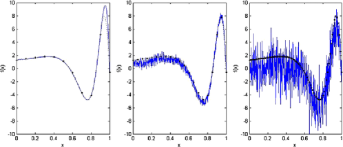
Figure 1: Panels 1–3: interpolator in solid blue and actual function in dotted black with collected data indicated by black dots.

Suppose that one is in the situation where most of the data sites are well spread, but a few poorly separated data sites are causing small numeric errors to be amplified. Consider forming an interpolator in two stages. In the first stage, remove the data sites which are causing the ill-conditioning of the interpolation matrix and interpolate the remaining points with a relatively wide kernel. The nominal error will be only slightly larger than the error for the full data set, since the removed data sites were nearly equal to data sites which were included. However, the numeric error will be substantially less than that of an interpolator formed on the full data set. In the second stage, interpolate the residuals from the first-stage interpolator using a kernel which is narrow enough that numeric errors remain small. The second-stage interpolator will increase neither the nominal accuracy nor the numeric error substantially. When the two interpolators are added together to form the multi-step interpolator, the nominal accuracy may be slightly worse, but the numeric accuracy will be very much better.

For example, consider building an emulator for the Michalewicz function

$$f(x,y)=\sin(\pi x)\sin^{20}(\pi x^{2})+\sin(\pi y)\sin^{20}(2\pi y^{2})$$

using the third 925 point data set in Figure 2 with separation distance $5\times 10^{-11}$.

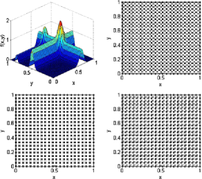
Figure 2: Panel 1: the Michalewicz function. Panels 2–4 in clockwise order: 925 point data sets with separation distances $0.017$, $0.009$ and $5\times 10^{-11}$, respectively.

The separation distance of a point set $X$ is half the distance between the closest two points,

$$q_{X}={\frac{1}{2}\min_{x_{i},x_{j}\in X}}\|x_{i}-x_{j}\|_{2}.$$ (10)

Clearly, the $\times$’s do not contribute much information about the unknown surface. If an ordinary Gaussian kernel interpolator, corresponding to a single stage with

$$\Phi(x-y)=\operatorname{exp}\Biggl{\{}-\sum_{j=1}^{2}\theta_{j}(x_{j}-y_{j})^{2}\Biggr{\}}$$ (11)

is built using all the data sites, the best possible mean squared prediction error over values of $\theta_{1},\theta_{2}$ is $\approx$$0.15$, the square of the function’s $L_{2}$ norm. This is because the kernel must be very narrow, or the interpolation matrix will be nearly singular. Throughout, the term mean squared prediction error is taken to be the average prediction error over the input domain. If, on the other hand, the $\bolds{\cdot}$’s are interpolated and then the residuals on the $\times$’s are interpolated, corresponding to two stages, the best possible mean squared prediction error over values of $\theta_{1},\theta_{2}$ at each stage is $\approx$$1.5\times 10^{-5}$.

4 Numeric accuracy

The numeric accuracy of the multi-step interpolation procedure depends on the accuracy of floating point matrix manipulations. Floating point accuracy refers to the fact that computers do not perform calculations with real numbers, but instead with rounded versions thereof. For example, a typical computer has 15 digits of accuracy meaning that

$$\frac{\|\tilde{x}-x\|_{2}}{\|x\|_{2}}\leq 10^{-15},$$

where $x$ denotes the actual value, and $\tilde{x}$ denotes the value that the computer stores.

4.1 Numeric accuracy of matrix inversion

The following lemma on the accuracy of floating point matrix inversion is a combination and generalization of results in golub .

Definition 2.

The matrix 2-norm $\|\cdot\|_{2}$ is defined as $\|A\|_{2}\,{=}\,\sqrt{\lambda_{\max}(A^{\prime}A)}$.

Lemma 1

Suppose $Ax=b$ and $\tilde{A}\tilde{x}=\tilde{b}$ with $\|A-\tilde{A}\|_{2}\leq\delta_{A}\|A\|_{2}$, $\|b-\tilde{b}\|_{2}\leq\delta_{b}\|b\|_{2}$ and $\kappa(A)=r/\delta_{A}<1/\delta_{A}$ for some $\delta_{A},\delta_{b}>0$. Then $\tilde{A}$ is nonsingular,

$$\frac{\|\tilde{x}\|_{2}}{\|x\|_{2}} \leq \frac{1+r(\delta_{b}/\delta_{A})}{1-r},$$

$$\frac{\|x-\tilde{x}\|_{2}}{\|x\|_{2}} \leq \frac{\delta_{A}+\delta_{b}}{1-r}\kappa(A),$$

where $\kappa(A)=\|A\|_{2}\|A^{-1}\|_{2}$.

Suppose $\tilde{A}$ is singular. Then there is a $y\neq 0$ with $\tilde{A}y=0$ so $(I-A^{-1}\tilde{A})y=y$. This implies $\|I-A^{-1}\tilde{A}\|_{2}\geq 1$. On the other hand, the conditions $\|A-\tilde{A}\|_{2}\leq\delta_{A}\|A\|_{2}$ and $\kappa(A)<1/\delta_{A}$ imply $\|I-A^{-1}\tilde{A}\|_{2}<1$ giving a contradiction.

Now, $\tilde{A}\tilde{x}=\tilde{b}$ implies $A^{-1}\tilde{A}\tilde{x}=A^{-1}(b-(b-\tilde{b}))=x+A^{-1}(\tilde{b}-b)$. The condition $\|I-A^{-1}\tilde{A}\|_{2}\leq r$ implies $\|A^{-1}\tilde{A}\|_{2}\geq 1-r$ and in turn

$$\|\tilde{x}\|_{2} \leq \frac{1}{1-r}(\|x\|_{2}+\|A^{-1}\|_{2}\|\tilde{b}-b\|_{2})$$

$$\leq \frac{1}{1-r}(\|x\|_{2}+\delta_{b}\|A^{-1}\|_{2}\|b\|_{2})$$

$$\leq \frac{1}{1-r}\biggl{(}\|x\|_{2}+r\frac{\delta_{b}\|b\|_{2}}{\delta_{A}\|A\|_{2}}\biggr{)}$$

$$\leq \frac{1}{1-r}\bigl{(}\|x\|_{2}+r(\delta_{b}/\delta_{A})\|x\|_{2}\bigr{)},$$

where the first inequality follows from the stated condition, the triangle inequality, and the fact that $\|By\|_{2}\leq\|B\|_{2}\|y\|_{2}$, the second inequality follows from the condition $\|b-\tilde{b}\|_{2}\leq\delta_{b}\|b\|_{2}$, the third inequality follows from the condition $\kappa(A)=r/\delta_{A}$ and the final inequality follows from $\|b\|_{2}\leq\|A\|_{2}\|x\|_{2}$. Dividing by $\|x\|_{2}$ gives the first inequality in (1).

Note that $A(\tilde{x}-x)=\tilde{b}-b-(\tilde{A}-A)\tilde{x}$. So,

$$\|\tilde{x}-x\|_{2} \leq \|A^{-1}\|_{2}\|\tilde{b}-b\|_{2}+\|A^{-1}\|_{2}\|\tilde{A}-A\|_{2}\|\tilde{x}\|_{2}$$

$$\leq \delta_{b}\|A^{-1}\|_{2}\|b\|_{2}+\delta_{A}\|A^{-1}\|_{2}\|A\|_{2}\|\tilde{x}\|_{2}$$

$$\leq \delta_{b}\kappa(A)\frac{\|b\|_{2}}{\|A\|_{2}}+\delta_{A}\kappa(A)\|\tilde{x}\|_{2}$$

$$\leq \kappa(A)\|x\|_{2}\biggl{(}\delta_{b}+\delta_{A}\frac{1+r(\delta_{b}/\delta_{A})}{1-r}\biggr{)},$$

where the first inequality follows from the triangle inequality and the fact that $\|By\|_{2}\leq\|B\|_{2}\|y\|_{2}$, the second inequality follows from the conditions $\|b-\tilde{b}\|_{2}\leq\delta_{b}\|b\|_{2}$ and $\|A-\tilde{A}\|_{2}\leq\delta_{A}\|A\|_{2}$, the third inequality follows from the definition of $\kappa(A)$ and the final inequality follows from the fact that $\|b\|_{2}\leq\|A\|_{2}\|x\|_{2}$ and the first inequality in (1). Dividing by $\|x\|_{2}$ and simplifying gives the second part of (1).

4.2 Numeric accuracy of single-stage interpolator

The above lemma can be used to bound the numeric error of an interpolator as follows.

Theorem 4.1.

Suppose that $\|A_{X,\Phi}-\tilde{A}_{X,\Phi}\|_{2}\leq\delta_{A}\|A_{X,\Phi}\|_{2}$, $\|f|_{X}-\break\tilde{f}|_{X}\|_{2}\leq\delta_{f}\|f|_{X}\|_{2}$, $\kappa(A_{X,\Phi})=r/\delta_{A}<1/\delta_{A}$ and $\sup_{x,y\in\Omega}|\Phi(x-y)-\tilde{\Phi}(x-y)|<D\delta_{A}$ for some $\delta_{A},\delta_{f},D>0$, then

$$|\mathcal{P}(x)-\tilde{\mathcal{P}}(x)| \leq \bigl{\|}f|_{X}/\sqrt{n}\bigr{\|}_{2}\frac{(\delta_{A}+\delta_{f})}{1-r}g(X,\Phi),$$

$$g(X,\Phi) = \frac{n}{\lambda_{\min}(A_{X,\Phi})}\bigl{(}\kappa(A_{X,\Phi})\Phi(0)+D\bigr{)},$$

where $\kappa(\cdot)$ is defined in Lemma 1.

Note that for large $n$ and approximately uniform $X$, $\|f|_{X}/\sqrt{n}\|_{2}\approx\|f\|_{L_{2}(\Omega)}$, where

$$\|f\|_{L_{2}(\Omega)}=\sqrt{\int_{\Omega}f(x)^{2}\,\mathrm{d}x}.$$

Further, the assumption ${\sup_{x,y\in\Omega}}|\Phi(x-y)-\tilde{\Phi}(x-y)|<D\delta_{A}$ requires that the kernel is computed in a relatively accurate manner. Proof of Theorem 4.1 First,

$$\mathcal{P}(x)-\tilde{\mathcal{P}}(x) = \sum_{i=1}^{n}[\alpha_{i}\Phi(x-x_{i})-\tilde{\alpha}_{i}\tilde{\Phi}(x-x_{i})]$$

$$= \sum_{i=1}^{n}\bigl{[}(\alpha_{i}-\tilde{\alpha}_{i})\Phi(x-x_{i})-\tilde{\alpha}_{i}\bigl{(}\tilde{\Phi}(x-x_{i})-\Phi(x-x_{i})\bigr{)}\bigr{]}.$$

So,

$$|\mathcal{P}(x)-\tilde{\mathcal{P}}(x)|$$

$$\qquad\leq\Biggl{|}\sum_{i=1}^{n}(\alpha_{i}-\tilde{\alpha}_{i})\Phi(x-x_{i})\Biggr{|}$$

$$\qquad\quad{}+\Biggl{|}\sum_{i=1}^{n}\tilde{\alpha}_{i}\bigl{(}\tilde{\Phi}(x-x_{i})-\Phi(x-x_{i})\bigr{)}\Biggr{|}.$$

Applying the Cauchy–Schwarz inequality to each term gives

$$|\mathcal{P}(x)-\tilde{\mathcal{P}}(x)|$$

$$\qquad\leq\|\alpha-\tilde{\alpha}\|_{2}\sqrt{\sum_{i=1}^{n}\Phi(x-x_{i})^{2}}$$

$$\qquad\quad{}+\|\tilde{\alpha}\|_{2}\sqrt{\sum_{i=1}^{n}\bigl{(}\tilde{\Phi}(x-x_{i})-\Phi(x-x_{i})\bigr{)}^{2}}.$$

The terms under the radicals can be bounded to obtain

$$|\mathcal{P}(x)-\tilde{\mathcal{P}}(x)|\leq\sqrt{n}\|\alpha-\tilde{\alpha}\|_{2}\Phi(0)+\sqrt{n}\|\tilde{\alpha}\|_{2}D\delta_{A}.$$

Now, Lemma 1 can be applied to the coefficients, giving

$$|\mathcal{P}(x)-\tilde{\mathcal{P}}(x)| \leq \sqrt{n}\frac{\delta_{A}+\delta_{f}}{1-r}\kappa(A_{X,\Phi})\|\alpha\|_{2}\Phi(0)$$

$${}+\sqrt{n}\frac{1+r(\delta_{f}/\delta_{A})}{1-r}\|\alpha\|_{2}D\delta_{A}.$$

Noting that $\|\alpha\|_{2}\leq\|A^{-1}_{X,\Phi}\|_{2}\|f|_{X}\|_{2}$ and collecting terms shows that

$$|\mathcal{P}(x)-\tilde{\mathcal{P}}(x)| \leq \frac{\sqrt{n}\|A^{-1}_{X,\Phi}\|_{2}\|f|_{X}\|_{2}}{1-r}$$

$${}\times\bigl{(}(\delta_{A}+\delta_{f})\kappa(A_{X,\Phi})\Phi(0)+D(\delta_{A}+r\delta_{f})\bigr{)}$$

$$\leq \frac{\sqrt{n}\|A^{-1}_{X,\Phi}\|_{2}\|f|_{X}\|_{2}}{1-r}(\delta_{A}+\delta_{f})\bigl{(}\kappa(A_{X,\Phi})\Phi(0)+D\bigr{)}.$$

Rearranging gives the result.

4.3 Numeric accuracy of multi-step interpolator

The first numeric result for the multi-step interpolator follows from Theorem 4.1. Here, $\delta$ denotes the computer’s floating point accuracy, typically $\delta\leq 10^{-15}$.

Theorem 4.2.

Suppose that for $j=1,\ldots,J$, $\|A_{X_{j},\Phi_{j}}-\tilde{A}_{X_{j},\Phi_{j}}\|_{2}\leq\break\delta_{j}\|A_{X_{j},\Phi_{j}}\|_{2}$, $\|f|_{X_{j}}-\tilde{f}|_{X_{j}}\|_{2}\leq\delta\|f|_{X_{j}}\|_{2}$, $\kappa(A_{X_{j},\Phi_{j}})\leq r/\delta_{j}<1/\delta_{j}$ and${\sup_{x,y\in\Omega}}|\Phi_{j}(x-y)-\tilde{\Phi}_{j}(x-y)|<D\delta$ for some $\delta_{j},\delta,D>0$ with $\delta_{j}\|(f-\sum_{k=1}^{j-1}\mathcal{P}^{k})|_{X_{j}}/\sqrt{n_{j}}\|_{2}\leq\delta\|f|_{X_{j}}/\sqrt{n_{j}}\|_{2}$, then

$$\Biggl{|}\sum_{j=1}^{J}\mathcal{P}^{j}(x)-\sum_{j=1}^{J}\tilde{\mathcal{P}}^{j}(x)\Biggr{|}$$

$$\qquad\leq\delta\bigl{\|}f|_{X_{J}}/\sqrt{n_{J}}\bigr{\|}_{2}\Biggl{[}\sum_{M=1}^{J}C^{M}\sum_{i\in\mathcal{S}_{J}(M)}\prod_{k=1}^{M}\rho(X_{i_{k}},X_{i_{k+1}})g(X_{i_{k}},\Phi_{i_{k}})\Biggr{]},$$

where $C=2/(1-r)$, $\mathcal{S}_{J}(M)=\{i\in\mathbb{N}^{M+1}\dvtx 1\leq i_{1}<\cdots<i_{M}\leq i_{M+1}=J\}$ $\rho(X,Y)=\|f|_{X}/\sqrt{n_{X}}\|_{2}/\|f|_{Y}/\sqrt{n_{Y}}\|_{2}$, and $g$ is defined in Theorem 4.1.

The assumption $\delta_{j}\|(f-\sum_{k=1}^{j-1}\mathcal{P}^{k})|_{X_{j}}/\sqrt{n_{j}}\|_{2}\leq\delta\|f|_{X_{j}}/\sqrt{n_{j}}\|_{2}$ roughly requires that the nominal errors either shrink or are not much larger than the function values. In practice, combinations of functions and training data sets which do not meet this assumption are very rare. Proof of Theorem 4.2 The result can be shown using induction on the number of stages $J$. If $J=1$, then the result follows immediately from Theorem 4.1. Take $J\geq 2$, and assume the result holds for $J-1$ stages. Then

$$\Biggl{\|}\Biggl{(}f-\sum_{j=1}^{J-1}\mathcal{P}^{j}\Biggr{)}\Bigg{|}_{X_{J}}-\Biggl{(}\tilde{f}-\sum_{j=1}^{J-1}\tilde{\mathcal{P}}^{j}\Biggr{)}\Bigg{|}_{X_{J}}\Biggr{\|}_{2}$$

$$\qquad\leq\bigl{\|}f|_{X_{J}}-\tilde{f}|_{X_{J}}\bigr{\|}_{2}+\Biggl{\|}\Biggl{(}\sum_{j=1}^{J-1}\mathcal{P}^{j}-\sum_{j=1}^{J-1}\tilde{\mathcal{P}}^{j}\Biggr{)}\Bigg{|}_{X_{J}}\Biggr{\|}_{2}$$ (14)

$$\qquad\leq\delta\|f|_{X_{J}}\|_{2}+\sqrt{n_{J}}\Biggl{\|}\sum_{j=1}^{J-1}\mathcal{P}^{j}-\sum_{j=1}^{J-1}\tilde{\mathcal{P}}^{j}\Biggr{\|}_{L_{\infty}(\Omega)},$$

where the first inequality follows from the triangle inequality, and the second inequality follows from the assumptions and by bounding the $L_{2}$ error with the maximum error. The induction hypothesis can be applied to the final term in (4.3) giving the bound

$$\delta\|f|_{X_{J}}\|_{2}$$

(15)

$$\quad{}\times\Biggl{(}1\,{+}\,\rho(X_{J-1},X_{J})\!\sum_{M=1}^{J-1}C^{M}\!\sum_{i\in\mathcal{S}_{J-1}(M)}\!\prod_{k=1}^{M}\!\rho(X_{i_{k}},X_{i_{k+1}})g(X_{i_{k}},\Phi_{i_{k}})\!\Biggr{)}.$$

In stage $J$, the error from the first $J-1$ stages are interpolated on $X_{J}$. After multiplying and dividing the above bound (4.3) by $\|(f-\sum_{j=1}^{J-1}\mathcal{P}^{j})|_{X_{J}}\|_{2}$, Theorem 4.1 can be used to bound the error due to stage $J$. Note that the term $\delta_{f}$ in Theorem 4.1 is the above bound (4.3) divided by $\|(f-\sum_{j=1}^{J-1}\mathcal{P}^{j})|_{X_{J}}\|_{2}$ and the term $\delta_{A}$ in Theorem 4.1 is $\delta_{j}$. By assumption, $\delta_{j}$ is smaller than or equal to (4.3) divided by $\|(f-\sum_{j=1}^{J-1}\mathcal{P}^{j})|_{X_{J}}\|_{2}$. Simplification and coarsening of the bound gives

$$|\mathcal{P}^{J}(x)-\tilde{\mathcal{P}}^{J}(x)|$$

$$\quad\leq\delta\bigl{\|}f|_{X_{J}}/\sqrt{n_{J}}\bigr{\|}_{2}\frac{2}{1-r}g(X_{J},\Phi_{J})$$ (16)

$$\qquad\times\Biggl{(}1\,{+}\,\rho(X_{J-1},X_{J})\!\sum_{M=1}^{J-1}C^{M}\!\sum_{i\in\mathcal{S}_{J-1}(M)}\!\prod_{k=1}^{M}\rho(X_{i_{k}},X_{i_{k+1}})g(X_{i_{k}},\Phi_{i_{k}})\!\Biggr{)}.$$

Now,

$$\Biggl{|}\sum_{j=1}^{J}\mathcal{P}^{j}(x)-\sum_{j=1}^{J}\tilde{\mathcal{P}}^{j}(x)\Biggr{|}\leq\Biggl{|}\sum_{j=1}^{J-1}\mathcal{P}^{j}(x)-\sum_{j=1}^{J-1}\tilde{\mathcal{P}}^{j}(x)\Biggr{|}+|\mathcal{P}^{J}(x)-\tilde{\mathcal{P}}^{J}(x)|.$$

So, the induction hypothesis can be applied again along with (4.3) giving

$$\Biggl{|}\sum_{j=1}^{J}\mathcal{P}^{j}(x)-\sum_{j=1}^{J}\tilde{\mathcal{P}}^{j}(x)\Biggr{|}$$

$$\qquad\leq\delta\bigl{\|}f|_{X_{J}}/\sqrt{n_{J}}\bigr{\|}_{2}$$

$$\qquad\quad{}\times\Biggl{[}\rho(X_{J-1},X_{J})\sum_{M=1}^{J-1}C^{M}\sum_{i\in\mathcal{S}_{J-1}(M)}\prod_{k=1}^{M}\rho(X_{i_{k}},X_{i_{k+1}})g(X_{i_{k}},\Phi_{i_{k}})$$

(17)

$$\qquad\quad\hskip 17.5pt{}+Cg(X_{J},\Phi_{J})$$

$$\qquad\quad\hskip 17.5pt{}+C\rho(X_{J-1},X_{J})g(X_{J},\Phi_{J})$$

$$\qquad\quad\hskip 68.2pt{}\times\sum_{M=1}^{J-1}C^{M}\sum_{i\in\mathcal{S}_{J-1}(M)}\prod_{k=1}^{M}\rho(X_{i_{k}},X_{i_{k+1}})g(X_{i_{k}},\Phi_{i_{k}})\Biggr{]}.$$

Note that the term in square brackets in (4.2) is the sum of the terms with $i_{M}<J$ and $i_{M}=J$ giving

$$\sum_{M=1}^{J}C^{M}\sum_{i\in\mathcal{S}_{J}(M)}\prod_{k=1}^{M}\rho(X_{i_{k}},X_{i_{k+1}})g(X_{i_{k}},\Phi_{i_{k}})$$

$$\qquad=\sum_{M=1}^{J-1}C^{M}\sum_{i\in\mathcal{S}_{J}(M),i_{M}<J}\prod_{k=1}^{M}\rho(X_{i_{k}},X_{i_{k+1}})g(X_{i_{k}},\Phi_{i_{k}})$$

$$\qquad\quad{}+\sum_{M=1}^{J}C^{M}\sum_{i\in\mathcal{S}_{J}(M),i_{M}=J}\prod_{k=1}^{M}\rho(X_{i_{k}},X_{i_{k+1}})g(X_{i_{k}},\Phi_{i_{k}})$$

$$\qquad=\rho(X_{J-1},X_{J})\sum_{M=1}^{J-1}C^{M}\sum_{i\in\mathcal{S}_{J-1}(M)}\prod_{k=1}^{M}\rho(X_{i_{k}},X_{i_{k+1}})g(X_{i_{k}},\Phi_{i_{k}})$$

$$\qquad\quad{}+Cg(X_{j},\Phi_{J})+\sum_{M=2}^{J}C^{M}\sum_{i\in\mathcal{S}_{J}(M),i_{M}=J}\prod_{k=1}^{M}\rho(X_{i_{k}},X_{i_{k+1}})g(X_{i_{k}},\Phi_{i_{k}}),$$

which is exactly the term in square brackets in (4.3), proving the result.

4.4 Dependence on separation distance

The terms

$$g(X_{j},\Phi_{j})=\frac{n_{j}}{\lambda_{\min}(A_{X_{j},\Phi_{j}})}\bigl{(}\kappa(A_{X_{j},\Phi_{j}})\Phi(0)+D\bigr{)}$$ (18)

from Theorem 4.2 can be computed, at least approximately. However, by bounding (18) in terms of the separation distance, as defined in (10), the role of the data sites and the kernel’s smoothness in the numeric accuracy are revealed. These results indicate that using poorly separated data or a wide kernel $\Phi$ with a rapidly decaying Fourier transform, implying more smoothness, has more potential to result in large numeric errors in interpolation. The Fourier transform can be defined as follows.

Definition 3.

For $f\in L_{1}(\mathbb{R}^{d})$ define the Fourier transform stein1971

$$\hat{f}(\omega)=(2\pi)^{-d/2}\int_{\mathbb{R}^{d}}f(x)e^{-i\omega^{\prime}x}\,\mathrm{d}x.$$

To generate the bound on (18), the following result from wendland2005 can be used.

Theorem 4.3.

Let $\varphi_{*}(M,\Phi)=\inf_{\|\omega\|_{2}\leq 2M}\hat{\Phi}(\omega)$. Then

$$\lambda_{\min}(A_{X,\Phi}) \geq C_{d}\varphi_{*}(M_{d}/q,\Phi)/q^{d},$$

$$M_{d} = 12\bigl{(}\pi\Gamma^{2}(d/2+1)/9\bigr{)}^{1/(d+1)},$$

$$C_{d} = (M_{d}/2^{3/2})^{d}/\bigl{(}2\Gamma(d/2+1)\bigr{)}$$

for any $q\leq q_{X}$, where $A_{X,\Phi}=\{\Phi(x_{i}-x_{j})\}$.

To bound $\lambda_{\max}(A_{X,\Phi})$ below, Gershgorin’s theorem varga can be used. Gershgorin’s theorem states that the largest eigenvalue of $A_{X,\Phi}$ has

$$|\lambda_{\max}(A_{X,\Phi})-\Phi(x_{j}-x_{j})|\leq\sum_{i=1,i\neq j}^{n}|\Phi(x_{i}-x_{j})|.$$

Rearranging and coarsening the bound gives

$$\lambda_{\max}(A_{X,\Phi})\leq n\Phi(0).$$ (19)

Theorem 4.3 and inequality (19) can be combined to obtain the following theorem bounding (18).

Theorem 4.4.

Under the assumptions in Theorem 4.2,

$$g(X_{j},\Phi_{j}) \leq \kappa_{\mathrm{upper}}(X_{j},\Phi_{j})\bigl{(}\kappa_{\mathrm{upper}}(X_{j},\Phi_{j})\Phi(0)+D\bigr{)},$$

$$\kappa_{\mathrm{upper}}(X_{j},\Phi_{j}) = \frac{n_{j}q^{d}_{X_{j}}}{C_{d}\varphi_{*}(M_{d}/q_{X_{j}},\Phi_{j})}.$$

The nested sequence $X_{1}\subset\cdots\subset X_{J}$ in (1) with large separation distance can be generated from nested space-filling designs qian20091 , qtw2009 , qa10 , qian20092 , haaland1 , which were originally developed for the purpose of conducting multi-fidelity computer experiments. Space-filling designs have shown particular merit in numerical integration stein1987 , Owen1992 , owen1994 , owen1997 , OWEN1997a , tang93 , loh96a , loh96b , loh08 , loh . Theorem 4.4 provides new insights into the use of such designs in interpolation.

5 Nominal accuracy

The results in this section indicate that the nominal error in interpolation converges to zero more quickly for wider, smoother kernels $\Phi$, although the constant involved in this rate changes. This is in direct opposition to the numeric error, which tends to be smaller for narrower, less smooth kernels. In fact, it will be seen that convergence of the nominal error of an arbitrarily fast rate can be achieved with an infinitely smooth kernel, such as the Gaussian in (11).

A re-scaling is introduced in the following definition.

Definition 4.

For a nonsingular $\Theta$, define $\Phi_{\Theta}(x)=\Phi(\Theta x)$.

5.1 Point-wise bound

Initially, consider a single stage with a fixed $\Phi$ which is re-scaled by a fixed $\Theta$. For a set of input sites $X$ of size $n$, define the cardinal basis functions

$$u_{i}(x) = \sum_{i=1}^{n}\beta_{i}\Phi_{\Theta}(x-x_{j}),$$

$$u_{i}(x_{j}) = \mathbh{1}_{\{i=j\}}$$

for $i,j=1,\ldots,n$. Then

$$\mathcal{P}(x)=\sum_{i=1}^{n}f(x_{i})u_{i}(x).$$

Since $f(x)=\langle f,\Phi_{\Theta}(\cdot-x)\rangle_{\mathcal{N}_{\Phi_{\Theta}}(\Omega)}$ if $f\in\mathcal{N}_{\Phi_{\Theta}}(\Omega)$,

$$f(x)-\mathcal{P}(x) = \langle f,\Phi_{\Theta}(\cdot-x)\rangle_{\mathcal{N}_{\Phi_{\Theta}}(\Omega)}-\sum_{i=1}^{n}u_{i}(x)\langle f,\Phi_{\Theta}(\cdot-x_{i})\rangle_{\mathcal{N}_{\Phi_{\Theta}}(\Omega)}$$

$$= \Biggl{\langle}f,\Phi_{\Theta}(\cdot-x)-\sum_{i=1}^{n}u_{i}(x)\Phi_{\Theta}(\cdot-x_{i})\Biggr{\rangle}_{\mathcal{N}_{\Phi_{\Theta}}(\Omega)}.$$

Now, the Cauchy–Schwarz inequality can be applied, giving the error bound

$$|f(x)-\mathcal{P}(x)|\leq\|f\|_{\mathcal{N}_{\Phi_{\Theta}}(\Omega)}\Biggl{\|}\Phi_{\Theta}(\cdot-x)-\sum_{i=1}^{n}u_{i}(x)\Phi_{\Theta}(\cdot-x_{i})\Biggr{\|}_{\mathcal{N}_{\Phi_{\Theta}}(\Omega)}.$$ (20)

The second term on the right-hand side of (20) is the so-called power function, $P_{\Phi_{\Theta},X}$. It can be shown wendland2005 that if the domain of interest $\Omega$ is bounded and convex, then

$$P^{2}_{\Phi_{\Theta},X}\leq C_{1}\|\Phi_{\Theta}-p\|_{L_{\infty}(B(0,C_{2}h_{X}))},$$

where $C_{1},C_{2}>0$ are constants which may depend on $\Omega$, $p$ is any multivariate polynomial, $B(a,b)=\{x\in\mathbb{R}^{d}\dvtx\|x-a\|_{2}<b\}$ and $h_{X}$ denotes the fill distance

$$h_{X}={\sup_{x\in\Omega}\min_{x_{u}\in X}}\|x-x_{u}\|_{2}.$$

Now, if $\Phi$ has $k$ continuous derivatives, $p$ can be taken to be the Taylor’s polynomial of $\Phi_{\Theta}$ of degree $k-1$. Then

$$\|\Phi_{\Theta}-p\|_{L_{\infty}(B(0,C_{2}h_{X}))}\leq C_{3}\|\Theta\|^{k}_{2}h^{k}_{X},$$

where $C_{3}$ is a constant which does not depend on $\Theta$. Combining the above development gives the following.

Theorem 5.1.

Suppose that $\Omega$ is bounded and convex, $\Phi$ satisfies Assumption 1 and has $k$ continuous derivatives and $\Theta$ is nonsingular. Then

$$|f(x)-\mathcal{P}(x)|\leq C_{\Phi}\|\Theta\|^{k/2}_{2}h^{k/2}_{X}\|f\|_{\mathcal{N}_{\Phi_{\Theta}}(\Omega)}.$$

5.2 Native space bound

First, write $\Phi_{\Theta}\ast\Phi_{\Theta}$ as

$$\Phi_{\Theta}\ast\Phi_{\Theta}(x-y)=\int_{\Omega}\Phi_{\Theta}(x-t)\Phi_{\Theta}(y-t)\,\mathrm{d}t.$$

Then, for $f\in\mathcal{N}_{\Phi_{\Theta}\ast\Phi_{\Theta}}(\Omega)$ and $x\in\Omega$, express $f$ in terms of the integral operator

$$f(x)=\int_{\Omega}u(y)\Phi_{\Theta}\ast\Phi_{\Theta}(x-y)\,\mathrm{d}y,$$

where $u\in L_{2}(\Omega)$. Combining these expressions gives

$$f(x) = \int_{\Omega}u(y)\int_{\Omega}\Phi_{\Theta}(y-t)\Phi_{\Theta}(x-t)\,\mathrm{d}t\,\mathrm{d}y$$

$$= \int_{\Omega}v(t)\Phi_{\Theta}(x-t)\,\mathrm{d}t,$$

where $v\in L_{2}(\Omega)$ is given by

$$v(t)=\int_{\Omega}u(y)\Phi_{\Theta}(y-t)\,\mathrm{d}y$$

for $t\in\Omega$. Then

$$\|f-\mathcal{P}\|^{2}_{\mathcal{N}_{\Phi_{\Theta}}(\Omega)} = \langle f-\mathcal{P},f\rangle_{\mathcal{N}_{\Phi_{\Theta}}(\Omega)}$$

$$= \langle f-\mathcal{P},v\rangle_{L_{2}(\Omega)}$$

$$\leq \|f-\mathcal{P}\|_{L_{2}(\Omega)}\|v\|_{L_{2}(\Omega)},$$

where the first equality follows from the orthogonality of the interpolator and its error with respect to the native space norm, the second equality follows from the properties of the integral operator and the inequality follows from the Cauchy–Schwarz inequality.

If $\Phi$ has $k$ continuous derivatives, then the first term on the right-hand side of inequality (5.2) can be bounded using Theorem 5.1 as

$$\|f-\mathcal{P}\|_{L_{2}(\Omega)} \leq \sqrt{\operatorname{vol}\Omega}\|f-\mathcal{P}\|_{L_{\infty}}(\Omega)$$

$$\leq C_{\Phi}\|\Theta\|^{k/2}_{2}h_{X}^{k/2}\|f-\mathcal{P}\|_{\mathcal{N}_{\Phi_{\Theta}}(\Omega)},$$

where the first inequality follows by relating the $L_{2}(\Omega)$ and $L_{\infty}(\Omega)$ norms, and the second inequality follows by applying Theorem 5.1 to $f-\mathcal{P}$. Plugging inequality (5.2) into inequality (5.2) and canceling a single $\|f-\mathcal{P}\|_{\mathcal{N}_{\Phi_{\Theta}}(\Omega)}$ term gives

$$\|f-\mathcal{P}\|_{\mathcal{N}_{\Phi_{\Theta}}(\Omega)}\leq C_{\Phi}\|\Theta\|^{k/2}_{2}h_{X}^{k/2}\|v\|_{L_{2}(\Omega)}.$$ (23)

Using the properties of the integral operator, the square of the second term on the right-hand side of inequality (23) can be expressed as

$$\|v\|^{2}_{L_{2}(\Omega)} = \int_{\Omega^{3}}u(x)u(y)\Phi_{\Theta}(y-t)\Phi_{\Theta}(x-t)\,\mathrm{d}x\,\mathrm{d}y\,\mathrm{d}t$$

$$= \|f\|^{2}_{\mathcal{N}_{\Phi_{\Theta}\ast\Phi_{\Theta}}(\Omega)}.$$

Combining inequality (23) and equality (5.2) gives the following theorem.

Theorem 5.2.

Under the assumptions of Theorem 5.1,

$$\|f-\mathcal{P}\|_{\mathcal{N}_{\Phi_{\Theta}}(\Omega)}\leq C_{\Phi}\|\Theta\|_{2}^{k/2}h_{X}^{k/2}\|f\|_{\mathcal{N}_{\Phi_{\Theta}\ast\Phi_{\Theta}}(\Omega)}.$$

To allow for individual re-scalings in different stages, we start with some notation. Define $\Psi_{k}$ recursively as

$$\Psi^{0} = \Phi,$$

$$\Psi^{k} = \Psi^{k-1}\ast\Psi^{k-1}$$

for $k\in\mathbb{N}$. For the kernel on step $j$, take

$$\Phi_{j}=\Psi^{J-j}_{\Theta_{j}}.$$ (26)

We now develop a bound on $\|\cdot\|_{\mathcal{N}_{\Phi_{j}\ast\Phi_{j}}(\Omega)}$ in terms of $\|\cdot\|_{\mathcal{N}_{\Phi_{j-1}}(\Omega)}$. The basic assumptions on the re-scaling matrices $\Theta_{j}$ in this section are that they are nonsingular and larger than the $\Theta_{j-1}$ in the sense that $\lambda_{\max}(\Theta^{\prime}_{j-1}\Theta_{j-1}\Xi^{\prime}_{j}\Xi_{j})\leq 1$, where $\Xi^{\prime}_{j}=\Theta_{j}^{-1}$.

In the case $\Omega=\mathbb{R}^{d}$, the native space $\mathcal{N}_{\Phi_{\Theta}}(\mathbb{R}^{d})$ has norm defined through the inner product

$$\langle f,g\rangle_{\mathcal{N}_{\Phi_{\Theta}}(\mathbb{R}^{d})}=(2\pi)^{-d/2}\int_{\mathbb{R}^{d}}\frac{\hat{f}(\omega)\overline{\hat{g}(\omega)}}{\hat{\Phi}_{\Theta}(\omega)}\,\mathrm{d}\omega,$$ (27)

where $\hat{f}$ and $\overline{\hat{g}}$ denote the Fourier transform and complex conjugate of the Fourier transform, respectively, of $f,g\in\mathcal{N}_{\Phi_{\Theta}}(\mathbb{R}^{d})$ wendland2005 . This explicit representation of the native space inner product can be used to relate the native space norms for convolutions and re-scalings. Hereafter, take $\infty>c_{2}\geq c_{1}>0$ and $\hat{\Upsilon}$ with

$$\omega^{\prime}\omega\leq\nu^{\prime}\nu\quad\Longrightarrow\quad\hat{\Upsilon}(\omega)\geq\hat{\Upsilon}(\nu),\qquad c_{1}\hat{\Upsilon}(\omega)\leq\hat{\Phi}(\omega)\leq c_{2}\hat{\Upsilon}(\omega).$$ (28)

Assumption 1 ensures that $c_{1}$, $c_{2}$ and $\hat{\Psi}$ satisfying (28) exist wendland2005 . The bounds to follow are tightest for $c_{2}-c_{1}$ as small as possible. Essentially, we want a radially decreasing envelop on the Fourier transform of the underlying kernel $\Phi$ to simplify development. Note that the Fourier transforms $\hat{\Phi}$ and $\hat{\Phi}_{\Theta}$ are related in the following manner:

$$\hat{\Phi}_{\Theta}(\omega) = (2\pi)^{-d/2}\int_{\mathbb{R}^{d}}\Phi_{\Theta}(x)e^{-i\omega^{\prime}x}\,\mathrm{d}x$$

$$= (2\pi)^{-d/2}\int_{\mathbb{R}^{d}}\Phi(\Theta x)e^{-i\omega^{\prime}\Xi^{\prime}\Theta x}\,\mathrm{d}x$$

$$= (2\pi)^{-d/2}|{\operatorname{det}}(\Xi)|\int_{\mathbb{R}^{d}}\Phi(y)e^{-i\omega^{\prime}\Xi^{\prime}y}\,\mathrm{d}y$$

$$= |{\operatorname{det}}(\Xi)|\hat{\Phi}(\Xi\omega),$$

where $\Xi^{\prime}=\Theta^{-1}$ and the third equality follows by making the substitution $y=\Theta x$.

Proposition 5.1.

If Assumption 1 is satisfied and $\Theta_{j-1},\Theta_{j}$ are nonsingular with respective inverses $\Xi^{\prime}_{j-1},\Xi^{\prime}_{j}$, then

$$\lambda_{\max}(\Theta^{\prime}_{j-1}\Theta_{j-1}\Xi^{\prime}_{j}\Xi_{j})\leq 1$$

(30)

$$\quad\Longrightarrow\quad\|f\|^{2}_{\mathcal{N}_{\Phi_{j}\ast\Phi_{j}}(\mathbb{R}^{d})}\leq\biggl{(}\frac{c_{2}}{c_{1}}\biggr{)}^{2^{J-(j-1)}}\frac{|{\operatorname{det}}(\Xi_{j-1})|}{|{\operatorname{det}}(\Xi_{j})|^{2}}\|f\|^{2}_{\mathcal{N}_{\Phi_{j-1}}(\mathbb{R}^{d})}$$

for $1\leq j\leq J$ where $c_{1}$ and $c_{2}$ satisfy (28), and $\Phi_{j-1}$ and $\Phi_{j}$ satisfy relations (5.2) and (26).

If $f\notin\mathcal{N}_{\Phi_{j-1}}(\mathbb{R}^{d})$, then $\|f\|^{2}_{\mathcal{N}_{\Phi_{j-1}}(\mathbb{R}^{d})}=\infty$ and (5.1) is true. Now, assume $f\in\mathcal{N}_{\Phi_{j-1}}(\mathbb{R}^{d})$, and note that

$$\frac{\omega^{\prime}\Xi^{\prime}_{j}\Xi_{j}\omega}{\omega^{\prime}\Xi^{\prime}_{j-1}\Xi_{j-1}\omega}\leq\lambda_{\max}(\Theta^{\prime}_{j-1}\Theta_{j-1}\Xi^{\prime}_{j}\Xi_{j}).$$

If $\lambda_{\max}(\Theta^{\prime}_{j-1}\Theta_{j-1}\Xi^{\prime}_{j}\Xi_{j})\leq 1$, then

$$\omega^{\prime}\Xi^{\prime}_{j}\Xi_{j}\omega\leq\omega^{\prime}\Xi^{\prime}_{j-1}\Xi_{j-1}\omega$$

$$\quad\Longrightarrow\quad\frac{1}{c_{1}}\hat{\Phi}(\Xi_{j}\omega)\geq\hat{\Upsilon}(\Xi_{j}\omega)\geq\hat{\Upsilon}(\Xi_{j-1}\omega)\geq\frac{1}{c_{2}}\hat{\Phi}(\Xi_{j-1}\omega)$$

(31)

$$\quad\Longrightarrow\quad\frac{1}{\hat{\Phi}(\Xi_{j}\omega)^{2^{J-j}}}\leq\biggl{(}\frac{c_{2}}{c_{1}}\biggr{)}^{2^{J-j}}\frac{1}{\hat{\Phi}(\Xi_{j-1}\omega)^{2^{J-j}}}$$

$$\quad\Longrightarrow\quad\frac{1}{\hat{\Psi}^{J-j}(\Xi_{j}\omega)}\leq\biggl{(}\frac{c_{2}}{c_{1}}\biggr{)}^{2^{J-j}}\frac{1}{\hat{\Psi}^{J-j}(\Xi_{j-1}\omega)},$$

where the first implication follows from (28), the second implication follows since the right- and left-hand sides are positive and the final implication follows from the relations (5.2) and (26) and the properties of Fourier transforms of convolutions. So,

$$\|f\|^{2}_{\mathcal{N}_{\Phi_{j-1}}(\mathbb{R}^{d})}$$

$$\qquad=\|f\|^{2}_{\mathcal{N}_{\Psi^{J-(j-1)}_{\Theta_{j-1}}}(\mathbb{R}^{d})}$$

$$\qquad=(2\pi)^{-d/2}\int_{\mathbb{R}^{d}}\frac{|\hat{f}(\omega)|^{2}}{\hat{\Psi}^{J-(j-1)}_{\Theta_{j-1}}(\omega)}\,\mathrm{d}\omega$$

$$\qquad=\frac{(2\pi)^{-d/2}}{|{\operatorname{det}}(\Xi_{j-1})|}\int_{\mathbb{R}^{d}}\frac{|\hat{f}(\omega)|^{2}}{\hat{\Psi}^{J-(j-1)}(\Xi_{j-1}\omega)}\,\mathrm{d}\omega$$

$$\qquad=\frac{(2\pi)^{-d/2}}{|{\operatorname{det}}(\Xi_{j-1})|}\int_{\mathbb{R}^{d}}\frac{|\hat{f}(\omega)|^{2}}{\widehat{\Psi^{J-j}\ast\Psi^{J-j}}(\Xi_{j-1}\omega)}\,\mathrm{d}\omega$$

$$\qquad=\frac{(2\pi)^{-d}}{|{\operatorname{det}}(\Xi_{j-1})|}\int_{\mathbb{R}^{d}}\frac{|\hat{f}(\omega)|^{2}}{\hat{\Psi}^{J-j}(\Xi_{j-1}\omega)^{2}}\,\mathrm{d}\omega$$

$$\qquad=(2\pi)^{-d}\frac{|{\operatorname{det}}(\Xi_{j})|^{2}}{|{\operatorname{det}}(\Xi_{j-1})|}\int_{\mathbb{R}^{d}}\frac{|\hat{f}(\omega)|^{2}}{|{\operatorname{det}}(\Xi_{j})|^{2}\hat{\Psi}^{J-j}(\Xi_{j-1}\omega)^{2}}\,\mathrm{d}\omega$$

$$\qquad\geq(2\pi)^{-d}\frac{|{\operatorname{det}}(\Xi_{j})|^{2}}{|{\operatorname{det}}(\Xi_{j-1})|}\biggl{(}\frac{c_{1}}{c_{2}}\biggr{)}^{2^{J-j+1}}\int_{\mathbb{R}^{d}}\frac{|\hat{f}(\omega)|^{2}}{|{\operatorname{det}}(\Xi_{j})|^{2}\hat{\Psi}^{J-j}(\Xi_{j}\omega)^{2}}\,\mathrm{d}\omega$$

$$\qquad=(2\pi)^{-d/2}\frac{|{\operatorname{det}}(\Xi_{j})|^{2}}{|{\operatorname{det}}(\Xi_{j-1})|}\biggl{(}\frac{c_{1}}{c_{2}}\biggr{)}^{2^{J-j+1}}\int_{\mathbb{R}^{d}}\frac{|\hat{f}(\omega)|^{2}}{\widehat{\Psi^{J-j}_{\Theta_{j}}\ast\Psi^{J-j}_{\Theta_{j}}}(\omega)}\,\mathrm{d}\omega$$

$$\qquad=\frac{|{\operatorname{det}}(\Xi_{j})|^{2}}{|{\operatorname{det}}(\Xi_{j-1})|}\biggl{(}\frac{c_{1}}{c_{2}}\biggr{)}^{2^{J-j+1}}\|f\|^{2}_{\mathcal{N}_{\Phi_{j}\ast\Phi_{j}}(\mathbb{R}^{d})},$$

where the first equality follows from relation (26), the second equality follows from the inner product representation (27), the third equality follows from the scaled Fourier transform relation (5.2), the fourth equality follows from the definition of $\Psi^{J-(j-1)}$ (5.2), the fifth equality follows from the properties of Fourier transforms of convolutions, the sixth equality follows by multiplying by $|{\operatorname{det}}(\Xi_{j})|^{2}/|{\operatorname{det}}(\Xi_{j})|^{2}$, the inequality follows from the development (5.2), the seventh equality follows from the scaled Fourier transform relation (5.2) and the properties of Fourier transforms of convolutions and the final equality follows from the inner product representation (27).

In most applications, the domain of interest $\Omega$ is a strict subset of $\mathbb{R}^{d}$. If $f\in\mathcal{N}_{\Phi_{1}}(\Omega)$, then $f$ can be extended to $Ef\in\mathcal{N}_{\Phi_{1}}(\mathbb{R}^{d})$ wendland2005 with

$$\|f\|_{\mathcal{N}_{\Phi_{1}}(\Omega)} = \|Ef\|_{\mathcal{N}_{\Phi_{1}}(\mathbb{R}^{d})},$$

$$\|f\|_{\mathcal{N}_{\Phi_{2}}(\Omega)} \leq \|Ef\|_{\mathcal{N}_{\Phi_{2}}(\mathbb{R}^{d})}$$

for all $\Phi_{2}$. Combining (5.2) with Proposition 5.1 gives the following corollary.

Corollary 1

If the assumptions of Proposition 5.1 are satisfied, then

$$\lambda_{\max}(\Theta^{\prime}_{j-1}\Theta_{j-1}\Xi^{\prime}_{j}\Xi_{j})\leq 1$$

(33)

$$\quad\Longrightarrow\quad\|f\|^{2}_{\mathcal{N}_{\Phi_{j}\ast\Phi_{j}}(\Omega)}\leq\biggl{(}\frac{c_{2}}{c_{1}}\biggr{)}^{2^{J-(j-1)}}\frac{|{\operatorname{det}}(\Xi_{j-1})|}{|{\operatorname{det}}(\Xi_{j})|^{2}}\|f\|^{2}_{\mathcal{N}_{\Phi_{j-1}}(\Omega)}.$$

If $f\notin\mathcal{N}_{\Phi_{j-1}}(\Omega)$, then $\|f\|^{2}_{\mathcal{N}_{\Phi_{j-1}}(\Omega)}=\infty$ and (1) is true. Now, assume $f\in\mathcal{N}_{\Phi_{j-1}}(\Omega)$ and extend $f$ to $Ef\in\mathcal{N}_{\Phi_{j-1}}(\mathbb{R}^{d})$ with $\|Ef\|^{2}_{\mathcal{N}_{\Phi_{j-1}}(\mathbb{R}^{d})}=\|f\|^{2}_{\mathcal{N}_{\Phi_{j-1}}(\Omega)}$. Then

$$\|f\|^{2}_{\mathcal{N}_{\Phi_{j}\ast\Phi_{j}}(\Omega)} \leq \|Ef\|^{2}_{\mathcal{N}_{\Phi_{j}\ast\Phi_{j}}(\mathbb{R}^{d})}$$

$$\leq \biggl{(}\frac{c_{2}}{c_{1}}\biggr{)}^{2^{J-(j-1)}}\frac{|{\operatorname{det}}(\Xi_{j-1})|}{|{\operatorname{det}}(\Xi_{j})|^{2}}\|Ef\|^{2}_{\mathcal{N}_{\Phi_{j-1}}(\mathbb{R}^{d})}$$

$$= \biggl{(}\frac{c_{2}}{c_{1}}\biggr{)}^{2^{J-(j-1)}}\frac{|{\operatorname{det}}(\Xi_{j-1})|}{|{\operatorname{det}}(\Xi_{j})|^{2}}\|f\|^{2}_{\mathcal{N}_{\Phi_{j-1}}(\Omega)},$$

where the first inequality follows from (5.2), the second inequality follows from Proposition 5.1 and the equality follows from the property of the chosen extension.

5.3 Error bound for multi-step interpolator

Combining Theorem 5.2 with Corollary 1, we are able to obtain the following theorem bounding the native space norm of the multi-step interpolator’s error.

Theorem 5.3.

Under the assumptions of Theorem 5.1 and Proposition 5.1,

$$\Biggl{\|}f-\sum_{j=1}^{J}\mathcal{P}^{j}\Biggr{\|}_{\mathcal{N}_{\Phi_{J}}(\Omega)}\leq C_{\Phi,J}\|f\|_{\mathcal{N}_{\Phi_{0}}(\Omega)}\prod_{j=1}^{J}\biggl{\{}\frac{\sqrt{|{\operatorname{det}}(\Xi_{j-1})|}}{|{\operatorname{det}}(\Xi_{j})|}(\|\Theta_{j}\|^{k}_{2}h^{k}_{X_{j}})^{2^{J-j-1}}\biggr{\}}.$$

First applying Theorem 5.2 and then applying Proposition 5.1 gives

$$\Biggl{\|}f-\sum_{j=1}^{J}\mathcal{P}^{j}\Biggr{\|}_{\mathcal{N}_{\Phi_{J}}(\Omega)} \leq C_{\Phi}\|\Theta_{J}\|_{2}^{k/2}h_{X_{J}}^{k/2}\Biggl{\|}f-\sum_{j=1}^{J-1}\mathcal{P}^{j}\Biggr{\|}_{\mathcal{N}_{\Phi_{J}\ast\Phi_{J}}(\Omega)}$$

$$\leq C_{\Phi,J}\|\Theta_{J}\|_{2}^{k/2}h_{X_{J}}^{k/2}\frac{\sqrt{|{\operatorname{det}}(\Xi_{J-1})|}}{|{\operatorname{det}}(\Xi_{J})|}\Biggl{\|}f-\sum_{j=1}^{J-1}\mathcal{P}^{j}\Biggr{\|}_{\mathcal{N}_{\Phi_{J-1}}(\Omega)}.$$

For $J\geq 2$, repeat the above argument $J-1$ more times, and note that $\Phi_{J-j}$ has $k2^{j}$ continuous derivatives.

By applying Theorem 5.1 to the error $f-\sum_{j=1}^{J}\mathcal{P}^{j}$, an additional multiple of $h_{X_{J}}^{k/2}$ is obtained in the following theorem.

Theorem 5.4.

Under the assumptions of Theorem 5.1 and Proposition 5.1,

$$\Biggl{|}f(x)-\sum_{j=1}^{J}\mathcal{P}^{j}(x)\Biggr{|}$$

$$\qquad\leq C_{\Phi,J}\|f\|_{\mathcal{N}_{\Phi_{0}}(\Omega)}\|\Theta_{J}\|_{2}^{k/2}h_{X_{J}}^{k/2}\prod_{j=1}^{J}\biggl{\{}\frac{\sqrt{|{\operatorname{det}}(\Xi_{j-1})|}}{|{\operatorname{det}}(\Xi_{j})|}(\|\Theta_{j}\|^{k}_{2}h^{k}_{X_{j}})^{2^{J-j-1}}\biggr{\}}.$$

6 Examples

First, consider using the multi-step procedure to interpolate Franke’s function

$$f(x,y) = \tfrac{3}{4}\operatorname{exp}\bigl{\{}-\bigl{(}(9x-2)^{2}+(9y-2)^{2}\bigr{)}/4\bigr{\}}$$

$${}+\tfrac{3}{4}\operatorname{exp}\bigl{\{}-\bigl{(}(9x+1)^{2}/49-(9y+1)^{2}/10\bigr{)}\bigr{\}}$$

$${}+\tfrac{1}{2}\operatorname{exp}\bigl{\{}-\bigl{(}(9x-7)^{2}+(9y-3)^{2}\bigr{)}/4\bigr{\}}$$

$${}-\tfrac{1}{5}\operatorname{exp}\bigl{\{}-\bigl{(}(9x-4)^{2}+(9y-7)^{2}\bigr{)}\bigr{\}}$$

shown in the left panel of Figure 3. Theorems 4.2 and 4.4 indicate that each of the nested data sets should have well-separated points in the full

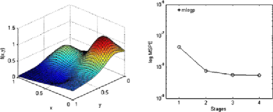
Figure 3: Left panel: Franke’s function. Right panel: log mean squared prediction error versus number of stages (circles) and using mlegp (asterisk).

dimension as well as lower-dimensional projections to give small numeric error, and Theorem 5.4 indicates that each of the nested data sets should have small data-free regions in the full dimension as well as lower-dimensional projections to give small nominal error. Training data are collected from Franke’s function using a randomized $(0,4,2)$-net in base 5 owen1995 with $5^{4}=625$ points, which has a convenient nested structure with both the full and each sub-design having small data-free regions and relatively well-spread points in both the full and projected space, making it ideal for the multi-step procedure. Theorem 4.4 indicates that a less smooth underlying kernel $\Phi$ will give more numerically accurate results, while Theorem 5.4 indicates that a more smooth kernel will give more nominally accurate results. To balance these opposing forces in this moderately sized example, the selected $\Phi$ is Wendland’s compactly supported kernel with four continuous derivatives wendland2005 ,

$$\Phi(x-y) = \phi\bigl{(}\sqrt{(x-y)^{\prime}(x-y)}\bigr{)},$$

$$\phi(r) = (1-r)^{l+2}_{+}[(l^{2}+4l+3)r^{2}+(3l+6)r+3],\qquad l=\lfloor d/2\rfloor+3,$$

and the rescaling matrices $\Theta_{1},\ldots,\Theta_{J}$ are restricted to be diagonal, so each input is re-scaled separately. The re-scalings for each stage are chosen by leave-one-out cross-validation, for which a simple short-cut formula holds making computation undemanding for this moderately sized problem, although $A^{-1}_{X_{j},\Phi_{j}}$ needs to be calculated. In particular, the $i$th cross-validation error at stage $j$ is rippa

$$e_{(i)}=\frac{\alpha^{j}_{i}}{B^{j}_{ii}},\qquad B^{j}=A^{-1}_{X_{j},\Phi_{j}}.$$ (34)

In this example, the single-stage sample size is $n_{1}=625$, the two-stage sample sizes are $n_{1}=250$ and $n_{2}=625$, the three-stage sample sizes are $n_{1}=250$, $n_{2}=375$ and $n_{3}=625$ and the four-stage sample sizes are $n_{1}=250$, $n_{2}=375$, $n_{3}=500$ and $n_{4}=625$. The nested data sets are $X_{j}=\{x_{i}\in X\dvtx i\leq n_{j}\}$. The right panel of Figure 3 shows the logarithm of the mean squared prediction error on a test set of 1,000 randomly generated uniform points. Notice that the mean squared prediction error is improved from $4.4\times 10^{-8}$ to $5.4\times 10^{-9}$. A Gaussian process fit using the mlegp package mlegp in R, on the other hand, has mean squared prediction error $6.8\times 10^{-7}$.

Next, consider using the multi-step procedure to interpolate Schwefel’s function for $d=5$

$$f(x)=-\sum_{j=1}^{d}(1\mbox{,}000x_{j}-500)\sin\bigl{(}\sqrt{|1\mbox{,}000x_{j}-500|}\bigr{)}/1\mbox{,}000,$$

a two-dimensional projection of which with the remaining variables fixed at $1/2$ is shown in the left panel of Figure 4. This function is relatively complex and a very large training set is needed to build an accurate emulator.

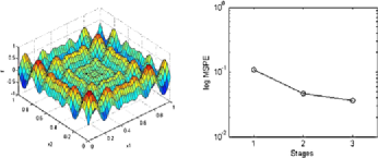
Figure 4: Left panel: two-dimensional projection of Schwefel’s function. Right panel: log mean squared prediction error versus number of stages.

To ensure easy nesting and good space-filling properties for sub-designs, data are collected from Schwefel’s function using a randomized $(0,8,5)$-net in base 5 with $5^{8}=390\mbox{,}625$ points. In this example there is a great deal of potential for numeric problems so Wendland’s continuous, compactly supported kernel,

$$\Phi(x-y) = \phi\bigl{(}\sqrt{(x-y)^{\prime}(x-y)}\bigr{)},$$

$$\phi(r) = (1-r)^{l+2}_{+},\qquad l=\lfloor d/2\rfloor+1$$

with relatively little smoothness is selected. The re-scaling matrices $\Theta_{1},\ldots,\allowbreak\Theta_{J}$ are chosen to be fixed scalar multiples of the identity, $\Theta_{j}=\theta_{j}I_{d}$, with

$$\theta_{j}=\biggl{(}\frac{n_{j}^{2}\pi^{d/2}}{10^{7}\Gamma(d/2+1)}\biggr{)}^{1/d},$$ (35)

which ensures that each intepolation matrix $A_{X_{j},\Phi_{j}}$ has less than $10^{7}$ nonzero entries. Edge effects in the five-dimensional cube ensure that the number of nonzero entries is substantially less than $10^{7}$. In this example, the single-stage sample size is $n_{1}=390\mbox{,}625$, the two-stage sample sizes are $n_{1}=5^{7}=78\mbox{,}125$ and $n_{2}=390\mbox{,}625$ and the three-stage sample sizes are $n_{1}=78\mbox{,}125$, $n_{2}=2\times 5^{7}=156\mbox{,}250$ and $n_{3}=390\mbox{,}625$. The nested data sets are $X_{j}=\{x_{i}\in X\dvtx i\leq n_{j}\}$. The right panel of Figure 4 shows the logarithm of the mean squared prediction error on a test set of 10,000 randomly generated uniform points. Notice that the mean squared prediction error is improved from $0.11$ to $0.036$. On the other hand, the mlegp package runs out of memory trying to fit a GP.

7 Discussion

We have presented the intuitively appealing and practically useful multi-step interpolation procedure. This procedure is easy to use and offers substantial improvements in overall accuracy in the emulation of large-scale computer experiments. We introduced a decomposition of the error of any interpolator into nominal and numeric portions. This decomposition is important because it allows the two sources of error to be analyzed separately while emphasizing the interplay between the two types of errors. We proved a very general result bounding the numeric error of a multi-step interpolator, of which an ordinary interpolator is a special case. This result constitutes the only complete and rigorous bound on the numeric error of the multi-step interpolator. We proved that in the situation where the earlier stage kernels are convolutions of the later stage kernels, substantial nominal improvements can be realized. In the context of the multi-step interpolator, this result is the most general and explicit of its kind.

Further work on the multi-step interpolation method will be explored in the following directions. First, its implementation details, along with various examples, will be reported in a subsequent article, to illustrate the theoretical results derived here. The implementation of the method requires the generation of nested data sites, for which the typical choice in applied mathematics is nested grids. Nested space-filling designs qian20091 , qa10 , qian20092 , haaland1 , originally constructed for running multiple computer experiments with different levels of accuracy, are a better choice because of their good uniformity properties. Such designs can be generated by exploiting nesting in orthogonal arrays HedayatSloaneStufken1999 , U designs tang93 , tang94 , orthogonal Latin hypercubes ye1998 , sl06 , bst09 , lin09 , lin10 or scrambled nets owen1995 . Second, emulation of computer models with qualitative and quantitative factors is currently getting increasing attention qww08 , qian20094 , han . We plan to extend the multi-step procedure to accommodate these two types of factors. Third, beyond emulation of computer experiments, singularity issues arise in fitting many other large kernel models. We plan to introduce a general multi-step framework for fitting kernel based classification and regression methods with a large number of observations. As in the multi-step interpolation procedure, this framework obtains nested data sites and then fits a kernel model in multiple steps, where in each step interpolation is replaced by an appropriate procedure for the given problem. New theoretical bounds on the nominal and numeric accuracy, analogous to those in Sections 4 and 5, will be derived for this framework. The required well-spread nested data sites for the framework will be generated by using nested space-filling designs or the efficient thinning algorithm floater for observational data. In the revision of this paper, we became aware of new theoretical developments of the multi-step method in applied mathematics, including GiSlWe10 and Wen10 .

References

- (1) {barticle}[mr] \bauthor\bsnmAronszajn, \bfnmN.\binitsN. (\byear1950). \btitleTheory of reproducing kernels. \bjournalTrans. Amer. Math. Soc. \bvolume68 \bpages337–404. \bidissn=0002-9947, mr=0051437 \bptokimsref \endbibitem
- (2) {barticle}[mr] \bauthor\bsnmBarry, \bfnmRonald Paul\binitsR. P. and \bauthor\bsnmPace, \bfnmR. Kelley\binitsR. K. (\byear1999). \btitleMonte Carlo estimates of the log determinant of large sparse matrices. \bjournalLinear Algebra Appl. \bvolume289 \bpages41–54. \biddoi=10.1016/S0024-3795(97)10009-X, issn=0024-3795, mr=1670972 \bptokimsref \endbibitem
- (3) {barticle}[mr] \bauthor\bsnmBingham, \bfnmDerek\binitsD., \bauthor\bsnmSitter, \bfnmRandy R.\binitsR. R. and \bauthor\bsnmTang, \bfnmBoxin\binitsB. (\byear2009). \btitleOrthogonal and nearly orthogonal designs for computer experiments. \bjournalBiometrika \bvolume96 \bpages51–65. \biddoi=10.1093/biomet/asn057, issn=0006-3444, mr=2482134 \bptokimsref \endbibitem
- (4) {bmisc}[auto:STB—2011/11/09—09:54:39] \borganizationThe Boeing Company (\byear2010). \bhowpublishedDesign space exploration software. \bptokimsref \endbibitem
- (5) {bmisc}[auto:STB—2011/11/09—09:54:39] \bauthor\bsnmBooker, \bfnmA. J.\binitsA. J. (\byear2000). \bhowpublishedWell-conditioned kriging models for optimization of computer simulations. Mathematics and Computing Technology Phantom Works, M&CT Technical Report 00-002, The Boeing Co., Bellvue, WA. \bptokimsref \endbibitem
- (6) {barticle}[mr] \bauthor\bsnmCurrin, \bfnmCarla\binitsC., \bauthor\bsnmMitchell, \bfnmToby\binitsT., \bauthor\bsnmMorris, \bfnmMax\binitsM. and \bauthor\bsnmYlvisaker, \bfnmDon\binitsD. (\byear1991). \btitleBayesian prediction of deterministic functions, with applications to the design and analysis of computer experiments. \bjournalJ. Amer. Statist. Assoc. \bvolume86 \bpages953–963. \bidissn=0162-1459, mr=1146343 \bptokimsref \endbibitem
- (7) {bmisc}[auto:STB—2011/11/09—09:54:39] \bauthor\bsnmDancik, \bfnmG. M.\binitsG. M. (\byear2011). \bhowpublishedmlegp: Maximum likelihood estimates of Gaussian processes. R package Version 3.1.2. Available at http://CRAN.R-project.org/package= mlegp. \bptokimsref \endbibitem
- (8) {bbook}[mr] \bauthor\bsnmFang, \bfnmKai-Tai\binitsK.-T., \bauthor\bsnmLi, \bfnmRunze\binitsR. and \bauthor\bsnmSudjianto, \bfnmAgus\binitsA. (\byear2006). \btitleDesign and Modeling for Computer Experiments. \bpublisherChapman and Hall/CRC, \baddressBoca Raton, FL. \bidmr=2223960 \bptokimsref \endbibitem
- (9) {barticle}[mr] \bauthor\bsnmFang, \bfnmKai-Tai\binitsK.-T., \bauthor\bsnmLin, \bfnmDennis K. J.\binitsD. K. J., \bauthor\bsnmWinker, \bfnmPeter\binitsP. and \bauthor\bsnmZhang, \bfnmYong\binitsY. (\byear2000). \btitleUniform design: Theory and application. \bjournalTechnometrics \bvolume42 \bpages237–248. \bidissn=0040-1706, mr=1801031 \bptokimsref \endbibitem
- (10) {bbook}[mr] \bauthor\bsnmFasshauer, \bfnmGregory E.\binitsG. E. (\byear2007). \btitleMeshfree Approximation Methods with MATLAB. \bseriesInterdisciplinary Mathematical Sciences \bvolume6. \bpublisherWorld Scientific, \baddressHackensack, NJ. \bidmr=2357267 \bptokimsref \endbibitem
- (11) {barticle}[mr] \bauthor\bsnmFasshauer, \bfnmGregory E.\binitsG. E. and \bauthor\bsnmJerome, \bfnmJoseph W.\binitsJ. W. (\byear1999). \btitleMultistep approximation algorithms: Improved convergence rates through postconditioning with smoothing kernels. \bjournalAdv. Comput. Math. \bvolume10 \bpages1–27. \biddoi=10.1023/A:1018962112170, issn=1019-7168, mr=1671863 \bptokimsref \endbibitem
- (12) {barticle}[mr] \bauthor\bsnmFloater, \bfnmMichael S.\binitsM. S. and \bauthor\bsnmIske, \bfnmArmin\binitsA. (\byear1996). \btitleMultistep scattered data interpolation using compactly supported radial basis functions. \bjournalJ. Comput. Appl. Math. \bvolume73 \bpages65–78. \biddoi=10.1016/0377-0427(96)00035-0, issn=0377-0427, mr=1424869 \bptokimsref \endbibitem
- (13) {barticle}[mr] \bauthor\bsnmGneiting, \bfnmTilmann\binitsT. (\byear2002). \btitleCompactly supported correlation functions. \bjournalJ. Multivariate Anal. \bvolume83 \bpages493–508. \biddoi=10.1006/jmva.2001.2056, issn=0047-259X, mr=1945966 \bptokimsref \endbibitem
- (14) {bbook}[mr] \bauthor\bsnmGolub, \bfnmGene H.\binitsG. H. and \bauthor\bsnmVan Loan, \bfnmCharles F.\binitsC. F. (\byear1989). \btitleMatrix Computations, \bedition2nd ed. \bseriesJohns Hopkins Series in the Mathematical Sciences \bvolume3. \bpublisherJohns Hopkins Univ. Press, \baddressBaltimore, MD. \bidmr=1002570 \bptokimsref \endbibitem
- (15) {barticle}[mr] \bauthor\bsnmHaaland, \bfnmBen\binitsB. and \bauthor\bsnmQian, \bfnmPeter Z. G.\binitsP. Z. G. (\byear2010). \btitleAn approach to constructing nested space-filling designs for multi-fidelity computer experiments. \bjournalStatist. Sinica \bvolume20 \bpages1063–1075. \bidissn=1017-0405, mr=2729853 \bptokimsref \endbibitem
- (16) {barticle}[mr] \bauthor\bsnmHales, \bfnmS. J.\binitsS. J. and \bauthor\bsnmLevesley, \bfnmJ.\binitsJ. (\byear2002). \btitleError estimates for multilevel approximation using polyharmonic splines. \bjournalNumer. Algorithms \bvolume30 \bpages1–10. \bptokimsref \endbibitem
- (17) {barticle}[mr] \bauthor\bsnmHan, \bfnmGang\binitsG., \bauthor\bsnmSantner, \bfnmThomas J.\binitsT. J., \bauthor\bsnmNotz, \bfnmWilliam I.\binitsW. I. and \bauthor\bsnmBartel, \bfnmDonald L.\binitsD. L. (\byear2009). \btitlePrediction for computer experiments having quantitative and qualitative input variables. \bjournalTechnometrics \bvolume51 \bpages278–288. \biddoi=10.1198/tech.2009.07132, issn=0040-1706, mr=2751072 \bptokimsref \endbibitem
- (18) {bbook}[auto:STB—2011/11/09—09:54:39] \bauthor\bsnmHarville, \bfnmD. A.\binitsD. A. (\byear2008). \btitleMatrix Algebra From a Statistician’s Perspective. \bpublisherSpringer, \baddressNew York. \bptokimsref \endbibitem
- (19) {bbook}[mr] \bauthor\bsnmHedayat, \bfnmA. S.\binitsA. S., \bauthor\bsnmSloane, \bfnmN. J. A.\binitsN. J. A. and \bauthor\bsnmStufken, \bfnmJohn\binitsJ. (\byear1999). \btitleOrthogonal Arrays: Theory and Applications. \bpublisherSpringer, \baddressNew York. \bidmr=1693498 \bptokimsref \endbibitem
- (20) {bmisc}[auto:STB—2011/11/09—09:54:39] \borganizationIBM (\byear2010). \bhowpublishedA smarter planet project. Available at http://www.ibm.com/ smarterplanet/. \bptokimsref \endbibitem
- (21) {barticle}[mr] \bauthor\bsnmJoseph, \bfnmV. Roshan\binitsV. R. and \bauthor\bsnmHung, \bfnmYing\binitsY. (\byear2008). \btitleOrthogonal-maximin Latin hypercube designs. \bjournalStatist. Sinica \bvolume18 \bpages171–186. \bidissn=1017-0405, mr=2416907 \bptokimsref \endbibitem
- (22) {barticle}[mr] \bauthor\bsnmKaufman, \bfnmCari G.\binitsC. G., \bauthor\bsnmSchervish, \bfnmMark J.\binitsM. J. and \bauthor\bsnmNychka, \bfnmDouglas W.\binitsD. W. (\byear2008). \btitleCovariance tapering for likelihood-based estimation in large spatial data sets. \bjournalJ. Amer. Statist. Assoc. \bvolume103 \bpages1545–1555. \biddoi=10.1198/016214508000000959, issn=0162-1459, mr=2504203 \bptokimsref \endbibitem
- (23) {bincollection}[mr] \bauthor\bsnmKoehler, \bfnmJ. R.\binitsJ. R. and \bauthor\bsnmOwen, \bfnmA. B.\binitsA. B. (\byear1996). \btitleComputer experiments. In \bbooktitleDesign and Analysis of Experiments. \bseriesHandbook of Statistics \bvolume13 \bpages261–308. \bpublisherNorth-Holland, \baddressAmsterdam. \bidmr=1492571 \bptokimsref \endbibitem
- (24) {barticle}[mr] \bauthor\bsnmLe Gia, \bfnmQ. T.\binitsQ. T., \bauthor\bsnmSloan, \bfnmI. H.\binitsI. H. and \bauthor\bsnmWendland, \bfnmH.\binitsH. (\byear2010). \btitleMultiscale analysis in Sobolev spaces on the sphere. \bjournalSIAM J. Numer. Anal. \bvolume48 \bpages2065–2090. \bptokimsref \endbibitem
- (25) {barticle}[mr] \bauthor\bsnmLin, \bfnmC. Devon\binitsC. D., \bauthor\bsnmBingham, \bfnmDerek\binitsD., \bauthor\bsnmSitter, \bfnmRandy R.\binitsR. R. and \bauthor\bsnmTang, \bfnmBoxin\binitsB. (\byear2010). \btitleA new and flexible method for constructing designs for computer experiments. \bjournalAnn. Statist. \bvolume38 \bpages1460–1477. \biddoi=10.1214/09-AOS757, issn=0090-5364, mr=2662349 \bptokimsref \endbibitem
- (26) {barticle}[mr] \bauthor\bsnmLin, \bfnmC. Devon\binitsC. D., \bauthor\bsnmMukerjee, \bfnmRahul\binitsR. and \bauthor\bsnmTang, \bfnmBoxin\binitsB. (\byear2009). \btitleConstruction of orthogonal and nearly orthogonal Latin hypercubes. \bjournalBiometrika \bvolume96 \bpages243–247. \biddoi=10.1093/biomet/asn064, issn=0006-3444, mr=2482150 \bptokimsref \endbibitem
- (27) {barticle}[mr] \bauthor\bsnmLinkletter, \bfnmCrystal\binitsC., \bauthor\bsnmBingham, \bfnmDerek\binitsD., \bauthor\bsnmHengartner, \bfnmNicholas\binitsN., \bauthor\bsnmHigdon, \bfnmDavid\binitsD. and \bauthor\bsnmYe, \bfnmKenny Q.\binitsK. Q. (\byear2006). \btitleVariable selection for Gaussian process models in computer experiments. \bjournalTechnometrics \bvolume48 \bpages478–490. \biddoi=10.1198/004017006000000228, issn=0040-1706, mr=2328617 \bptokimsref \endbibitem
- (28) {barticle}[mr] \bauthor\bsnmLoh, \bfnmWei-Liem\binitsW.-L. (\byear1996). \btitleA combinatorial central limit theorem for randomized orthogonal array sampling designs. \bjournalAnn. Statist. \bvolume24 \bpages1209–1224. \biddoi=10.1214/aos/1032526964, issn=0090-5364, mr=1401845 \bptokimsref \endbibitem
- (29) {barticle}[mr] \bauthor\bsnmLoh, \bfnmWei-Liem\binitsW.-L. (\byear1996). \btitleOn Latin hypercube sampling. \bjournalAnn. Statist. \bvolume24 \bpages2058–2080. \biddoi=10.1214/aos/1069362310, issn=0090-5364, mr=1421161 \bptokimsref \endbibitem
- (30) {barticle}[mr] \bauthor\bsnmLoh, \bfnmWei-Liem\binitsW.-L. (\byear2003). \btitleOn the asymptotic distribution of scrambled net quadrature. \bjournalAnn. Statist. \bvolume31 \bpages1282–1324. \biddoi=10.1214/aos/1059655914, issn=0090-5364, mr=2001651 \bptokimsref \endbibitem
- (31) {barticle}[mr] \bauthor\bsnmLoh, \bfnmWei-Liem\binitsW.-L. (\byear2008). \btitleA multivariate central limit theorem for randomized orthogonal array sampling designs in computer experiments. \bjournalAnn. Statist. \bvolume36 \bpages1983–2023. \biddoi=10.1214/07-AOS530, issn=0090-5364, mr=2435462 \bptokimsref \endbibitem
- (32) {barticle}[mr] \bauthor\bsnmMcKay, \bfnmM. D.\binitsM. D., \bauthor\bsnmConover, \bfnmW. J.\binitsW. J. and \bauthor\bsnmBeckman, \bfnmR. J.\binitsR. J. (\byear1979). \btitleA comparison of three methods for selecting values of input variables in the analysis of output from a computer code. \bjournalTechnometrics \bvolume21 \bpages239–245. \bidissn=0040-1706, mr=0533252 \bptokimsref \endbibitem
- (33) {barticle}[mr] \bauthor\bsnmNarcowich, \bfnmF. J.\binitsF. J., \bauthor\bsnmSchaback, \bfnmR.\binitsR. and \bauthor\bsnmWard, \bfnmJ. D.\binitsJ. D. (\byear1999). \btitleMultilevel interpolation and approximation. \bjournalAppl. Comput. Harmon. Anal. \bvolume7 \bpages243–261. \biddoi=10.1006/acha.1999.0269, issn=1063-5203, mr=1721806 \bptokimsref \endbibitem
- (34) {bbook}[mr] \bauthor\bsnmNiederreiter, \bfnmHarald\binitsH. (\byear1992). \btitleRandom Number Generation and Quasi-Monte Carlo Methods. \bseriesCBMS-NSF Regional Conference Series in Applied Mathematics \bvolume63. \bpublisherSIAM, \baddressPhiladelphia, PA. \bidmr=1172997 \bptokimsref \endbibitem
- (35) {barticle}[mr] \bauthor\bsnmOwen, \bfnmArt\binitsA. (\byear1994). \btitleLattice sampling revisited: Monte Carlo variance of means over randomized orthogonal arrays. \bjournalAnn. Statist. \bvolume22 \bpages930–945. \biddoi=10.1214/aos/1176325504, issn=0090-5364, mr=1292549 \bptokimsref \endbibitem
- (36) {barticle}[mr] \bauthor\bsnmOwen, \bfnmArt B.\binitsA. B. (\byear1992). \btitleA central limit theorem for Latin hypercube sampling. \bjournalJ. Roy. Statist. Soc. Ser. B \bvolume54 \bpages541–551. \bidissn=0035-9246, mr=1160481 \bptokimsref \endbibitem
- (37) {barticle}[mr] \bauthor\bsnmOwen, \bfnmArt B.\binitsA. B. (\byear1992). \btitleOrthogonal arrays for computer experiments, integration and visualization. \bjournalStatist. Sinica \bvolume2 \bpages439–452. \bidissn=1017-0405, mr=1187952 \bptokimsref \endbibitem
- (38) {bincollection}[mr] \bauthor\bsnmOwen, \bfnmArt B.\binitsA. B. (\byear1995). \btitleRandomly permuted -nets and -sequences. In \bbooktitleMonte Carlo and Quasi-Monte Carlo Methods in Scientific Computing (Las Vegas, NV, 1994). \bseriesLecture Notes in Statist. \bvolume106 \bpages299–317. \bpublisherSpringer, \baddressNew York. \bidmr=1445791 \bptokimsref \endbibitem
- (39) {barticle}[mr] \bauthor\bsnmOwen, \bfnmArt B.\binitsA. B. (\byear1997). \btitleMonte Carlo variance of scrambled net quadrature. \bjournalSIAM J. Numer. Anal. \bvolume34 \bpages1884–1910. \biddoi=10.1137/S0036142994277468, issn=0036-1429, mr=1472202 \bptokimsref \endbibitem
- (40) {barticle}[mr] \bauthor\bsnmOwen, \bfnmArt B.\binitsA. B. (\byear1997). \btitleScrambled net variance for integrals of smooth functions. \bjournalAnn. Statist. \bvolume25 \bpages1541–1562. \biddoi=10.1214/aos/1031594731, issn=0090-5364, mr=1463564 \bptokimsref \endbibitem
- (41) {barticle}[mr] \bauthor\bsnmQian, \bfnmPeter Z. G.\binitsP. Z. G. (\byear2009). \btitleNested Latin hypercube designs. \bjournalBiometrika \bvolume96 \bpages957–970. \biddoi=10.1093/biomet/asp045, issn=0006-3444, mr=2767281 \bptokimsref \endbibitem
- (42) {barticle}[mr] \bauthor\bsnmQian, \bfnmPeter Z. G.\binitsP. Z. G. and \bauthor\bsnmAi, \bfnmMingyao\binitsM. (\byear2010). \btitleNested lattice sampling: A new sampling scheme derived by randomizing nested orthogonal arrays. \bjournalJ. Amer. Statist. Assoc. \bvolume105 \bpages1147–1155. \biddoi=10.1198/jasa.2010.tm09365, issn=0162-1459, mr=2752610 \bptokimsref \endbibitem
- (43) {barticle}[mr] \bauthor\bsnmQian, \bfnmPeter Z. G.\binitsP. Z. G., \bauthor\bsnmAi, \bfnmMingyao\binitsM. and \bauthor\bsnmWu, \bfnmC. F. Jeff\binitsC. F. J. (\byear2009). \btitleConstruction of nested space-filling designs. \bjournalAnn. Statist. \bvolume37 \bpages3616–3643. \biddoi=10.1214/09-AOS690, issn=0090-5364, mr=2549572 \bptokimsref \endbibitem
- (44) {barticle}[mr] \bauthor\bsnmQian, \bfnmPeter Z. G.\binitsP. Z. G., \bauthor\bsnmTang, \bfnmBoxin\binitsB. and \bauthor\bsnmWu, \bfnmC. F. Jeff\binitsC. F. J. (\byear2009). \btitleNested space-filling designs for computer experiments with two levels of accuracy. \bjournalStatist. Sinica \bvolume19 \bpages287–300. \bidissn=1017-0405, mr=2487890 \bptokimsref \endbibitem
- (45) {barticle}[mr] \bauthor\bsnmQian, \bfnmPeter Z. G.\binitsP. Z. G. and \bauthor\bsnmWu, \bfnmC. F. Jeff\binitsC. F. J. (\byear2009). \btitleSliced space-filling designs. \bjournalBiometrika \bvolume96 \bpages945–956. \biddoi=10.1093/biomet/asp044, issn=0006-3444, mr=2767280 \bptokimsref \endbibitem
- (46) {barticle}[mr] \bauthor\bsnmQian, \bfnmPeter Z. G.\binitsP. Z. G., \bauthor\bsnmWu, \bfnmHuaiqing\binitsH. and \bauthor\bsnmWu, \bfnmC. F. Jeff\binitsC. F. J. (\byear2008). \btitleGaussian process models for computer experiments with qualitative and quantitative factors. \bjournalTechnometrics \bvolume50 \bpages383–396. \biddoi=10.1198/004017008000000262, issn=0040-1706, mr=2457574 \bptokimsref \endbibitem
- (47) {barticle}[mr] \bauthor\bsnmRippa, \bfnmShmuel\binitsS. (\byear1999). \btitleAn algorithm for selecting a good value for the parameter in radial basis function interpolation. \bjournalAdv. Comput. Math. \bvolume11 \bpages193–210. \biddoi=10.1023/A:1018975909870, issn=1019-7168, mr=1731697 \bptokimsref \endbibitem
- (48) {barticle}[mr] \bauthor\bsnmSacks, \bfnmJerome\binitsJ., \bauthor\bsnmSchiller, \bfnmSusannah B.\binitsS. B. and \bauthor\bsnmWelch, \bfnmWilliam J.\binitsW. J. (\byear1989). \btitleDesigns for computer experiments. \bjournalTechnometrics \bvolume31 \bpages41–47. \bidissn=0040-1706, mr=0997669 \bptokimsref \endbibitem
- (49) {barticle}[mr] \bauthor\bsnmSacks, \bfnmJerome\binitsJ., \bauthor\bsnmWelch, \bfnmWilliam J.\binitsW. J., \bauthor\bsnmMitchell, \bfnmToby J.\binitsT. J. and \bauthor\bsnmWynn, \bfnmHenry P.\binitsH. P. (\byear1989). \btitleDesign and analysis of computer experiments. \bjournalStatist. Sci. \bvolume4 \bpages409–423. \bptnotecheck related\bptokimsref \endbibitem
- (50) {bbook}[mr] \bauthor\bsnmSantner, \bfnmThomas J.\binitsT. J., \bauthor\bsnmWilliams, \bfnmBrian J.\binitsB. J. and \bauthor\bsnmNotz, \bfnmWilliam I.\binitsW. I. (\byear2003). \btitleThe Design and Analysis of Computer Experiments. \bpublisherSpringer, \baddressNew York. \bidmr=2160708 \bptokimsref \endbibitem
- (51) {bbook}[mr] \bauthor\bsnmStein, \bfnmElias M.\binitsE. M. and \bauthor\bsnmWeiss, \bfnmGuido\binitsG. (\byear1971). \btitleIntroduction to Fourier Analysis on Euclidean Spaces. \bseriesPrinceton Mathematical Series \bvolume32. \bpublisherPrinceton Univ. Press, \baddressPrinceton, NJ. \bidmr=0304972 \bptokimsref \endbibitem
- (52) {barticle}[mr] \bauthor\bsnmStein, \bfnmMichael\binitsM. (\byear1987). \btitleLarge sample properties of simulations using Latin hypercube sampling. \bjournalTechnometrics \bvolume29 \bpages143–151. \bidissn=0040-1706, mr=0887702 \bptokimsref \endbibitem
- (53) {barticle}[mr] \bauthor\bsnmStein, \bfnmMichael L.\binitsM. L., \bauthor\bsnmChi, \bfnmZhiyi\binitsZ. and \bauthor\bsnmWelty, \bfnmLeah J.\binitsL. J. (\byear2004). \btitleApproximating likelihoods for large spatial data sets. \bjournalJ. R. Stat. Soc. Ser. B Stat. Methodol. \bvolume66 \bpages275–296. \biddoi=10.1046/j.1369-7412.2003.05512.x, issn=1369-7412, mr=2062376 \bptokimsref \endbibitem
- (54) {barticle}[mr] \bauthor\bsnmSteinberg, \bfnmDavid M.\binitsD. M. and \bauthor\bsnmLin, \bfnmDennis K. J.\binitsD. K. J. (\byear2006). \btitleA construction method for orthogonal Latin hypercube designs. \bjournalBiometrika \bvolume93 \bpages279–288. \biddoi=10.1093/biomet/93.2.279, issn=0006-3444, mr=2278083 \bptokimsref \endbibitem
- (55) {barticle}[mr] \bauthor\bsnmTang, \bfnmBoxin\binitsB. (\byear1993). \btitleOrthogonal array-based Latin hypercubes. \bjournalJ. Amer. Statist. Assoc. \bvolume88 \bpages1392–1397. \bidissn=0162-1459, mr=1245375 \bptokimsref \endbibitem
- (56) {barticle}[mr] \bauthor\bsnmTang, \bfnmBoxin\binitsB. (\byear1994). \btitleA theorem for selecting OA-based Latin hypercubes using a distance criterion. \bjournalComm. Statist. Theory Methods \bvolume23 \bpages2047–2058. \biddoi=10.1080/03610929408831370, issn=0361-0926, mr=1281902 \bptokimsref \endbibitem
- (57) {bbook}[mr] \bauthor\bsnmVarga, \bfnmRichard S.\binitsR. S. (\byear2004). \btitleGeršgorin and His Circles. \bseriesSpringer Series in Computational Mathematics \bvolume36. \bpublisherSpringer, \baddressBerlin. \bidmr=2093409 \bptokimsref \endbibitem
- (58) {barticle}[mr] \bauthor\bsnmWahba, \bfnmGrace\binitsG. (\byear1983). \btitleBayesian “confidence intervals” for the cross-validated smoothing spline. \bjournalJ. Roy. Statist. Soc. Ser. B \bvolume45 \bpages133–150. \bidissn=0035-9246, mr=0701084 \bptokimsref \endbibitem
- (59) {bbook}[mr] \bauthor\bsnmWahba, \bfnmGrace\binitsG. (\byear1990). \btitleSpline Models for Observational Data. \bseriesCBMS-NSF Regional Conference Series in Applied Mathematics \bvolume59. \bpublisherSIAM, \baddressPhiladelphia, PA. \bidmr=1045442 \bptokimsref \endbibitem
- (60) {bbook}[mr] \bauthor\bsnmWendland, \bfnmHolger\binitsH. (\byear2005). \btitleScattered Data Approximation. \bseriesCambridge Monographs on Applied and Computational Mathematics \bvolume17. \bpublisherCambridge Univ. Press, \baddressNew York. \bidmr=2131724 \bptokimsref \endbibitem
- (61) {barticle}[mr] \bauthor\bsnmWendland, \bfnmH.\binitsH. (\byear2010). \btitleMultiscale analysis in Sobolev spaces on bounded domains. \bjournalNumerische Mathematik \bvolume116 \bpages493–517. \bptokimsref \endbibitem
- (62) {barticle}[mr] \bauthor\bsnmYe, \bfnmKenny Q.\binitsK. Q. (\byear1998). \btitleOrthogonal column Latin hypercubes and their application in computer experiments. \bjournalJ. Amer. Statist. Assoc. \bvolume93 \bpages1430–1439. \bidissn=0162-1459, mr=1666638 \bptokimsref \endbibitem