On the Convergence Rates of Gauss and Clenshaw–Curtis Quadrature for Functions of Limited Regularity

Abstract.

We study the optimal general rate of convergence of the $n$-point quadrature rules of Gauss and Clenshaw–Curtis when applied to functions of limited regularity: if the Chebyshev coefficients decay at a rate $O(n^{-s-1})$ for some $s>0$, Clenshaw–Curtis and Gauss quadrature inherit exactly this rate. The proof (for Gauss, if $0<s<2$, there is numerical evidence only) is based on work of Curtis, Johnson, Riess, and Rabinowitz from the early 1970s and on a refined estimate for Gauss quadrature applied to Chebyshev polynomials due to ?. The convergence rate of both quadrature rules is up to one power of $n$ better than polynomial best approximation; hence, the classical proof strategy that bounds the error of a quadrature rule with positive weights by polynomial best approximation is doomed to fail in establishing the optimal rate.

1. Introduction

Though Clenshaw–Curtis and Gauss quadrature are classical topics in numerical analysis, it is quite hard to track down a theorem that would establish the optimal rate of the error $E_{n}(f)$ of the $n$-point rules for functions $f:[-1,1]\to\mathbb{R}$ of limited regularity. Here, regularity is most conveniently measured by the exponent $s>0$ of a decay rate $a_{m}=O(m^{-s-1})$ of the coefficients $a_{m}$ of the expansion

$$f(x)=\operatorname*{{\sum\nolimits\!^{\prime}}}_{m=0\leavevmode\nobreak\ \,}^{\infty\leavevmode\nobreak\ \,}\!\!a_{m}T_{m}(x)$$

in terms of the Chebyshev polynomials $T_{m}(x)$ of the first kind of degree $m$; the prime indicates that the first term is to be halved. We say that such a function $f$ is of class $X^{s}$ and claim that the error of both quadrature rules inherits exactly this rate:

$$E_{n}(f)=O(n^{-s-1}).$$ (1)

As noted by ?, the case $s=1$ can be found explicitly in the classical literature (we denote by $E_{n}^{C}(f)$ the quadrature error of Clenshaw–Curtis and by $E_{n}^{G}(f)$ that of Gauss): if $f\in X^{1}$,

• ? proved $E_{n}^{C}(f)=O(n^{-2})$;
  

• ? gave a sketch that $E^{G}_{n}(f)=O(n^{-2})$.

It is a fairly straightforward exercise, however, to extend the approach taken by these authors to the case of general $s>0$: an approach that starts from the bound

$$|E_{n}(f)|\leqslant\sum_{m=n}^{\infty}|a_{m}|\cdot|E_{n}(T_{m})|.$$ (2)

By using aliasing of under-sampled trigonometric polynomials, ? and ? showed, for Clenshaw–Curtis and Gauss quadrature, that $E_{n}(T_{m})$ is, up to some remainder, periodic in $m$ with a period of $O(n)$ and an average modulus of $O(n^{-1})$. Hence, provided the remainder can effectively be controlled, one would read off the rate (1). If it were not for this proviso, the story could end here; but the precise state of affairs differs considerably:

• For Clenshaw–Curtis quadrature, the remainder is a term of higher order, indeed; its effective control established by ? for $s=1$ easily carries over to $s>0$; see §3 of this paper.
  

• For Gauss quadrature, the sketch given by ? neglects the remainder. Since it is not of strictly higher order, the remainder is much harder to control: aliasing holds asymptotically up to $m=o(n^{3/2})$ only; for larger $m$, phase errors of order $O(1)$ enter.

Accordingly, to rigorously deal with Gauss quadrature, we split (2) after the first $O(n^{3/2})$ terms; the tail is then easily estimated by the decay of the coefficients and a simple uniform bound of $E_{n}(T_{m})$; see §4. Using the estimate of the remainder given by ?, we are able to prove the rate (1) up to a factor $\log n$ for $s\geqslant 2$, whereas the case $0<s<2$ yields a suboptimal $O(n^{-3s/2})$ bound. Using a refinement of the Curtis–Rabinowitz estimate due to ?, ? has recently eliminated the logarithmic factor for $s\geqslant 2$ (there is, still, no improvement in the case $0<s<2$); see §5.

Summarizing, we have proved (1) for all cases except for Gauss with $0<s<2$:

Theorem.

If $f\in X^{s}$, the error of $n$-point Clenshaw–Curtis quadrature and, for $s\geqslant 2$, also that of Gauss quadrature have the rate $O(n^{-s-1})$. For $0<s<2$, the Gauss quadrature error is (at most) of size $O(n^{-3s/2})$.

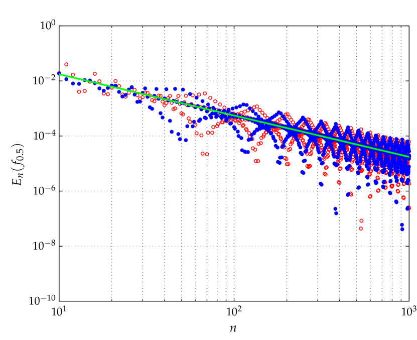
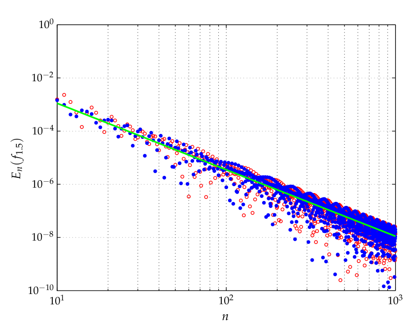
Figure 1. Numerical evidence that $n$-point Gauss quadrature has an $O(n^{-s-1})$ error rate for integrating the functions $f_{s}(x)=|x-0.3|^{s}$ (left: $s=0.5$, right: $s=1.5$) on the interval $(-1,1)$: $E_{n}^{G}(f_{s})$ (dots), $E_{n}^{C}(f_{s})$ (circles), $c_{s}n^{-s-1}$ (solid line).

Numerical experiments with $f_{s}(x)=|x-0.3|^{s}$, which is of class $X^{s}$ (see §2), and various $0<s<2$ (as in Fig. 1) has led us to the conjecture that Gauss quadrature enjoys the same $O(n^{-s-1})$ error rate as Clenshaw–Curtis also for $0<s<2$ in general. We remark that these experiments also show that the $O(n^{-s-1})$ error rate cannot be improved for any of the two quadrature rules.

Quadrature vs. best approximation

In his detailed study of the almost equal numerical performance of the quadrature rules of Gauss and Clenshaw–Curtis for functions of various regularity types, ? proved a suboptimal $O(n^{-s})$ bound for functions $f\in X^{s}$. In the Gauss case he based his rate estimate on the classical bound $|E_{n}^{G}(f)|\leqslant 4E_{2n+1}^{*}(f)$ (see, e.g., ?, p. 333) where $E_{n}^{*}(f)$ denotes the error of best approximation by polynomials of degree $n$; if $f\in X^{s}$ this allows the straightforward estimate (see, e.g., ?, Thm. 3.3)

$$E^{*}_{n}(f)\leqslant\sum_{m=n+1}^{\infty}|a_{m}|=O(n^{-s}).$$

In the case $f(x)=|x|$ (which is of class $X^{1}$) the estimate is sharp, since it is known by a theorem of Bernstein that (?, Eq. (1.18))

$$\lim_{n\to\infty}nE_{n}^{*}(|x|)=0.2801694990\ldots\,.$$

Hence, Clenshaw–Curtis and Gauss quadrature converge with a rate that is typically one power of $n$ better than the one of polynomial best approximation.

2. Functions of class $X^{s}$

It is well known (see, e.g., ?, §4.8.1) that the Chebyshev coefficients $a_{m}$ of $f(x)$ are given by the Fourier coefficients of $f(\cos\theta)$:

$$a_{m}=\frac{2}{\pi}\int_{-1}^{1}\frac{f(x)T_{m}(x)}{\sqrt{1-x^{2}}}\,dx=\frac{2}{\pi}\int_{0}^{\pi}f(\cos\theta)\cos m\theta\,d\theta.$$

Asymptotic analysis of Fourier integrals can now be used to determine the decay rate of the $a_{m}$: e.g., the function $f_{s}(x)=|x-\xi|^{s}$ with $-1<\xi<1$ and $s>0$ is of class $X^{s}$ since by the method of stationary phase (?, §§3.11–3.13)

$$a_{m}=-\frac{4}{\pi}T_{m}(\xi)(1-\xi)^{s/2}\Gamma(1+s)\sin(\pi s/2)m^{-s-1}+o(m^{-s-1})\qquad(m\to\infty).$$

Alternatively (but often less sharp), decay estimates of Fourier coefficients based on the smoothness properties of $f$ can be used; e.g., (?, Thms. II.4.12):

Let $f$ be defined on $[-1,1]$. If $f(\cos t)$ is $k-1$-times differentiable with a piecewise $k$-th derivative of bounded variation, then $f\in X^{k}$.

Since all derivatives of $\cos t$ exist and are bounded by the constant $1$, the smoothness properties of $f(\cos t)$ can conveniently be inferred from those of $f(x)$ (but not vice versa). In particular, if $f$ itself is $k-1$-times differentiable with a piecewise $k$-th derivative of bounded variation, we still get $f\in X^{k}$.

Remark

Denoting the total variation of that piecewise $k$-th derivative of $f$ by $V$, ? proved the explicit bound

$$|a_{m}|\leqslant\frac{2V}{\pi m^{\underline{k+1}}}\qquad(m\geqslant k+1);$$

using it, ? rendered the rate estimate (1) in the explicit form

$$|E_{n}(f)|\leqslant\frac{\pi V}{2n^{\underline{k+1}}}$$

if $n$ is sufficiently large (and, for Gauss quadrature, $k\geqslant 2$); an estimate that would asymptotically be, for $f(x)=|x|$, just a factor of $2$ off the true state of affairs.

3. Convergence rate of Clenshaw–Curtis quadrature

Clenshaw–Curtis quadrature on $[-1,1]$ is the interpolatory $n$-point quadrature rule that is derived from the nodes

$$x_{k}=\cos\left(\frac{k-1}{n-1}\pi\right)\qquad(k=1,\ldots,n).$$ (3)

Now, it is well known that from $T_{m}(x)=\cos(m\arccos x)$ one reads off aliasing due to undersampling, that is, with $m=2j(n-1)+2r$ and $-(n-2)\leqslant 2r\leqslant n-1$

$$T_{m}(x_{k})=T_{2|r|}(x_{k});$$

which implies, since Clenshaw–Curtis is exact for polynomials of degree $n-1$,

$$I^{C}_{n}(T_{m})=I^{C}_{n}(T_{2|r|})=I(T_{2|r|}).$$

Here, $I_{n}^{C}(f)$ denotes the quadrature formula as applied to $f$ and $I(f)$ the integral. Therefore, as $m\geqslant n\to\infty$, the quadrature error $E_{n}^{C}(T_{m})$ satisfies

$$E_{n}^{C}(T_{m})=I(T_{m})-I(T_{2|r|})=-\dfrac{2}{m^{2}-1}+\dfrac{2}{4r^{2}-1}=\dfrac{2}{4r^{2}-1}+O(n^{-2}).$$

With $f\in X^{s}$, that is, $a_{m}=O(m^{-s-1})$ for some $s>0$, we follow the ideas of ? in estimating

$$|E_{n}^{C}(f)|\leqslant\sum_{q=n}^{\infty}|a_{q}|\cdot|E_{n}^{C}(T_{q})|=O(S_{1})+O(S_{2}),$$

where

$$S_{1}=\sum_{j=1}^{\infty}\sum_{|2r|<n}\dfrac{1/|4r^{2}-1|}{(2j(n-1)+2r)^{s+1}},\qquad S_{2}=n^{-2}\sum_{q=n}^{\infty}\frac{1}{q^{s+1}}=O(n^{-s-2}).$$

Because of

$$\sum_{r=-\infty}^{\infty}\dfrac{1}{|4r^{2}-1|}=2,\qquad\sum_{j=1}^{\infty}\frac{1}{j^{s+1}}=\zeta(s+1),$$ (4)

we immediately see that $S_{1}=O(n^{-s-1})$; hence we obtain the rate estimate

$$E_{n}^{C}(f)=O(n^{-s-1})\qquad(s>0),$$ (5)

which proves the theorem of §1 in the Clenshaw–Curtis case.

4. Convergence rate of Gauss quadrature I

As substitute for (3) there are asymptotic formulas for the nodes $x_{k}$ of $n$-point Gauss quadrature (the zeros of the Legendre polynomial of degree $n$): a classical one of ? is, writing $\phi_{k}=(4k-1)\pi/(4n+2)$ for short,

$$x_{k}=\cos\left(\phi_{k}+\tfrac{1}{8}\cot(\phi_{k})n^{-2}+O(k^{-2}n^{-1})\right)\qquad(1\leqslant k\leqslant n/2).$$ (6)

Using this and an $O(n^{-1})$ bound on the weights, ? proved that the error in integrating the Chebyshev polynomials is

$$E_{n}^{G}(T_{m})=\begin{cases}(-1)^{j}\dfrac{2}{4r^{2}-1}+O(m^{2}/n^{3})+O(m\log n/n^{2})&\quad-n<r<n,\\[17.07164pt] (-1)^{j}\dfrac{\pi}{2}+O(m^{2}/n^{3})+O(m\log n/n^{2})&\quad r=\pm n,\end{cases}$$

if $2n\leqslant m=j(4n+2)+2r$ with $-n\leqslant r\leqslant n$ and $j\geqslant 0$. This way, aliasing holds asymptotically for $m=o(n^{3/2})$ only; for larger $m$, phase errors of order $O(1)$ will render the estimate useless. Still, because of $|T_{m}|\leqslant 1$ on $[-1,1]$ we get the uniform bound $|E_{n}^{G}(T_{m})|\leqslant 4$. We now estimate $E_{n}^{G}(f)=E_{n}^{\prime}+E_{n}^{\prime\prime}$ by splitting the Chebyshev expansion at an index of the order $O(n^{1+\epsilon})$ with some $0<\epsilon<1$ to be chosen later. Using the uniform bound of $E_{n}^{G}(T_{m})$ we thus get the tail estimate

$$E_{n}^{\prime\prime}=\sum_{q=n^{1+\epsilon}}^{\infty}|a_{2q}|\cdot|E_{n}^{G}(T_{2q})|=O\left(\sum_{q=n^{1+\epsilon}}^{\infty}\dfrac{1}{q^{s+1}}\right)=O(n^{1-s\epsilon}n^{-s-1}).$$

We are left with estimating the first $O(n^{1+\epsilon})$ terms of the Chebyshev expansion:

$$E_{n}^{\prime}=\sum_{q=n}^{n^{1+\epsilon}}|a_{2q}|\cdot|E_{n}^{G}(T_{2q})|=O(S_{1}^{\prime})+O(S_{2}^{\prime}),$$

where

$$S_{1}^{\prime} =\sum_{j=1}^{\infty}\sum_{|r|<n}\dfrac{1/|4r^{2}-1|}{(j(4n+2)+2r)^{s+1}}+\sum_{j=1}^{\infty}\sum_{r=\pm n}\dfrac{1}{(j(4n+2)+2r)^{s+1}}+\dfrac{1}{n^{s+1}},$$

$$S_{2}^{\prime} =\dfrac{1}{n^{3}}\sum_{q=n}^{n^{1+\epsilon}}q^{1-s}+\frac{\log n}{n^{2}}\sum_{q=n}^{n^{1+\epsilon}}q^{-s}.$$

From (4) we immediately see that $S_{1}^{\prime}=O(n^{-s-1})$. Likewise, we obtain

$$n^{s+1}S_{2}^{\prime}=\begin{cases}O(n^{(2-s)\epsilon})&\quad 0<s<2,\\[5.69054pt] O(\log n)&\quad s\geqslant 2.\end{cases}$$

Summarizing, the optimized choice $\epsilon=1/2$ results in the rate estimate

$$E_{n}^{G}(f)=\begin{cases}O(n^{-3s/2})&\quad 0<s<2,\\[5.69054pt] O(n^{-s-1}\log n)&\quad s\geqslant 2.\end{cases}$$ (7)

which proves the theorem of §1 in the Gauss case up to a factor $\log n$.

5. Convergence rate of Gauss quadrature II

? observed that we can get rid of the logarithmic factor in (7) by using a refined estimate of ?: upon replacing the bound in (8) by a later, sharper one also due to ?, namely

$$x_{k}=\cos\left(\phi_{k}+\tfrac{1}{2}\cot(\phi_{k})(2n+1)^{-2}+O(k^{-3}n^{-1})\right)\qquad(1\leqslant k\leqslant n/2),$$ (8)

and by using some improved, individual estimates of the weights, Petras proved, within the range $m=O(n^{2})$, that

$$|E_{n}^{G}(T_{m})|=\begin{cases}\dfrac{2+O(mr/n^{2})}{|4r^{2}-1|}+O(m^{4}/n^{6})+O(m^{2}\log(n)/n^{4})&\,|r|<n,\\[14.22636pt] \dfrac{\pi}{2}+O(m/n^{2})+O(m^{4}/n^{6})+O(m^{2}\log(n)/n^{4})&\,|r|=n,\end{cases}$$

where $2n\leqslant m=j(4n+2)+2r$ with $|r|\leqslant n$ and $0\leqslant j=O(n)$. Thus, we obtain

$$E_{n}^{\prime}=\sum_{q=n}^{n^{1+\epsilon}}|a_{2q}|\cdot|E_{n}^{G}(T_{2q})|=O(S_{1}^{\prime})+O(\tilde{S}_{1}^{\prime})+O(\tilde{S}_{2}^{\prime}),$$

where $S_{1}^{\prime}=O(n^{-s-1})$ is defined as in §4 and

$$\tilde{S}_{1}^{\prime} =\sum_{j=1}^{n^{\epsilon}}\sum_{|r|<n}\dfrac{jr/|4r^{2}-1|/n}{(j(4n+2)+2r)^{s+1}}+\sum_{j=1}^{n^{\epsilon}}\sum_{r=\pm n}\dfrac{j/n}{(j(4n+2)+2r)^{s+1}}+\dfrac{1}{n^{s+2}},$$

$$\tilde{S}_{2}^{\prime} =\dfrac{1}{n^{6}}\sum_{q=n}^{n^{1+\epsilon}}q^{3-s}+\dfrac{\log n}{n^{4}}\sum_{q=n}^{n^{1+\epsilon}}q^{1-s}.$$

By

$$\sum_{r=-n}^{n}\dfrac{r}{|4r^{2}-1|}=O(\log n),\qquad\dfrac{1}{n}\sum_{j=1}^{n^{\epsilon}}j^{-s}=O(n^{\epsilon-1}),$$

and, for $0<\epsilon<1$, $O(n^{\epsilon-1}\log n)=o(1)$ we get $\tilde{S}_{1}^{\prime}=O(n^{-s-1})$. Likewise

$$n^{s+1}\tilde{S}_{2}^{\prime}=\begin{cases}O(n^{(4-s)\epsilon}/n)&\quad 0<s<4,\\[2.84526pt] O(\log n/n)&\quad s\geqslant 4.\end{cases}$$

Summarizing, though the optimal choice $\epsilon=1/2$ just reproduces (7) for $0<s<2$, it results, this time, in the rate estimate

$$E_{n}^{G}(f)=O(n^{-s-1})\qquad(s\geqslant 2),$$ (9)

which finally proves the Gauss case of the theorem of §1.

6. Open problems

We leave the following open problems as challenges to the reader; their solution would require further, significant technical refinements of the methods used in this paper: to prove that, for $f\in X^{s}$,

• the convergence rate is $O(n^{-s-1})$ for Gauss quadrature if $0<s<2$;
  

• $|E_{n}^{G}(f)/E_{n}^{C}(f)|$ and its reciprocal stay uniformly bounded (cf. Fig. 1).

Acknowledgements

The authors thank Nick Trefethen for his continuing interest in this work and for his comments on some preliminary versions of the manuscript.

References

- [1]
- [2] [] Abramowitz, M. and Stegun, I. A.: 1965, Handbook of Mathematical Functions with Formulas, Graphs, and Mathematical Tables, Dover, New York.
- [3]
- [4] [] Bornemann, F.: 2010, On the numerical evaluation of Fredholm determinants, Math. Comp. 79(270), 871–915.
- [5]
- [6] [] Curtis, A. R. and Rabinowitz, P.: 1972, On the Gaussian integration of Chebyshev polynomials, Math. Comp. 26, 207–211.
- [7]
- [8] [] Davis, P. J. and Rabinowitz, P.: 1984, Methods of Numerical Integration, 2nd edn, Academic Press.
- [9]
- [10] [] Gatteschi, L.: 1956/1957, Limitazione degli errori nelle formule asintotiche per le funzioni speciali, Univ. e Politec. Torino. Rend. Sem. Mat. 16, 83–94.
- [11]
- [12] [] Gatteschi, L.: 1987, New inequalities for the zeros of Jacobi polynomials, SIAM J. Math. Anal. 18, 1549–1562.
- [13]
- [14] [] Gautschi, W. and Giordano, C.: 2008, Luigi Gatteschi’s work on asymptotics of special functions and their zeros, Numer. Algorithms 49, 11–31.
- [15]
- [16] [] Olver, F. W. J.: 1974, Asymptotics and Special Functions, Academic Press, New York.
- [17]
- [18] [] Petras, K.: 1995, Gaussian integration of Chebyshev polynomials and analytic functions, Numer. Algorithms 10(1-2), 187–202.
- [19]
- [20] [] Riess, R. D. and Johnson, L. W.: 1971/72, Error estimates for Clenshaw-Curtis quadrature, Numer. Math. 18, 345–353.
- [21]
- [22] [] Rivlin, T. J.: 1990, Chebyshev Polynomials, 2nd edn, John Wiley, New York.
- [23]
- [24] [] Trefethen, L. N.: 2008, Is Gauss quadrature better than Clenshaw-Curtis?, SIAM Rev. 50(1), 67–87.
- [25]
- [26] [] Trefethen, L. N.: 2012, Approximation Theory and Approximation Practice, SIAM, Philadelphia. (to appear).
- [27]
- [28] [] Varga, R. S. and Carpenter, A. J.: 1985, On the Bernstein conjecture in approximation theory, Constr. Approx. 1, 333–348.
- [29]
- [30] [] Xiang, S.: 2012, On the optimal convergence orders of Gauss, Clenshaw-Curtis, Féjer and Gauss-Chebyshev Quadrature, Technical report, Central South University, Changsha, Hunan, China.
- [31]
- [32] [] Zygmund, A.: 1968, Trigonometric Series I, 2nd edn, Cambridge University Press, London.
- [33]