Velocity renormalization and anomalous quasiparticle dispersion in extrinsic graphene

Abstract

Using many-body diagrammatic perturbation theory we consider carrier density- and substrate-dependent many-body renormalization of doped or gated graphene induced by Coulombic electron-electron interaction effects. We quantitatively calculate the many-body spectral function, the renormalized quasiparticle energy dispersion, and the renormalized graphene velocity using the leading-order self-energy in the dynamically screened Coulomb interaction within the ring diagram approximation. We predict experimentally detectable many-body signatures, which are enhanced as the carrier density and the substrate dielectric constant are reduced, finding an intriguing instability in the graphene excitation spectrum at low wave vectors where interaction completely destroys all particle-like features of the noninteracting linear dispersion. We also make experimentally relevant quantitative predictions about the carrier density and wave-vector dependence of graphene velocity renormalization induced by electron-electron interaction. We compare on-shell and off-shell self-energy approximations within the ring diagram approximation, finding a substantial quantitative difference between their predicted velocity renormalization corrections in spite of the generally weak-coupling nature of interaction in graphene.

I introduction

Graphene is a unique electronic material which consists simply of a single two-dimensional (2D) atomic membrane of carbon atoms in a honeycomb lattice. The seminal discovery novoselov2004 that graphene can be gated (i.e., “doped” with a finite free carrier density) to produce a variable carrier density ($n$) electron or hole 2D system simply by tuning an external gate voltage has given rise to a truly amazing level of intellectual activity with more that 10,000 graphene publications appearing in the scientific literature since 2005 covering many disparate fields including physics, chemistry, materials science, electrical engineering, and chemical engineering. From the fundamental perspective of quantum condensed matter physics graphene is an intriguing system dassarma2011 in many ways: it is a true 2D stable crystal with unique elastic and mechanical properties, and gated graphene is an exotic 2D gapless and chiral electron system with linear energy dispersion, i.e., the electron-hole bands in graphene have Dirac-Weyl massless linear dispersion instead of the usual parabolic energy dispersion one sees in most solid state materials. Graphene is thus both a semimetal and a gapless semiconductor, which can be easily doped by an external gate voltage to induce a variable carrier density $n$ (either electrons or holes) with a special charge neutrality point ($n\equiv 0$), often called the Dirac point, separating electron bands from the hole bands.

The purpose of the current work is to theoretically consider electron-electron interaction effects in gated graphene (i.e. $n\neq 0$), sometimes also called “extrinsic” graphene hwang2007a ; dassarma2007 to contrast with very special situation of “intrinsic” graphene ($n\equiv 0$) where the chemical potential is precisely located at the Dirac point. Since the Dirac point itself ($n=0$ precisely) is by definition a set of measure zero (particularly because of the gaplessness of graphene bands), most experiments can only probe extrinsic graphene (with $n\neq 0$) with any conclusion about the Dirac point being obtained indirectly through an extrapolation to zero density. The physics of graphene Dirac point is interesting in its own right as it is well-established dassarma2007 ; gonzalez1994 ; khvesh2001 that intrinsic graphene ($n=0$) is not a Fermi liquid. The presence of disorder-induced electron-hole puddlesdassarma2011 makes it difficult to study the physics of pristine Dirac point physics. Interaction physics at the Dirac point is outside the scope of the current work.

Since our interest is extrinsic gated graphene at $T=0$, we consider our starting noninteracting system to have the Fermi energy ($E_{F}$, or equivalently the chemical potential $\mu$) in the conduction band (with no loss of generality) given by $E_{F}=v_{0}(4\pi n/g)^{1/2}$, choosing $\hbar=1$ throughout, where $g=4$ is the graphene ground state degeneracy arising from spin (2) and valley (2) degeneracies. The Fermi wave vector $k_{F}=(\pi n)^{1/2}$ defines the 2D momentum upto which the conduction band with linear noninteracting band dispersion $E_{0}(k)=v_{0}k$, with $k=|{\bf k}|$ being the 2D wave vector, is filled. The linear band dispersion leads to a simple linear $E$ density of states, which then provides $k_{F}$, $E_{F}$, etc. quoted above dassarma2011 . Here $v_{0}\approx 10^{8}$ cm/s is the noninteracting graphene velocity obtained, for example, from band structure calculations dassarma2011 . Electron-electron interaction would affect the graphene noninteracting dispersion $E_{0}(k)=v_{0}k$, perhaps modifying the dispersion itself, i.e., changing the constant $v_{0}$, which is independent of both the carrier density and the substrate material supporting the graphene layer in the noninteracting single-particle approximation, to a renormalized wave vector-dependent nonlinear graphene velocity $v^{*}(k)$ which depends not only on $k$, but also on the carrier density $n$ and the substrate material (through the background dielectric constant $\kappa$).

The main goal of our work is to make precise (and experimentally verifiable) quantitative predictions about the interacting quasiparticle energy dispersion and the renormalized interacting velocity $v^{*}$ in gated extrinsic graphene which, in principle, may depend on wave vector, carrier density, and the substrate material. Quite surprisingly, this issue, in spite of its considerable importance, has not been studied in details in the existing theoretical literature as earlier work on the subject has concentrated mostly on interaction effects in intrinsic graphene dassarma2007 ; gonzalez1994 ; khvesh2001 ; elias2011 and the associated instabilities of the Dirac point or on the numerical calculations of the interacting spectral function in a narrow range of momentum and frequency polini2008 ; hwang2008 . In addition, we investigate the renormalized quasiparticle energy dispersion for different interaction strength (i.e. $r_{s}$) values to investigate instability at low energy regime (i.e., near the Dirac point). It is expected that the quasiparticle feature may be modified due to the many body effects (plasmonic feature) as seen in the ARPESarpes ; arpes1 ; arpes2 . However, unexpectedly we find that the quasiparticle features disappear as the interaction strength increases. In earlier workarpes some of the features presented here are discussed for small $r_{s}$ values ($r_{s}<0.5$). However, the instability due to many body effect is significantly enhanced for large $r_{s}$ and for low densities, which is not discussed elsewhere. This is a very interesting prediction and can be observed in samples with high $r_{s}$ value (for example, suspended graphene). In fact, we find that a careful experimental study of even the standard graphene on substrates should be able to discern our predicted signature of a dispersion instability in the spectral function.

We emphasize that there have been several theoretical investigations of interaction effects in graphenedassarma2011 ; hwang2007a ; dassarma2007 ; gonzalez1994 ; khvesh2001 ; elias2011 ; polini2008 ; hwang2008 ; arpes ; arpes2 including some by us hwang2007a ; dassarma2007 ; hwang2008 as well as a few careful experimental studies elias2011 ; arpes ; arpes1 ; arpes2 comparing with the theoretical predictions. Our work is based on existing dassarma2011 ; hwang2007a ; dassarma2007 ; polini2008 ; hwang2008 and well-established theoretical techniques (namely, Feynman-Dyson diagrammatic perturbation theory using the dynamically screened Coulomb interaction as the effective coupling constant – a technique that goes back to the 1960s and has been used extensively and successfully to calculate many-body interaction effects on single-particle properties in metals, doped semiconductors, and 2D electron systems as well as in band structure calculations under the name of ’$GW$ approximation’). In spite of the existing theoretical literature dealing with the calculation of electron-electron interaction-induced many-body renormalization effects in doped graphene, the results presented in the current work are completely new and are directly relevant to experimental measurements. Although based on the standard $GW$-type theoretical approximation our numerical results for the coupling constant dependent graphene Fermi velocity as well as the wave vector dependent graphene velocity are unavailable in the literature. These quantities can be measured directly by STM/STS or ARPES measurements to be compared with our theoretical results. Similarly, our results for the anomalous quasiparticle dispersion and the associated collapse of the quasiparticle picture for graphene at low carrier densities are new although the graphene spectral function itself has earlier been calculated in the literature polini2008 ; hwang2008 ; arpes ; arpes1 ; arpes2 . Finally, our comparison between on-shell and off-shell self-energy approximations for graphene many-body renormalization has not earlier been investigated in the graphene literature where all earlier work specifically considered the off-shell solution of the Dyson equation.

The rest of the paper is organized as follows. In Sec. II we discuss the general theory of the self-energy of graphene. In Sec. III we present our calculated renormalized Fermi velocities within on-shell and off-shell approximations. In Sec. IV we show the detail results of the quasiparticle spectral function and the instability of the graphene dispersion, and finally we conclude in Sec. V.

Figure 1: Self-energy contribution [(a)-(d) plus all higher-order ring diagrams] included in our theory with the wiggly and the non-wiggly lines representing the bare interaction ($V$) and Green’s function ($G_{0}$) respectively. Figures (e) and (f) represent two second-order contributions ignored in the theory, which may approximately cancel each other leading to the on-shell approximation being quantitatively “better” than the off-shell Dyson’s solution.

II self-energy

The central theoretical quantity we calculate is the graphene dynamical self-energy function $\Sigma(k,E)$, which, in general, depends both on momentum (wave vector) and energy (frequency) independently. An exact theoretical evaluation of the self-energy for electrons interacting via the long-range Coulomb interaction ($V$) is, of course, impossible for arbitrary carrier density and interaction strength, but an excellent approximation scheme, which goes by the various nomenclatures such as the $GW$-approximation or the dynamical RPA, is well-established for parabolic metallic 2D and 3D electron systems. This approximation involves calculating the self-energy in an infinite order diagrammatic perturbation theory including all diagrams containing (to all orders) the bare Coulomb interaction, the bare electron Green’s function, and the bare polarizability (i.e., the bubble or the ring diagrams formed by the closed loop of an electron and a hole propagator). Equivalently, this infinite series of ring diagrams (we show in Fig. 1 the self-energy diagrams of the theory) corresponds to the leading-order perturbation expansion in the dynamically screened Coulomb interaction ($W$) where the screening is done by the electronic dynamical dielectric function ($\epsilon$) obtained in the random phase approximation (RPA) involving the infinite series of ring diagrams hwang2007 .

The validity of considering RPA type diagrams is based on the infrared divergence of the ring diagrams. All non-RPA diagrams are negligible compared with the same order RPA diagram. The divergence can be controlled by the RPA re-summation as shown in Fig. 1. The justification for why non-RPA diagrams in graphene can be neglected is discussed in Ref. dassarma_un, . We also emphasize that there is no known controlled technique for systematically calculating quasiparticle properties in interacting electron systems other than the $GW$ approximation based on RPA. Within the leading-order dynamical RPA the self-energy $\Sigma(k,E)$ of graphene is given bymahan ; hedin

$$\Sigma_{s}(k,i\omega_{n})=-\frac{1}{\beta}\sum_{s^{\prime}}\sum_{{q},i\nu_{n}}G_{0,s^{\prime}}(k+q,i\omega_{n}+i\nu_{n})$$

$$\times W(q,i\nu_{n})F_{ss^{\prime}}({k},{k}+{q}),$$ (1)

where $\beta=1/k_{B}T$ is the inverse temperature, $W$ is the screened Coulomb interaction, $G_{0}(k,i\omega_{n})=[i\omega_{n}-E_{0}(k)+\mu]^{-1}$ is the bare Green’s function (where $\omega_{n},\nu_{n}$, and $\mu$ are Matsubara fermion, boson frequencies and chemical potential, respectively)mahan . Due to the chiral property of graphene the self-energy in Eq. (1) has an additional term (i.e., $F_{ss^{\prime}}$) which does not exist in the non-chiral systems. The $F_{ss^{\prime}}$ arises from the overlap of $\mathinner{|}\!s{k}\rangle$ and $\mathinner{|}\!s^{\prime}{k}^{\prime}\rangle$ and is given by $F_{ss^{\prime}}({k},{k}^{\prime})=\frac{1}{2}(1+ss^{\prime}\cos\theta_{{kk}^{\prime}})$, where $s,s^{\prime}=\pm 1$ are band indices of graphene and $\theta_{{kk^{\prime}}}$ is the angle between ${k}$, ${k}^{\prime}$. The screened Coulomb interaction $W(q,i\nu_{n})=V(q)/\epsilon(q,i\nu_{n})$, where $V(q)=2\pi e^{2}/\kappa q$ is the bare Coulomb potential ($\kappa=$background dielectric constant), and $\epsilon(q,i\nu_{n})$ is the 2D dynamical dielectric function. In the RPA $\varepsilon(q,i\nu_{n})=1-V(q)\Pi_{0}(q,i\nu_{n})$, where $\Pi_{0}=G_{o}G_{0}$ is the noninteracting polarizabilityhwang2007 . The expression for $\Sigma$, $W$, $\Pi_{0}$ involve multidimensional complex integrals over internal momentum and energy.

Since there has been substantial earlier work in the literature on the theory of the electron self-energy within the dynamical RPA $GW$ approximation in systems as different as 3D electron gas hedin , 2D electron gas jalabert , 1D electron gas hu1993 , monolayer graphene polini2008 ; hwang2008 ; leblanc ; dassarma_un , and bilayer graphene sensarma2011 , we refrain from giving more theoretical details on our calculations, concentrating instead on the results and their experimental implications for observable many-body effects in gated graphene.

We note that ($i$) the calculation of the self-energy $\Sigma$ leads immediately to the interacting Green’s function $G$, [i.e. $G^{-1}=G_{0}^{-1}-\Sigma$] which contains all information about the single-particle properties of graphene, and that (ii) once the bare polarizability $\Pi_{0}$, which was earlier obtained hwang2007 , is known, the calculation of self-energy [Eq. 1] would lead to $G$ since $G_{0}$ and $V$ are known by definition. We note that we are utilizing the leading-order “$G_{0}W$” rather than the self-consistent “$GW$” approximation in our theory. We believe the $G_{0}W$ approximation to be more meaningful from a diagrammatic perturbative sense since it is a true leading-order expansion in the effective RPA screened dynamical interaction $W$ whereas the iterative $GW$ approximation mixes in unwanted higher-order terms in $W$ which are inconsistent with the leading-order expansion in $W$.

We emphasize that the graphene self-energy calculation is highly nontrivial and extremely subtle because one must include both intraband and interband contributions in the theory. Remembering that the noninteracting Green’s function $G_{0}=[E-E_{0}(k)]^{-1}$ has its poles at the noninteracting energy $E_{0}=v_{0}k$, we get the following equation for the poles of the interacting Green’s function $E=E_{0}+\Sigma(k,E)$, which defines a general integral equation (Dyson equation) for the interacting graphene dispersion:

$$E(k)=E_{0}(k)+{\rm Re}\Sigma[k,E(k)].$$ (2)

We note that $\Sigma(k,E)$ is, in general, complex and the quasiparticle energy (damping) for the interacting system is given by the real (imaginary) part of the self-energy. We solve the integral equation defined by Eq. (2) numerically iteratively to obtain the interacting quasiparticle dispersion $E(k)=v_{1}^{*}(k)k$, and refer to this iterative solution as the “off-shell” approximation which alludes to the full solution of the Dyson equation. An alternative approximation for the self-energy, the so-called on-shell approximation, goes back to the early days of diagrammatic many-body theory dubois1959 , and has, in particular, been emphasized by Rice rice1965 . In the on-shell approximation, one simply takes the first iterative solution of Eq. (2) to get

$$E(k)=E_{0}(k)+{\rm Re}\Sigma[k,E_{0}(k)],$$ (3)

which does not involve solving the Dyson integral equation. This would define an on-shell graphene velocity given by $E(k)=v_{2}^{*}(k)k$. Note that the imaginary part of on-shell self energy near Fermi surface behaves as Im[$\Sigma[k,E_{0}(k)]\propto[E_{0}(k)-\mu]^{2}\ln[E_{0}(k)-\mu]$, where $\mu=E_{0}(k_{F})$. dassarma2007 Thus the on-shell imaginary part of the self-energy certainly vanishes as $k\rightarrow k_{F}$. In fact, the inelastic scattering rate, an extensively used physical quantity of much experimental interest, is precisely the on-shell approximation to the Im[$\Sigma(k,E)]$. We will compare the on-shell and the off-shell graphene self-energy solution within our dynamical RPA scheme because the issue of which of these two is a better approximation to the Coulomb self-energy problem has been much discussed in the literature over the last 50 years dubois1959 ; rice1965 ; ting1975 ; vinter1975 ; zhang2005 . These past discussions of course focused only on regular nonchiral parabolic electron systems with only intraband contributions and our current work is on chiral, linearly dispersing, gapless graphene carriers where both intra- and inter-band contributions to the self-energy must be included in the theory (as we do in our current work). We note that there is no deep principle that could make the ”correct” theoretical choice between the on-shell and the off-shell approximation within the $G_{0}W$ self-energy scheme since both schemes obey the Ward identity and the Dyson equation up to the order in the interaction the theory is meant to be valid. (i.e., leading order in the dynamically screened interaction $W$). The only effective choice between these approximations is an operational one based on the detailed quantitative comparison with the experimental data as has already been discussed in the past rice1965 ; ting1975 ; vinter1975 ; zhang2005 .

It may be worthwhile for us to make some remarks on the on-shell versus off-shell many-body self-energy approximation in the context of graphene physics, and why this may be a question of substantial importance. This issue arises because the dynamical Coulomb self-energy can only be calculated approximately in the leading-order GW-RPA approximation. If an exact self-energy function $\Sigma(k,E)$ is available, then obviously the full Dyson equation solution would be necessary to obtain the quasiparticle energy dispersion $E(k)$, making the off-shell velocity the only meaningful quantity. It has, however, been pointed out dubois1959 ; rice1965 ; ting1975 ; vinter1975 ; zhang2005 that the leading-order screened interaction expansion (i.e., the ring diagram approximation) for the calculated RPA self-energy necessitates using the leading-order iterative solution of $\Sigma(k,E)$, i.e., using the on-shell approximation $\Sigma(k,E_{0}(k))$, instead of the full solution of the integral Dyson equation so as not to mix various orders of approximation in the theory. In particular, it has been arguedrice1965 that the on-shell approximation of the self-energy is, in fact, quantitatively better than the off-shell approximation within the GW-RPA scheme of the Coulomb self-energy evaluation for metallic electrons. The subject has been controversial ting1975 ; zhang2005 ; vinter1975 with no definite consensus in the literature in spite of the almost 50-year history of the topic. Our careful quantitative comparison of on-shell and off-shell approximations, when compared with the available experimental data in graphene should lead to a resolution of this old and important theoretical controversy. Our results tend to indicate that the off-shell approximation works better for graphene as described below.

We emphasize, so that there is no misunderstanding of this point, that if the self-energy is evaluated exactly then one must always solve the Dyson equation, and as such the off-shell theory defined by Eq. (2) is the only option for the quasiparticle dispersion in any exact theory. The question arises, however, whether solving the Dyson equation is always preferable for obtaining the quasiparticle energy dispersion $E(k)$ even when the self-energy has been calculated in an approximate theory. In particular, if the self-energy is calculated in the leading-order expansion in the dynamically screened Coulomb interaction, as it is in the current RPA-ring diagram $GW$ theory and in all the existing theories in the literature, then it is unclear which approximation, on-shell or off-shell, is a better quantitative approximation.

Iterating Eq. (2) formally order by order, i.e., solving the implicit integral equation for the off-shell self-energy defined by Eq. (2) through the standard iterative technique, we get

$$E_{1}(k) = E_{0}(k)+\Sigma(k,E_{0}(k))$$

$$E_{2}(k) = E_{0}(k)+\Sigma(k,E_{0}(k)+\Sigma(k,E_{0}(k)))$$

$$E_{3}(k) = E_{0}(k)+\Sigma(k,E_{0}(k)+\Sigma(k,E_{0}(k)+\Sigma(k,E_{0}(k))))$$

$$E_{4}(k) = ...$$

We note that the leading-order iterative solution above is the same as the on-shell approximation defined in Eq. (3). We now note that the $GW$ approximation used in the current (and many other) work involves (see Fig. 1) calculating the self-energy formally as a leading-order expression in the screened Coulomb interaction $\Sigma\sim W$, and as such all iterations of the self-energy beyond the on-shell approximation must necessarily involve terms which are formally higher order in $W$, which would be inconsistent with the leading order $GW$ calculation. This is in fact the argument behind the claim that the on-shell approximation may be a better approximation than the off-shell one within the leading-order $GW$ theory. Within this leading-order theory there is no obvious way to claim that the full solution of the Dyson equation (i.e. the off-shell approximation) is necessary better than the leading-order solution of the Dyson equation (i.e. the on-shell approximation) since the former necessarily includes only an uncontrolled subset of higher-order terms in the screened interaction whereas the latter is manifestly leading-order in the screened interaction everywhere. We therefore provide results for both on-shell and off-shell approximations for future comparison with experiments.

III Renormalized Fermi velocity

For a given self-energy we can calculate the Fermi velocity by differentiating the self-energy with respect to the wave vector at $k=k_{F}$, that is, $v^{*}(k)=dE(k)/dk|_{k=k_{F}}$. The renormalized Fermi velocities $v_{F}^{*}$ corresponding to the appropriate self-energies of Eqs. (2) and (3), respectively, are given by

$$\frac{v_{1}^{*}(k)}{v_{0}}=\frac{1+\frac{1}{v_{0}}\frac{\partial}{\partial k}{\rm Re}\Sigma(k,\omega)|_{\omega=E(k)}}{1-\frac{\partial}{\partial\omega}{\rm Re}\Sigma(k,\omega)|_{\omega=E(k)}},$$ (4)

$$\frac{v_{2}^{*}(k)}{v_{0}}=1+\frac{1}{v_{0}}\frac{d}{dk}{\rm Re}\Sigma[k,E_{0}(k)],$$ (5)

and $v_{F_{1}}^{*}=v_{1}^{*}(k=k_{F})$, $v_{F_{2}}^{*}=v_{2}^{*}(k=k_{F})$. In our calculation of the on-shell velocity at the Fermi surface ( $k=k_{F}$ and $E_{0}(k)=E_{F}$), we take the limit of both $k$ and $\omega=E_{0}(k)$ going to the Fermi surface simultaneously. Along this path the imaginary part of the self energy becomes identically zero at the Fermi surface. However, taking $k$ and $E_{0}(k)$ to the Fermi surface independently gives rise to the different results and would be incorrect. We note that, while $v_{F}^{*}$ (both for on-shell and off-shell approximations) depends on the coupling constant (i.e., the background dielectric constant $\kappa$) and the carrier density ($n$), the general renormalizied graphene velocity $v^{*}(k)$ depends also on the momentum $k$, implying that the interacting quasiparticle graphene energy dispersion $E(k)$ is no longer simply linear in $k$ (as the noninteracting energy $E_{0}=v_{0}k$ is) even for a given substrate and fixed density. Thus, we have $v^{*}(k)\equiv v^{*}(k;n,\kappa)$; $v_{F}^{*}\equiv v_{F}^{*}(n,\kappa)$, and depending on the approximation scheme (off-shell or on-shell) we have two distinct renormalized velocities $v_{1,2}^{*}$. A main goal of our work is to obtain the ($k,n;\kappa$) dependence of the graphene quasiparticle velocity.

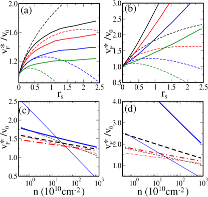
Figure 2: Calculated renormalized Fermi velocity (a) within the off-shell approximation, $v^{*}_{F_{1}}/v_{0}$, and (b) within the on-shell approximation, $v^{*}_{F_{2}}/v_{0}$, as a function of $r_{s}$ for several different densities, $n=10^{10}$, $10^{11}$, $10^{12}$, and $10^{13}$ cm^-2 (from top to bottom). The dashed lines represent the asymptotic results for small $r_{s}$ given by Eq. (6). In (c) and (d) the renormalized Fermi velocityies (thick lines) within the off-shell approximation and within the on-shell approximation are shown, respectively, as a function of carrier density for several different $r_{s}$, $r_{s}=0.5$ (dod-dashed lines), $r_{s}=0.8$ (dashed lines), and $r_{s}=2.2$ (solid lines). The thin lines represent the asymptotic results for small $r_{s}$ given by Eq. (6).

Before presenting our full numerical results (Figs. 2 and 3) which is one of our two main results in this work, we give the leading-order analytic result for the Fermi velocity $v_{F}^{*}\equiv v^{*}(k=k_{F})$ for gated graphene

$$\frac{v_{F}^{*}}{v_{0}}=1-\frac{r_{s}}{\pi}\left[\frac{5}{3}+\ln r_{s}\right]+\frac{r_{s}}{4}\ln\frac{k_{c}}{k_{F}},$$ (6)

where $r_{s}\equiv e^{2}/(v_{0}\kappa)$ is the so-called (background dielectric constant dependent) graphene fine-structure constant which defines the dimensionless electron-electron interaction strength or the Coulomb coupling constant for the problem and $k_{c}\sim 1/a$ (where $a$ is the graphene lattice size) is the ultraviolet cut-off for the problem. Throughout this paper $k_{c}=1/(2.46$Å) is used. Here $\kappa=(\kappa_{s}+1)/2$ where $\kappa_{s}$ is the lattice dielectric constant of the substrate material. The analytic formula given in Eq. (6) has earlier been derived in the literature dassarma2007 , and we provide it here for the sake of completeness and comparison.

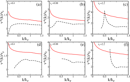
Figure 3: The calculated $v^{*}(k)$ as a function of $k/k_{F}$ are shown for (a) $r_{s}=0.4$, (b) $r_{s}=0.88$, and $r_{s}=2.2$ and a fixed carrier density $n=10^{12}$ cm^-2. The black dashed (red solid) line indicates the renormalized Fermi velocity within off-shell (on-shell) approximation. In (c) the velocity within off-shell is not defined for $k/k_{F}\lesssim 0.3$ (i.e., there is no solution in Dyson’s equation correpsonding to the quasiparticle.) In (d), (e), and (f) we show $v^{*}(k)$ for carrier density $n=10^{10}$ cm^-2 and $r_{s}=0.4$, $r_{s}=0.88$, and $r_{s}=2.2$, respectively. Since there are no solutions in Dyson’s equation correponding to the quasiparticle the renormalized off-shell velocity at small $k$ is not shown in (d), (e), and (f).

It is important to emphasize that Eq. (6) applies to both on-shell and off-shell approximations as they have exactly the same leading-order expansions in $r_{s}$, and Eq. (6) provides an exact expression in the $r_{s}\rightarrow 0$ limit since the ring diagrams are the most divergent diagrams in this leading-order (in $r_{s}$) limit. A curious feature of Eq. (6), which is completely unique to graphene with its linear massless and gapless energy dispersion, is that the velocity renormalization depends on two distinct dimensionless coupling parameters, $r_{s}$ [$\propto(v_{0}\kappa)^{-1}$] and $k_{c}/k_{F}$ [$\propto(\sqrt{n}a)^{-1}$] arising respectively from the Coulomb interaction strength ($r_{s}$) and the ultraviolet lattice cut-off ($k_{c}/k_{F}$). In ordinary parabolic electron systems, the Coulomb coupling strength $r_{s}$ itself depends on the carrier density (e.g., in 2D parabolic electron systems with a mass $m$, $r_{s}\sim m/\sqrt{n}$), and no ultraviolet cut-off is necessary. Thus, graphene is a very special and interesting Coulomb system with the interaction strength $r_{s}$ itself being density independent, but renormalization effects being logarithmically density dependent through the ultraviolet divergence. Such logarithmic dependence on the ultraviolet cut-off, while being common in relativistic field theories, is rare in solid state physics where the infrared Coulomb divergence is typically the main problem. We also mention that the second term (the square bracket) in Eq. (6) and the last term [containing $\ln(k_{c}/k_{F})$] arise respectively from intraband and interband transitions. Depending on the carrier density and the background dielectric constant, one or the other contribution could dominate, but in general both must be kept in the theory for extrinsic graphene. We note that the ultraviolet logarithmically divergent term in Eq. 6 goes as $\ln(n/n_{c})$ where $n_{c}$ is the cut-off density defining $k_{c}$, and as such the ultraviolet renormalization of the graphene coupling constant can be directly studied by tuning the carrier density $n$ with its effect being larger for larger $r_{s}$.

In Fig. 2 we show our full numerical calculations for the renormalized graphene velocity in the off-shell [Fig. 2(a)] and on-shell [Fig. 2(b)] approximations as a function of $r_{s}$ for different carrier densities ($n$) comparing the results with the analytic formula given by Eq. (6). In Figs. 2((c) and (d) the renormalized velocities as a function of density $n$ for different $r_{s}$ values are shown. Several features stand out in Fig. 2: ($i$) the velocity renormalization is a strong function of both $r_{s}$ and $n$ in both approximation schemes; ($ii$) the renormalization is substantially stronger in the on-shell than in the off-shell approximation; ($iii$) the leading-order analytic formula [Eq. (6)] applies only for $r_{s}\lesssim 0.4-0.8$ depending on the density and the approximation scheme.

In Fig. 3 we show our numerically calculated $v^{*}(k)$ for three different $r_{s}$ values as a function of momentum for the fixed carrier density $n=10^{12}$ cm^-2 for both approximation schemes. There are several interesting features of Fig. 3: ($i$) both approximations imply weak nonlinearity in the renormalized graphene quasiparticle dispersion except for $k<0.4k_{F}$; ($ii$) the many-body renormalization is substantially stronger for the on-shell approximation; ($iii$) at low momentum, $k\lesssim 0.5k_{F}$, the off-shell (on-shell) renormalization indicates nonlinear negative (positive) velocity corrections in graphene; ($iv$) as $r_{s}$ increases or at low densities the renormalized off-shell velocity is strongly nonlinear; ($v$) for large $r_{s}$ values or at low densities the renormalized off-shell velocity is not defined at small $k$, that is, there is no solution in Dyson’s equation [see Eq. (2)] corresponding to the quasiparticle energy. Thus the quasiparticle feature at low momentum disappears at high $r_{s}$ values or at low densities. We emphasize that some aspects of this physics were already apparent in Ref. [arpes, ], but the effect should be much more pronounced at higher (lower) $r_{s}$ ($n$) values.

One feature of Figs. 2 and 3 requires particular emphasis since it is quite non-obvious: On-shell and off-shell approximations start deviating from each other substantially already in the rather weak-coupling situation of $r_{s}\gtrsim 0.5$. Thus, it is clearly important to know by comparing with experiments which one is the better approximation.

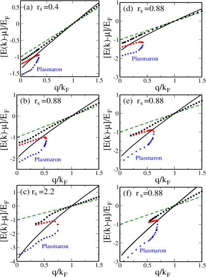
Figure 4: The renormalized quasiparticle energy dispersions as a function of wave vector for the electron density $n=10^{12}$ cm^-2 and for various $r_{s}$, (a) $r_{s}=0.4$, (b) $r_{s}=0.88$, and (c) $r_{s}=2.2$. In (d)(e)(f) the renormalized quasiparticle energy dispersions are shown as a function of wave vector for a fixed $r_{s}=0.88$ and for different electron densities (d) $n=10^{13}$ cm^-2, (e) $n=10^{11}$ cm^-2, and (f) $n=10^{10}$ cm^-2. Green dashed (black solid) lines represent the non-interacting (on-shell) energy dispersion, and symbols are the solutions of the Dyson’s integral equation. The dots (triangles) represent the dispersion of off-shell quasiparticle mode (plasmaron modes). The squares indicate the dispersion of the overdamped mode, which has insignificant spectral weight.

IV quasiparticle dispersion and spectral function

Although Figs. 2 and 3 present one of our main quantitative theoretical results showing the density, coupling constant, and momentum dependence of the renormalized graphene quasiparticle velocity, we now provide some calculated results for the many-body quasiparticle dispersion and spectral function since the quasiparticle velocity is derived from the quasiparticle energy dispersion [c.f. $E(k)=v^{*}(k)k$] which is contained in the interacting spectral function of the system. Even though we have used the well known many body diagrammatic perturbation theory ($G_{0}W$ approximation) we find very interesting and experimentally relevant results in the graphene energy dispersion which have not been discussed in the existing literature. These results are quite unanticipated.

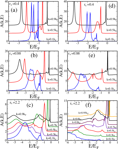
Figure 5: Calculated quasiparticle spectral function $A(k,E)$ as a function of energy for different wave vectors and three different $r_{s}$ values. The lines for different wave vectors are shifted upward for clarity. In (a), (b), and (c) the density $n=10^{12}cm^{-2}$ is used, and the density $10^{10}cm^{-2}$ is used in (d), (e), and (f).

In Fig. 4, we show our calculated quasiparticle energy dispersion for different densities and $r_{s}$ values. In (a), (b), and (c) results for a fixed density $n=10^{12}$ cm^-2 and for different $r_{s}$ values ($r_{s}=0.4$, 0.88, and 2.2 respectively) are shown, and in (d), (e), and (f) results for a fixed $r_{s}=0.88$ and for different densities ($n=10^{13}$, $n=10^{11}$ and $n=10^{10}$ cm^-2, respectively) are shown in both on-shell and off-shell approximations comparing them with the noninteracting energy dispersion $E_{0}(k)=v_{0}k$. The Fermi velocity in each case is given by the $k=k_{F}$ point. We note that $r_{s}=0.4$, 0.88, 2.2 correspond to graphene on SiC (or BN), SiO₂, vacuum, respectively. The important thing to note is that the on-shell approximation indicates very strong quasiparticle dispersion renormalization, particularly for suspended graphene ($r_{s}=2.2$), which may be unphysical, thus perhaps ruling out the validity of the on-shell approximation. Consistent with the results presented in Fig. 2, the off-shell approximation predicts rather small many-body dispersion (and velocity) renormalization, but it does make a very dramatic prediction about the complete failure of the quasiparticle picture for small momentum in suspended graphene ($r_{s}=2.2$). In particular, the off-shell quasiparticle mode for $r_{s}=2.2$ (and $n=10^{12}$ cm^-2) completely disappears for $k<0.4k_{F}$ (we have checked the same to be true for other carrier densities also), leaving only a weak plasmaron mode which shows up for all $r_{s}$ values at low wave vectors. Thus a clear prediction of our theory is that the quasiparticle dispersion in suspended graphene ($r_{s}=2.2$) will look dramatically different for $k\lesssim 0.5k_{F}$ with the complete disappearance of any particle-like feature in the graphene dispersion. As shown in Fig. 4(f) we find that the similar feature (i.e. the complete disappearance of a particle-like feature) develops as the density decreases. For $r_{s}=0.88$ and high enough densities [$n>10^{11}cm^{-2}$, see Fig. 4(b) and (d)] the quasiparticle-like dispersion is well defined even at $q=0$, but for $n\lesssim 10^{11}cm^{-2}$ the quasiparticle feature starts to disappear near $q=0$. Thus, there are two distinct ways of approaching ’strong-coupling’ in graphene either by going to smaller $k_{F}$ (i.e. lower density) keeping $r_{s}$ fixed or by keeping $k_{F}$ (or density) fixed and increasing $r_{s}$. However, these two strong-coupling approaches give non-equivalent results as shown in Fig. 4. Note that in ordinary electron 2D gas only changing $r_{s}$ is allowed to approach the strong coupling limit whereas in graphene one has one more adjustable parameter to approach the strong coupling limit, i.e., by changing $r_{s}$ through background dielectric constant of substrate and by changing $k_{F}$ through the back gate voltage. Since some aspects of this interesting physics were already observed in Ref. [arpes, ] we believe that experiments at higher (lower) $r_{s}$ ($n$) values should lead to a striking confirmation of our theoretical predictions.

This prediction can be directly tested in ARPES arpes ; arpes1 ; arpes2 and STS luican2011 ; sts ; sts2 measurements. Earlier theoretical workpolini2008 ; hwang2008 on the graphene spectral function completely missed this bizarre collapse of the quasiparticle picture for suspended graphene since they polini2008 ; hwang2008 focused on graphene on substrates. We note that $r_{s}=2.2$ is a relatively weak-coupling regime compared with 3D metals ($r_{s}\sim 3-6$) and 2D semiconductors ($r_{s}\sim 5-30$) where no such dispersion instability in the interacting spectral function has ever been predicted.

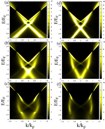
Figure 6: Density plot of the quasiparticle spectral function $A(k,E)$ as a function of energy $E/E_{F}$ and wave vectors $k/k_{F}$ for three different $r_{s}$ values, (a) and (d) $r_{s}=0.4$, (b) and (e) $r_{s}=0.88$, (c) and (f) $r_{s}=2.2$. In (a), (b), and (c) the density $n=10^{12}cm^{-2}$ is used, and the density $10^{10}cm^{-2}$ is used in (d), (e), and (f).

To further emphasize the low wave vector interaction-driven instability in the graphene quasiparticle spectrum discussed above, we show in Fig. 5 our calculated interacting graphene spectral function given by $A(k,E)\equiv-2{\rm Im}G(k,E)$, which directly provides the spectral strength of $E(k)$ features in the graphene spectrum with the noninteracting result being precisely $A_{0}(k,E)=2\pi\delta[E-E_{0}(k)]$. The calculated spectral function in Fig. 5 clearly shows that for $r_{s}=2.2$, the single particle-like feature disappears completely from the graphene spectral function for $k<0.5k_{F}$ ($0.7k_{F}$) for $n=10^{12}$ ($10^{10}$) cm^-2, and the spectral weight basically gets distributed broadly over the incoherent background. For $r_{s}=0.4$ (graphene on SiC or BN), however, some sharp spectral features persist down to low wave vectors, whereas graphene on SiO₂ ($r_{s}=0.88$) is intermediate in nature with sharp particle-like spectral features being present in the spectrum at low wave vectors and at high density, but disappearing at low density. Our theory, which has direct observable consequences for graphene experiments, thus predicts that the whole linear dispersing noninteracting energy band picture in graphene should completely collapse in suspended graphene for $k\lesssim 0.5k_{F}$ in the $10^{10}-10^{12}$ cm^-2 density range where all the spectral weight should disappear into a broad incoherent background due to electron-electron interaction. We emphasize that earlier graphene spectral function calculations polini2008 ; hwang2008 completely missed this dramatic behavior arising from the linear chiral nature of graphene.

To clearly see the disappearance (instability) of the graphene energy dispersion at small wave vectors (near Dirac point), in Fig. 6 we show the calculated spectral function, $A(k,E)$, as a color plot in $k/k_{F}$ and $E/E_{F}$ space for two different densities (a),(b),(c) $n=10^{12}cm^{−2}$ and (d),(e),(f) $n=10^{10}cm^{−2}$, respectively. In this figure the narrow bright area indicates the highest spectral weight. For $r_{s}=0.4$ [(a) and (d)] the single particle-like linear dispersion has the most spectral weight and well defined plasmaron features appear below the single particle-like peak. However for $r_{s}=2.2$ [(c) and (f)] there are no well defined peaks at small wave vectors and the spectral weight is distributed broadly over the incoherent background. The broadening of spectral weight at small wave vectors is more pronounced at low density (f). The disappearance (instability) develops gradually as the wave vector decreases, and the anomalous dispersion is stronger for lower density and higher $r_{s}$. We suggest that spectral function measurements via ARPES or STS be carried out on suspended graphene to directly observe our predicted instability.

V conclusion

To conclude, we have provided the detailed quantitative results for nonlinear interacting graphene dispersion as a function of density, coupling constant, and momentum, predicting in the process a spectacular collapse of the quasiparticle picture in suspended graphene for $k\lesssim 0.5k_{F}$, which can be directly tested in experiments. Our results indicate that many-body renormalization of graphene velocity is possible up to a factor of two as a function of either carrier density or wave vector if a large range of density and wave vector can be explored in future experiments. Our work is a generalization of earlier works polini2008 ; hwang2008 ; arpes in the literature to large $r_{s}$ values and lower carrier densities where the anomalous dispersion properties of graphene should lead to a striking collapse of the quasiparticle picture as shown in our results.

Even though we have used the well known many body diagrammatic perturbation theory ($G_{0}W$ approximation) our main findings (i.e., Fermi velocity renormalization in both on-shell and off-shell approximations and an instability in the graphene energy dispersion) are totally unexpected. Especially, the disappearance of the quasiparticle features at small wave vectors as the interaction strength increases is totally unanticipated and has not earlier been predicted or discussed anywhere in the existing literature to the best of our knowledge. Since the current available experiments arpes ; arpes1 ; arpes2 ; sts ; sts2 ; luican2011 do not indicate any signature of this instability we believe that this work is important and of interest because the results presented in this paper are relevant for future experiments. The current available experiments have mostly been performed at small $r_{s}$ values for graphene on substrates. So, to see our prediction of the instability it is required to do experiments with samples having small electron density and high $r_{s}$ value such as suspended graphene. Since there are two distinct ways of approaching ’strong-coupling’ in graphene either by keeping density $n$ fixed and increasing $r_{s}$ or by going to smaller $n$ keeping $r_{s}$ fixed, the similar many body featuren may appear as the density decreases for a fixed $r_{s}$ value. Thus, in stead of increasing the $r_{s}$ value we can measure these many body effects by reducing density in graphene on SiO₂ or SiC substates.

VI acknowledgments

This work is supported by US-ONR.

References

- (1) K. S. Novoselov, A. K. Geim, S. V. Morozov, D. Jiang, Y. Zhang, S. V. Dubonos, I. V. Grigorieva, and A. A. Firsov, Science 306, 666 (2004).
- (2) S. Das Sarma, Shaffique Adam, E. H. Hwang, and Enrico Rossi Rev. Mod. Phys. 83, 407 (2011).
- (3) E. H. Hwang, B. Y. -K. Hu, and S. Das Sarma, Phys. Rev. Lett. 99, 226801 (2007).
- (4) S. Das Sarma, E. H. Hwang, and W.-K. Tse, Phys. Rev. B 75, 121406 (2007).
- (5) J. Gonzalez, F. Guinea, and V. A. M. Vozmediano, Nucl. Phys. B424, 595 (1994): Phys. Rev. B 59, R2474 (1999).
- (6) D. V. Khveshchenko, Phys. Rev. Lett. 87, 246802 (2001); D. T. Son, Phys. Rev. B 75, 235423 (2007); M. S. Foster and I. L. Aleiner, Phys. Rev. B 77, 195413 (2008); J. E. Drut and T. A. Lahde, Phys. Rev. Lett. 102, 026802 (2009); Igor F. Herbut, V. Juricic, and B. Roy Phys. Rev. B 79, 085116 (2009); J. R. Wang and G. Z. Liu, arXiv:1202.1014.
- (7) D. C. Elias, R. V. Gorbachev, A. S. Mayorov, S. V. Morozov, A. A. Zhukov, P. Blake, L. A. Ponomarenko, I. V. Grigorieva, K. S. Novoselov, F. Guinea, and A. K. Geim, Nature Phys. 7, 701 (2011).
- (8) M. Polini, R. Asgari, G. Borghi, Y. Barlas, T. Pereg-Barnea, and A. H. MacDonald, Phys. Rev. B 77, 081411 (2008).
- (9) E. H. Hwang and S. Das Sarma, Phys. Rev. B 77, 081412 (2008); E. H. Hwang, B. Y.-K. Hu, and S. Das Sarma, Phys. Rev. B 76, 115434 (2008).
- (10) A. Bostwick, F. Speck, T. Seyller, K. Horn, M. Polini, R. Asgari, A. H. MacDonald, and E. Rotenberg, Science 328, 999 (2010); A. L. Walter, A. Bostwick, Ki-Joon Jeon, F. Speck, M. Ostler, T. Seyller, L. Moreschini, Y. J. Chang, M. Polini, R. Asgari, A. H. MacDonald, K. Horn, and E. Rotenberg, Phys. Rev. B 84, 085410 (2011).
- (11) A. Bostwick, T. Ohta, T. Seyller, K. Horn, and E. Rotenberg, Nature Phys. 3, 36 (2006).
- (12) S. Y. Zhou, G. H. Gweon, A. V. Fedorov, P. N. First, W. A. D. Heer, D. H. Lee, F. Guinea, A. H. C. Neto, and A. Lanzara, Nature Mater. 6, 770 (2007); D. A. Siegel, C. H. Park, C. Hwang, J. Deslippe, A. V. Fedorov, S. G. Louie, and A. Lanzara, PNAS 108, 11365 (2011).
- (13) E. H. Hwang and S. Das Sarma, Phys. Rev. B 75, 205418 (2007); B. Wunsch, T. Stauber, F. Sols, and F. Guinea, New J. Phys. 8, 318 (2006).
- (14) S. Das Sarma, Ben Yu-Kuang Hu, E. H. Hwang, and Wang-Kong Tse, arXiv:0708.3239.
- (15) G. D. Mahan, Many Particle Physics, 3rd ed. (Kluwer/ Plenum, New York, 2000).
- (16) L. Hedin and S. Lundqvist, in Solid State Physics, edited by H. Ehrenreich et al. (Academic, New York, 1969), Vol. 23.
- (17) R. Jalabert and S. Das Sarma, Phys. Rev. B 40, 9723 (1989).
- (18) B. Y. K. Hu and S. Das Sarma, Phys. Rev. B48, 5469 (1993).
- (19) J. P. F. LeBlanc, J. P. Carbotte, and E. J. Nicol, Phys. Rev. B 84, 165448 (2011).
- (20) Rajdeep Sensarma, E. H. Hwang, and S. Das Sarma, Phys. Rev. B 84, 041408(R) (2011).
- (21) D. F. Du Bois, Ann. Phys. (N.Y.) 7, 174 (1959); 8, 24 (1959).
- (22) T. M. Rice, Ann. Phys. (N.Y.) 31, 100 (1965).
- (23) C. S. Ting, T. K. Lee, and J. J. Quinn, Phys. Rev. Lett. 34, 870 (1975); T. K. Lee, C. S. Ting, and J. J. Quinn, ibid. 35, 1048 (1975).
- (24) B. Vinter, Phys. Rev. Lett. 35, 1044 (1975).
- (25) Y. Zhang and S. Das Sarma, Phys. Rev. B 71, 045322 (2005).
- (26) S. Jung, G. M. Rutter, N. N. Klimov, D. B. Newell, I. Calizo, A. R. Hight-Walker, N. B. Zhitenev, and J. A. Stroscio, Nature Phys. 7, 245–251 (2011).
- (27) Jungseok Chae, Suyong Jung, Andrea F. Young, Cory R. Dean, Lei Wang, Yuanda Gao, Kenji Watanabe, Takashi Taniguchi, James Hone, Kenneth L. Shepard, Phillip Kim, Nikolai B. Zhitenev, and Joseph A. Stroscio, Phys. Rev. Lett. 109, 116802 (2012).
- (28) A. Luican, G. Li, and E. Y. Andrei, Phys. Rev. B 83, 041405 (2011).