Abstract

We present an exactly solvable model of a scalar field in an AdS_d+1 like background interpolating between a $Z_{2}$ preserving and a $Z_{2}$ breaking minima of the potential. We define its holographic dual through the AdS/CFT dictionary and argue that at zero temperature the $d-$dimensional strongly coupled system on the boundary of AdS_d+1 exhibits a phase with a spontaneously broken discrete symmetry. In the presence of a black hole in the bulk ($T\neq 0$) we find that, although the metastable phase is present, the discrete symmetry gets restored. We compute exactly the lowest order boundary correlation functions in the spontaneously broken phase at $T=0$, finding out a pole of the propagator for zero momenta that signals the presence of a massless mode and argue that it should not be present at $T\neq 0$.

1 Introduction

The goal of this work is to study the behavior of a symmetry in a strongly coupled system in d-dimensional space ($M_{d}$) using the AdS/CFT correspondence [1, 2, 3]. We will be interested in the case of a $Z_{2}$ discrete symmetry which can be considered the prototype example for larger discrete, global or local symmetries. In doing so we will develop some machinery and a controlled systematic approximation which allows analytic results, and is by itself worth presenting.

While originally the study of the AdS/CFT conjecture focused mainly on supersymmetric theories with known (or guessed) dual supersymmetric quantum field theories (QFT) [4], since the seminal work in reference [5] much effort has been put in the last years on applications of the duality to the study of condensed matter systems [6]. In this kind of applications, the correspondence is used just as a dictionary to get properties (phase diagrams, correlation functions, transport coefficients, etc.) of a strongly coupled QFT, whose lagrangean formulation is in general unknown, from the knowledge of its gravitational dual. This is the point of view we adopt in this paper.

We will study a real scalar field with usual canonical kinetic term plus a potential with a $Z_{2}$ symmetry and three locally stationary points - minima . The $Z_{2}$ symmetry in the bulk as the ancestor of a $Z_{2}$ symmetry on the boundary theory is motivated by the notion of gauged discrete symmetries [8], and as such resembles the usual correspondence of a gauge symmetry in the bulk to a global symmetry on the boundary. In principle such a bulk theory could be seen for example as a low energy limit of a $U(1)$ gauge theory spontaneously broken by a doubly charged Higgs vacuum expectation value (vev).

We give emphasis on exact results, reason that leads us to present a soluble, although non trivial, piece-wise quadratic potential in a fixed (i.e. with no back-reaction) AdS background. We will show that a spontaneous symmetry breaking (SSB) solution exists at non zero temperature for any value of the parameters of the potential, but with a higher free energy density than the symmetric phase solution, representing thus a kind of metastable phase. Instead, at $T=0$ the solution exists with equal energy, representing a genuine phase where SSB is realized. In this case a non-trivial constraint among the potential parameters is needed for the solution to exist. This same relation has at the same time a far reaching physical consequence: it leads to the existence of a massless state in the boundary QFT.

The paper is organized as follows. In Section $2$ we present the general set-up; in Section $3$ we specialize to a simple although non trivial model which can be exactly solvable, showing the existence of the SSB solution; in Section $4$ we analyze two and three point correlation functions. Finally we include two appendices; in the first one we derive a formula for the free energy of the system, while in the second one we present a formalism to compute correlation functions in the AdS/CFT framework.

2 The set-up

We consider a real scalar field $\phi$ in $d+1$ dimensions with bulk euclidean action

$$S^{(bulk)}[\phi]=\int d^{d+1}x\,\sqrt{|\det{g_{ab}}|}\;\left(\frac{1}{2}\partial_{a}\phi\;g^{ab}\;\partial_{b}\phi+U(\phi)\right)$$ (2.1)

in a non-dynamical $AdS_{d+1}$ black hole background

$$ds^{2}=\frac{L^{2}dz^{2}}{z^{2}\left(1-(z/z_{h})^{d}\right)}+\frac{1}{z^{2}}\;\left(d\vec{x}^{2}+\left(1-(z/z_{h})^{d}\right)\;d\tau^{2}\right)$$ (2.2)

where $x=(\vec{x},\tau)$ are the QFT coordinates with $\tau$ the euclidean time with periodicity, $\tau\rightarrow\tau+1/T$. While the boundary is at $z=0$, the horizon is fixed at $z=z_{h}>0$, so that the Hawking temperature is

$$T=\frac{d}{4\,\pi\,L\,z_{h}}$$ (2.3)

For $\phi=\phi(z)$ the equation of motion derived from (2.1) results

$$\left(1-(z/z_{h})^{d}\right)z^{2}\;\phi^{\prime\prime}(z)-\left(d-1+(z/z_{h})^{d}\right)z\;\phi^{\prime}(z)=L^{2}\;U^{\prime}(\phi)$$ (2.4)

where the prime indicates the derivative w.r.t. the bulk coordinate $z$. Due to the $Z_{2}$ symmetry, it is enough to consider the potential for positive values of the field $\phi$ only. The form of the potential we will be interested in is shown in fig. 1. Denoting the true minimum with $\phi_{m}$ (the false vacuum is at $\phi=0$) and the local maximum with $\phi_{M}$, we can redefine the field variable as the dimensionless

$$t(z)\equiv\frac{\phi(z)}{\phi_{m}}\qquad;\qquad t_{M}=\frac{\phi_{M}}{\phi_{m}}\quad,\quad t_{m}=1$$ (2.5)

and the potential as

$$V(t)\equiv\frac{L^{2}}{\phi_{m}^{2}}U(\phi_{m}t)$$ (2.6)

The equation of motion to solve is then

$$\left(1-(z/z_{h})^{d}\right)z^{2}\;t^{\prime\prime}(z)-\left(d-1+(z/z_{h})^{d}\right)z\;t^{\prime}(z)=V^{\prime}(t)$$ (2.7)

In the following we will consider the two cases: $T=0$ ($z_{h}=\infty$) and $T\neq 0$ ($z_{h}=1$).

2.1 The AdS/QFT interpretation

In general, the equation of motion in an asymptotic AdS_d+1 background (in particular, (2.2)) implies that at small $z$ (close to the boundary) the scalar field must behave as

$$\phi(x,z) \xrightarrow{z\rightarrow 0} \phi_{v}+\phi_{(0)}(x)\;z^{\Delta_{-}}(1+\dots)+\phi_{(1)}(x)\;z^{\Delta_{+}}(1+\dots)$$ (2.8)

$$\Delta_{\pm} = \frac{d}{2}\pm\sqrt{\frac{d^{2}}{4}+L^{2}\,U^{\prime\prime}(\phi_{v})}$$ (2.9)

where the dots stand for corrections with positive powers of $z$. We will avoid terms proportional to $\log{z}$ by considering non-integer values for $\Delta_{\pm}$. $\phi_{v}$ is a stationary point of the potential, i.e. $U^{\prime}(\phi_{v})=0$. For our case the interesting choice is $\phi_{v}=0$, which we will keep from now on. If we choose a fixed but arbitrary $\phi_{(0)}(x)$ at the boundary, the solution to the equation of motion then determine $\phi_{(1)}(x)$ as a functional of $\phi_{(0)}(x)$.

The AdS/QFT conjecture states that given any bulk field $\phi(x,z)$, its fixed boundary value field $\phi_{(0)}(x)$ acts as a source for the correlation functions of a dual operator $\hat{O}(x)$ of the QFT,

$$Z_{gravity}^{(bulk)}[\phi_{(0)}]=Z_{QFT}^{(boundary)}[\phi_{(0)}]\equiv<\exp{\left(\int_{M_{d}}\,\phi_{(0)}\,\hat{O}\right)}>$$ (2.10)

We will assume that in some limit (in string theory this can be a large $N$ limit) the bulk partition function can be computed from its classical on-shell action:

$$Z_{gravity}^{(bulk)}[\phi_{(0)}]=\exp{\left(-\left.S[\phi]\right|_{\it on-shell}\right)}$$ (2.11)

Then $-S[\phi]|_{\it on-shell}$ can be considered as the generating functional of connected correlation functions of the operator $\hat{O}(x)$. It is made out of the bulk action (2.1) properly renormalized with boundary terms that make it finite and give sense to the variational problem, see for example [9].

We can further simplify the information in (2.11) by the well known fact in field theory that the solution of the classical equation of motion in the presence of a source is the functional derivative over the source of the generating functional for tree level connected diagrams. Since the relevant part of the functional dependence of the variation of the action on $\phi_{(0)}(x)$ comes through integration by parts and boundary terms, only the limiting part at $z\to 0$ of the solution to the equation of motion enters the game [5]:

$$<\hat{O}(x)>_{\phi_{(0)}}=-\frac{\delta S[\phi]|_{\it on-shell}}{\delta\phi_{(0)}(x)}=\frac{\Delta_{+}-\Delta_{-}}{L}\;\phi_{(1)}(x)$$ (2.12)

where the subindex of the vev reminds us that the above is meant in the presence of an arbitrary source $\phi_{(0)}$. Higher point correlation functions are then evaluated by further functional derivatives.

2.2 The free energy

Each solution with fixed boundary conditions represents a phase of the boundary theory, and the more favored one will have less free energy density $f$. According to (2.10) it is given by,

$$f\equiv\frac{T}{V_{d-1}}\;S[\phi]$$ (2.13)

In our model, the vacuum solution $\phi=\phi_{v}=0$ is dual to the symmetric phase of the QFT and has $f=0$. Any non trivial solution will signal the existence of a phase where the spontaneous breakdown of the $Z_{2}$ symmetry is present: a negative sign of $f$ would mean that the broken phase is preferable, a vanishing $f$ that it can coexist with the unbroken phase, and a positive one that it is metastable.

We can say something about the on-shell action for a general continuous potential $V$ even without solving the problem explicitly. Let us write,

$$f = \frac{\phi_{m}{}^{2}}{L}\;I[t_{b}]$$ (2.14)

$$I[t] \equiv \int_{0}^{z_{h}}\frac{dz}{z^{d+1}}\left(\frac{z^{2}}{2}(1-(z/z_{h})^{d})\;t^{\prime 2}(z)+V(t(z))\right)$$ (2.15)

Let us assume that there exists a well-behaved solution $t_{b}$, continuous and with continuous derivative, that goes to zero for $z\rightarrow 0$. By replacing one $z\,t^{\prime}(z)$ above from the equation of motion and integrating by parts we get (see Appendix A),

$$I[t_{b}] = \left[\frac{(1-(z/z_{h})^{d})}{d\,z^{d}}\left(\frac{z^{2}}{2}(1-(z/z_{h})^{d})\;t_{b}^{\prime 2}-V(t_{b})\right)\right]_{z=0}^{z=z_{h}}$$ (2.16)

$$+ \frac{1}{2}\int_{0}^{z_{h}}dz\;z^{1-d}\;(z/z_{h})^{d}\;(1-(z/z_{h})^{d})\;t_{b}^{\prime 2}$$

In the region $z\to 0$ the requirement for a (vanishing) local minimum means that $V\propto t^{2}$, and since $t\propto z^{\Delta_{+}}$, the contribution of the lower limit of the first line to the action goes like $z^{2\,\Delta_{+}-d}$ and so is zero. In the other limit, $z\to z_{h}$, the potential again goes to a finite value, while $|t^{\prime}|<\infty$. So the boundary and horizon limits do not contribute for any $T$.

This means that at $T=0$ ($z_{h}=\infty$) the total action on the solution is vanishing for any potential $V$ of the form we are considering:

$$f(T=0)=0$$ (2.17)

For a non-zero temperature ($z_{h}=1$) on the other side the action is strictly positive for any non-trivial solution:

$$f(T\neq 0)=\frac{\phi_{m}{}^{2}}{2\,L}\;\int_{0}^{1}dz\;z\;(1-z^{d})\;t_{b}^{\prime}(z)^{2}\;>0$$ (2.18)

We can thus already conclude that if a SSB solution exists, it is metastable at $T\neq 0$ but energetically equivalent to the symmetric one at $T=0$.

3 A piece-wise quadratic potential: the exact solution

We present in this Section a solvable, non trivial model which allows exact solutions .

The interesting region for $t$ is between the local minimum at $0$ and the global minimum at $1$. We will divide this region into a number of sections, and in each of them the potential can be locally approximated by a quadratic form:

$$V(t)=\frac{A}{2}\;t^{2}+B\;t+C$$ (3.1)

The minimum number of such sections is three: (1) $0<t<t_{1}$, (2) $t_{1}<t<t_{2}$, (3) $t_{2}<t<1$. The coefficients in (3.1) are parameterized in each region as

$$A = \left\{\begin{array}[]{r}A_{1}>0\\ A_{2}<0\\ A_{3}>0\end{array}\right.\qquad;\qquad B=\left\{\begin{array}[]{l}0\\ -A_{2}\,t_{M}\\ -A_{3}\end{array}\right.\qquad;\qquad$$ (3.8)

$$C = \left\{\begin{array}[]{l}0\\ (A_{1}-A_{2})\;t_{1}{}^{2}/2+A_{2}\;t_{M}\;t_{1}\cr(A_{2}-A_{3})\;t_{2}{}^{2}/2+A_{3}\;t_{2}-A_{2}\;t_{M}\;t_{2}+(A_{1}-A_{2})\;t_{1}{}^{2}/2+A_{2}\;t_{M}\;t_{1}\end{array}\right.$$ (3.12)

respectively. The strange choice of $C$’s is required by the continuity of the potential. Furthermore, we will require the continuity of the first derivatives of the potential which yields to

$$t_{1}=\frac{-A_{2}\;t_{M}}{A_{1}-A_{2}}\qquad;\qquad t_{2}=\frac{A_{3}-A_{2}\,t_{M}}{A_{3}-A_{2}}$$ (3.13)

relations that automatically satisfy $0<t_{1}<t_{M}<t_{2}<1$ for any $0<t_{M}<1$. In this way we remain with four relevant parameters, the $A_{i}$’s and $t_{M}$.

For further use we also introduce

$$\mu_{i}{}^{2}\equiv\frac{1}{4}+\frac{A_{i}}{d^{2}}\qquad;\qquad\Delta_{i}^{\pm}\equiv d\left(\frac{1}{2}\pm\mu_{i}\right)$$ (3.14)

We will consider the case of real $\mu_{1,3}>\frac{1}{2}$ ($A_{1,3}>0$) and pure imaginary $\mu_{2}\equiv i\,\bar{\mu}_{2}$ ($A_{2}<-\frac{d^{2}}{4}$) with $\bar{\mu}_{2}>0$.

An example of such a potential is shown in fig. 1.

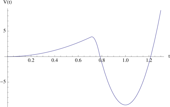
Figure 1: The potential for $\mu_{1}=1.1$, $\bar{\mu}_{2}=10.1$, $\mu_{3}=5.1$ and $t_{M}=0.715$ ($k=0$).

3.1 The solution for $T=0$

The scalar equation of motion (2.7) for the background solution $t_{b}(z)$ simplifies to

$$z^{2}\,t_{b}^{\prime\prime}(z)-(d-1)z\,t_{b}^{\prime}(z)-A\,t_{b}(z)=B$$ (3.15)

The solution to (3.15) we are looking for can be written as

$$t_{b}(z)=\left\{\begin{array}[]{lcr}t_{1}\;(z/z_{1})^{\Delta_{1}^{+}}&,&0<z<z_{1}\\ t_{M}+D_{+}\,(z/z_{2})^{\Delta_{2}^{+}}+D_{-}\,(z/z_{2})^{\Delta_{2}^{-}}&,&z_{1}<z<z_{2}\\ 1-(1-t_{2})\,(z/z_{2})^{\Delta_{3}^{-}}&,&z_{2}<z<\infty\end{array}\right.$$ (3.16)

From the continuity of the solution and its derivative at $z_{1,2}$ we get four equations. In principle they should determine the four unknowns $D_{+,-}$ and $z_{1,2}$, but due to dilatation invariance $z\to\lambda z$ of (3.15) only the ratio $z_{2}/z_{1}>1$ appears. It is straightforward to show that in spite of this, a solution is still possible for a special, quantized choice

$$d\,\bar{\mu}_{2}\,\ln{(z_{2}/z_{1})}=(2\,k+1)\;\pi-\alpha_{1}-\alpha_{3}\qquad;\qquad k=0,1,2,\dots$$ (3.17)

where we used (3.13) and defined the phases

$$0<\alpha_{i}\equiv\arctan\frac{\bar{\mu}_{2}}{\mu_{i}}<\frac{\pi}{2}\quad,\quad i=1,3$$ (3.18)

This then leads to a quantized relation among the potential parameters $t_{M}$, $\mu_{1,3}$ and $\bar{\mu}_{2}$:

$$t_{M}^{(k)}=\left(1+\frac{\mu_{1}+1/2}{\mu_{3}-1/2}\;\left(\frac{\mu_{3}^{2}+\bar{\mu}_{2}^{2}}{\mu_{1}^{2}+\bar{\mu}_{2}^{2}}\right)^{1/2}\exp{\left(\frac{(2k+1)\pi-\alpha_{1}-\alpha_{3}}{2\,\bar{\mu}_{2}}\right)}\right)^{-1}$$ (3.19)

As we anticipated, solutions to our system of equations exist only for special discrete values of the model parameter $t_{M}$. Not all $k$ are however allowed for the solution (3.16). In fact, what can happen is that the solution as a function of $z$ instead of increasing starts decreasing (or oscillating) at some point. This may lead to a change of the region of the piecewise potential, so that in such a case more intervals in $z$ should be included for the solution.

As an example, we can take $\mu_{1}=1.1$, $\bar{\mu}_{2}=10.1$, $\mu_{3}=5.1$ and $k=0$. The output parameters are given by $z_{2}/z_{1}=1.014$, $t_{1}=0.708$, $t_{M}=0.715$ and $t_{2}=0.772$. The solution with $z_{1}=1$ is shown in fig. 2. The ansatz (3.16) is consistent also for $k=1,2$, but not for $k>2$. In that case one should add one or more $z$-intervals.

Finally, from $(\ref{bb})$, $(\ref{vev})$ and (3.16) we read the vev of the order parameter signalling the spontaneous breakdown of the discrete symmetry,

$$<\hat{O}>\;=\;\frac{2\,d\,\mu_{1}\,\phi_{m}}{L\,z_{1}^{\Delta_{1}^{+}}}\,t_{1}$$ (3.20)

More about correlation functions will be discussed in Section 4.

3.2 The solution for $T\neq 0$

The equation of motion (2.7) for $z_{h}=1$ takes the form,

$$(1-z^{d})\;z^{2}\;t_{b}^{\prime\prime}(z)-(d-1+z^{d})\;z\;t_{b}^{\prime}(z)-A\;t_{b}(z)=B$$ (3.21)

Two independent solutions of the homogeneous part exist in any region,

$$t_{\mu}^{\pm}(z)=z^{d(1/2\pm\mu)}\;F\left(\frac{1}{2}\pm\mu,\frac{1}{2}\pm\mu;1\pm 2\mu;z^{d}\right)$$ (3.22)

where $\mu$ is as in (3.14) and $F\left(a,b;c;z\right)={}_{2}F_{1}\left(a,b;c;z\right)$ is the standard hypergeometric function. For $z\in[0,1]$, both solutions (3.22) are real for $\mu\in\mathbb{R}$, and conjugate-related for $\mu\in i\,\mathbb{R}$.

For $z\to 0$ they behave as

$$t_{\mu}^{\pm}(z)\to\;z^{\Delta_{\pm}}\;\left(1+{\cal O}(z^{d})\right)$$ (3.23)

So in the small $z$ region (near the boundary) only $t_{\mu_{1}}^{+}(z)$ is admissible, i.e. the one that drops as $\Delta_{1}^{+}$.

The behavior for $z\to 1^{-}$ is on the other side like,

$$t_{\mu}^{\pm}(z)\to-\frac{\Gamma(1\pm 2\,\mu)}{\Gamma(\frac{1}{2}\pm\mu)^{2}}\;\ln{(1-z)}+{\cal O}(1)$$ (3.24)

Neither of them is admissible close to the horizon at $z=1$ but it is so the obvious linear combination that can be chosen,

$$Q_{\mu_{3}}(z)\equiv\frac{\Gamma(1-2\mu_{3})}{\Gamma(\frac{1}{2}-\mu_{3})^{2}}\;t_{\mu_{3}}^{+}(z)-\frac{\Gamma(1+2\mu_{3})}{\Gamma(\frac{1}{2}+\mu_{3})^{2}}\;t_{\mu_{3}}^{-}(z)$$ (3.25)

To closely follow the $T=0$ case, we write the solution in the form,

$$t_{b}(z)=\left\{\begin{array}[]{lcl}t_{1}\;\frac{t_{\mu_{1}}^{+}(z)}{t_{\mu_{1}}^{+}(z_{1})}&\quad,&0<z<z_{1}\\ t_{M}+D_{+}\;t_{\mu_{2}}^{+}(z)+D_{-}\;t_{\mu_{2}}^{-}(z)&\quad,&z_{1}<z<z_{2}\\ 1-(1-t_{2})\;\frac{Q_{\mu_{3}}(z)}{Q_{\mu_{3}}(z_{2})}&\quad,&z_{2}<z<1\end{array}\right.$$ (3.26)

There is no dilatation symmetry here, so the number of unknowns $(D_{+},D_{-},z_{1},z_{2})$ matches the number of equations from continuity of the solution and its derivative at $z=z_{1}$ and $z=z_{2}$. We expect to find the solution for continuous choices of the model parameters $A_{1,2,3}$, $t_{M}$. Notice that at $T=0$ the input were $A_{1,2,3}$ and a flat direction $z_{1}$.

As an example we can consider the same input parameters that we used in the $T=0$ case: $\mu_{1}=1.1$, $\bar{\mu}_{2}=10.1$, $\mu_{3}=5.1$. Instead of $z_{1}$, which is now an output rather than an input, we choose the same $t_{M}$ as before, i.e. $t_{M}=0.715$ (at $T=0$ this was an output). The corresponding solution gives $z_{1}=0.2$, $z_{2}=0.203$, $t_{1}=0.708$, $t_{2}=0.772$, resulting into a positive action integral $I[t_{b}]=1.184$. The solution plot is given in fig. 2.

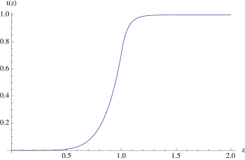
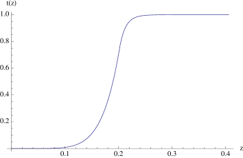
Figure 2: The solution for $T=0$ (left) and $T\neq 0$ (right) for $\mu_{1}=1.1$, $\bar{\mu}_{2}=10.1$, $\mu_{3}=5.1$, $t_{M}=0.715$ ($k=0$). The $T=0$ (massless) wall has been chosen to start at $z_{1}=1$, but can be freely translated to the left or right.

For $T\neq 0$ the allowed region is only $z\in[0,1]$, while for $T=0$ it is $z\in[0,\infty]$. The solutions for the domain wall close to the boundary $z=0$ are very similar in the two cases, with the differences hardly noticeable. On the contrary, when the domain wall goes towards larger values (close to $z=1$ or bigger) the differences become more and more evident. It is worth stressing that although at finite temperature the position of the domain wall is fixed by the initial choice of the potential parameters (i.e. both $z_{1}$ and $z_{2}$ are determined by the continuity of the solution), this is no longer true for vanishing temperature, where only the ratio $z_{2}/z_{1}$ can be evaluated and thus the domain wall position is undetermined. In any case a fundamental difference between the two cases is, as we already mentioned, the value of the action (free energy): vanishing for $T=0$ and positive for $T>0$, in accord with (2.16).

Finally, from $(\ref{bb})$, $(\ref{vev})$ and (3.26) we read the vev of the order parameter signaling the spontaneous breakdown of the discrete symmetry in this metastable phase,

$$<\hat{O}>\;=\;\frac{2\,d\,\mu_{1}\,\phi_{m}}{L\,t^{+}_{\mu_{1}}(z_{1})}\,t_{1}$$ (3.27)

4 About correlation functions

Having an exact solution, we can try to analytically compute the correlation functions of the boundary theory.

The derivatives of the potential (3.1), (3.8) are

$$V^{\prime}(t) = \left\{\begin{array}[]{l}A_{1}\,t\\ A_{2}\,(t-t_{M})\\ A_{3}\,(t-1)\end{array}\right.\qquad;\qquad V^{\prime\prime}(t)=\left\{\begin{array}[]{l}A_{1}>0\\ A_{2}<0\\ A_{3}>0\end{array}\right.$$ (4.7)

$$V^{(n+3)}(t) = (A_{2}-A_{1})\,\delta^{(n)}(t-t_{1})+(A_{3}-A_{2})\,\delta^{(n)}(t-t_{2})\quad,\quad n=0,1,\ldots$$

which will be used in the expansion

$$V^{\prime}(t_{b}+\xi)=\sum_{n=0}^{\infty}\frac{1}{n!}\;V^{(n+1)}(t_{b})\;\xi^{n}$$ (4.8)

To compute correlation functions we refer the reader to the formalism sketched in Appendix B. The equation of motion for a general field $t(x,z)$ is (B.1) and the solution is searched perturbatively via (B.4)-(B.13). According to (B.16) the $m$-th approximation behaves as

$$z\to 0\quad:\quad\xi^{(m)}(x,z)\to\xi_{(0)}(x)\;z^{\Delta_{-}}\;\delta_{m,1}+\xi_{(1)}^{(m)}(x)\;z^{\Delta_{+}}+\ldots$$ (4.9)

with $\xi_{(1)}^{(m)}$ a functional of $\xi_{(0)}$. Now, from equations (2.12), (B.4), (B.7),

$$<\hat{O}(x)>_{\phi_{(0)}}=\frac{\Delta_{+}-\Delta_{-}}{L}\;\phi_{(1)}(x)=\frac{2\,\nu_{1}\,\phi_{m}}{L}\;\left(t_{b}{}_{(1)}+\sum_{m=1}^{\infty}\xi^{(m)}_{(1)}(x)\right)$$ (4.10)

where we introduced from the region $z\to 0$

$$\nu_{1}=d\,\mu_{1}=\frac{\Delta_{+}-\Delta_{-}}{2}$$ (4.11)

From here the result used so far (see (3.20), (3.27)) follows

$$<\hat{O}(x)>=\frac{2\,\nu_{1}\,\phi_{m}}{L}\;t_{b}{}_{(1)}$$ (4.12)

For $n>1$ we have from (4.10) and (B.22),

$$<\hat{O}(x_{1})\dots\hat{O}(x_{n})>=\frac{2\,\nu_{1}}{L\,\phi_{m}{}^{n-2}}\;\frac{\delta^{n-1}\,\xi^{(n-1)}_{(1)}(x_{1})}{\delta\xi_{(0)}(x_{2})\dots\delta\xi_{(0)}(x_{n})}$$ (4.13)

In the following we will specialize to the $T=0$ case.

4.1 The 2-point correlator

Defining the momentum space first order perturbations through

$$\xi^{(1)}(x,z)\equiv\int\frac{d^{d}k}{(2\pi)^{d}}\;e^{ik\cdot x}\;\tilde{\xi}^{(1)}(k,z)$$ (4.14)

equation (B.12) for $\tilde{\xi}^{(1)}$ becomes ($\hat{k}\equiv L\,\sqrt{k^{2}}$, $f^{\prime}\equiv\partial f/\partial z$)

$$z^{2}\,\tilde{\xi}^{(1)}{}^{\prime\prime}(k,z)-(d-1)\,z\,\tilde{\xi}^{(1)}{}^{\prime}(k,z)-\left(\hat{k}^{2}\,z^{2}+V^{\prime\prime}(t_{b})\right)\,\tilde{\xi}^{(1)}(k,z)=0$$ (4.15)

with $V^{\prime\prime}(t_{b})=A_{i}$ for $i=1,2,3$ depending on the region. The solution is

$$\tilde{\xi}^{(1)}(k,z)=z^{\frac{d}{2}}\left\{\begin{array}[]{lcr}A(k)\;\;K_{\nu_{1}}(\hat{k}z)+B(k)\;I_{\nu_{1}}(\hat{k}z)&,&0\leq z<z_{1}\\ C(k)\;I_{i\bar{\nu}_{2}}(\hat{k}z)+C^{*}(k)\;I_{-i\bar{\nu}_{2}}(\hat{k}z)&,&z_{1}<z<z_{2}\\ D(k)\;K_{\nu_{3}}(\hat{k}z)&,&z_{2}<z<\infty\end{array}\right.$$ (4.16)

where $A(k)$ is normalized by (4.9) to be

$$A(k)=\frac{\hat{k}^{\nu}}{2^{\nu-1}\,\Gamma(\nu)}\tilde{\xi}_{(0)}(k)$$ (4.17)

The coefficients $B(k),C(k)$ and $D(k)$ are determined by imposing continuity of $\tilde{\xi}^{(1)}(k,z)$ and its derivative at $z=z_{1},z_{2}$. All we need for our purpose is

$$\frac{B(k)}{A(k)}=-\;\frac{Im\left[w(K_{\nu_{1}},I_{i\bar{\nu}_{2}};\hat{k}z_{1})w(K_{\nu_{3}},I_{-i\bar{\nu}_{2}};\hat{k}z_{2})\right]}{Im\left[w(I_{\nu_{1}},I_{i\bar{\nu}_{2}};\hat{k}z_{1})w(K_{\nu_{3}},I_{-i\bar{\nu}_{2}};\hat{k}z_{2})\right]}$$ (4.18)

where

$$w(f,g;x)\equiv f(x)\,g^{\prime}(x)-g(x)\,f^{\prime}(x)$$ (4.19)

denotes the Wronskian of $f$ and $g$ at $x$. The normalization (4.17) determines the coefficient of $z^{\Delta_{1}^{-}}$ in the expansion of (4.16) for $z\rightarrow 0$ to be $\tilde{\xi}_{(0)}(k)$, while the coefficient of $z^{\Delta_{1}^{+}}$ is

$$\tilde{\xi}^{(1)}_{(1)}(k)=-\frac{\Gamma(1-\nu_{1})}{\Gamma(1+\nu_{1})}\,\frac{\hat{k}^{2\nu_{1}}}{2^{2\nu_{1}}}\;\left(1-\frac{2}{\Gamma(\nu_{1})\,\Gamma(1-\nu_{1})}\,\frac{B(k)}{A(k)}\right)\;\tilde{\xi}_{(0)}(k)$$ (4.20)

Finally, the two-point function can be calculated from (4.13):

$$<\hat{O}(x_{1})\hat{O}(x_{2})>=\frac{2\,\nu_{1}}{L}\;\frac{\delta\,\xi^{(1)}_{(1)}(x_{1})}{\delta\xi_{(0)}(x_{2})}$$ (4.21)

Defining the Fourier transform

$$\langle\hat{O}(x_{1})\hat{O}(x_{2})\rangle=\int\frac{d^{d}k}{(2\pi)^{d}}e^{ik(x_{1}-x_{2})}G_{2}(k)$$ (4.22)

we get in our SSB solution case from (4.20)

$$G_{2}^{SSB}(k)=-\frac{2\,\nu_{1}}{L}\;\frac{\Gamma(1-\nu_{1})}{\Gamma(1+\nu_{1})}\,\frac{\hat{k}^{2\nu_{1}}}{2^{2\nu_{1}}}\;\left(1-\frac{2}{\Gamma(\nu_{1})\,\Gamma(1-\nu_{1})}\,\frac{B(k)}{A(k)}\right)$$ (4.23)

The second term in the parenthesis signals the deviation of the CFT. In fact in the conformal vacuum ($t_{b}=0$) the propagator reduces to the well known form

$$G_{2}(k)=-\frac{2\,\nu_{1}}{L}\;\frac{\Gamma(1-\nu_{1})}{\Gamma(1+\nu_{1})}\;\frac{\hat{k}^{2\nu_{1}}}{2^{2\nu_{1}}}\quad\longleftrightarrow\quad\langle\hat{O}(x_{1})\hat{O}(x_{2})\rangle=\frac{2\,\nu_{1}}{L}\;\frac{\Gamma(\Delta_{+}^{(1)})}{\pi^{\frac{d}{2}}\,\Gamma(\nu_{1})}\;\frac{1}{|x_{1}-x_{2}|^{2\,\Delta_{+}^{(1)}}}$$ (4.24)

Let us now analyze the propagator (4.23) in some limits.

We first expand (4.23) for small $k$ (IR limit). To calculate the numerator of (4.18), the leading terms of the Wronskians (4.19) are enough, but for the denominator these leading terms give zero due to the constraint (3.17), so that the next terms are needed. For $\nu_{3}>1$ (this is automatically true for $d>2$) the propagator has a pole,

$$k^{2}\to 0\quad:\quad G_{2}^{SSB}(k)\to\frac{8z_{1}^{-2\nu_{1}}\nu_{1}(1+\bar{\nu}_{2}^{2})}{(\nu_{1}^{2}+\bar{\nu}_{2}^{2})\left(\frac{1+\nu_{3}}{1-\nu_{3}}z_{2}^{2}-\frac{1-\nu_{1}}{1+\nu_{1}}z_{1}^{2}\right)}\frac{1}{\hat{k}^{2}}$$ (4.25)

and obviously a corresponding massless mode associated with it. This is the Goldstone mode associated to the SSB of the conformal invariance due to the vev deformation [9].

Finally, at large $k$, i.e. in the UV, the SSB propagator approaches exponentially fast the conformal one. The boundary QFT is thus conformal in the UV. What is relevant in this limit is just the parameter that determines the potential close to $\phi=0$, i.e. $\mu_{1}$ (or equivalently $A_{1}$) only.

The behavior of the propagator in the IR and UV is plotted on fig. 3.

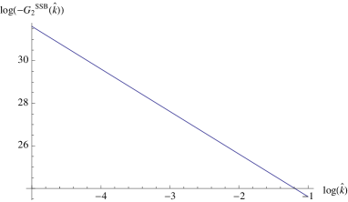
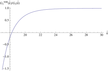
Figure 3: The behavior of the propagator in the SSB case for $T=0$ at small $\hat{k}$ (left) and large $\hat{k}$ (right) for $\mu_{1}=1.1$, $\bar{\mu}_{2}=10.1$, $\mu_{3}=5.1$, $t_{M}=0.715$ ($k=0$). Notice the zero of the propagator for $\hat{k}\approx 18.25$.

Notice that the choice of $z_{1}$, which is not determined by the equation of motion, is arbitrary, but the different choices generate different boundary QFT (different correlators). The meaning of this $z_{1}$ is connected to the boundary in momentum space between the CFT in the UV region ($k>>1/z_{1}$) and the QFT of a massless mode in the IR region ($k<<1/z_{1}$). So it seems we have a continuous family of theories that interpolate between these two limits. The massless mode is a consequence of this flat direction: no energy is needed for the wall to move, so the excitation in this direction is cost-free, i.e. with vanishing eigenvalue.

4.2 The 3-point correlator

For the 3-point correlation function we need to compute $\tilde{\xi}^{(2)}(x,z)$ from (B.9). The solution for $m=2$ in (B.20) reduces to

$$\xi^{(2)}(x,z)=\int d^{d}x^{\prime}dz^{\prime}\sqrt{det\,g_{ab}}\;G(x,z;x^{\prime},z^{\prime})\;\frac{1}{2}\;V^{(3)}(t_{b}(z^{\prime}))\;\left(\xi^{(1)}(x^{\prime},z^{\prime})\right)^{2}$$ (4.26)

where $G(x,z;x^{\prime},z^{\prime})$ is the bulk-bulk propagator. Fortunately we do not need to compute it, since the relevant part is just the $z^{\Delta_{+}}$ coefficient of $\xi^{(2)}(x,z)$ in the small $z$ expansion,

$$z\to 0\quad:\quad G(x,z;x^{\prime},z^{\prime})\to\frac{1}{2\,\nu_{1}\,L}\;z^{\Delta_{1}^{+}}\;K(x^{\prime},z^{\prime};x)$$ (4.27)

where we introduced the bulk-boundary propagator

$$K(x,z;x^{\prime})=\int\frac{d^{d}k}{(2\pi)^{d}}\;e^{ik\cdot(x-x^{\prime})}\;K(k,z)\quad,\quad K(k,z)=\frac{\tilde{\xi}^{(1)}(k,z)}{\tilde{\xi}_{(0)}(k)}$$ (4.28)

Using (B.18) and (4.13) we get

$$\langle\hat{O}(x_{1})\;\hat{O}(x_{2})\;\hat{O}(x_{3})\rangle=\frac{1}{L^{2}\,\phi_{m}}\;\int d^{d}x\,\int dz\,\sqrt{\det g_{ab}}\;V^{(3)}(t_{b}(z))\;\prod_{i=1}^{3}\,K(x,z;x_{i})$$ (4.29)

This same result could have been of course derived from Witten’s diagrams recipe.

The case of conformal vacuum would give here a vanishing 3-point function, as required by the unbroken $Z_{2}$ symmetry.

In our case we have from (4.7)

$$V^{(3)}(t_{b}(z)) = (A_{2}-A_{1})\;\delta(t_{b}(z)-t_{b}(z_{1}))+(A_{3}-A_{2})\;\delta(t_{b}(z)-t_{b}(z_{2}))$$ (4.30)

$$= \frac{(A_{2}-A_{1})}{\left|t_{b}^{\prime}(z_{1})\right|}\;\delta(z-z_{1})+\frac{(A_{3}-A_{2})}{\left|t_{b}^{\prime}(z_{2})\right|}\;\delta(z-z_{2})$$ (4.31)

The momentum space three-point correlation function from

$$\langle\hat{O}(x_{1})\;\hat{O}(x_{2})\;\hat{O}(x_{3})\rangle = \int\frac{d^{d}k_{1}}{(2\pi)^{d}}\int\frac{d^{d}k_{2}}{(2\pi)^{d}}\int\frac{d^{d}k_{3}}{(2\pi)^{d}}\;(2\pi)^{d}\;\delta^{d}(k_{1}+k_{2}+k_{3})$$ (4.32)

$$\times e^{ik_{1}x_{1}}\,e^{ik_{2}x_{2}}\,e^{ik_{3}x_{3}}\;G_{3}(k_{1},k_{2},k_{3})$$

remains thus without any integration:

$$L\;\phi_{m}\;G_{3}(k_{1},k_{2},k_{3}) = \frac{(A_{2}-A_{1})}{z_{1}^{d+1}\left|t_{b}^{\prime}(z_{1})\right|}\;K(k_{1},z_{1})\;K(k_{2},z_{1})\;K(k_{3},z_{1})$$ (4.33)

$$+ \frac{(A_{3}-A_{2})}{z_{2}^{d+1}\left|t_{b}^{\prime}(z_{2})\right|}\;K(k_{1},z_{2})\;K(k_{2},z_{2})\;K(k_{3},z_{2})$$ (4.34)

The 3-point correlator has the right poles for $k_{i}^{2}=0$, as it should due to the presence of the massless asymptotic state.

5 Discussion and conclusions

In this paper we have assumed that the tree level approximation is good enough. In fact here, contrary to what happens in some string theory constructions, we do not have any large $N$ argument for this to be true. What we did was just to solve perturbatively the classical bulk equation of motion with sources, which, by definition, gives the tree order generating functional for connected diagrams. The next step would be to consider loops, which is far beyond the scope of this paper. Notice however that this situation is similar to most models of superconductivity that have appeared in the literature in recent years.

Another approximation we used is $\kappa\to 0$, i.e. no back-reaction. Once back-reaction (finite $\kappa$) is introduced, no exactly solvable solutions are known, and only numerical analysis can be applied. Of course in such a case considering a piece-wise quadratic potential is no more needed, since analytic results are anyway unavailable. On the other side, although we will not attempt to do it here, there is hope to attack some issues in the back-reacted system even without demanding numerical work. Namely, one could try to calculate the action along the lines of subsection 2.2 and appendix A and check whether the free energy gets lifted or not. Similar studies can be found in the literature, for example [11], where BPS type domain walls solutions in gauged supergravity context were considered. We remark that the non trivial solutions analyzed in this paper are not domain walls that describe renormalization group flows driven by deformation of the CFT by a relevant operator; they describe the CFT just in a non conformal vacuum.

We found out that the $Z_{2}$ symmetry breaking and preserving vacua are both equally possible at $T=0$. The two phases can be co-existent, since they have the same free energy. This behavior changes at non-zero (high) temperature. Although there exists a non-trivial solution also in this case, the free energy associated with this SSB vacuum is higher than the trivial (symmetry preserving) one. This system thus seems to prefer symmetry restoration at high temperature. It is however interesting that in many systems the non trivial phase disappears with the transition (for example in [5], [12]), but not here neither in [13] where examples from holographic models of superconductors derived from gauged supergravity are given. It is thus reasonable to interpret this non-trivial solution at $T>0$ found here as describing a metastable phase of symmetry non-restoration at high temperature [14, 15], see for example [16] for a review on this subject.

For the case $T=0$ we noticed that dilatation symmetry leads to a curious behavior: in order to get a non-trivial solution to the equations of motion, a relation among the parameters of the potential is needed to be satisfied. Although this means a strange fine-tuning for the bulk parameters, it has a physical effect for the boundary theory, i.e. a massless mode. The existence of this mode is a consequence of dilatation symmetry: changing the position of the domain wall between the two vacua costs no energy, and the quantum mechanical excitation connected is obviously massless. In other words, dilatation symmetry is global, and the position of the wall breaks it spontaneously. The massless mode is thus the Goldstone originating from it, i.e. the dilaton. Then one would expect the propagator at $T\neq 0$ not to have a pole at $k^{2}=0$, since there is no symmetry to start with. Although we were unable to solve the equations for the perturbations analytically in this case, the absence of a pole seems reasonable: there is no constraint (3.19) at $T\neq 0$, so no reason to expect a magic cancelation of the leading term in $k^{2}\to 0$ of the denominator in (4.18).

The analysis of the previous section showed that in the UV ($k\to\infty$) limit the calculated correlation functions approach their correspondent correlation functions of the conformal vacuum. What gets corrected is the opposite, IR limit. And the theory here is a strongly interacting theory of a massless mode.

In this paper we limit ourselves to the 1, 2 and 3-point correlation functions. This is mainly due to simplicity. Higher point correlation functions can be studied in a similar fashion, but involve the use of the bulk-bulk propagator, which, although straightforward, is a bit more involved. Also, two particular situations were avoided in this paper. One is the case of integer $\nu_{1}$, which gives logarithmic corrections that complicate the analysis. The other case is $\nu_{1}$ in the conformal window [7, 17], for which both $\Delta_{\pm}$ are positive. We plan to cover these and related topics in a follow-up publication.

Appendix A Derivation of equation $(\ref{actionfinal})$

Since we believe that (2.16) is not completely obvious, we present a short derivation of it.

We want to simplify the expression for the action

$$I[t]\equiv\int_{0}^{z_{h}}\frac{dz}{z^{d+1}}\left(\frac{z^{2}}{2}(1-(z/z_{h})^{d})t^{\prime 2}(z)+V(t(z))\right)$$ (A.1)

for the solutions of the e.o.m. For them we can replace one $z\,t^{\prime}(z)$ above from the equation of motion

$$z\,t^{\prime}=\frac{1}{d-1}\;\left((1-(z/z_{h})^{d})\;z^{2}\;t^{\prime\prime}-V^{\prime}(t)-(z/z_{h})^{d}\;z\;t^{\prime}\right)$$ (A.2)

Then the first term in (A.1) can be rewritten as

$$\int_{0}^{z_{h}}\frac{dz}{z^{d+1}}\;\frac{z^{2}}{2}(1-(z/z_{h})^{d})\;t^{\prime 2}$$ (A.3)

$$= \int_{0}^{z_{h}}\frac{dz}{z^{d+1}}\;\frac{(1-(z/z_{h})^{d})}{2\,(d-1)}\;z\;t^{\prime}\;\left((1-(z/z_{h})^{d})\;z^{2}\;t^{\prime\prime}-V^{\prime}(t)-(z/z_{h})^{d}\;z\;t^{\prime}\right)$$ (A.4)

$$= \int_{0}^{z_{h}}dz\;\frac{(1-(z/z_{h})^{d})^{2}}{2\,(d-1)\,z^{d-2}}\;\left(\frac{t^{\prime 2}}{2}\right)^{\prime}-\int_{0}^{z_{h}}dz\;\frac{(1-(z/z_{h})^{d})}{2\,(d-1)\,z^{d}}\;\frac{dV}{dz}$$ (A.5)

$$- \int_{0}^{z_{h}}dz\;\frac{(z/z_{h})^{d}\,(1-(z/z_{h})^{d})}{2\,(d-1)\,z^{d-1}}\;t^{\prime 2}$$ (A.6)

$$= \left(\frac{(1-(z/z_{h})^{d})^{2}}{2\,(d-1)\,z^{d-2}}\;\frac{t^{\prime 2}}{2}\right)_{0}^{z_{h}}-\int_{0}^{z_{h}}dz\;\frac{d}{dz}\left(\frac{(1-(z/z_{h})^{d})^{2}}{2\,(d-1)\,z^{d-2}}\right)\;\frac{t^{\prime 2}}{2}$$ (A.7)

$$- \left(\frac{1-(z/z_{h})^{d}}{2\,(d-1)\,z^{d}}\;V(t)\right)_{0}^{z_{h}}+\int_{0}^{z_{h}}dz\;\frac{d}{dz}\left(\frac{(1-(z/z_{h})^{d})}{2\,(d-1)\,z^{d}}\right)V(t)$$ (A.8)

$$- \int_{0}^{z_{h}}dz\;\frac{(z/z_{h})^{d}\,(1-(z/z_{h})^{d})}{2\,(d-1)\,z^{d-1}}\;t^{\prime 2}$$ (A.9)

where we used $t^{\prime}dV/dt=dV/dz$ and integration by parts. By rearranging and simplifying (A.3) we get the following identity for any solution of the equation of motion $t(z)$:

$$d\,\int_{0}^{z_{h}}\;\frac{dz}{2\,z^{d-1}}\;(1-(z/z_{h})^{d})^{2}\;t^{\prime 2}$$ (A.10)

$$= \left[\frac{1-(z/z_{h})^{d}}{z^{d}}\;\left(\frac{z^{2}}{2}\;(1-(z/z_{h})^{d})\;t^{\prime 2}-V(t)\right)\right]_{z=0}^{z=z_{h}}-d\,\int_{0}^{z_{h}}\;\frac{dz}{z^{d+1}}\;V(t)$$ (A.11)

Since

$$(1-(z/z_{h})^{d})^{2}=(1-(z/z_{h})^{d})-(z/z_{h})^{d}\;(1-(z/z_{h})^{d})$$ (A.12)

we get finally

$$I[t_{b}] = \left[\frac{(1-(z/z_{h})^{d})}{d\,z^{d}}\left(\frac{z^{2}}{2}\;(1-(z/z_{h})^{d})\;t_{b}^{\prime 2}-V(t_{b})\right)\right]_{z=0}^{z=z_{h}}$$ (A.13)

$$+ \frac{1}{2}\int_{0}^{z_{h}}dz\;(z/z_{h})^{d}\;\frac{1-(z/z_{h})^{d}}{z^{d-1}}\;t_{b}^{\prime 2}$$ (A.14)

for any solution to the equation of motion $t_{b}(z)$, which is nothing else than (2.16).

Appendix B Formalism to compute correlation functions

According to (2.11), to compute arbitrary $m$-points correlation functions we must obtain a solution to the equation of motion

$$0 = D^{2}(\phi)-U^{\prime}(\phi)\equiv\frac{\phi_{m}}{L^{2}}\;E[t]$$ (B.1)

$$E[t] = (1-(z/z_{h})^{d})\;z^{2}\;t^{\prime\prime}(x,z)-(d-1+(z/z_{h})^{d})\;z\;t^{\prime}(x,z)$$ (B.2)

$$+ L^{2}\;z^{2}\;\left(\frac{1}{1-(z/z_{h})^{d}}\,\partial^{2}_{\tau}t(x,z)+\nabla^{2}t(x,z)\right)-V^{\prime}(t)$$ (B.3)

with arbitrary boundary value $t(x,0)$ but finite $t(x,z_{h})$. To this end we take the following route:

• We consider

  $$t(x,z)=t_{b}(z)+\xi(x,z)$$ (B.4)

  with $t_{b}(z)$ the background field solution of (2.7) dual to the boundary QFT. The following expansion holds ($T=0$),

  $$E[t_{b}+\xi] = \hat{L}[t_{b}]\xi-\sum_{n=2}^{\infty}\,\frac{1}{n!}V^{(n+1)}(t_{b})\,\xi^{n}$$ (B.5)

  $$\hat{L}[t_{b}]\xi \equiv \left(z^{2}\,\partial_{z}^{2}-(d-1)\,z\,\partial_{z}+L^{2}\,z^{2}\,\Box_{x}-V^{\prime\prime}(t_{b}(z))\right)\,\xi(x,z)$$ (B.6)

• We introduce the expansion,

  $$\xi(x,z)\equiv\sum_{m=1}^{\infty}\,\lambda^{m}\,\xi^{(m)}(x,z)$$ (B.7)

  where the parameter $\lambda$ is just to count powers and will be set to one at the end.

• We merge this expansion in the functional $E[t_{b}+\xi]$; we get,

  $$E[t_{b}+\xi]=E[t_{b}+\sum_{m=1}^{\infty}\,\lambda^{m}\,\xi^{(m)}]\equiv\sum_{m=1}^{\infty}\lambda^{m}\;E^{(m)}[\xi^{(1)},\dots,\xi^{(m)};t_{b}]$$ (B.8)

  where for the first three terms,

  $$E^{(1)}[\xi^{(1)};t_{b}] = \hat{L}[t_{b}]\xi^{(1)}$$ (B.9)

  $$E^{(2)}[\xi^{(1)},\xi^{(2)};t_{b}] = \hat{L}[t_{b}]\xi^{(2)}-\frac{1}{2}V^{(3)}(t_{b})\,\left(\xi^{(1)}\right)^{2}$$ (B.10)

  $$E^{(3)}[\xi^{(1)},\xi^{(2)},\xi^{(3)};t_{b}] = \hat{L}[t_{b}]\xi^{(3)}-V^{(3)}(t_{b})\,\xi^{(1)}\,\xi^{(2)}-\frac{1}{6}V^{(4)}(t_{b})\,\left(\xi^{(1)}\right)^{3}$$ (B.11)

• We ask for (B.4) to be a solution to the equation of motion, i.e. $r.h.s.(\ref{expaneq})=0$, by imposing $E^{(m)}=0$ for all $m$. That is, we first solve,

  $$\hat{L}[t_{b}]\xi^{(1)}=0$$ (B.12)

  and successively,

  $$\hat{L}[t_{b}]\xi^{(m)}=J^{(m)}[x,z;\xi^{(1)},\dots,\xi^{(m-1)};t_{b}]\quad,\quad m=2,3,\dots$$ (B.13)

  where the sources $J^{(m)}$ are read from (B.8) , for $m=1,2,3$ explicitly from (B.9).

To solve the system we must impose the following boundary conditions: for $z\rightarrow 0$ on the background solution they are,

$$t_{b}(z)\rightarrow t_{v}+t_{b}{}_{(1)}\,z^{\Delta_{+}}+\dots$$ (B.14)

where $t_{v}$ is a critical point of the potential, while that for the perturbation,

$$\xi(x,z)\rightarrow\xi_{(0)}(x)\,z^{\Delta_{-}}+\dots+\xi_{(1)}(x)\,z^{\Delta_{+}}+\dots$$ (B.15)

where $\xi_{(0)}(x)$ is a fixed, but arbitrary source. This will be implemented in the field expansion for $z\to 0$ as

$$z^{-\Delta_{-}}\,\xi^{(1)}(x,z)\rightarrow\xi_{(0)}(x)\qquad;\qquad z^{-\Delta_{-}}\,\xi^{(m)}(x,z)\rightarrow 0\quad,\quad m=2,3,\dots$$ (B.16)

Furthermore, at the horizon $z\to z_{h}$ we should ask that,

$$z^{-\Delta_{-}}\,\xi^{(m)}(x,z)<\infty\qquad,\qquad m=1,2,\dots$$ (B.17)

When $T=0$ the horizon is at $z_{h}=\infty$ and this condition enforces $\xi$ to go to zero fast enough. When $T>0$ the horizon is at $z=z_{h}=1$ and so this is just a finiteness condition for the $\xi^{(m)}$’s, i.e. for $\xi$.

Equation (B.12) is solved by,

$$\xi^{(1)}(x,z)=\int_{M_{d}}\;d^{d}x^{\prime}\;K(x,z;x^{\prime})\;\xi_{(0)}(x^{\prime})$$ (B.18)

where the bulk-boundary propagator matrix $K$ obeys,

$$\hat{L}[t_{b}]\,K(x,z;x^{\prime})=0\qquad;\qquad K(x,z;x^{\prime})\longrightarrow z^{\Delta_{-}}\;\delta^{d}(x,x^{\prime})\quad,\quad z\rightarrow 0$$ (B.19)

For $m>1$ instead, equations (B.13) are not homogeneous and we can write the solution in the way,

$$\xi^{(m)}(x,z)=\int\;d^{d}x^{\prime}\,dz^{\prime}\,\sqrt{\det g_{ab}}\;G(x,z;x^{\prime},z^{\prime})\;J^{(m)}(x^{\prime},z^{\prime})$$ (B.20)

where the bulk-bulk propagator $G$ obeys,

$$\hat{L}[t_{b}]\,G(x,z;x^{\prime},z^{\prime})=\delta_{g}^{d+1}(x,z;x^{\prime},z^{\prime})\qquad;\qquad z^{-\Delta_{-}}\;G(x,z;x^{\prime},z^{\prime})\longrightarrow 0\quad,\quad z\rightarrow 0$$ (B.21)

Now, from (B.18) it is obvious that $\xi^{(1)}$ is linear in $\xi_{(0)}$. Also, direct inspection of (B.20) shows that the following key property holds,

$$\xi^{(m)}\propto\left(\xi_{(0)}\right)^{m}\quad,\quad m=1,2,\dots$$ (B.22)

With all this baggage we can return to our task of computing the $m$-point correlation functions of $\phi(x,z)=\phi_{m}\,t(x,z)$. From (4.9), (4.10) and (B.22) we get,

$$<\hat{O}(x_{1})\dots\hat{O}(x_{m})>=\frac{2\,\nu_{1}}{L}\frac{\delta^{m}\varphi_{(1)}^{(m-1)}(x_{1})}{\delta\varphi_{(0)}(x_{2})\ldots\delta\varphi_{(0)}(x_{m})}$$ (B.23)

This procedure generates formally the well-known “Witten diagrams”, and can be straightforwardly extended to any QFT defined by its gravity dual.

References

- [1] J. M. Maldacena, “The large N limit of superconformal field theories and supergravity,” Adv. Theor. Math. Phys. 2, 231 (1998) [Int. J. Theor. Phys. 38, 1113 (1999)] [arXiv:hep-th/9711200].
- [2] S. S. Gubser, I. R. Klebanov and A. M. Polyakov, “Gauge theory correlators from non-critical string theory,” Phys. Lett. B 428, 105 (1998) [arXiv:hep-th/9802109].
- [3] E. Witten, “Anti-de Sitter space and holography,” Adv. Theor. Math. Phys. 2, 253 (1998) [arXiv:hep-th/9802150].
- [4] See for example, E. D’Hoker and D. Z. Freedman, “Supersymmetric gauge theories and the AdS / CFT correspondence,” hep-th/0201253, and references therein.
- [5] S. A. Hartnoll, C. P. Herzog and G. T. Horowitz, “Building a Holographic Superconductor,” Phys. Rev. Lett. 101, 031601 (2008) [arXiv:0803.3295 [hep-th]].
- [6] For a review see for example, S. A. Hartnoll, “Lectures on holographic methods for condensed matter physics,” Class. Quant. Grav. 26, 224002 (2009) [arXiv:0903.3246 [hep-th]]; J. McGreevy, “Holographic duality with a view toward many-body physics,” Adv. High Energy Phys. 2010, 723105 (2010) [arXiv:0909.0518 [hep-th]].
- [7] P. Breitenlöhner and D. Z. Freedman, “Stability in Gauged Extended Supergravity,” Annals Phys. 144 (1982) 249.
- [8] L. M. Krauss and F. Wilczek, “Discrete Gauge Symmetry in Continuum Theories,” Phys. Rev. Lett. 62 (1989) 1221; and references therein.
- [9] K. Skenderis, “Lecture notes on holographic renormalization,” Class. Quant. Grav. 19, 5849 (2002) [hep-th/0209067].
- [10] M. J. Duncan and L. G. Jensen, “Exact tunneling solutions in scalar field theory,” Phys. Lett. B 291, 109 (1992); G. Pastras, “Exact Tunneling Solutions in Minkowski Spacetime and a Candidate for Dark Energy,” arXiv:1102.4567 [hep-th]; K. Dutta, C. Hector, P. M. Vaudrevange and A. Westphal, “More Exact Tunneling Solutions in Scalar Field Theory,” Phys. Lett. B 708, 309 (2012) [arXiv:1110.2380 [hep-th]].
- [11] K. Skenderis and P. K. Townsend, “Gravitational stability and renormalization group flow,” Phys. Lett. B 468, 46 (1999) [hep-th/9909070].
- [12] A. R. Lugo, E. F. Moreno and F. A. Schaposnik, “Holographic Phase Transition from Dyons in an AdS Black Hole Background,” JHEP 1003 (2010) 013 [arXiv:1001.3378 [hep-th]]; “Holography and Self-Gravitating Dyons,” JHEP 1011 (2010) 081 [arXiv:1007.1482 [hep-th]].
- [13] F. Aprile, D. Roest and J. G. Russo, “Holographic Superconductors from Gauged Supergravity,” JHEP 1106, 040 (2011) [arXiv:1104.4473 [hep-th]].
- [14] S. Weinberg, “Gauge and Global Symmetries at High Temperature,” Phys. Rev. D 9 (1974) 3357.
- [15] R. N. Mohapatra and G. Senjanović, “Soft CP Violation at High Temperature,” Phys. Rev. Lett. 42 (1979) 1651; “Broken Symmetries at High Temperature,” Phys. Rev. D 20 (1979) 3390.
- [16] G. Senjanović, “Rochelle Salt: a Prototype of Particle Physics,” arXiv:hep-ph/9805361; B. Bajc, “High Temperature Symmetry Nonrestoration,” arXiv:hep-ph/0002187.
- [17] I. R. Klebanov and E. Witten, “AdS/CFT Correspondence and Symmetry Breaking,” Nucl. Phys. B 556 (1999) 89 [arXiv:hep-th/9905104].