A new code for parameter estimation in searches for gravitational waves from known pulsars

Abstract

We describe the consistency testing of a new code for gravitational wave signal parameter estimation in known pulsar searches. The code uses an implementation of nested sampling to explore the likelihood volume. Using fake signals and simulated noise we compare this to a previous code that calculated the signal parameter posterior distributions on both a grid and using a crude Markov chain Monte Carlo (MCMC) method. We define a new parameterisation of two orientation angles of neutron stars used in the signal model (the initial phase and polarisation angle), which breaks a degeneracy between them and allows more efficient exploration of those parameters. Finally, we briefly describe potential areas for further study and the uses of this code in the future.

matthew.pitkin@glasgow.ac.uk, colingill.glasgow@gmail.com, e.p.macdonald.glasgow@gmail.com, graham.woan@glasgow.ac.uk

1 Introduction

Over the last decade several searches have looked for gravitational waves from a large selection of known pulsars using data from the LIGO, GEO 600 and Virgo gravitational wave detectors [1, 2, 3, 4, 5, 6]. No evidence for signals has been observed, but these searches have produced upper limits on the gravitational wave amplitude for many pulsars by using Bayesian inference to calculate posterior probability distributions on the unknown signal parameters [7]. These searches have all assumed a single signal model in which the pulsars are triaxial and emit at precisely twice their rotational frequency, with the complex heterodyned and narrow-banded time domain signal described by

$$h(t)= h_{0}\left(\frac{1}{4}F_{+}(t,\psi)(1+\cos{}^{2}\iota)\cos{\phi_{0}}+\frac{1}{2}F_{\times}(t,\psi)\cos{\iota}\sin{\phi_{0}}\right)+$$

$$ih_{0}\left(\frac{1}{4}F_{+}(t,\psi)(1+\cos{}^{2}\iota)\sin{\phi_{0}}-\frac{1}{2}F_{\times}(t,\psi)\cos{\iota}\cos{\phi_{0}}\right),$$ (1)

where the four unknown parameters are the gravitational wave amplitude, $h_{0}$, polarisation angle, $\psi$, cosine of the inclination angle, $\cos{\iota}$ and the initial phase, $\phi_{0}$, and $F_{+}$ and $F_{\times}$ are the detector antenna patterns for the ’+’ and ’$\times$’ polarisations for the pulsar’s known sky position.

In early searches the posterior probability distribution was calculated on a 4-dimensional grid and the marginalisation integral required to produce posteriors on individual parameters was performed numerically using the trapezium rule. Later searches, which began allowing for inclusion of narrow uncertainties on extra signal parameters (such as frequency and sky position), performed the posterior exploration using a very basic Markov chain Monte Carlo (MCMC) method [5]. Both these methods, as applied in the search code, present practical implementation issues that mean they are not very flexible to all situations we may encounter: the former grid-based method quickly becomes computationally unworkable for larger parameters spaces, wastes time on posterior volumes with tiny probabilities and requires tuning of the grid for different strength signals; the MCMC method implemented was crude, required extensive tuning for certain signals and was not able to produce a Bayesian evidence value for model comparison (which could in the future be used as a detection statistic as in [9]).

Recently a new package of codes for Bayesian inference and evidence calculation (lalinference) have been created within the gravitational wave software repository lalsuite [10]. This suite contains more sophisticated MCMC methods (e.g. [11, 12]) and a method of Bayesian evidence calculation called nested sampling [13] that are able to more effectively explore posteriors without detailed tuning, can handle many parameters and provide values of the Bayesian evidence. We have used this new suite, and in particular its implementation of nested sampling (which can provide posterior probability distribution samples as well as an evidence value) to create a new code for the known pulsar search. Both new and old codes use the same likelihood as defined in [7], which assumes Gaussian noise with an its unknown variance analytically marginalised over.

This paper has two objectives: i) to show consistency between the new code and the previous code that has been used in astrophysical searches, and ii) to introduce a new parameterisation of two of the expected signal’s angular parameters, which breaks a degeneracy that leads to a bimodal posterior distribution. Finally, we briefly discuss how this new code will be used in future known pulsar searches.

2 The algorithm

Bayesian inference is underpinned by Bayes theorem, which for a problem defined by a set of variables $\vec{\theta}$, a dataset $d$ and some prior assumptions $I$, gives the posterior probability density

$$p(\vec{\theta}|d,I)=\frac{p(d|\vec{\theta},I)p(\vec{\theta})}{p(d|I)},$$ (2)

where $p(d|\vec{\theta},I)$ is the likelihood function, $p(\vec{\theta})$ is the prior probability distribution of the variables, and $p(d|I)$ is a normalising factor, often called the Bayesian evidence or the marginalised likelihood, which makes the total probability unity. The Bayesian evidence value can be very useful in testing different hypotheses on the same dataset i.e. models with different variables. It can be found by integrating, or marginalising, the numerator of eq:bayes over the prior ranges of all variables

$$Z=p(d,I)=\int_{\vec{\theta}}p(d|\vec{\theta},I)p(\vec{\theta}){\rm d}\vec{\theta}.$$ (3)

For many problems this integral will not be analytical, so numerical integration is required, which will become computationally unfeasible if calculating the integral on a grid for a large parameter space.

Nested sampling was developed [14] as an efficient method of performing the integral given by eq:evidence even for large parameter spaces. For good descriptions of the algorithm see [14, 13, 15]. As well as producing the evidence the routine will also output points sampled from the prior parameter volume and their associated likelihoods. These collected samples can be used to reconstruct the posterior probability distributions of the parameters.

3 Change of parameters

Other than the major change in the underlying algorithm used, a notable change that has been made in the new code is how it samples two of the signal’s angle parameters: the initial phase $\phi_{0}$ and the polarisation angle $\psi$. It is well known that these two parameters are degenerate to a $\pi/2$ radians shift in $\psi$ and $\pi$ radians shift in $\phi_{0}$ (see Figure 1). This issue can cause problems when trying to efficiently sample this parameter space. Within the nested sampling algorithm new samples are drawn by generating an MCMC with a proposal distribution calculated from the covariance of a set of previously sampled points. For a parameter that is circular about a particular prior range (e.g. an angle parameter wrapping round from $0$ to $2\pi$) circularity can be easily taken into account when calculating the covariance, but the degeneracy in the two mentioned parameters can lead to a bimodal distribution in $\phi_{0}$. This can be seen in Figure 1, for example with the signal represented by the blue circles. This bimodality will give a vastly distorted covariance matrix and lead to very low acceptance rates of new points within the MCMC sampling.

A way to avoid this is to find a new parameterisation in which both parameters are circular without causing any discontinuity and subsequent bimodality. Such a parameterisation is given by

$${\phi^{\prime}}_{0} =\phi_{0}\sin{\theta}+\psi\cos{\theta},$$

$$\psi^{\prime} =-\phi_{0}\sin{\theta}+\psi\cos{\theta},$$ (4)

where $\theta=\arctan{(1/2)}$. These new axes are shown by the dashed black lines in Figure 1. It can be seen that signals lying at the edges of this parameter space wrap around cleanly (the blue and red circles) at the edge of the ranges of $-(\pi/2)\cos{\theta}\leq{\phi^{\prime}}_{0},\psi^{\prime}\leq(\pi/2)\cos{\theta}$.

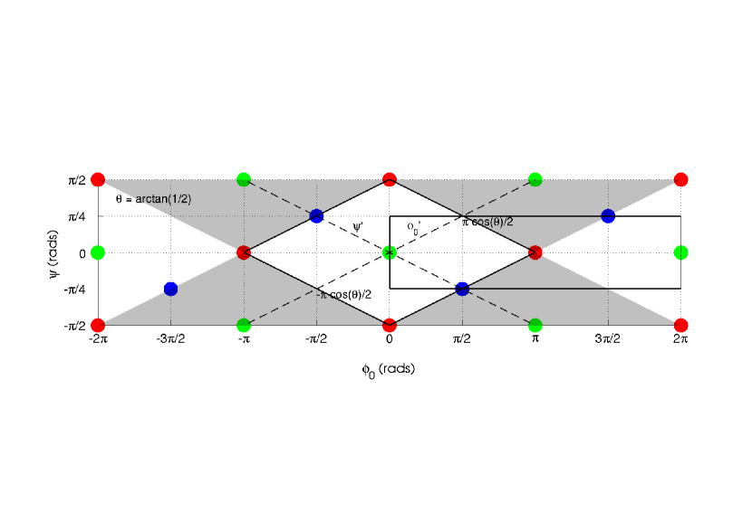
Figure 1: A diagram of the $\phi_{0}$–$\psi$ parameter space demonstrating the new ${\phi^{\prime}}_{0}$–$\psi^{\prime}$ parameterisation. The filled circles represent an area of probability for a signal, with the same colours representing the same signal and showing the degeneracy between parameters. The rectangular box shows the parameters space used in the original code and the diamond box shows the new parameter space.

Given flat priors on $\phi_{0}$ and $\psi$, the above change in variables will mean that the priors on ${\phi^{\prime}}_{0}$ and $\psi^{\prime}$ remain flat (the Jacobian is constant). The new parameters can be converted back to $\phi_{0}$ and $\psi$ via inversion of the transformation matrix giving

$$\phi_{0} ={\phi^{\prime}}_{0}/(2\sin{\theta})-\psi^{\prime}/(2\sin{\theta}),$$

$$\psi ={\phi^{\prime}}_{0}/(2\cos{\theta})+\psi^{\prime}/(2\cos{\theta}).$$ (5)

However, it should be noted that this will return values in the range $-\pi\leq\phi_{0}\leq\pi$ and $-\pi/2\leq\psi\leq\pi/2$, so these have to be appropriately wrapped to cover the standard range.

An example of this new parameterisation on the calculation of a signal’s parameter posteriors can be seen in Figure 2, where a strong fake signal was created at the $\psi$ boundary, with $\phi_{0}=\pi/2$ rads and $\psi=-\pi/4$ rads. It was recovered using the new parameterisation and then converted back into the original parameters correctly, where the bimodality in $\phi_{0}$ can clearly be seen. The MCMC acceptance rate improved from a fraction of a percent to of order 50%. The same result could also be achieved by using this new parameterisation to define a prior volume for $\phi_{0}$ and $\psi$.

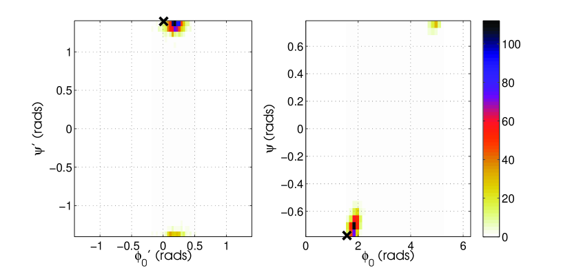
Figure 2: The 2D posterior probability distributions of a fake signal (true parameters marked with the $\times$) extracted with the new ${\phi^{\prime}}_{0}$–$\psi^{\prime}$ parameterisation (left) and converted back into the $\phi_{0}$–$\psi$ parameters (right).

4 Code testing

The old code used in the analyses up to now has been sufficient, but as stated previously has some disadvantages. However, as it is well understood it provides a good check against which to test that the new code is working correctly. We have tested the posterior probability distributions extracted with simulated signals and simulated noise using the new and old codes.

An example is shown in Figure 3, which shows three sets of posterior probability distributions for the four unknown signal parameters of a simulated pulsar signal injected into fake noise from the LIGO Hanford (H1) detector. Two were calculated with the old code in a grid-based mode (with a $50^{4}$ grid over the parameter ranges) and an MCMC mode (with a burn-in of 50 000 points and 100 000 points sampling the posterior) and the third was produced using the new code with the nested sampling algorithm (using a total of 1 250 000 likelihood evaluations). Here we make no assessment of the relative speed/efficiencies of the methods, which mainly depends on the number of likelihood evaluations they each perform, but just test their consistency. As with other injections we have studied all three methods show very good agreement in the posteriors they produce. It should be noted that in setting up the codes the nested sampling code required no tuning, whereas with the old code for the grid-based search and the MCMC the parameter ranges and proposal distributions had to be specified to quite closely match the posterior ranges. All three methods also recover the true signal values within the posteriors.

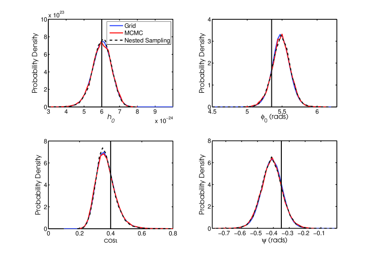
Figure 3: Marginalised posterior probability densities for a fake pulsar signal injected into simulated LIGO Hanford detector noise. The injection parameters are shown as the thin vertical lines. The solid blue lines are the posteriors from the old code with a grid-based approach, the solid red lines are the posteriors from the old code with the basic MCMC approach, and the dashed black lines are from the new code using nested sampling.

4.1 Upper limit testing

Previous astrophysical searches have not seen any signals, so have instead set upper limits on the gravitational wave amplitude, $h_{0}$. Monte Carlo tests have shown the distribution of upper limits (in our case limits at 95% degree-of-belief) that would be expected given many datasets consisting of Gaussian noise of known power spectral density for pulsars randomly distributed on the sky [7]. So, again a good way to test the new code is to check that it can produce the same distribution of upper limits as that found with the old code. Figure 4 shows the distribution of 95% upper limits normalised by the noise power spectral density ($S_{n}$ in Hz^-1) and data length ($T$ in seconds) using the nested sampling code and the old grid-based code.

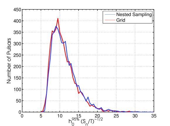
Figure 4: The distribution of 95% degree-of-belief upper limits on $h_{0}$ for 5000 realisations of noise for sources uniformly distributed on the sky using the nested sampling code (blue line) and grid-based code (red line).

These two independent methods are very consistent with each other. The agreement between these distributions and that shown in [7] is good, but not prefect. Without knowing the exact set-up of that earlier analysis we cannot track down the root cause of this discrepancy, but are confident that our current analysis with these two independent methods is correct.

5 Additional models and parameters

The simple 4-dimensional parameter space of the signal given in eq:complexsignal can easily be covered on a grid (although as stated still requires some tuning of grid spacing and parameter ranges). However, there are many cases where the number of parameters in known pulsar searches can greatly increase and model comparisons are required. Here we briefly discuss a couple of cases of this and plans for the future.

5.1 Inclusion of phase parameter uncertainties

As in [5] radio pulsar observations will often come with uncertainties on the parameters, which although in general are very small can mean that the single phase model used in eq:complexsignal is not sufficient to described the signal. These extra parameters describing the phase change need to be incorporated into the gravitational wave search. The new code can incorporate these observed uncertainties, via the phase parameter covariance matrix, to be used as priors. Figure 5 shows the marginalised posteriors for three parameters (frequency, right ascension and declination) that have been estimation from data just containing Gaussian noise, using priors similar to uncertainties from radio observations, with other parameters held fixed. The priors used are also plotted and show that for these phase parameters the posteriors are completely defined by the priors as would be expected for data containing only noise. These priors were also correlated, with the prior correlation coefficients used and correlation coefficients calculated from the posterior given in Table 1. Again these show that the expected prior distribution is being obtained.

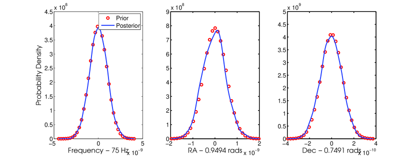
Figure 5: The marginalised posteriors for frequency, right ascension and declination calculated from data consisting of Gaussian noise, using the priors shown.

RA Dec Frequency RA 1.0 0.5 -0.2 Dec 0.5 1.0 -0.7 Frequency -0.2 -0.7 1.0

RA Dec Frequency RA 1.0 0.467 -0.173 Dec 0.467 1.0 -0.694 Frequency -0.173 -0.694 1.0

Table 1: The correlation coefficients of the priors (left) on frequency, right ascension and declination used to produce a posterior (right) for data consisting of Gaussian noise.

There are also potential sources and candidates from all sky searches for unknown pulsars/neutron stars (e.g. [16, 17]) that may have parameters e.g. frequency, frequency derivatives and sky position, with relatively large uncertainties spanning many phase models. The new code has preliminarily been tested in a search search containing a fake signal, with a prior range on the frequency band of $2\times 10^{-3}$ Hz, with the recovered $h_{0}$–frequency posterior shown in Figure 6. The code recovers the injected signal well, but in a future paper we will fully characterise the code for searches over these wider frequency bands, and compare it to similar searches using the $\mathcal{F}$-statistic as applied in [4], or the $\mathcal{B}$-statistic of [9].

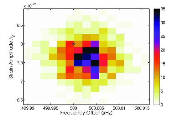
Figure 6: The 2D posterior of signal frequency offset (from the central search frequency) against $h_{0}$ for a fake pulsar signal with a signal-to-noise ratio of $\sim 19$. The true injection parameters are marked with a black cross. The prior volume covered $\pm 10^{-3}$ Hz in frequency offset and 0 to $10^{-22}$ in $h_{0}$.

5.2 Model selection

Nested sampling produces a value of the evidence which can be used for model comparisons. In a future paper the code will be fully characterised for comparing the evidence for the signal model described in Section 1 against a model that the data contains just Gaussian noise. The ratio of these evidences can be used as a detection statistic to assess a candidate signal’s significance. The code is also flexible enough to allow additional models including extra parameters. We plan to assess a new signal model, which can include emission at once and twice the rotation frequency [18] and includes additional angular parameters, and compare it to the standard model given by eq:complexsignal. Further signal and noise models (for example models including interference lines that are incoherent between multiple detectors [19]) could easily be added in the future in the current framework.

6 Conclusions

A new code for parameter estimation and model comparison, based on the nested sampling algorithm, has been developed for continuous-wave searches in gravitational wave data. It has been shown to be consistent with a previous code, used successfully in many searches, in extracting signal parameters and producing upper limits on gravitational wave amplitude. The new code has advantages over the old code in that it requires less tuning for specific searches and allows comparison between different models.

The new code is flexible enough to be expanded to larger numbers of parameters and parameter ranges. This will allow it to be used in searches for pulsars with less well defined parameters, or as a method to follow up candidates from all-sky neutron star searches. These will be characterised in future papers. Additional MCMC proposal distributions for drawing new samples will also be investigated to study improvements in the algorithm’s efficiency. These will including proposals that only update one parameter at a time when drawing from a multivariate Gaussian, using a $k$-D tree of the samples to form a proposal (e.g. [20]) and potentially using MultiNest [21], which has been integrated into the lalinference package of lalsuite [10].

In the near future this code will be used in searches for a large number of known pulsars in data from the recent LIGO S6 and the Virgo VSR2, 3 and 4 data runs.

The authors would like to thank the LIGO Scientific Collaboration and Virgo Collaboration continuous wave and CBC Bayesian parameter estimation working groups, and the developers of the lalinference software suite, for many useful discussions. We also thank the referee for their many useful comments on the draft. The document has LIGO DCC number LIGO-P1100171.

References

References

- [1] Abbott B, Abbott R, Adhikari R, Ageev A, Allen B, Amin R, Anderson S B, Anderson W G, Araya M, Armandula H and et al 2004 Phys. Rev. D 69 082004 (Preprint arXiv:gr-qc/0308050)
- [2] Abbott B, Abbott R, Adhikari R, Ageev A, Allen B, Amin R, Anderson S B, Anderson W G, Araya M, Armandula H and et al 2005 Physical Review Letters 94 181103 (Preprint arXiv:gr-qc/0410007)
- [3] Abbott B, Abbott R, Adhikari R, Agresti J, Ajith P, Allen B, Amin R, Anderson S B, Anderson W G, Arain M and et al 2007 Phys. Rev. D 76 042001 (Preprint arXiv:gr-qc/0702039)
- [4] Abbott B, Abbott R, Adhikari R, Ajith P, Allen B, Allen G, Amin R, Anderson S B, Anderson W G, Arain M A and et al 2008 ApJ 683 L45–L49 (Preprint 0805.4758)
- [5] Abbott B P, Abbott R, Acernese F, Adhikari R, Ajith P, Allen B, Allen G, Alshourbagy M, Amin R S, Anderson S B and et al 2010 ApJ 713 671–685 (Preprint 0909.3583)
- [6] Abadie J, Abbott B P, Abbott R, Abernathy M, Accadia T, Acernese F, Adams C, Adhikari R, Affeldt C, Allen B and et al 2011 ApJ 737 93 (Preprint 1104.2712)
- [7] Dupuis R J and Woan G 2005 Phys. Rev. D 72 102002 (Preprint arXiv:gr-qc/0508096)
- [8] Weinberg M D 2009 ArXiv e-prints (Preprint 0911.1777)
- [9] Prix R and Krishnan B 2009 Classical and Quantum Gravity 26 204013 (Preprint 0907.2569)
- [10] URL https://www.lsc-group.phys.uwm.edu/daswg/projects/lalsuite.html
- [11] van der Sluys M, Raymond V, Mandel I, Röver C, Christensen N, Kalogera V, Meyer R and Vecchio A 2008 Classical and Quantum Gravity 25 184011 (Preprint 0805.1689)
- [12] Röver C, Meyer R and Christensen N 2007 Phys. Rev. D 75 062004 (Preprint arXiv:gr-qc/0609131)
- [13] Veitch J and Vecchio A 2010 Phys. Rev. D 81 062003 (Preprint 0911.3820)
- [14] Skilling J 2006 Bayesian Analysis 1 833–860
- [15] Sivia D S and Skilling J 2006 Data Analysis: A Bayesian Tutorial (Oxford University Press) chap 9
- [16] Abbott B P, Abbott R, Adhikari R, Ajith P, Allen B, Allen G, Amin R S, Anderson S B, Anderson W G, Arain M A and et al 2009 Phys. Rev. D 80 042003 (Preprint 0905.1705)
- [17] Abadie J, Abbott B P, Abbott R, Abbott T D, Abernathy M, Accadia T, Acernese F, Adams C, Adhikari R, Affeldt C and et al 2011 ArXiv e-prints (Preprint 1110.0208)
- [18] Jones D I 2010 MNRAS 402 2503–2519 (Preprint 0909.4035)
- [19] Keitel D, Prix R, Alessandra Papa M and Siddiqi M 2012 ArXiv e-prints (Preprint 1201.5244)
- [20] Farr W M and Mandel I 2011 ArXiv e-prints (Preprint 1104.0984)
- [21] Feroz F, Hobson M P and Bridges M 2009 MNRAS 398 1601–1614 (Preprint 0809.3437)