Statistical Characterization and Mitigation of NLOS Bias in UWB Localization Systems

Abstract

In this paper the problem of the joint statistical characterization of the NLOS bias and of the most representative features of LOS/NLOS UWB waveforms is investigated. In addition, the performance of various maximum-likelihood (ML) estimators for joint localization and NLOS bias mitigation is assessed. Our numerical results evidence that: a) the accuracy of all the considered estimators is appreciably affected by the LOS/NLOS conditions of the propagation environment; b) a statistical knowledge of multiple signal features can be exploited to mitigate the NLOS bias, so reducing the overall localization error.

I Introduction

Wireless localization in harsh communication environments (e.g., in a building where wireless nodes are separated by concrete walls and other obstacles) can be appreciably affected by direct path attenuation and NLOS conditions. In principle, the effects of NLOS errors can be mitigated adopting techniques for detecting LOS/NLOS conditions or algorithms for estimating the errors themselves (i.e., the bias due to obstacles). These approaches can potentially improve the overall accuracy and are expected to satisfy certain requirements; in particular, they should be robust against changes in the propagation environment, stable (i.e., they should never amplify NLOS errors) and should be able to exploit all the available data (e.g., received waveforms and a priori information).

Various solutions for NLOS error mitigation in UWB environments are available in the technical literature [1], [2], [3], [4]. In particular, a simple deterministic model, dubbed wall extra delay, is proposed in [1] to estimate the bias introduced by walls. A non-parametric support vector machine is employed in [2] for joint bias mitigation and channel status detection; this approach exploits multiple features extracted from received signals in a non-statistical fashion. A few classification algorithms for LOS/NLOS detection are compared in [3], where it is shown that the best solution is offered by a statistical strategy based on the joint probability density function (pdf) of the delay spread and the kurtosis extracted from the received signals. Finally, in [4] statistical models for the time of arrival (TOA), the received signal strength (RSS) and the root mean square delay spread (RDS) are developed and an iterative estimator for bias mitigation is devised.

The contribution of this paper is twofold. In fact, first of all, the problem of joint statistical modeling of multiple features extracted from a database of waveforms acquired in a TOA-based localization system is investigated. Note that, as far as we know, in the technical literature only univariate models for bias mitigation have been proposed until now (e.g., see [1], [4] and [5]). The use of multiple signal features in UWB localization systems has been investigated in [3] for channel state detection only and in [6], where, however, the considered features (namely, the kurtosis, the mean excess delay and the delay spread) have been modelled as independent random variables. The second contribution offered by this manuscript is represented by a performance comparison of various maximum-likelihood (ML) estimators for TOA-based localization. In particular, unlike other papers (e.g., see [2], [3]) we illustrate some numerical results referring to the accuracy of different localization strategies, rather than to capability of the bias removal on a single radio link.

The remaining part of this paper is organized as follows. In Section II some information about our UWB experimental campaign and about the features extracted from the acquired data are provided. In Section III some estimation algorithms for UWB radiolocalization are described, whereas their performance is compared in Section IV. Finally, some conclusions are given in Section V.

II Experimental setup

II-A Measurement arrangement

A measurement campaign was conducted by our research group in the second half of 2010 in order to assess the impact of NLOS bias errors on a real world UWB system for localization; all the measured data were acquired by means of two FCC-compliant PulsON220 radios commercialised by TimeDomain and were collected in a database. Such devices are equipped with omnidirectional antennas, are characterized by a -10 dB bandwidth and a central frequency equal to 3.2 GHz and 4.7 GHz, respectively, and perform two-way TOA ranging; they also allow to store digitised received waveforms (a sampling frequency of 24.2 GHz and 14 bits per sample are used).

It is worth mentioning that various databases providing a collection of sampled UWB waveforms acquired in experimental campaigns and useful for assessing the performance of localization algorithms are already available (e.g., see [7], [8]). However, our database has been specifically generated to assess the correlation between the NLOS bias error and various features extracted from the received signals, as it will become clearer in the next Paragraph. Our measurement campaign consisted of two phases. First, the transmitter was placed in a given room (room A in Fig. 1) and the receiver in an adjacent room (room B in Fig. 1) separated from room A by a wall having thickness $t_{wall}=32$ cm (NLOS condition); in addition, the transmit antenna was kept fixed, whereas the receive antenna was placed in $N_{acq}^{\text{\tiny{NLOS}}}=174$ distinct vertices of a dense square grid (the distance between a couple of nearest vertices was equal to 21 cm). In the second phase of our measurement campaign both the transmitter and the receiver were placed in room B; then, the transmit antenna was kept fixed, whereas the receive antenna was moved on the same dense grid as in the first phase to acquire the UWB waveform in $N_{acq}^{\text{\tiny{LOS}}}=105$ distinct vertices. The positions of the transmit antenna in the two phases were $(0.26,2.97)$ m and $(0.26,3.97)$ m, respectively, if the coordinate system shown in Fig. 1 is employed. The distance between the two antennas varied between 1 m and about 5 m; larger distances were not taken into consideration since we were interested in indoor ranging only. It is important that to note that the choice of the measurement scenarios described above is motivated by the fact that UWB signals experienced similar propagation in both phases.

For each position of the receive antenna up to 25 realizations of the received UWB signal were acquired (each one lasting $T_{acq}=110$ ns), in order to filter out the effects of the measurement noise and the TOA estimate outliers in the postprocessing phase. The analysis of the multiple waveforms referring to each link evidenced the presence of few time-variant artifacts (mostly due to the movements of the people behind the radios); as a matter of fact, the channel in our measurement campaign can be deemed quasi-static and is characterized by reflections mainly due to the walls, the ceiling and the floor of the room (or rooms) hosting the radio devices.

Finally, for each acquired waveform, a TOA estimate (evaluated by the PulsON220 devices) and the actual transmitter-receiver distance (evaluated by means of a metric tape with an accuracy better than 1 cm) were also stored in the database. The TOA estimates have been used to provide a common time frame to all the acquired waveforms; this has made possible the estimation of the mean excess delay and of other signal statistics in the signal processing phase.

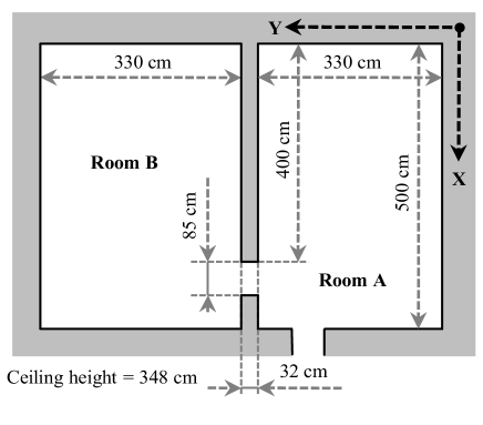
Figure 1: Map of the enviroment of our experimental campaign.

II-B Statistical modeling of signal features

In each of the two measurement phases described in the previous Paragraph, the procedure for acquiring UWB waveforms worked as follows. First, the UWB radios carried out their handshaking procedure for achieving mutual time synchronization; then, the receiver sampled the incoming waveforms and generated a TOA estimate for each of them; let $r_{i}^{\text{\tiny{LOS}}}(t)$ ($r_{i}^{\text{\tiny{NLOS}}}(t)$) and $\tau_{i}^{\text{\tiny{LOS}}}\triangleq\mathrm{TOA}(r_{i}^{\text{\tiny{LOS}}}(t))$ ($\tau_{i}^{\text{\tiny{NLOS}}}\triangleq\mathrm{TOA}(r_{i}^{\text{\tiny{NLOS}}}(t))$) denote the received waveform and the corresponding TOA estimate (here the function $\mathrm{TOA}(\cdot)$ represents the internal procedure adopted by the PulsON220 devices, based on energy thresholds and a go-back technique, to estimate the TOA; see [9] for further details) acquired over the $i$-th link in LOS (NLOS) conditions. The model

$$\tau_{i}=\frac{d_{i}}{c_{0}}+b_{i}+w_{i}$$ (1)

was adopted for the measured TOA (for both LOS and NLOS conditions). Here, $c_{0}$ is the speed of light, $d_{i}$ denotes the distance between the transmitter and the receiver, $b_{i}$ is the NLOS bias (in seconds) affecting the TOA measurement (the values taken on by this random parameter are always positive for NLOS links and null for LOS links) and $w_{i}\sim\mathcal{N}(0,\sigma_{w,i}^{2})$ is the measurement noise; in addition, the expression $\sigma_{w,i}^{2}=\gamma\sigma_{n}^{2}d_{i}^{\beta}$ is adopted for the variance of the measurement noise, where $\gamma$ is a parameter depending on both the specific TOA estimator employed in the ranging measurements and on various parameters of the physical layer, and $\beta$ is the path-loss exponent (a known and fixed value is assumed for this parameter in both LOS and NLOS conditions [4]).

Correlation with $b_{i}$	$x_{i,0}$	$x_{i,1}$	$x_{i,2}$	$x_{i,3}$	$x_{i,4}$	$x_{i,5}$	$d_{i}$
NLOS case	0.795	0.852	0.894	0.641	0.454	0.644	0.609
LOS case	0.602	0.586	0.129	0.666	0.586	0.119	0.629

Table I: Absolute values of correlation coefficients between $b_{i}$ and $x_{i,j}$, with $j=0,....,N_{f}-1$.

In the following we focus on the problem of estimating the bias $b_{i}$ (affecting the TOA estimate $\tau_{i}$ (1)) from a set of $N_{f}=6$ different “features” $\left\{x_{i,j}\text{, }j=0\text{, }1\text{, }...\text{, }5\right\}$ extracted from the received waveform $r_{i}(t)$. In particular, like in [2], the following features were evaluated for the set of the received waveforms:

1. the maximum signal amplitude $x_{i,0}=r_{max,i}\triangleq\max_{t}|r_{i}(t)|$;

2. the mean excess delay $x_{i,1}=\tau_{m,i}\triangleq\int_{0}^{\infty}t\frac{|r_{i}(t)|^{2}}{\varepsilon_{i}}dt$ (the parameter $\varepsilon_{i}$ is defined below);

3. the delay spread $x_{i,2}=\tau_{ds,i}\triangleq\int_{0}^{\infty}(t-\tau_{m,i})^{2}\frac{|r_{i}(t)|^{2}}{\varepsilon_{i}}dt$;

4. the energy $x_{i,3}=\varepsilon_{i}\triangleq\int_{0}^{\infty}|r_{i}(t)|^{2}dt$;

5. the rise time $x_{i,4}=t_{rise,i}\triangleq\min\left\{t:|r_{i}(t)|/\max_{t}|r_{i}(t)|>0.9\right\}-\min$ $\left\{t:|r_{i}(t)|/\max_{t}|r_{i}(t)|>0.1\right\}$;

6. the kurtosis $x_{i,5}=\kappa_{i}\triangleq\frac{1}{\sigma_{|r|}^{4}T}\int_{T}\left(|r_{i}(t)|-\mu_{|r|}\right)^{4}dt$, where $\mu_{|r|}\triangleq\frac{1}{T}$ $\int_{T}|r_{i}(t)|dt$, $\sigma_{|r|}^{2}\triangleq\frac{1}{T}\int_{T}(|r_{i}(t)|-\mu_{|r|})^{2}dt$ and $T$ denotes the observation time.

In the following the set $\left\{r_{i}(t)\right\}$ of received waveforms is modelled as a random process, so that the above mentioned features form a set of correlated random variables; in addition, all of them are statistically correlated with the TOA bias. The last consideration is confirmed by the numerical results of Table I, which lists the absolute values of the correlation coefficients of the previously described features with the estimated TOA bias for both the LOS and the NLOS scenarios. From these results it can be easily inferred that not all the considered features are equally useful to estimate the TOA bias. For this reason and to simplify our statistical analysis, we restricted the group of considered features to the set $\{x_{i,0}$, $x_{i,1}$, $x_{i,2}\}$, which collects the parameters exhibiting a strong correlation with the bias in the NLOS scenario.

Note that, in principle, the bias $b_{i}$ is not influenced by the distance $d_{i}$, since it depends only on the thickness of the walls (or of other obstacles) encountered by the transmitted signal during its propagation; this is not true, however, for the above mentioned triple of signal features (see [1] for further details). Generally speaking, it is useful to derive a TOA bias estimator which is not influenced by the transmitter-receiver distance $d_{i}$. In the attempt of removing the dependence of the features $\{x_{i,0}$, $x_{i,1}$, $x_{i,2}\}$ on the link distance, we developed the models

$$x_{i,0}=r_{max,i}=r_{max}^{0}-r_{max}^{m}d_{i}\text{,}$$ (2)

$$x_{i,1}=\tau_{m,i}=\tau_{m}^{m}d_{i}$$ (3)

and

$$x_{i,2}=\tau_{ds,i}=\tau_{ds}^{0}+\tau_{ds}^{m}d_{i}$$ (4)

on the basis of our experimental results (and, in particular, on the basis of the estimates of the joint pdf’s $\{f_{b,x_{0}}$, $f_{b,x_{1}}$, $f_{b,x_{2}}\}$ referring to the three possible couples $(b_{i}$, $x_{i,j})$ with $j=0$, $1$, $2$); here $r_{max}^{0}$, $\tau_{m}^{m}$ and $\tau_{ds}^{m}$ are random variables, whereas $\tau_{ds}^{0}$ and $r_{max}^{m}$ are deterministic parameters having known values. Given these models, the vector of distance-independent features $\tilde{\mathbf{x}}\triangleq\left[r_{max}^{0},\tau_{m}^{m},\tau_{ds}^{m}\right]^{T}$ can be evaluated from its distance-dependent counterpart $\mathbf{x}=\left[r_{max},\tau_{m},\tau_{ds}\right]^{T}$and can be used in place of it.

A complete statistical characterization of the estimated bias and of the $3$ related signal features we consider is provided by the joint pdf $f_{b,r_{max},\tau_{m},\tau_{ds}}(\cdot)$ or, equivalently, by the joint pdf $f_{b,r_{max}^{0},\tau_{m}^{m},\tau_{ds}^{m}}(\cdot)$; these functions have been estimated from the acquired data, but cannot be plotted because of the large dimensionality of their domains; for this reason, we analysed some pdf’s deriving from their marginalization. For instance, Fig. 2 shows the estimated joint pdf’s for the estimated bias $\hat{b}_{i}$ and measured delay spread for the NLOS and the LOS scenarios; these results deserve the following comments:

1. a significant (limited) correlation between these parameters is found in the NLOS (LOS) case;

2. the null region exhibited by the estimated pdf’s is due to the fact that the TOA bias cannot take on values in the interval $[0,\>t_{wall}/c_{0}]$, where $t_{wall}$ is the thickness of the wall obstructing the direct path;

3. large values of the TOA bias are unlikely since they are associated with small incidence angles of the transmitted signal on the obstructing wall.

   

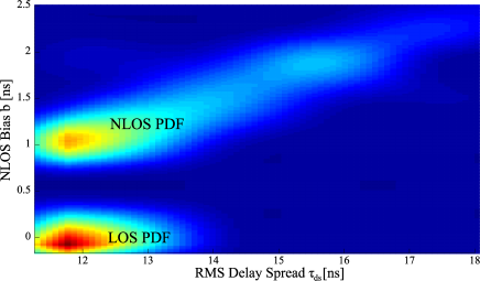
   Figure 2: Estimated joint pdf of the estimated TOA bias and the delay spread in NLOS conditions (above) and LOS conditions (below). Note that the NLOS PDF has been scaled by a factor 3 to improve its visualization.

   

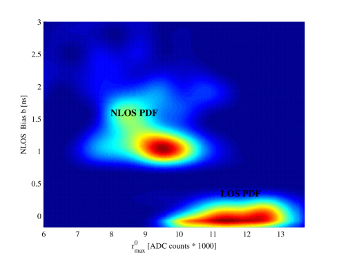
   Figure 3: Estimated joint pdf of the estimated TOA bias and the $r_{max}^{0}$ random variable in NLOS conditions (above) and LOS conditions (below). Note that the NLOS PDF has been scaled by a factor 2 to improve its visualization.

Finally, it is important to point out that our experimental data were also processed to evaluate the correlation coefficient between the estimated bias $\hat{b}_{i}$ and each of the distance-independent parameters $r_{max}^{0}$, $\tau_{m}^{m}$ and $\tau_{ds}^{m}$ (see Table II and Fig. 3, which represents the joint pdf of the estimated bias $\hat{b}_{i}$ and the parameter $r_{max}^{0}$); our results evidence that the last parameters are less correlated with $b_{i}$ than their distance dependent counterparts. For this reason, we decided to take into consideration also the distance-dependent features $\{x_{i,0}$, $x_{i,1}$, $x_{i,2}\}$ for localization purposes.

Correlation with $b_{i}$	$\tilde{x}{}_{i,0}$ $r_{max,i}^{0}$	$\tilde{x}{}_{i,1}$ $\tau_{m,i}^{m}$	$\tilde{x}{}_{i,2}$ $\tau_{ds,i}^{m}$
NLOS case	0.321	0.649	0.561
LOS case	0.483	0.370	0.490

Table II: Absolute values of correlation coefficients between the estimated bias $\hat{b}_{i}$ and each of the parameters $r_{max}^{0}$, $\tau_{m}^{m}$ and $\tau_{ds}^{m}$. Both LOS and NLOS conditions are considered.

III Localization algorithms

III-A Introduction

In this Section we develop various algorithms for two-dimensional localization in a UWB network composed by $N_{a}$ anchors with known positions $\mathbf{z}_{i}^{a}\triangleq\left[x_{i}^{a},\,y_{i}^{a}\right]^{T}\in\mathbb{R}^{2}$, $i=0,...,N_{a}-1$ and by a single node (dubbed mobile station, MS, in the following) with unknown position $\boldsymbol{\theta}\triangleq[x,\,y]^{T}\in\mathbb{R}^{2}$. Any couple of the given $(N_{a}+1)$ devices can operate in a LOS (NLOS) condition with probability $P_{\text{\tiny{LOS}}}$ ($1-P_{\text{\tiny{LOS}}}$). The localization algorithms described below try to mitigate the effects of the NLOS bias error and aim at generating an estimate $\hat{\boldsymbol{\theta}}$ of $\boldsymbol{\theta}$ minimizing the mean square error (MSE) $\mathbb{E}_{\mathbf{\hat{\boldsymbol{\theta}}}}\left\{||\mathbf{\hat{\boldsymbol{\theta}}}-\mathbf{\boldsymbol{\theta}||}^{2}\right\}$. It is also important to point out that localization algorithms developed for NLOS scenarios usually consist of two steps. In fact, first the NLOS bias is estimated for each involved link and is used to remove the bias contribution in the acquired data; then the new data set is processed by a least-square (LS) procedure generating an estimate of $\mathbf{\boldsymbol{\theta}}$ (e.g., see [2], [3], [4], [6]). A different approach, involving implicit estimation of the bias for each link, is adopted in the following; this approach is motivated by the fact that the estimation of the bias for the $i$-th link can benefit from the information acquired from the other ($N_{a}-1$) links; note that in [2] and [6] bias mitigation performed in a link-by-link fashion is exploited to assign a weight in a weighted least-square (WLS) step, but such an approach is heuristic.

III-B Maximum Likelihood Estimation

If the links between the MS and the $N_{a}$ different anchors are assumed mutually independent, the ML estimation strategy of the unknown MS position $\mathbf{\boldsymbol{\theta}}$, given a TOA estimate and a set of additional signal features for each link, can be formulated as

$$\mathbf{\hat{\boldsymbol{\theta}}}=\arg\underset{\mathbf{\tilde{\boldsymbol{\theta}}}}{\max}\ln\prod_{i=0}^{N_{a}-1}f_{\mathbf{\tau},\mathbf{x}}(\tau_{i},\mathbf{x}_{i};\mathbf{\tilde{\boldsymbol{\theta}}})\text{.}$$ (5)

Here, $\mathbf{\tilde{\boldsymbol{\theta}}}=[\tilde{x},\,\tilde{y}]^{T}\in\mathbb{R}^{2}$ denotes the MS trial position, $\tau_{i}$ and $\mathbf{x}_{i}$ are the TOA and $N_{f}$-dimensional signal vector collecting the received signal features acquired for the $i$-th link and $f_{\tau,\mathbf{x}}(\cdot,\mathbf{\cdot};\mathbf{\tilde{\boldsymbol{\theta}}})$ is the joint pdf of the TOA and the vector of features parameterized by the trial position $\mathbf{\tilde{\boldsymbol{\theta}}}$. As already discussed in Paragraph II-B, various options for $\mathbf{x}$ (and, consequently, for $f_{\tau,\mathbf{x}}(\cdot,\mathbf{\cdot};\mathbf{\tilde{\boldsymbol{\theta}}})$) are possible; in the following Paragraphs the impact of such options on the ML strategy (5) is investigated.

III-B1 ML estimation strategy for different sets of observed data

In this Paragraph two different options are considered for the set of features processed by the ML strategy.

Option A

In this case it is assumed that the vector of features referring to the $i$-th link is $\mathbf{x}_{i}=[r_{max,i},\tau_{m,i},\tau_{ds,i}]^{T}$; this choice is motivated by the large correlation between these random variables and the link bias $b$ (see Paragraph II-B). Then, the joint PDF $f_{\mathbf{\tau},\mathbf{x}}(\tau_{i},\mathbf{x}_{i};\mathbf{\tilde{\boldsymbol{\theta}}})$ appearing in the ML strategy (5) can be expressed as (see Eq. (1)):

$$f_{\tau,\mathbf{x}}(\tau_{i},\mathbf{x}_{i};\tilde{\boldsymbol{\theta}})=(f_{b,\tilde{\mathbf{x}}}\otimes f_{w})\left(\tau_{i}-\frac{d_{i}(\mathbf{\tilde{\boldsymbol{\theta}}})}{c_{0}},\tilde{\mathbf{x}}_{i}\right),$$ (6)

where (see Eq. (2), (3), (4))

$$\tilde{\mathbf{x}}_{i}=\left[r_{max,i}+r_{max}^{m}d_{i}(\mathbf{\tilde{\boldsymbol{\theta}}}),\frac{\tau_{m,i}}{d_{i}(\mathbf{\tilde{\boldsymbol{\theta}}})},\frac{\tau_{ds,i}-\tau_{ds}^{0}}{d_{i}(\mathbf{\tilde{\boldsymbol{\theta}}})}\right]^{T}$$ (7)

$d_{i}(\mathbf{\tilde{\boldsymbol{\theta}}})$ is the distance between the $i$-th anchor and the MS trial position and $f_{b,\tilde{\mathbf{x}}}\otimes f_{w}$ denotes the convolution between the joint pdf $f_{b,\tilde{\mathbf{x}}}(\cdot)$ and the observation noise pdf $f_{w}(w)=(2\pi\sigma_{w}^{2})^{-1/2}\exp(-w^{2}/(2\sigma_{w}^{2}))$.

Note that the shape of the function $f_{b,\tilde{\mathbf{x}}}(\cdot)$ under the hypothesis of LOS conditions ($H_{\text{\tiny{LOS}}}$ event) is substantially different from that found in NLOS conditions ($H_{\text{\tiny{NLOS}}}$ event) [4]; in both cases this function was estimated applying the procedure described in [1] to the data collected in our measurement campaign. This led to two distinct multidimensional histograms, which approximate the required pdf’s $f_{b,\tilde{\mathbf{x}}}\left(b,\tilde{\mathbf{x}}_{i}|H_{\text{\tiny{LOS}}}\right)$ and $f_{b,\tilde{\mathbf{x}}}\left(b,\tilde{\mathbf{x}}_{i}|H_{\text{\tiny{NLOS}}}\right)$ with a certain accuracy depending on: a) the amount of acquired data; b) the sizes $\Delta b$, $\Delta r_{max}$, $\Delta\tau_{m}$ and $\Delta\tau_{ds}$ of the quantization bins adopted in the generation of the histograms. Note that these sizes need to be accurately selected, since large bins imply a coarse approximation of pdf’s, whereas excessively small bins require a huge amount of data.

Given an estimate of the above mentioned couple of pdf’s, the pdf $f_{b,\tilde{\mathbf{x}}}(\cdot)$ can be evaluated as

$$f_{b,\tilde{\mathbf{x}}}\left(b,\tilde{\mathbf{x}}_{i}\right) = P_{\text{\tiny{LOS}}}f_{b,\tilde{\mathbf{x}}}\left(b,\tilde{\mathbf{x}}_{i}|H_{\text{\tiny{LOS}}}\right)+$$ (8)

$$\left(1-P_{\text{\tiny{LOS}}}\right)f_{b,\tilde{\mathbf{x}}}\left(b,\tilde{\mathbf{x}}_{i}|H_{\text{\tiny{NLOS}}}\right)$$

if the probabilities $P_{\text{\tiny{LOS}}}\triangleq\Pr\{H_{\text{\tiny{LOS}}}\}$ and $P_{\text{\tiny{NLOS}}}\triangleq\Pr\{H_{\text{\tiny{NLOS}}}\}=1-\Pr\{H_{\text{\tiny{LOS}}}\}$ are available, or as

$$f_{b,\tilde{\mathbf{x}}}\left(b,\tilde{\mathbf{x}}_{i}\right)=\frac{1}{2}f_{b,\tilde{\mathbf{x}}}\left(b,\tilde{\mathbf{x}}_{i}|H_{\text{\tiny{LOS}}}\right)+\frac{1}{2}f_{b,\tilde{\mathbf{x}}}\left(b,\tilde{\mathbf{x}}_{i}|H_{\text{\tiny{NLOS}}}\right)$$ (9)

if no a priori information about the LOS/NLOS conditions are available.

In principle, evaluating the joint PDF $f_{\mathbf{\tau},\mathbf{x}}(\tau_{i},\mathbf{x}_{i};\mathbf{\tilde{\boldsymbol{\theta}}})$ of the ML strategy entails the computation of the convolution appearing in (6); this has not been done in our work, since it is numerically complicated and a form of implicit smoothing is already included in the generation of the above mentioned histograms extracted from the available measurements.

Option B

In this case the set of features employed in ML estimation consists of a single element, namely the delay spread (which exhibits the largest correlation with the NLOS bias; see Table I), so that $\mathbf{x}_{i}=\tau_{ds,i}$ and the pdf $f_{\mathbf{\tau},\mathbf{x}}(\tau_{i},\mathbf{x}_{i};\mathbf{\tilde{\boldsymbol{\theta}}})$ of (5) becomes (see (6))

$$f_{\tau,\mathbf{x}}(\tau_{i},\mathbf{x}_{i};\tilde{\boldsymbol{\theta}})=(f_{b,\tau_{ds}^{m}}\otimes f_{w})\left(\tau_{i}-\frac{d_{i}(\mathbf{\tilde{\boldsymbol{\theta}}})}{c_{0}},\frac{\tau_{ds,i}-\tau_{ds}^{0}}{d_{i}(\mathbf{\tilde{\boldsymbol{\theta}}})}\right)$$ (10)

Like in the previous case, the pdf $f_{b,\tau_{ds}^{m}}(\cdot)$ was estimated in the LOS and NLOS scenarios (see Fig. 2) from the data acquired in our measurement campaign. Note that this option leads to a ML localization algorithm which is substantially simpler than that proposed in the analysis of option A.

III-B2 Parameterization of the observations

The ML strategies developed above are based on the joint pdf’s $f_{b,r_{max}^{0},\tau_{m}^{m},\tau_{ds}^{m}}(\cdot)$ and $f_{b,\tau_{ds}^{m}}(\cdot)$, which refer to a set of distance-independent parameters. Since the parameters $r_{max}^{0}$, $\tau_{m}^{m}$ and $\tau_{ds}^{m}$ exhibit a lower correlation with $b$ than their distance-dependent counterparts $r_{max}$, $\tau_{m}$, $\tau_{ds}$ (see Tables I and II), the use of the joint PDF

$$f_{\tau,\mathbf{x}}(\tau_{i},\mathbf{x}_{i};\mathbf{\tilde{\boldsymbol{\theta}}})=(f_{b,\mathbf{x}}\otimes f_{w})\left(\tau_{i}-\frac{d_{i}(\tilde{\boldsymbol{\theta}})}{c_{0}},\mathbf{x}_{i}\right)$$ (11)

in place of (6) has been also investigated (similar comments apply to (10)).

III-B3 Estimation of joint pdf’s

As already explained above, the joint pdf’s involved in the proposed ML localization strategies can be easily estimated from the acquired data using a simple procedure based on dividing the space of observed data in a set of bins of proper size. Such a procedure generates an histogram, which, unluckily, entails poor localization performance if employed as it is, because of the relatively small number of bins (adopted to avoid empty bins). To mitigate this problem, interpolation followed by low-pass filtering can be applied to raw experimental histograms. In particular, we found out that cubic spline interpolation followed by moving average filtering (with a window size equal to about 1/15 of the size of the histogram) provides good results (an example of the resulting pdf is shown in Fig. 2); the localization strategies adopting this approach are dubbed interpolated-histogram estimators in the following.

An alternative to this approach is represented by fitting the histograms with analytical functions (e.g., polynomials). On the one hand, this solution offers some advantages with respect to the previous one, since it requires less memory (only the values of the coefficients of the fitting equations need to be saved) and provides better accuracy (the resulting pdf’s are smoother). On the other hand, the use of (multi-dimensional) fitting raises a number of problems. In fact, global performance figures, like the root mean square error (RMSE) are certainly useful, but do not account for the fact that fitting errors where a pdf takes on small values are less critical than those in points where the same pdf takes on large values. In addition, if the dimensionality of the pdf domain is larger than two, an analytical function generated by a fitting procedure cannot be easily represented.

In our statistical analysis, the use of polynomial fitting was investigated. A polynomial degree $N_{pol}=8$ was selected, since this choice ensures that the resulting RMSE is smaller than $\epsilon_{fitting}=5\cdot 10^{-4}$ in both LOS and NLOS scenarios. In the following localization algorithms employing pdf’s generated by polynomial fitting will be dubbed fitted-histogram estimators.

III-C Iterative Estimation

Recently, an iterative estimator of both the channel state (i.e., LOS or NLOS conditions) and the NLOS bias $b$ has been proposed in [4]. Such an estimator relies on the availability of univariate statistical models for the estimates of TOA, RSS and RDS; it is shown, however, that estimation accuracy is improved if the delay-spread is exploited as the only discriminant feature.

In the following, a modified version of this iterative algorithm (dubbed iterative estimator), employing the joint pdf’s described above and extracted from our experimental database, is proposed. This algorithm is summarized by the flow diagram shown in Fig. 4 and operates as follows. In its first iteration it starts with a null estimate of the NLOS bias and, for each link, generates a set of posterior probabilities integrating the pdf’s estimated in LOS and NLOS conditions. Then, such probabilities are employed to compute a couple of decision variables on the basis of which a decision $\hat{H}$ on the LOS/NLOS conditions is taken. Finally, such a decision is exploited to compute a new bias estimate which is used to start the next iteration. Note that this algorithm operates in a link-by-link fashion and that in the diagram of Fig. 4 the dependence on the link index has been omitted to ease the reading.

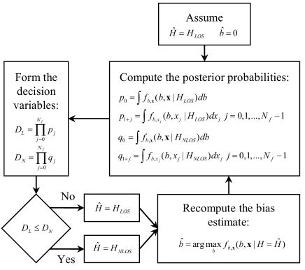
Figure 4: Flow diagram of the proposed iterative estimator.

IV Numerical results

Our experimental database has also been exploited to assess the RMSE performance of the proposed algorithms for localization and NLOS bias mitigation schemes via computer simulations. In our simulations the MS coordinates are always $(0;0)$; then, following [2], for the $i$-th anchor a received waveform from either the LOS database (with probability $P_{\text{\tiny{LOS}}}$) or from the NLOS database (with probability $P_{\text{\tiny{NLOS}}}$) was drawn randomly and was associated with the position $\mathbf{z}_{i}^{a}=\left(d_{i}\sin(2\pi\frac{i-1}{N_{a}});d_{i}\cos(2\pi\frac{i-1}{N_{a}})\right)$, where $d_{i}$ is the distance measured for the selected waveform. Note that these waveforms already include the experimental noise and thus no simulated noise was imposed on the waveforms (so that the signal-to-noise ratio is the experimental one). Finally, the parameter $N_{a}$ has been set to $3$ (worst case which still theoretically allows unambiguous localization).

The RMSE performance of the following algorithms has been evaluated:

1. LS - A standard LS estimator for LOS environments; the estimation strategy can be expressed as $\hat{\mathbf{\boldsymbol{\theta}}}=\arg\min_{\mathbf{\tilde{\boldsymbol{\theta}}}}\sum_{i=0}^{N_{a}-1}(c_{0}\tau_{i}-d_{i}(\mathbf{\tilde{\boldsymbol{\theta}}}))^{2}$.

2. VE - A LS estimator exploiting TOA measurements corrected by the algorithm proposed by Venkatesh and Buehrer in [4]; this algorithm relies on a statistical modeling of the propagation environment based on our experimental database.

3. ML-4D - A ML estimator based on (9) and employing an interpolated histogram for the evaluation of its likelihood function referring to a distance-dependent parameterization.

4. ML-2D - A ML estimator based on (10) and employing an interpolated histogram for the evaluation of its likelihood function referring to a distance-dependent parameterization.

5. ML-2D-ID - A ML estimator based on (10) and employing an interpolated histogram for the evaluation of its likelihood function referring to a distance-independent parameterization.

6. ML-4D-F - A ML estimator based on (9) and employing a fitted histogram for the evaluation of its likelihood function referring to a distance-dependent parameterization.

7. ML-4D-IT - A LS estimator based on (9) and exploiting TOA measurements corrected by the modified iterative algorithm illustrated in Section III-C.

8. ML-2D-IT - A LS estimator based on (10) and exploiting TOA measurements corrected by the modified iterative algorithm illustrated in Section III-C.

In estimating the RMSE performance of the ML algorithms listed above the likelihood functions were always evaluated at the vertices of a square grid characterized by a step size equal to $10$ mm. Some numerical results are compared in Fig. 5, which illustrates the RMSE performance versus the probability $P_{\text{\tiny{LOS}}}$. These results evidence that:

1. Different estimators can provide significantly different accuracies for distinct values of $P_{\text{\tiny{LOS}}}$, when this probability is not close to unity.

2. The simple LS algorithm is outperformed by all the other algorithms when $P_{\text{\tiny{LOS}}}\leq 0.9$; this is due to the fact that this strategy does not try to mitigate the NLOS bias.

3. The VE algorithm performs well at the cost of a reasonable complexity, but offers limited bias mitigation when $P_{\text{\tiny{LOS}}}=0$; in this case the ML-2D, ML-2D-ID and ML-4D-F estimators perform much better.

4. The exploitation of a large set of received signal features does not necessarily allow to achieve better accuracy than a subset of them (see the curves referring to ML-2D and ML-4D estimators); this is due to the fact that the correlation between the different couples of extracted features is typically large, so that they provide strongly correlated information about the NLOS bias.

5. Distance-dependent parameterization provides better accuracy (see the curves referring to the ML-2D and ML-2D-ID estimators); this can be related to the fact that $\tau_{ds}^{m}$ is less correlated with the NLOS bias than its distance-dependent counterpart $\tau_{ds}$.

6. The ML-4D-F estimator performs better than the ML-4D estimator in NLOS conditions; this means that the use of fitted histograms entails an improvement in localization accuracy.

Finally, Fig. 6 shows the cumulative density function (CDF) of the RMSE localization error characterizing the LS, VE, ML-2D and ML-2D-IT algorithms when $P_{\text{\tiny{LOS}}}=0.2$. These results evidence that: a) the RMSE localization error of the considered algorithms remains below $0.5$ m in average the 80% of the cases; b) the ML-2D technique is more accurate than the other algorithms, in terms of RMSE, for small NLOS errors.

Figure 5: RMSE performance versus $P_{\text{\tiny{LOS}}}$ offered by various localization algorithms.

Figure 6: CDFs of the RMSE characterizing various localization algorithms when $P_{\text{\tiny{LOS}}}=0.2$.

V Conclusions

In this paper various UWB localization techniques processing multiple features extracted from the received signal to mitigate the problem of NLOS bias have been described and their accuracy has been assessed exploiting the experimental data acquired in an measurement campaign. Our results evidence that: a) a restricted set of features has to be employed; b) the use of distance-dependent features and of fitted histograms provide better performance than that offered by distance-independent features and interpolated histograms.

Francesco Montorsi received the Laurea degree (summa cum laude) and the Laurea Specialistica degree (summa cum laude) in Electronic Engineering from the University of Modena and Reggio Emilia, Italy, in 2007 and 2009, respectively. Since 2010 he is a Ph.D. candidate in the ICT PhD school of the University of Modena and Reggio Emilia. Since January 2011 he is a visiting PhD student at the Wireless Communications and Network Science Laboratory of Massachusetts Institute of Technology (MIT). His current research interests include wideband communication systems, indoor localization and inertial navigation systems. Mr. Montorsi is a member of IEEE Communications Society and served as a reviewer for the IEEE Transactions on Wireless Communications, IEEE Transactions on Signal Processing and several IEEE conferences.

Fabrizio Pancaldi was born in Modena, Italy, in July 1978. He received the Dr. Eng. Degree in Electronic Engineering (cum laude) and the Ph. D. degree in 2006, both from the University of Modena and Reggio Emilia, Italy. From March 2006 he is holding the position of Assistant Professor at the same university and he gives the courses of Telecommunication Networks and ICT Systems. He works in the field of digital communications, both radio and powerline. His particular interests lie in the wide area of digital communications, with emphasis on channel equalization, statistical channel modelling, space-time coding, radio localization, channel estimation and clock synchronization.

Giorgio Matteo Vitetta (S’89, M’91, SM’99) was born in Reggio Calabria, Italy, in April 1966. He received the Dr. Ing. Degree in Electronic Engineering (cum Laude) in 1990 and the Ph. D. degree in 1994, both from the University of Pisa, Italy. In 1992/1993 he spent a period at the University of Canterbury, Christchurch, New Zealand, doing research for digital communications on fading channels. From 1995 to 1998 he was a Research Fellow at the Department of Information Engineering of the University of Pisa. From 1998 to 2001 he has been holding the position of Associate Professor of Telecommunications at the University of Modena and Reggio Emilia. He is now Full Professor of Telecommunications in the same university. His main research interests lie in the broad area of communication theory, with particular emphasis on coded modulation, synchronization, statistical modeling of wireless channels and channel equalization. He is serving as an Editor of both the IEEE Transactions on Communications (Editor for Channel Models and Equalization in the Area of Transmission Systems) and the IEEE Transactions on Wireless Communications (in the Area of Transmission Systems).

References

- [1] D. Dardari, A. Conti, J. Lien, and M. Z. Win, “The effect of cooperation on localization systems using UWB experimental data,” EURASIP J. Adv. Signal Process, vol. 2008, Jan. 2008.
- [2] S. Maranó, W. Gifford, H. Wymeersch, and M. Z. Win, “NLOS identification and mitigation for localization based on UWB experimental data,” IEEE J. Sel. Areas Commun., vol. 28, pp. 1026 –1035, Sept. 2010.
- [3] N. Decarli, D. Dardari, S. Gezici, and A. A. D’Amico, “LOS/NLOS detection for UWB signals: A comparative study using experimental data,” in Proc. of the 5th IEEE International Symposium on Wireless Pervasive Computing (ISWPC 2010), pp. 169 –173, May 2010.
- [4] S. Venkatesh and R. Buehrer, “Non-line-of-sight identification in ultra-wideband systems based on received signal statistics,” IET Microwaves, Antennas Propagation, vol. 1, pp. 1120 –1130, Dec. 2007.
- [5] N. Alsindi, C. Duan, J. Zhang, and T. Tsuboi, “NLOS channel identification and mitigation in ultra wideband toa-based wireless sensor networks,” in Proc. of the 6th Workshop on Positioning, Navigation and Communication (WPNC 2009), pp. 59 –66, Mar. 2009.
- [6] I. Güvenç, C.-C. Chong, F. Watanabe, and H. Inamura, “NLOS identification and weighted least-squares localization for UWB systems using multipath channel statistics,” EURASIP J. Adv. Signal Process, vol. 2008, Jan. 2008.
- [7] “WPR.B database.” Available online at http://www.vicewicom.eu.
- [8] J.-Y. Lee, “USC ranging test database.” Available online at http://ultra.usc.edu/uwb_database/ranging_test.htm.
- [9] D. Dardari, C.-C. Chong, and M. Z. Win, “Threshold-based time-of-arrival estimators in UWB dense multipath channels,” IEEE Trans. Commun., vol. 56, pp. 1366 –1378, Aug. 2008.