About the probability distribution of a quantity with given mean and variance

Abstract

Supplement 1 to GUM (GUM-S1) recommends the use of maximum entropy principle (MaxEnt) in determining the probability distribution of a quantity having specified properties, e.g., specified central moments. When we only know the mean value and the variance of a variable, GUM-S1 prescribes a Gaussian probability distribution for that variable. When further information is available, in the form of a finite interval in which the variable is known to lie, we indicate how the distribution for the variable in this case can be obtained. A Gaussian distribution should only be used in this case when the standard deviation is small compared to the range of variation (the length of the interval). In general, when the interval is finite, the parameters of the distribution should be evaluated numerically, as suggested by I. Lira [Metrologia, 2009, 46, L27]. Here we note that the knowledge of the range of variation is equivalent to a bias of the distribution toward a flat distribution in that range, and the principle of minimum Kullback entropy (mKE) should be used in the derivation of the probability distribution rather than the MaxEnt, thus leading to an exponential distribution with non Gaussian features. Furthermore, up to evaluating the distribution negentropy, we quantify the deviation of mKE distributions from MaxEnt ones and, thus, we rigorously justify the use of GUM-S1 recommendation also if we have further information on the range of variation of a quantity, namely, provided that its standard uncertainty is sufficiently small compared to the range.

Supplement 1 to GUM (GUM-S1) [1] provides assignments of probability density functions for some common circumstances. In particular, it is stated that if we know only the mean value $\bar{x}$ and the variance $\sigma^{2}_{\scriptstyle X}$ of a certain quantity $X$, we should assign a Gaussian probability distribution to that quantity, according to the principle of maximum entropy (MaxEnt) [2, 3]. The derivation is quite simple, as one has to look for the distribution $p(x)$ maximizing the Shannon entropy:

$$S[p]=-\int_{\mathbbm{R}}\!\!dx\,p(x)\log p(x)\,,$$ (1)

which is given by:

$$p(x)=\exp\{-\lambda_{0}-\lambda_{1}x-\lambda_{2}x^{2}\}\,,$$ (2)

where the values of the coefficients $\lambda_{k}$ should be determined to satisfy the constraints:

$$\int_{\mathbbm{R}}\!\!dx\,p(x)\,x^{k}=M_{k}\,,$$ (3)

with:

$$M_{0}=1,\quad M_{1}=\bar{x},\quad M_{2}=\sigma_{\scriptstyle X}^{2}+\bar{x}^{2}\,.$$ (4)

However, sometimes we also know the range of the possible values of the quantity $X$. Two relevant examples are given by the phase-shift in interferometry, which is topologically confined in a $2\pi$-window, and by the displacement amplitude of a harmonic oscillator, whose range of variation is dictated by energy constraints. In this case, it has been noticed by I. Lira in [4] that a Gaussian probability distribution with support on the real axis can be rigorously justified only if the standard uncertainty is sufficiently small with respect to the range of variation of the quantity. More in details, if we have any information about the range of variation, then this information should be employed in deriving the distribution maximizing the entropy as well as in evaluating the values of the coefficients $\{\lambda_{0},\lambda_{1},\lambda_{2}\}$ of the distribution.

Let us denote ${\mathbbm{B}}\subset{\mathbbm{R}}$ the range of the quantity $X$, i.e., the subset of the real line where the values of $X$ have nonzero probability to occur. The functional form of the distribution is still given by the exponential function in Eq. (2), however with nonzero support only in ${\mathbbm{B}}$, whereas the coefficients are to be determined by formulas like those in Eq. (3), again with $\mathbbm{R}$ replaced by $\mathbbm{B}$. It then follows, e.g., that for a variable which is known a priori to lie in a given interval, the maximum entropy distribution is not Gaussian, and the Gaussian approximation may be employed only if the standard deviation is small compared to range of the possible values of the quantity.

Here we point out that having information about the range of variation may be expressed as a bias of the distribution toward a flat distribution in that range and the reasoning presented in [4] may be subsumed by the minimum Kullback entropy principle (mKE) [5, 6, 7]. The Kullback entropy, or relative entropy, or Kullback-Leibler divergence, of two distributions $p(x)$ and $q(x)$ reads:

$$K[p|q]=\int_{\mathbbm{R}}\!\!dx\,p(x)\log\left[p(x)/q(x)\right].$$ (5)

According to the mKE, in order to find the distribution $p(x)$ given a bias toward $q(x)$, we should minimize the function:

$${\cal K}[p]=K[p|q]+\sum_{k=0}^{2}\lambda_{k}\left[\int_{\mathbbm{R}}\!\!dx\,p(x)\,x^{k}-M_{k}\right],$$ (6)

with respect to the function $p(x)$, obtaining:

$$p(x)=q(x)\exp\{-\lambda_{0}-\lambda_{1}x-\lambda_{2}x^{2}\},$$ (7)

where the parameters $\lambda_{k}$ can be still (numerically) computed by using Eq. (3). Eq. (7) represents the probability distribution satisfying the given constraints, but with a bias toward the distribution $q(x)$, which, for instance, may contains the information about the range of the variable $x$. This information, which in the case of the MaxEnt is not explicitly taken into account, now it is naturally considered from the beginning. Remarkably, this is a different scenario from that covered in GUM-S1, i.e., when further information on the quantity is available, namely, the interval of values within which the quantity is known to lie is finite.

Indeed, as mentioned above, if the standard uncertainty is sufficiently small with respect to the range of variation of the quantity, we can adopt a Gaussian probability distribution over the whole real axis and, thus, use the GUM-S1 recommendation. In order to rigorously justify this statement, which has been qualitatively addressed in [4], we assess quantitatively how the knowledge of the range of variation influences the assignment of a probability distribution by considering the deviation of the mKE distribution from a Gaussian distribution, which would represents the MaxEnt solution in the absence of any information about the range of variation. The deviation from normality of the mKE distribution (7) may be quantified by its negentropy [8]:

$$N[p]=\mbox{$\frac{1}{2}$}\left[1+\log\left(2\pi\sigma^{2}_{\scriptstyle X}\right)\right]-S[p]\,,$$ (8)

where $S[p]$ is the Shannon entropy (1) of the distribution (7). As for example, for a variable known to lie in a given interval $[a,b]\subset{\mathbbm{R}}$, $a<b$, that corresponds to a bias of $p(x)$ toward the flat distribution:

$$q(x)=\left\{\begin{array}[]{ll}(b-a)^{-1}&\mbox{if $x\in[a,b]$}\\ 0&\mbox{otherwise}\end{array}\right.\,,$$ (9)

the negentropy (8) reads:

$$N[p]=\mbox{$\frac{1}{2}$}\left[1+\log\left(2\pi\sigma^{2}_{\scriptstyle X}\right)\right]-\log\left(b-a\right)-\lambda_{0}-\lambda_{1}\bar{x}-\lambda_{2}(\sigma_{\scriptstyle X}^{2}+\bar{x}^{2})\,.$$ (10)

In the simplest case, namely when $\bar{x}=0$ and $x\in[-a,a]$, the dependence of the coefficients $\lambda_{0}$ and $\lambda_{2}$ is such that we have a scaling law for negentropy, which depends only on the ratio $a/\sigma_{\scriptstyle X}$. This is illustrated in Fig. 1, where we report the negentropy as a function of $a/\sigma_{\scriptstyle X}$ for different values of $\sigma_{\scriptstyle X}$.

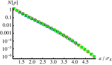
Figure 1: Scaling of the negentropy of mKE distribution for zero mean value and variable known to lie in a symmetric interval $[-a,a]$. We report the negentropy of the distribution as a function of the ratio $a/\sigma_{\scriptstyle X}$ for different values of the variance: $\sigma_{\scriptstyle X}^{2}=0.5$ (green squares), $1$ (red circles), $2$ (blue triangles).

In conclusion, we have shown that the determination of the probability distribution of a variable for which we know the first two moments and its range of variation may be effectively pursued by using the mKE. Furthermore, the negentropy of the distribution may be used to quantify how much the mKE solution differs from the MaxEnt one, i.e. to assess how the knowledge of the range of variation influences the assignment of a probability distribution. Our analysis quantitatively supports the conclusions of Ref. [4] and rigorously justifies the use of GUM-S1 recommendation also in the presence of further information on the range of variation of a quantity, namely, provided that its standard uncertainty is sufficiently small compared to the range.

References

References

- [1] BIPM, IEC, IFCC, ILAC, ISO, IUPAC, IUPAP and OIML 2008 Evaluation of Measurement Data—Supplement 1 to the Guide to the Expression of Uncertainty in Measurement—Propagation of distributions using a Monte Carlo method Joint Committee for Guides in Metrology, JCGM 101 http://www.bipm.org/utils/common/documents/jcgm/JCGM_101_2008_E.pdf
- [2] Jaynes E T 1957 Phys. Rev. 106 620; Jaynes E T 1957 Phys. Rev. 108 171
- [3] Wöger W 1987 IEEE Trans. Instr. Measurement IM-36 655658
- [4] Lira I 2009 Metrologia 46 L27
- [5] Kullback S Information theory and statistics (Wiley, New York, 1959)
- [6] Jaynes E T 1968 IEEE Trans. Systems Science and Cybernetics SSC-4 227
- [7] Olivares S and Paris M G A 2007 Phys. Rev. A 76 042120
- [8] Hyvarinen A 1998 Adv. Neural Inf. Proc. Syst. 10 273; Hyvarinen A and Oja E 2000 Neural Networks 13 411