Towards higher precision and operational use of optical homodyne tomograms

Abstract

We present the results of an operational use of experimentally measured optical tomograms to determine state characteristics (purity) avoiding any reconstruction of quasiprobabilities. We also develop a natural way how to estimate the errors (including both statistical and systematic ones) by an analysis of the experimental data themselves. Precision of the experiment can be increased by postselecting the data with minimal (systematic) errors. We demonstrate those techniques by considering coherent and photon-added coherent states measured via the time-domain improved homodyne detection. The operational use and precision of the data allowed us to check for the first time purity-dependent uncertainty relations and uncertainty relations for Shannon and Rényi entropies.

I Introduction

A measurement plays a vital role in the study of quantum physics. Optical homodyne tomography is merely one among a variety of measurement techniques, however, its importance and effectiveness can scarcely be overestimated. The conventional optical homodyne tomography of one-mode continuous-variable states takes its origin from the papers vogel-risken-1989 ; raymer ; mlynek and is instructively described in a series of books and reviews (see, e.g., leonhardt-book ; bachor-book ; lvovsky ). The original goal of the optical homodyne tomography was to infer the quantum state of light identified with the density operator $\hat{\rho}$ or the Wigner function $W(q,p)$ wigner , say. In fact, any faithfully reconstructed quasi-probability contains a complete information about the state and can then be used to calculate any characteristics of the state, for example, its purity. Unfortunately, no reconstruction procedure is perfect and, what is more unpleasant, the original errors of experimental data can grow during the reconstruction. It is generally accepted that the higher precision of the measurement, the more comprehensive information is provided and the more sophisticated phenomena can be observed. The precision is thought to be increased merely by increasing the number of experimental runs (enlarging an ensemble of identically prepared states). Clearly, such an approach leads to a reduction of statistical errors but can hardly cope with systematic ones (related with the experiment itself). On the other hand, quantum tomography is a quantitative technique only if we can evaluate the overall errors presented in the experimental data. The previous approaches do not give a direct solution of this problem: the pattern-function reconstruction can provide the statistical errors only, whereas the maximal likelihood approach to evaluation of the errors resorts to a bootstrap method whose result cannot be totally relied on and is time-consuming lvovsky . In this paper, we propose and apply in practice a straightforward method to estimate both statistical and systematic errors, thus, making a step toward a higher precision of homodyne experiments.

Our approach is based on the initial experimental data and corresponding histograms of quadrature values. The histograms are nothing else but an estimation of the quantum tomogram $w(X,\theta)$. Being a measurable characteristic of the state and describing the quantum state thoroughly, the tomogram is not only a powerful tool to reconstruct quasi-distributions but can be used solely on an equal footing (see the tomographic-probability representation of quantum mechanics mancini-manko-tombesi-1996 ; ibort-2009 ). Moreover, as we show in this paper, the tomographic approach can be used to estimate the errors of histograms and, what is more important, to calculate directly state characteristics (e.g., the purity) and their errors.

Although different kinds of photon states can be analyzed by the optical homodyne tomography, we focus our attention on photon-added states agarwal ; dodonov-manko-kor-mukh ; dodonov-2002 , whose experimental detection zavatta-science-2004 ; zavatta-pra-2005 ; zavatta-josab-2002 ; zavatta-LPL-2006 ; parigi-jpa-2009 and nonclassical behavior zavatta-pra-2007 ; kiesel-2011 were demonstrated recently. Moreover, the advanced techniques of photon addition and photon subtraction enabled us to perform a direct probe of the commutation relation between photon creation and annihilation operators parigi-science-2007 ; kim-jeong-zavatta-prl-2008 ; zavatta-prl-2009 as well as accomplish a noiseless amplification zavatta-natphot-2011 .

We use coherent (classical-like) and single-photon added coherent (non-classical) states to achieve another goal of our paper, namely, to analyze the accuracy with which the known so far fundamental quantum relations are fulfilled. Such relations include, for example, the Heisenberg inequality heisenberg and its purity-dependent version dodonov-manko-1989 as well as the state-extended uncertainty relations trifonov-2000 ; trifonov-2002 and the uncertainty relations for Shannon and Rényi entropies hirschman ; bialynicki-birula-1975 ; bialynicki-birula-2006 . It was shown theoretically in the papers manko-2009 ; denicola ; mmanko-2010 ; chernega-state-ext-1 ; chernega-2 ; mmanko-2011 how to check all these inequalities by means of the optical homodyne tomography. In this paper, we present the first experimental results for some of them. Needless to say that the accuracy of tomographic data plays the major role in this case. However, a fulfillment of the Heisenberg uncertainty relation does not mean that the quantum mechanics in its conventional form is valid (see, e.g., narcowich-oconnell ; manko-marmo-sudarshan-pla-06 ) and opens a possibility of going beyond the conventional quantum mechanics (see, e.g., thooft-2003 ; thooft-2011 ). The violation of the conventional quantum mechanics (if any) could be detected by the violation of quantum inequalities for highest moments. In principle, all the highest moments can measured via homodyne detector as well manko-physscr-2010 and the experimental check of those inequalities is to be discussed elsewhere.

The paper is organized as follows.

In Sec. II, the optical homodyne tomography is shortly reviewed with the emphasis on coherent and photon-added coherent states. Also, an optimal estimation of the quantum tomogram is developed and the influence of detection imperfection is discussed. Sec. III is devoted to the estimation of errors and a brief analysis of the reasons of systematic errors. In Sec. IV, we describe how to deal with the experimental data in an operational way by calculating the purity of the state and checking uncertainty relations mentioned above. Conclusions and prospectives are given in Sec. V.

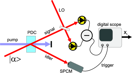
Figure 1: (Color online) Schematic of the experiment for the generation of SPACSs. An UV pulse pumps a nonlinear crystal to produce stimulated parametric down-conversion (PDC) in the mode of a seed coherent state. Detection of a single photon in the conjugated idler mode by a single-photon counting module (SPCM) heralds the successful generation of a SPACS in the signal mode, and triggers its homodyne detection. This is performed by mixing the signal state with a coherent local oscillator (LO) pulse on a 50$\%$ beam-splitter and measuring the difference photocurrent produced from two photodiodes at its outputs.

II Optical homodyne tomography

The basic idea of the homodyne tomography is to measure the quadrature operator $\hat{X}_{\theta}=\hat{Q}\cos\theta+\hat{P}\sin\theta$, where $\hat{Q}$ and $\hat{P}$ play the role of position and momentum such that $[\hat{Q},\hat{P}]=i\hbar$ and $\theta\in[0,2\pi]$ is a phase of a strong coherent light also called the local oscillator (LO). Note that $Q$ and $P$ have the same units and $\hbar$ is a constant, specified during the calibration procedure. Fixing the LO phase $\theta$, one can get access to the probability density distribution (tomogram) $w(X,\theta)=\langle X_{\theta}|\hat{\rho}|X_{\theta}\rangle$, where $\hat{X}_{\theta}|X_{\theta}\rangle=X|X_{\theta}\rangle$. If the tomographic values $w(X,\theta)$ are specified for all the points $X\in(-\infty,+\infty)$ and $\theta\in[0,\pi)$, then such an ideal tomogram contains the complete information about a quantum state.

In this section, we show how to estimate the tomogram of a coherent state and a single photon added coherent state (SPACS) in the experiment. Before we move on to the description of the experiment we briefly discuss the states under investigation.

II.1 Coherent and SPAC states

Coherent state $|\alpha\rangle$ is an eigenstate of the photon annihilation operator $\hat{a}=(\hat{Q}+i\hat{P})/\sqrt{2\hbar}$, viz., $\hat{a}|\alpha\rangle=\alpha|\alpha\rangle$, where $\alpha\in\mathbb{C}$. The coherent state $|\alpha\rangle$ is determined by the following tomogram:

$$w_{|\alpha\rangle}(X,\theta)=\tfrac{1}{\sqrt{\pi\hbar}}\exp\Big{\{}-\Big{[}\tfrac{X}{\sqrt{\hbar}}-\sqrt{2}({\rm Re}\alpha\cos\theta+{\rm Im}\alpha\sin\theta)\Big{]}^{2}\Big{\}}.$$ (1)

The SPACS is defined as $\hat{a}^{{\dagger}}|\alpha\rangle/\sqrt{1+|\alpha|^{2}}$ and its tomographic representation reads (see, e.g., korennoy )

$$w_{\hat{a}^{{\dagger}}|\alpha\rangle}(X,\theta)=\left[\sqrt{\pi\hbar}(1+|\alpha|^{2})\right]^{-1}$$

$$\times\Big{\{}2\left[\tfrac{X}{\sqrt{\hbar}}-\tfrac{1}{\sqrt{2}}({\rm Re}\alpha\cos\theta+{\rm Im}\alpha\sin\theta)\right]^{2}$$

$$\qquad+({\rm Re}\alpha\sin\theta-{\rm Im}\alpha\cos\theta)^{2}\Big{\}}$$

$$\times\exp\Big{\{}-\left[\tfrac{X}{\sqrt{\hbar}}-\sqrt{2}({\rm Re}\alpha\cos\theta+{\rm Im}\alpha\sin\theta)\right]^{2}\Big{\}}.\qquad$$ (2)

It is not hard to see that in the limit $|\alpha|\rightarrow\infty$ formula (II.1) reduces to (1), i.e. the SPACS behaves as a coherent state. A transition from a purely quantum behavior of the SPACS ($\alpha=0$) to a classical-like one ($|\alpha|\gg 1$) was also observed experimentally zavatta-science-2004 .

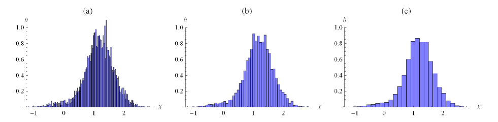
Figure 2: (Color online) Histogram $h(X,\pi)$ of a SPACS for different bin widths: (a) $b=0.025$, great statistical errors; (b) $b=0.075$; (c) $b=0.15$, larger bin widths can cause undersampling.

II.2 Experimental setup

SPACSs are generated by injecting a coherent state $|\alpha\rangle$ into the signal mode of an optical parametric amplifier and exploiting the stimulated emission of a single down-converted photon into the same mode. Successful SPACS generation takes place upon detection of a single photon in the idler mode of the amplifier. Quadrature data are then acquired by a time-domain balanced homodyne detector zavatta-josab-2002 ; zavatta-LPL-2006 triggered by such idler counts. A schematic of the setup, described in detail in zavatta-science-2004 ; zavatta-pra-2005 , is presented in Fig. 1.

Acquisition of the quadrature data from the homodyne detector is accomplished by means of a digital oscilloscope, producing a sequence of $N=5321$ quadrature values $X$ for each fixed LO phase. Calibration of $X$-values is accomplished by measuring vacuum fluctuations when the signal is blocked. In this case, $\langle X\rangle=0$ and the variance $\sigma_{XX}=\langle(X-\langle X\rangle)^{2}\rangle=\hbar/2$. Thus, a choice of $\hbar$ is rather arbitrary and we use $\hbar=\frac{1}{2}$. Once $X$ is calibrated, a state under investigation is characterized by a collection of points $\{X_{i},\theta_{j}\}$, where $i=1,\ldots,N$. The phases $\theta_{j}$ are adjusted by the piezoelectric transducer.

II.3 Tomogram estimation

The binned histogram $h(X,\theta_{j})$ is known to be constructed ambiguously because of many possibilities to choose the bin width $b$. If $b\rightarrow 0$, then the histogram is merely a sum of delta functions $\delta(X-X_{i})$. In fact, for relatively small bin widths no statistical confidence can be achieved. Conversely, if $b\rightarrow\infty$, then the histogram transforms into a flat distribution over the range of $X$, with this uniform distribution tending to zero. In this case, no useful physical information can be extracted. Needless to say that none of these two extremal types of the histogram reflects the behavior of the function $w(X,\theta)$ predicted by the theory.

Let us now derive an optimal bin width $b$ for purposes of the optical homodyne tomography. To begin with, the histogram value $h(X_{i},\theta_{j})$ at the point $X_{i}=bi$, $i\in\mathbb{Z}$, equals $N_{i}/Nb$, where $N_{i}$ is the number of measured quadrature values falling into the $i$-th bin $[X_{i},X_{i}+b)$ and $N$ is the number of all quadrature values. The statistical error of $h(X_{i},\theta_{j})$ originates from $N_{i}$ whose error is $\sqrt{N_{i}}$ because the measurement process is assumed to be Poissonian. For a fixed $N$ we naturally have $N_{i}\propto b$ (if $b$ is not too large), then the statistical error of $h(X_{i},\theta_{j})$ is $\delta h_{\rm stat}=\sqrt{h(X_{i},\theta_{j})/Nb}$. For relatively large bin widths the statistical error is negligible, however, the effect of undersampling the quadrature distribution comes into play leonhardt-1996 . The main idea is that the theoretical tomogram $w(X,\theta_{j})$ exhibits oscillating behavior with respect to $X$, with the scale of oscillations being $\sim\pi/\sqrt{2d}$, where $d$ is the number of Fock states significantly contributing to the state under investigation. The experimental histogram $h(X,\theta_{j})$ should reflect those oscillations rather than conceal them. Then, the error of undersampling for the histogram value $h(X_{i},\theta_{j})$ can be evaluated as $\delta h_{\rm und}=h(X_{i},\theta_{j})b\sqrt{2d}/\pi$. The resulting error $\delta h_{\rm stat}+\delta h_{\rm und}$ takes minimal value if $b=b_{\rm opt}\equiv[\pi/4\sqrt{2}h(X_{i},\theta_{j})Nd]^{1/3}$. Note that $b$ has the same functional dependence $\propto 1/\sqrt[3]{N}$ as the Scott’s choice $b=3.5\sigma/\sqrt[3]{N}$, where $\sigma$ is the standard deviation of $X$ scott . Note also that the optimal bin width should increase for lower values $h(X_{i},\theta_{j})$, for instance at the end of the distribution tails. For practical purposes the alternating bin widths are, however, not very convenient since they complicate data processing.

We plot some examples of histograms for different values of the bin width in Fig. 2. For our further analysis, we choose $b=0.075$ which is close to the average optimal value $b_{\rm opt}\approx 0.06$ (we put $h(X_{i},\theta_{j})\approx 1/\sqrt{2\pi}$, $N=5321$, $d\sim 1$, and scale $b_{\rm opt}$ by a factor $\sqrt{\hbar}=\frac{1}{\sqrt{2}}$). In our case, this bin width is also close to $(\max X-\min X)/\sqrt{N}\approx 0.055$ known as the square-root choice. For the normal distribution (coherent state) the Scott’s choice gives $b=0.14$ and the Sturges’ formula results in $\lceil\log_{2}N+1\rceil\approx 13$ bins ($b=0.3$). We choose $b=0.075$ to guarantee the statistical confidence and prevent the data from undersampling. The latter fact is important to observe the cases when the theoretical function $w(X,\theta)$ tends to zero in the middle of the range of $X$ as it takes place, e.g., for an ideal SPACS (see formula (II.1) with real $\alpha$ and $\theta=0$ or $\pi$).

To illustrate the estimated tomograms of a coherent state and a SPACS, we present a series of historgrams $h(X,\theta_{j})$ constructed on the basis of the experimental data with eleven LO phases $\{\theta_{j}\}_{j=1}^{11}$ within the region $[0,\pi]$ (see Fig. 3).

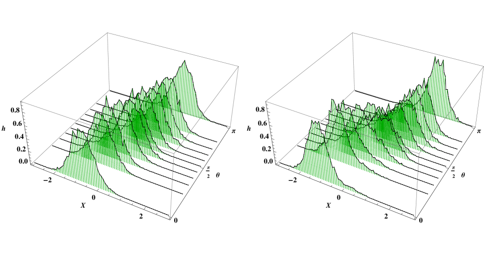
Figure 3: (Color online) Typical histograms $h(X,\theta_{j})$ of a coherent state (left) and a SPACS (right).

II.4 Detection imperfection

Let us be reminded that for a real $\alpha$ and the LO phase $\theta=0$ the tomogram (II.1) of a SPACS is $w_{\hat{a}^{{\dagger}}|\alpha\rangle}(X,0)\propto(X/\sqrt{\hbar}-\alpha/\sqrt{2})^{2}\exp[-(X/\sqrt{\hbar}-\sqrt{2}\alpha)^{2}]$ and takes on zero value if $X=\alpha\sqrt{\hbar/2}$ ($X=-\alpha\sqrt{\hbar/2}$ if $\theta=\pi$). However, one can hardly observe such property in Figs. 2 and 3. This is caused by the fact the detection efficiency $\eta<1$. The detection efficiency comprises all kinds of losses including the finite efficiency of photodetectors. Due to the imperfect detection, the measured histograms are smoothed and there is no zero point $X=\alpha\sqrt{\hbar/2}$ anymore. In fact, one actually measures not the prepared state but its convolution with a vacuum (that impinges a fictitious beamsplitter with transmittivity $\eta$ in front of an ideal quadrature detector). In terms of the Wigner fuction, the measurable state $W^{\rm det}(q,p)$ is connected with the originally prepared state $W(q^{\prime},p^{\prime})$ by the following relation:

$$W^{\rm det}(q,p) = \frac{1}{\pi(1-\eta)}\iint dq^{\prime}~{}dp^{\prime}~{}W(q^{\prime},p^{\prime})$$ (3)

$$\times\exp\left[-\frac{(q-\sqrt{\eta}q^{\prime})^{2}+(p-\sqrt{\eta}p^{\prime})^{2}}{1-\eta}\right].\quad$$

It is not hard to see that a coherent state $|\alpha\rangle$ transforms into the coherent state $|\sqrt{\eta}\alpha\rangle$ under convolution (3). On the other hand, a SPACS remains no longer a SPACS and the measurable state is given by the following Wigner function:

$$W_{\hat{a}^{{\dagger}}|\alpha\rangle}^{\rm det}(q,p)=\left[\pi(1+|\alpha|^{2})\right]^{-1}$$

$$\times\Big{\{}1+2\eta\Big{[}\Big{(}q-\tfrac{2\eta-1}{\sqrt{2\eta}}{\rm Re}\alpha\Big{)}^{2}+\Big{(}p-\tfrac{2\eta-1}{\sqrt{2\eta}}{\rm Im}\alpha\Big{)}^{2}-1\Big{]}\Big{\}}$$

$$\times\exp\left[-\left(q-\sqrt{2\eta}{\rm Re}\alpha\right)^{2}-\left(p-\sqrt{2\eta}{\rm Im}\alpha\right)^{2}\right].$$ (4)

Then, for a SPACS with real $\alpha$, the theoretical prediction of the measurable quadrature distribution is

$$\!\!\!\!\!\!w_{\hat{a}^{{\dagger}}|\alpha\rangle}^{\rm det}(X,0)=\left[\sqrt{\pi\hbar}(1+\alpha^{2})\right]^{-1}$$

$$\!\!\!\!\!\!\times\Big{[}1-\eta+2\eta\Big{(}\tfrac{X}{\sqrt{\hbar}}-\tfrac{2\eta-1}{\sqrt{2\eta}}\alpha\Big{)}^{2}\Big{]}\exp\Big{[}-\Big{(}\tfrac{X}{\sqrt{\hbar}}-\sqrt{2\eta}\alpha\Big{)}^{2}\Big{]},$$

which has no zeros and correctly describes the experimental histograms in Figs. 2 and 3.

It is worth noting that the purity of the state can reveal the detection imperfection. Although a coherent state remains pure in transformation (3), a SPACS does not. Indeed, the purity of the detectable SPACS reads

$$\mu_{\hat{a}^{{\dagger}}|\alpha\rangle}^{\rm det}=2\pi\iint dq\,dp\left[W_{\hat{a}^{{\dagger}}|\alpha\rangle}^{\rm det}(q,p)\right]^{2}=1-\frac{2\eta(1-\eta)}{(1+|\alpha|^{2})^{2}}$$ (6)

and is less than 1 whenever $0<\eta<1$ (if $\eta=0$, then the vacuum noise is only detected).

In what follows, we will concentrate on the accuracy of the experimental histograms $h^{\rm det}(X,\theta)$ and theoretical tomograms $w^{\rm det}(X,\theta)$. Thus, we will operate with the “detectable” state (not the originally prepared one). Further, we will omit the superscript ^det wherever it is clear from the context. In fact, deconvolution of formula (3) is known to be difficult to perform with experimentally given quasiprobabilities leonhardt-book and this is beyond the scope of present paper. We can refer the interested reader to the paper filippov , where a similar deconvolution problem is solved, namely, an extraction of the originally prepared microwave quantum state from a noisy output of a linear amplifier is considered.

III Accuracy of optical homodyne tomograms

Further progress of applied quantum information technologies and fundamental experiments depends greatly on the accuracy of measurement data. In optical homodyne detection of radiation field, one usually restricts oneself by the initial calibration of the detector outcomes. Namely, blocking photons of the signal mode results in the vacuum state, whose quadrature distribution is to be centered at point $X=0$ and have the dispersion $\langle X^{2}\rangle=\hbar/2$ for any phase of the local oscillator. However, in practice, a drift of the scheme parameters or an extra noise can occur during the experiment. In view of this, for practical purposes it is extremely important to trace the adequacy of the data being collected either in real time or during postprocessing. Also, the method would be beneficial if it were based on the data themselves without much additional information. In this section, we present and apply such a method.

A true tomogram $w(X,\theta)$ is known to satisfy the relation $w(X,\theta)=w(-X,\theta+\pi)$. This fact was previously used to claim that the quadrature distribution for LO phases $\theta\in[0,\pi)$ determine a quantum state thoroughly. As a result, the phases out of this range were disregarded in experiments, although they naturally provide an efficient way to check the accuracy of the data. In what follows we show that one can efficiently use the peculiar property $w(X,\theta)=w(-X,\theta+\pi)$ to check whether the data are adequate filippov-fss-11 . Moreover, one can evaluate the accuracy of the histograms.

For example, an imbalance of the optical scheme or photodetectors’ efficiencies would result in values $X$ shifted by some $x_{\rm imb}$. In this case, the distributions $w(X,\theta)$ and $w(-X,\theta+\pi)$ as functions of variable $X$ would be shifted with respect to each other by the magnitude $2x_{\rm imb}$. In case of different photodetector efficiencies, $\eta_{1}$ and $\eta_{2}$, the shift $x_{\rm imb}\propto(\eta_{1}-\eta_{2})I$, where $I$ is the LO intensity. Analogous mismatch between tomograms can take place due to a low frequency electronic noise at the input of the digital scope, the shift alternating in time.

Another reason of possible deviation of $w(X,\theta_{1})$ from $w(-X,\theta_{2})$, where $\theta_{2}$ is supposed to be equal to $\theta_{1}+\pi$, can occur due to inaccuracy in the LO phase control. Especially clearly this type of data mismatch is seen for a coherent state $|\alpha\rangle$, for which the distribution $w(X,\theta_{1})$ is shifted with respect to the distribution $w(X,\theta_{2})$ by $x_{\delta\theta}=\sqrt{2}\hbar[{\rm Re}\alpha(\cos\theta_{1}+\cos\theta_{2})+{\rm Im}\alpha(\sin\theta_{1}+\sin\theta_{2})]$ along $X$-axis. For $\theta_{1,2}=\theta\pm\delta\theta/2$, the shift $x_{\delta\theta}$ is approximately equal to $\sqrt{2}\hbar({\rm Re}\alpha\sin\theta-{\rm Im}\alpha\cos\theta)\delta\theta+\hbar({\rm Re}\alpha\cos\theta+{\rm Im}\alpha\sin\theta)\delta\theta^{2}/\sqrt{2}$.

In order to demonstrate the method above, we consider a mismatch between histograms $h(X,\pi)$ and $h(-X,0)$, which should be coincident according to the theory. Typical histograms of a SPACS are depicted in Fig. 4 for three data sets corresponding to $\sqrt{\eta}\alpha=0.64$.

One can readily notice the deviation of histograms $h(X,\pi)$ and $h(-X,0)$ for data sets #1 and #2. The shift between these histograms is evaluated as the difference between mean values of the distributions (to be precise, the shift $x=\langle X_{\pi}\rangle-\langle-X_{0}\rangle=\langle X_{\pi}\rangle+\langle X_{0}\rangle$). The experimentally determined shifts of the histogram $h(-X,0)$ with respect to $h(X,\pi)$ are summarized for coherent states and SPACS states of different intensities in Table 1.

Table 1: Shifts $x=\langle X_{\pi}\rangle+\langle X_{0}\rangle$ of the histogram $h(-X,0)$ with respect to $h(X,\pi)$ for detected coherent and SPAC states of different intensities. The amplitude $\sqrt{\eta}\alpha$ of the detected coherent state is evaluated by the experimentally measured value $(\langle X_{\pi}^{\rm coherent}\rangle-\langle X_{0}^{\rm coherent}\rangle)/2$.

Data		Detected amplitude $\sqrt{\eta}\alpha$
set		0.64	0.82	1.25	1.73
#1	coherent	0.14	0.15	$-$0.15	$-$0.17
	SPACS	0.16	0.20	$-$0.08	$-$0.10
#2	coherent	0.26	$-$0.21	0.02	0.23
	SPACS	0.26	$-$0.14	0.05	0.27
#3	coherent	0.03	$-$0.12	0.003	0.36
	SPACS	0.09	$-$0.07	0.07	0.40

While $|\alpha|$ is getting larger, one expects the error of fixing the LO phase $\delta\theta$ to get smaller (since the phase control is based on observing an interference picture which becomes clearer for larger $|\alpha|$). On the other hand, in case of real $\alpha$ and LO phase $\theta=0$, the shift $x_{\delta\theta}$ equals $\hbar\alpha\delta\theta^{2}/\sqrt{2}$ and can be non-monotonic with respect to $\alpha$ because of an additional factor.

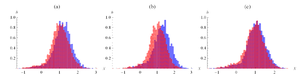
Figure 4: (Color online) Histograms $h(X,\pi)$ (blue solid lines) and $h(-X,0)$ (red dashed lines) of SPACS from first column of Table 1: (a) data set #1; (b) data set #2; (c) data set #3.

Let us now analyze how a mismatch between distributions $w(X,\theta)$ and $w(-X,\theta+\pi)$ affects the accuracy of the data and allows evaluating the experimental errors of some state characteristics.

A natural characteristic, which shows the closeness of two probability distributions $p_{1}(X)$ and $p_{2}(X)$, is the Bhattacharyya coefficient bhattacharyya defined as $B=\int\sqrt{p_{1}(X)p_{2}(X)}dX$. The Bhattacharyya coefficient $B$ equals 1 if and only if distributions $p_{1}(X)$ and $p_{2}(X)$ are identical.

Let $\rho_{1}$ be a state reconstructed from the homodyne tomograms $w(X,\theta)$, $\theta\in[0,\pi)$, and $\rho_{2}$ be a state reconstructed from the tomograms $w(X,\theta)$, $\theta\in[\pi,2\pi)$. Provided ideal tomograms the states $\rho_{1}$ and $\rho_{2}$ are identical. Experimental data result in two different states, the fidelity $F(\rho_{1},\rho_{2})={\rm Tr}\sqrt{\sqrt{\rho_{1}}\rho_{2}\sqrt{\rho_{1}}}$ between which indicates the accuracy of measured data and can be used as an estimate of the fidelity between the evaluated (reconstructed) state $\rho_{\rm est}$ and the actual state $\rho$, i.e. $F(\rho_{1},\rho_{2})\approx F(\rho,\rho_{\rm est})$. Important for us is the fact that $F(\rho_{1},\rho_{2})$ satisfies the following relation filippov-manko-distances :

$$F\leq\min_{\theta\in[0,\pi]}\int\sqrt{w(X,\theta)w(-X,\theta+\pi)}dX,$$ (7)

that is the fidelity is limited by the minimal Bhattacharyya coefficient $B_{\theta}$ for the distributions $p_{1}(X)=w(X,\theta)$ and $p_{2}(X)=w(-X,\theta+\pi)$.

In principle, formula (7) implies minimization of $B_{\theta}$ over all experimentally accessible LO phases $\theta$. In this research, we restrict ourselves by an illustration of the method of fidelity evaluation and present some values $B_{\theta=0}$ calculated for the data from the first column of Table 1: 98.70% and 98.32%, 96.20% and 95.59%, 99.67% and 99.26% for the coherent and SPAC states from data sets #1, #2, and #3, respectively. Here, we have calculated the integral (7) by replacing $w(X,\theta)\rightarrow h(X,\theta)$ and using the trapezoid method korn , with the error of calculation being $-\frac{1}{12}b^{3}\frac{d^{2}}{dX^{2}}\sqrt{w(X,0)w(-X,\pi)}<0.004\%$. Once fidelity is evaluated, one can use this knowledge to evaluate the accuracy of other state characteristics (see, e.g., dodonov-jpa-2012 ; dodonov-jrlr-2011 ).

Given tomograms $w(X,\theta)$ for two regions of the LO phases $\theta\in[0,\pi)$ and $\theta\in[\pi,2\pi)$, it is possible to evaluate the error of the mean value of any physical quantity $A$. Indeed, $\Delta A=|{\rm Tr}[(\rho_{1}-\rho_{2})A]|$, where $\rho_{1}$ and $\rho_{2}$ are defined as above. However, for some quantities one does not have to reconstruct the states and can use tomograms directly. For instance, the moment $\langle X_{\theta}^{n}\rangle=\int X^{n}w(X,\theta)dX$ is determined with the experimental error $\Delta(X_{\theta}^{n})=\int X^{n}|w(X,\theta)-w(-X,\theta+\pi)|dX$. For example, for the data set #3 from the first column of Table 1, the second moment $\langle q^{2}\rangle\equiv\langle X_{\theta=0}\rangle$ equals $\langle q^{2}\rangle=0.63\pm 0.04$ for the coherent state and $\langle q^{2}\rangle=1.23\pm 0.16$ for the SPACS. For the first moments $\langle q\rangle$ the errors are merely the shifts 0.03 and 0.09, respectively. The error bars of those quantities are of the same order for other LO phases.

To conclude this section, a relatively simple analysis of the homodyne tomographic data enables one to check their adequacy and evaluate their accuracy. As a result, one can postselect and use further only those data that meet the desired accuracy. Moreover, a mismatch between tomographic data can indicate a reason and nature of extra noise. The latter fact opens up new vistas of the optical homodyne tomography in metrology.

IV Operational use of the tomographic data

In this section, we are going to reveal some relevant information about a quantum state just using the tomographic data and circumventing a reconstruction of the density operator or the Wigner function. Also, we are checking if the data satisfy some theoretically predicted inequalities. In this section, explicit numerical values of quantities of interest are calculated for data set #3 from the first column of Table 1 which exhibits relatively small systematic errors.

IV.1 Purity

Purity $\mu={\rm Tr}\rho^{2}$ is an important state characteristic which can set some limitations on the use of the state in applications. A conventional approach to determine the state purity from the optical tomogram is to reconstruct the density matrix or the Wigner function via some improved modifications of the inverse Radon transform benichi or the maximum likelihood method hradil and then substitute them in some integral relations to calculate the purity. Recently, the state purity has been also evaluated from quadratures’ uncertainties porzio-solimeno-2011 . This method is easy to use but the evaluation gives a correct value only for Gaussian states. Here, we use the tomographic data directly and calculate the true purity without any intermediate reconstruction of the density operator or a quasiprobability distribution. Moreover, no assumption about the state being Gaussian is needed.

The purity is known to be expressed through the optical tomogram as follows omanko-2009 :

$$\mu_{\rm theor} = \frac{1}{2\pi}\int_{0}^{+\infty}dr~{}r\iint_{-\infty}^{+\infty}dXdY\,e^{-i(X+Y)r}$$ (8)

$$\times\int_{0}^{2\pi}d\theta\,w(X,\theta)w(-Y,\theta),$$

where the sequence of taking integrals is chosen for the easiest data processing. If the tomograms satisfied the relation $w(X,\theta)=w(-X,\theta+\pi)$, the calculated value of $\mu$ would be real. In fact, one would have

$$\int_{0}^{2\pi}d\theta\,w(X,\theta)w(-Y,\theta)$$

$$=\int_{0}^{\pi}d\theta\,[w(X,\theta)w(-Y,\theta)+w(-X,\theta)w(Y,\theta)]\qquad$$ (9)

and, consequently,

$$\mu = \frac{1}{\pi}\int_{0}^{+\infty}dr~{}r\iint_{-\infty}^{+\infty}dXdY\,\cos[(X+Y)r]$$ (10)

$$\times\int_{0}^{\pi}d\theta\,w(X,\theta)w(-Y,\theta).$$

The obtained formula is beneficial when the homodyne data are acquired only for the LO phases in the range $[0,\pi]$ (although it is impossible to evaluate the accuracy of $\mu$ then). As we already know, in practice the requirement $w(X,\theta)=w(-X,\theta+\pi)$ is not precisely met. Then the imaginary part of expression (8) can serve as the error bar of the purity. It can be also calculated as follows:

$$\!\!\!\!\!\!\!\Delta\mu=({\rm Tr}\rho_{1}^{2}-{\rm Tr}\rho_{2}^{2})/2$$

$$\!\!\!\!\!\!\!=\frac{1}{2\pi}\int_{0}^{+\infty}rdr\iint_{-\infty}^{+\infty}dXdY\cos[(X+Y)r]$$

$$\!\!\!\!\!\!\!\times\int_{0}^{\pi}d\theta[w(X,\theta)w(-Y,\theta)-w(X,\theta+\pi)w(-Y,\theta+\pi)].$$

Given experimental histograms $h(X,\theta_{j})$, we first calculate the sum $\frac{1}{2}\sum_{j=1}^{N_{\theta}-1}[h(X_{i},\theta_{j})h(-Y_{k},\theta_{j})+h(X_{i},\theta_{j+1})h(-Y_{k},\theta_{j+1})](\theta_{j+1}-\theta_{j})$ for any pair of bin coordinates $(X_{i},Y_{k})$, i.e. the evaluation of the function $P(X,Y)=\int_{0}^{\pi}d\theta w(X,\theta)w(-Y,\theta)$ via the trapezoid method. The error of this evaluation is roughly equal to $-\frac{1}{12}(\theta_{j+1}-\theta_{j})^{3}\frac{\partial^{2}}{\partial\theta^{2}}[w(X_{i},\theta)w(-Y_{k},\theta)]\lesssim\frac{2\pi^{2}|\alpha|^{2}}{3(N_{\theta}-1)^{3}}\exp(-X_{i}^{2}-Y_{k}^{2})\lesssim 0.003\exp(-X_{i}^{2}-Y_{k}^{2})$ for the states in question. Calculation of the integral $J(r)=\iint_{-\infty}^{+\infty}dXdY\cos[(X+Y)r]P(X,Y)$ is substituted by the calculation of the sum $\sum_{X_{i},Y_{k}}b^{2}\cos[(X_{i}+Y_{k})r]P(X_{i},Y_{k})$ for any fixed $r$. This evaluation contains two types of errors: the first one originates from the error of the function $P(X_{i},Y_{k})$ and equals $0.01e^{-r^{2}/2}$, and the second one is due to evaluation of the integral $\iint_{-\infty}^{+\infty}dXdY$ by the sum $\sum_{X_{i},Y_{k}}$ and equals $-\frac{1}{12}b^{4}\left(\frac{\partial^{2}}{\partial X^{2}}+\frac{\partial^{2}}{\partial Y^{2}}\right)\cos[(X_{i}+Y_{k})r]P(X_{i},Y_{k})\lesssim 10^{-5}(2+r^{2})$. Evaluation of the function $rJ(r)$ for the SPACS is presented in Fig. 5. Deviation of $J(r)$ from 0 for values $r>8$ is to be assigned to the second type of the error. Finally, the purity parameter (10) is calculated via integrating the function $rJ(r)$ in the range $[0,R]$, where the upper limit $R$ is chosen in such way that the integral $\mu(R):=\int_{0}^{R}rJ(r)dr$ is saturated and does not depend of $R$. The error of calculating $\mu(R)$ can be evaluated as $\Delta_{\rm calc}\mu(R)\lesssim 0.01\int_{0}^{+\infty}re^{-r^{2}/2}dr+10^{-5}\int_{0}^{R}r(2+r^{2})dr\approx 0.01+3\cdot 10^{-6}R^{4}$. We choose $R=8$ and obtain $\mu=1.00$ for the coherent state and $\mu=0.83$ for the SPACS, the error of calculation being $\Delta_{\rm calc}\mu\lesssim 0.02$. Similarly, we use formula (IV.1) to calculate the error $\Delta\mu$ originating from the inaccuracy of the original data. The direct calculation yields 0.035 for the coherent state and 0.039 for the SPACS, which is slightly greater than the error of calculation $\Delta_{\rm calc}\mu$. To resume, we obtain $\mu=1.00\pm 0.04$ and $\mu=0.83\pm 0.04$ for the coherent state and the SPACS, respectively (the overall error is estimated as $[(\Delta_{\rm calc}\mu)^{2}+(\Delta\mu)^{2}]^{1/2}$). It is worth noting that the obtained purity $\mu=0.83$ of the detected SPACS exactly coincides with what is predicted by Eq. (6) if nominal values $\eta=0.6$ and $\alpha=0.83$ are used.

We note that the errors are easily and naturally estimated in our approach in contrast to the approaches based on the density operator reconstruction that involves a rather time-consuming bootstrap method for evaluation of the errors by the maximal likelihood technique. Note that a calculation of the purity for a given density operator also results in additional calculational errors.

Figure 5: (Color online) Calculation of purity of the SPACS. The purity is the area under the curve divided by $2\pi$. Function $J(r)$ deviates from 0 for $r>8$ due to calculational errors.

IV.2 Fidelity

Usually, an experiment is aimed at producing a specific pure quantum state, $|\psi\rangle$ say. Experimentally determined quadrature distributions $w_{\rm exp}(X,\theta)$ allow calculating the fidelity $F^{2}=\langle\psi|\rho|\psi\rangle$, where $\rho$ is an actually detected state. Similarly to formula (10), we have manko-elaf-11 : $\langle\psi|\rho|\psi\rangle=\frac{1}{\pi}\int_{0}^{+\infty}r\,dr\iint_{-\infty}^{+\infty}dXdY\,\cos[(X+Y)r]\int_{0}^{\pi}d\theta\,w_{\psi}(X,\theta)w_{\rm exp}(-Y,\theta)$, where the analytical function $w_{\psi}(X,\theta)=|{\langle X_{\theta}|}{\psi\rangle}|^{2}$ is easily computed through the desired state $|\psi\rangle$. For instance, if $|\psi\rangle$ is a superposition of a finite number of Fock states $|n\rangle$, then an explicit formula for $w_{\psi}(X,\theta)$ is found, e.g., in Ref. filippov-fss-11 . Since the function $w_{\psi}(X,\theta)$ is known precisely, the error of the quantity $F^{2}$ equals $\frac{1}{2\pi}\int_{0}^{+\infty}r\,dr\iint_{-\infty}^{+\infty}dXdY\cos[(X+Y)r]\int_{0}^{\pi}d\theta\,w_{\psi}(X,\theta)[w_{\rm exp}(-Y,\theta)-w_{\rm exp}(Y,\theta+\pi)]$.

IV.3 Experimental check of uncertainty relations

IV.3.1 Heisenberg inequality

Since the main difference between two histograms $h(X,\theta)$ and $h(-X,\theta+\pi)$ is essentially the shift, the variances $\sigma_{X_{\theta}X_{\theta}}=\langle X_{\theta}^{2}\rangle-\langle X_{\theta}\rangle^{2}$ differ not so severely as the second moments. In fact, in our case we have $\Delta\sigma_{qq}=0.004$ for the coherent state and $0.013$ for the SPACS.

In this subsection, we are going to check if the Heisenberg uncertainty relation $\sigma_{qq}\sigma_{pp}\geq\hbar^{2}/4$ holds true and what is the extent to which it is fulfilled. Certainly, thanks to the initial calibration of the apparatus by the vacuum state, we can adjust $\hbar=\frac{1}{2}$ and check the inequality for any other states but not the vacuum itself. The errors of determining second moments are evaluated as described in Sec. III.

For the coherent state we have $\sigma_{qq}\sigma_{pp}=0.0612\pm 0.0014$, which coincides with $0.0625$ within the error bar. For the SPACS we obtain $\sigma_{qq}\sigma_{pp}=0.101\pm 0.006>0.0625$. The coherent state has the minimal uncertainty indeed and, therefore, is pure. This result is in agreement with the detection imperfection discussed in Sec. II.4 because the imperfect detection results in $|\alpha\rangle\rightarrow|\sqrt{\eta}\alpha\rangle$, i.e. the pure coherent state is transformed into another pure coherent state which exhibits the same minimal uncertainty. In fact, this observation confirms the validity of using vacuum state for the initial calibration.

There exists, however, a stronger version of the Heisenberg uncertainty relation which takes into account the purity of the state, namely,

$$\sigma_{qq}\sigma_{pp}\geq\hbar^{2}\Phi^{2}(\mu)/4,$$ (12)

which is also known as purity-dependent uncertainty relation dodonov-manko-1989 . Here, the purity-dependent function $\Phi(\mu)=2-\sqrt{2\mu-1}$ if $\frac{5}{9}\leq\mu\leq 1$ and $\Phi(\mu)\approx(4+\sqrt{16+9\mu^{2}})/9\mu\pm 4\%$ within the whole range $\mu\in(0,1]$. Employing the previously found values of the purity (Sec. IV.1), the inequality (12) transforms into $0.101\pm 0.006\geq 0.085\pm 0.006$ for the SPACS, which is the first direct experimental verification of formula (12) within the accuracy $\sim 3\sigma$. This result also encourages a feasible verification of two-mode uncertainty relations manko-ventriglia-2012 because the corresponding methods of detecting two-mode states by a single homodyne detector are already available solimeno .

IV.3.2 State-extended uncertainty relation

Recently, Trifonov generalized uncertainty relations for a pair of different states trifonov-2000 ; trifonov-2002 , where the variances of one state were connected with the variances of the other by a series of so-called state-extended uncertainty relation. One of such relations reads

$$\tfrac{1}{2}\big{(}\sigma_{qq}^{(1)}\sigma_{pp}^{(2)}+\sigma_{qq}^{(2)}\sigma_{pp}^{(1)}\big{)}\geq\tfrac{\hbar^{2}}{4}.$$ (13)

We associate states “1” and “2” with the coherent state and the SPACS, respectively. Using the experimental data, the relation (13) takes the form $0.160\pm 0.006>0.0625$, and thus is fulfilled with a great margin. The great margin is due to the fact that “1” is a coherent state for which $\sigma_{qq}=\sigma_{pp}=\hbar/2$. This first demonstration of state-extended uncertainty relation can encourage its further applications to other states saturating it (e.g., some squeezed states).

IV.4 Experimental check of entropic relations

IV.4.1 Shannon entropy

Given a wavefunction $\psi(q)$ of some pure state and the wavefunction $\tilde{\psi}(p)$ of the same state in the momentum representation, we are aware that they are not independent and are related by the Fourier transform. In view of this, the narrower the distribution $|\psi(q)|^{2}$ the wider $|\tilde{\psi}(p)|^{2}$ is and vice versa. It means that the entropies $S_{q}=-\int|\psi(q)|^{2}\ln|\psi(q)|^{2}dq$ and $S_{p}=-\int|\tilde{\psi}(p)|^{2}\ln|\tilde{\psi}(p)|^{2}dp$ cannot take small values simultaneously and turn out to satisfy the following relation bialynicki-birula-1975 :

$$S_{q}+S_{p}\geq\ln(\pi\hbar)+1,$$ (14)

which is also valid in case of mixed states, with $|\psi(q)|^{2}$ and $|\tilde{\psi}(p)|^{2}$being replaced by the marginal distributions $w(X,0)$ and $w(X,\frac{\pi}{2})$, respectively. Since quadrature operators $\hat{X}_{\theta}$ and $\hat{X}_{\theta+\pi/2}$ satisfy the same commutation relation as $\hat{q}$ and $\hat{p}$ do, one can readily generalize (14) and write denicola ; mmanko-2010 ; mmanko-2011

$$S(\theta)+S(\theta+\pi/2)\geq\ln(\pi\hbar)+1,$$ (15)

where $S(\theta)\equiv S_{X_{\theta}}$ and the right-hand side equals 1.45 if $\hbar=\tfrac{1}{2}$. The inequality (15) holds true for all LO phases $\theta$. Considering $\theta$ as an additional independent variable, one can now integrate (15) over $\theta\in[0,\pi]$. Taking into account that the theoretical tomogram satisfies $w(X,\theta)=w(-X,\theta+\pi)$, we obtain

$$2\int_{0}^{\pi}S(\theta)\frac{d\theta}{\pi}\geq\ln(\pi\hbar)+1$$ (16)

or, equivalently,

$$H_{X,\theta} \equiv -\int_{-\infty}^{+\infty}dX\int_{0}^{\pi}\frac{d\theta}{\pi}~{}w(X,\theta)\ln w(X,\theta)$$ (17)

$$\geq \tfrac{1}{2}\left[\,\ln(\pi\hbar)+1\right],$$

where $H_{X,\theta}$ can be treated as the conventional Shannon entropy of the probability distribution function $w(X,\theta)$ of two random variables $X\in(-\infty,+\infty)$ and $\theta\in[0,\pi]$ such that $\frac{1}{\pi}\int_{-\infty}^{+\infty}dX\int_{0}^{\pi}d\theta~{}w(X,\theta)=1$. A similar treatment of the quantum homodyne tomography as an informationally complete positive operator-valued measure on $[0,2\pi]\times\mathbb{R}$ is presented in the paper albini-devito-toigo . From the viewpoint of foundations of quantum mechanics, a quantum state is defined by a fair probability distribution function $w(X,\theta)$ of two random variables (a point in the simplex of infinite dimension) such that its entropy necessarily satisfies the relation (17).

The evaluation of the integral (16) is performed by a trapezoid method, i.e. $2\int_{0}^{\pi}S(\theta)\frac{d\theta}{\pi}\approx\sum_{j=1}^{N_{\theta}-1}(\theta_{j+1}-\theta_{j})[S(\theta_{j})+S(\theta_{j+1})]$. The evaluation of $S(\theta_{j})$, in its turn, is performed by substituting the experimental binned histogram $h(X,\theta_{j})$ for $w(X,\theta)$.

The finite bin width $b$ is known to affect the right-hand side of the relation (15) (see rudnicki and references therein). If we take the bin width $b=0.075$ and the cutoff value of $X$ equal to 3, then the right-hand side of (15) is to be diminished by $0.03$ and equals $1.42$ for the choice $\hbar=\frac{1}{2}$. In fact, the allowance is always negative and vanishes for larger cutoffs because the states of our interest are localized quite close to center of the phase space. Using quadratures $X_{\theta=0}$ and $X_{\theta=\pi/2}$, we calculate the left-hand side of (14) and the result is $1.43\pm 0.01$ for the coherent state and $1.65\pm 0.03$ for the SPACS, where the errors are evaluated by comparing the experimental values $S(\theta)$ and $S(\theta+\pi)$. The coherent state saturates the boundary as it is predicted by the theory bialynicki-birula-1975 .

As to integral relation (16), the experimental data yield the following quantities of the left hand side of (16): $1.42\pm 0.01$ for the coherent state and $1.70\pm 0.03$ for the SPACS, where the error bars comprise both the error of calculation and the errors of the experimental data.

IV.4.2 Rényi entropy

The Rényi entropy of the probability distribution $p(X)$ is defined through $R_{\beta}[p(X)]=(1-\beta)^{-1}\ln\int p^{\,\beta}(X)dX$ and represents nothing else but a one-parametric family of entropy measures renyi . The Rényi entropy reduces to the Shannon entropy in the limit $\beta\rightarrow 1$. For $\beta>1$ there exists a conjugate parameter $\gamma$ such that $\beta^{-1}+\gamma^{-1}=2$. We can put $\beta=(1-r)^{-1}$ and $\gamma=(1+r)^{-1}$, where $r\in(0,1)$. An analog of the relation (14) in terms of the Rényi entropy is $R_{\beta}[w(X,0)]+R_{\gamma}[w(X,\frac{\pi}{2})]\geq\ln(\pi\hbar)-\frac{1}{2}[(1-\beta)^{-1}\ln\beta+(1-\gamma)^{-1}\ln\gamma]$. In terms of a single parameter $r$ this relation takes the form mmanko-2011

$$\!\!\!\!\!\mathcal{R}(r)\equiv\frac{1+r}{r}\ln\left\{\int[w(X,0)]^{(1+r)^{-1}}dX\right\}$$

$$\!\!\!\!\!-\frac{1-r}{r}\ln\left\{\int[w(X,\tfrac{\pi}{2})]^{(1-r)^{-1}}dX\right\}$$

$$\!\!\!\!\!\geq\ln(\pi\hbar)+\tfrac{1}{2r}[(1+r)\ln(1+r)-(1-r)\ln(1-r)],\qquad$$ (18)

which remains true by replacing $w(X,0)$ and $w(X,\frac{\pi}{2})$ by $w(X,\theta)$ and $w(X,\frac{\pi}{2}+\theta)$, respectively. For the sake of simplicity, we concentrate on the experimental check of inequality (IV.4.2) for $r\in(-1,1)$. The results are presented in Fig. 6, where the points correspond to the left-hand side of (IV.4.2) calculated via the experimental histograms. As above, the coherent state saturates the boundary (within the experimental errors) and the experimentally determined values are symmetrical with respect to change $r\rightarrow-r$ because the position and momentum are identically distributed. This does not take place for the SPACS and such an asymmetry is readily seen.

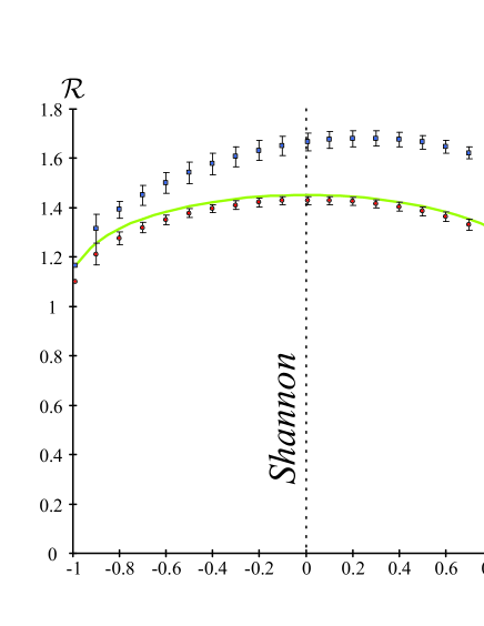
Figure 6: (Color online) Experimental check of uncertainty relations for the Rényi entropy (IV.4.2). Filled circles and squares correspond to experimental coherent and SPAC states, respectively (for points without error bars the corresponding errors are greater than 1). Solid line is a theoretical bound. When $r\rightarrow 0$ the inequality (IV.4.2) transforms into the inequality for the Shannon entropy (14).

V Summary

In this paper, we have considered a relatively simple but extremely powerful experimental apparatus to measure quantum states of light – homodyne detector. Our main idea was to use measurable quantities (histograms) to reveal as much information about light states as possible. First, the measured histograms enabled us to estimate the optical tomogram, i.e. the quantum state itself. We developed a method for choosing an optimal bin width, which ensures statistical confidence and prevents from undersampling at the same time. Second, we managed to accomplish a quantitative analysis of the accuracy of estimated tomograms by using the peculiar property of fair tomograms $w(X,\theta)=w(-X,\theta+\pi)$. Distinction of our approach is that the evaluated errors comprise both statistical and systematical errors. Moreover, the detailed analysis can also reveal probable sources of systematical errors such as imprecision of the LO phase control, which is hardly possible to detect by other methods. Even if the systematic error cannot be got rid of, one can use an original collection of experimental data to postselect those data which exhibit the least systematic error. Third, we used the measurable quantities (histograms) to calculate the characteristics of the state directly. For instance, the purity and its error are naturally calculated on the basis of measured experimental data without any time-consuming state-reconstruction procedure with controversial error estimation. Our data result in the relative error about several percent (1$\div$5%) for almost all state characteristics (when their theoretical values do not vanish). Last but not least, the operational use of the data allowed us to check for the first time the fundamental properties of quantum objects such as the (purity-dependent) uncertainty relations for position and momentum as well as their entropic analogs.

To conclude, we believe that the developed methods will contribute to achieving a higher precision of optical homodyne detection and encourage the operational use of experimental data, which can turn out to be crucial for the analysis of multimode quantum states.

- (1) K. Vogel and H. Risken, Phys. Rev. A 40, 2847 (1989).
- (2) D. T. Smithey, M. Beck, M. G. Raymer, and A. Faridani, Phys. Rev. Lett. 70, 1244 (1993).
- (3) S. Schiller, G. Breitenbach, S. F. Pereira, T. Müller, and J. Mlynek, Phys. Rev. Lett. 77, 2933 (1996).
- (4) U. Leonhardt, Measuring the Quantum State of Light (Cambridge University Press, Cambridge, 1997).
- (5) H.-A. Bachor and T. C. Ralph, A Guide to Experiments in Quantum Optics, 2nd ed. (WILEY-VCH Verlag, Weinheim, 2004).
- (6) A. I. Lvovsky and M. G. Raymer, Rev. Mod. Phys. 81, 299 (2009).
- (7) E. Wigner, Phys. Rev. 40, 749 (1932).
- (8) S. Mancini, V. I. Man’ko, and P. Tombesi, Phys. Lett. A 213, 1 (1996).
- (9) A. Ibort, V. I. Man’ko, G. Marmo, A. Simoni, and F. Ventriglia, Phys. Scr. 79, 065013 (2009).
- (10) G. S. Agarwal and K. Tara, Phys. Rev. A 43, 492 (1991).
- (11) V. V. Dodonov, M. A. Marchiolli, Ya. A. Korennoy, V. I. Man’ko, and Y. A. Moukhin, Phys. Rev. A 58, 4087 (1998).
- (12) V. V. Dodonov, J. Opt. B: Quantum Semiclass. Opt. 4, R1 (2002).
- (13) A. Zavatta, S. Viciani, and M. Bellini, Science 306, 660 (2004).
- (14) A. Zavatta, S. Viciani, and M. Bellini, Phys. Rev. A 72, 023820 (2005).
- (15) A. Zavatta, M. Bellini, P. L. Ramazza, F. Marin, and F. T. Arecchi, J. Opt. Soc. Am. B 19 1189 (2002).
- (16) A. Zavatta, S. Viciani, and M. Bellini, Laser Phys. Lett. 3, 3 (2006).
- (17) V. Parigi, A. Zavatta, and M. Bellini, J. Phys. B: At. Mol. Opt. Phys. 42, 114005 (2009).
- (18) A. Zavatta, V. Parigi, and M. Bellini, Phys. Rev. A 75, 052106 (2007).
- (19) T. Kiesel, W. Vogel, M. Bellini, and A. Zavatta, Phys. Rev. A 83, 032116 (2011).
- (20) V. Parigi, A. Zavatta, M. Kim, and M. Bellini, Science 317, 1890 (2007).
- (21) M. S. Kim, H. Jeong, A. Zavatta, V. Parigi, and M. Bellini, Phys. Rev. Lett. 101, 260401 (2008).
- (22) A. Zavatta, V. Parigi, M. S. Kim, H. Jeong, and M. Bellini, Phys. Rev. Lett. 103, 140406 (2009).
- (23) A. Zavatta, J. Fiurášek, and M. Bellini, Nature Photonics 5, 52 (2011).
- (24) W. Heisenberg, Ztschr. Phys. 43, 172 (1927).
- (25) V. V. Dodonov and V. I. Man’ko. Generalization of uncertainty relation in quantum mechanics, vol. 183 of Invariants and the Evolution of Nonstationary Quantum Systems, Proc. P N Lebedev Physical Institute, Nova Science, New York (1989).
- (26) D. A. Trifonov, J. Phys. A: Math. Gen. 33, L299 (2000).
- (27) D. A. Trifonov, Eur. Phys. J. B 29, 349 (2002).
- (28) I. I. Hirschman, American Journal of Mathematics 79, 152 (1957).
- (29) I. Blalynicki-Birula and J. Mycielski, Commun. Math. Phys. 44, 129 (1975).
- (30) I. Bialynicki-Birula, Phys. Rev. A 74, 052101 (2006).
- (31) V. I. Man’ko, G. Marmo, A. Simoni, and F. Ventriglia, Advanced Science Letters 2, 517 (2009).
- (32) V. N. Chernega and V. I. Man’ko, J. Russ. Laser Res. 32, 125 (2011).
- (33) V. N. Chernega, Phys. Scr. T147 014006 (2012).
- (34) S. De Nicola, R. Fedele, M. A. Man’ko, and V. I. Man’ko, Eur. Phys. J. B 52, 191 (2006).
- (35) M. A. Man’ko, Phys. Scr. 82, 038109 (2010).
- (36) M. A. Man’ko and V. I. Man’ko, Found. Phys. 41, 330 (2011).
- (37) F. J. Narcowich and R. F. O’Connell, Phys. Rev. A 34, 1 (1986).
- (38) O. V. Man’ko, V. I. Man’ko, G. Marmo, E. C. G. Sudarshan, and F. Zaccaria, Phys. Lett. A 357, 255 (2006).
- (39) G. ’t Hooft, Int. J. Theor. Phys. 42, 355 (2003).
- (40) G. ’t Hooft, How a wave function can collapse without violating Schrödinger s equation, and how to understand Born s rule, arXiv:1112.1811v2 [quant-ph] (2011).
- (41) V. I. Man’ko, G. Marmo, A. Simoni, and F. Ventriglia, Phys. Scr. 82, 038114 (2010).
- (42) Ya. A. Korennoy and V. I. Man’ko, Phys. Rev. A 83, 053817 (2011).
- (43) U. Leonhardt, M. Munroe, T. Kiss, Th. Richter, and M. G. Raymer, Opt. Commun. 127, 144 (1996).
- (44) D. W. Scott, Biometrika 66, 605 (1979).
- (45) S. N. Filippov and V. I. Man’ko, Phys. Rev. A 84, 033827 (2011).
- (46) S. N. Filippov and V. I. Man’ko, Phys. Scr. 83, 058101 (2011).
- (47) A. Bhattacharyya, Bull. Calcutta Math. Soc. 35, 99 (1943).
- (48) S. N. Filippov and V. I. Man’ko, Phys. Scr. T140, 014043 (2010).
- (49) G. A. Korn and T. M. Korn. Mathematical Handbook for Scientists and Engineers. Definitions, Theorems, and Formulas for Reference and Review, 2nd enlarged and revised edition (McGraw-Hill, New York, 1968).
- (50) V. V. Dodonov, J. Phys. A: Math. Theor. 45, 032002 (2012).
- (51) V. V. Dodonov, J. Russ. Laser Res. 32, 412 (2011).
- (52) H. Benichi and A. Furusawa, Phys. Rev. A 84, 032104 (2011).
- (53) Z. Hradil, Phys. Rev. A 55, R1561 (1997).
- (54) V. I. Man’ko, G. Marmo, A. Porzio, S. Solimeno, and F. Ventriglia, Phys. Scr. 83, 045001 (2011).
- (55) O. V. Man’ko and V. I. Man’ko, Fortschr. Phys. 57, 1064 (2009).
- (56) M. A. Man’ko and V. I. Man’ko, AIP Conference Proceedings 1334, 217 (2011)
- (57) V. I. Man’ko, G. Marmo, A. Simoni, and F. Ventriglia, Phys. Scr. T147, 014021 (2012).
- (58) V. D’Auria, S. Fornaro, A. Porzio, S. Solimeno, S. Olivares, and M. G. A. Paris, Phys. Rev. Lett. 102, 020502 (2009).
- (59) P. Albini, E. De Vito, and A. Toigo, J. Phys. A: Math. Theor. 42, 295302 (2009).
- (60) Ł. Rudnicki, J. Russ. Laser Res. 32, 393 (2011).
- (61) A. Rényi. Probability Theory (North-Holland, Amsterdam, 1970).