Dynamic Compression-Transmission for Energy-Harvesting Multihop Networks with Correlated Sources

Abstract

Energy-harvesting wireless sensor networking is an emerging technology with applications to various fields such as environmental and structural health monitoring. A distinguishing feature of wireless sensors is the need to perform both source coding tasks, such as measurement and compression, and transmission tasks. It is known that the overall energy consumption for source coding is generally comparable to that of transmission, and that a joint design of the two classes of tasks can lead to relevant performance gains. Moreover, the efficiency of source coding in a sensor network can be potentially improved via distributed techniques by leveraging the fact that signals measured by different nodes are correlated.

In this paper, a data gathering protocol for multihop wireless sensor networks with energy harvesting capabilities is studied whereby the sources measured by the sensors are correlated. Both the energy consumptions of source coding and transmission are modeled, and distributed source coding is assumed. The problem of dynamically and jointly optimizing the source coding and transmission strategies is formulated for time-varying channels and sources. The problem consists in the minimization of a cost function of the distortions in the source reconstructions at the sink under queue stability constraints. By adopting perturbation-based Lyapunov techniques, a close-to-optimal online scheme is proposed that has an explicit and controllable trade-off between optimality gap and queue sizes. The role of side information available at the sink is also discussed under the assumption that acquiring the side information entails an energy cost. It is shown that the presence of side information can improve the network performance both in terms of overall network cost function and queue sizes.

I Introduction

Wireless sensor networks have found applications in a large number of fields such as environmental sensing and structural health monitoring [Dargie10]. In such applications, the maintenance necessary to replace the batteries when depleted is often of prohibitive complexity, if not impossible. Therefore, sensors that harvest energy from the environment, e.g., in the form of solar, thermal, vibrational or radio energy [Paradiso05] [Conrad08], have been proposed and are now commercially available.

Given the interest outlined above, the problem of designing optimal transmission protocols for energy harvesting wireless sensor networks has recently received considerable attention. In the available body of work reviewed below in Section I-B, the only source of energy expenditure is the energy used for transmission. This includes, e.g., the energy used by the power amplifiers. However, a distinguishing feature of sensor networks is that the sensors have not only to carry out transmission tasks, but also sensing and source coding tasks, such as compression. The source coding tasks entail a non-negligible energy consumption. In fact, reference [Barr06] demonstrates that the overall cost required for compression is comparable with that needed for transmission, and that a joint design of the two tasks can lead to significant energy saving gains. Another distinguishing feature of sensor networks is that the efficiency of source coding can be improved via distributed source coding techniques (see, e.g., [ElGamal12]) by leveraging the fact that sources measured by different sensors are generally correlated (see, e.g., [Zordan11]).

I-A Contributions

In this paper, we focus on an energy-harvesting wireless sensor network and account for the energy costs of both source coding and transmission. Moreover, we assume that the sensors can perform distributed source coding to leverage the correlation of the sources measured at different sensors. A key motivation for enabling distributed source coding in energy-harvesting networks is that this enables sensors with correlated measurements to trade energy resources among them, to an extent determined by the amount of correlation. For instance, a sensor that is running low on energy can benefit from the energy potentially available at a nearby node if the latter has correlated measurements. This is because, through distributed source coding, the transmission requirements on the first sensor are eased by the transmission of correlated information from the nearby sensor.

We study the problem of dynamically and jointly optimizing the source coding and transmission strategies over time-varying channels and sources. The problem consists in the minimization of a cost function of the distortions in the source reconstructions at the sink under queue stability constraints. Our approach is based on the Lyapunov optimization strategy with weight perturbation developed in [Huang10]. We devise an efficient online algorithm that only takes actions based on the harvested energy, on the current state of channel, queues and energy reserves, and also based on the statistical description of the source correlation. We prove that the proposed policy achieves an average network cost that can be made arbitrarily close to the optimal one with a controllable trade-off between the sizes of the queues and batteries.

We also investigate the role of side information available at the sink under the assumption that acquiring the side information entails an energy cost. It is shown that properly allocating the available (harvested) energy to both the tasks of transmission and side information measurement has significant benefits both in terms of overall network cost function and queue sizes.

I-B Prior Work

We start by introducing related prior work that assumes energy harvesting. The literature on this topic is quickly increasing in volume but it mostly (with the exception of [Castiglione11]) accounts only for the energy consumption of the transmission component, and does not model the contribution of the source coding part. In this context, references [Ozel11] and [Keong11] studied the problem of maximizing the throughput or minimizing the completion time for a single link energy-harvesting system by focusing on both offline and online policies (see also [Devillers11, Chen11]). A related work is also reference [Sharma10] that finds a power allocation policy that stabilizes the data queue whenever feasible. Still, for a point-to-point system, using large deviation tools, the effect of finite data queue length and battery size is studied in [Srivastava10] in terms of scaling results as the battery and queue grow large. We now consider work on multihop energy-harvesting networks. As mentioned above, all the works at hand only account for the energy used for transmission. Moreover, source correlations and distributed source coding are not accounted for. In [Huang10] assuming independent and identically distributed (i.i.d.) channel states and energy harvesting processes, a Lyapunov optimization technique with weight perturbation [Huang11] is leveraged to obtain approximately optimal strategies in terms of a general function of the data rates under queue stability constraints. The proposed technique obtains an explicit trade-off in terms of data queue length and battery size. An extension of this work that assumes more general arrival, channel state and recharge processes along with finite batteries and queues is put forth in [Mao11]. Also related are [Gratzianas10], [Lin07] and [Lin07_2] that tackle similar problems.

We now discuss work that accounts for the energy trade-offs related to source coding and transmission. These works (except [Castiglione11]) do not model the additional constraints arising from energy harvesting. Moreover, they do not allow for distributed source coding. The joint design of source coding and transmission parameters is investigated through various algorithms, for either static scenarios in [Luna03, Akyol08] or dynamic scenarios in [Neely08, Sharma09]. Specifically, references [Neely08] and [Sharma09] studied the trade-offs between energy used for compression, or more generally source coding, and transmission by assuming i.i.d. source and channel processes and arbitrarily large data buffer. Using Lyapunov optimization techniques, a policy with close-to-optimal power expenditure and an explicit trade-off with the delay is derived for a given average distortion. The problem of optimal energy allocation between source coding and transmission for a point-to-point system was studied in [Castiglione11].

Finally, distributed source coding techniques for multihop sensor networks has been studied in [Cristescu06] and [Cui07]. In [Cristescu06], the problem of optimizing the transmission and compression strategy was tackled under distortion constraints in a centralized fashion, whereas [Cui07] proposes a distributed algorithm that maximizes an aggregate utility measure defined in terms of the distortion levels of the sources. Both these works do not consider energy harvesting nor the energy consumption of the sensing process.

I-C Paper organization

The rest of the paper is organized as follows. In Section II we present the system model and we state the optimization problem. In Section III we obtain a lower bound on the optimal network cost for the proposed problem. In Section IV we present the proposed algorithm designed following the Lyapunov optimization framework and we show how it can be implemented in a distributed fashion. Section LABEL:sec:performance formalizes the main results of our paper and provide analytical insights into the performance of the proposed policy. Section LABEL:sec:side_information proposes an extended version of the problem, where the sink node acts as a cluster head that is able to acquire correlated side information to improve the system performance. In Section LABEL:sec:results we prove the effectiveness of our analytical analysis and discuss the impact of the optimization parameters. Section LABEL:sec:conclusions concludes the paper.

II System model

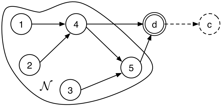
Figure 1: A set ${\mathcal{N}}$ of energy-harvesting nodes communicate correlated sources to a destination $d$. For the more general model of Section LABEL:sec:side_information, the destination $d$ acts as a cluster head and communicates to a network collector node (shown in dashed lines). In this latter model, the node $d$ can collect side information correlated to the sources measured by the nodes.

We consider a wireless network modeled by a direct graph ${\mathcal{G}}=({\mathcal{N}}\cup\{d\},{\mathcal{L}})$, where ${\mathcal{N}}=\left\{1,2,\ldots,N\right\}$ is the set of nodes in the network, $d$ is the destination (or sink), and ${\mathcal{L}}\subset\{(n,m)\text{: }n,m\in{\mathcal{N}}\cup\{d\},n\neq m\}$ represents the set of communication links, see Fig. 1 for an illustration. We define ${l_{\rm max}}$ as the maximum number of transmission links that any node $n\in{\mathcal{N}}\cup\{d\}$ can have. As discussed below, we allow for fairly general interference models. We will consider a more general model in Section LABEL:sec:side_information in which the sink acts as a cluster head for the set of nodes ${\mathcal{N}}$, and reports to a collector node $c$ (see Fig. 1).

II-A Transmission Model

The transmission model follows the framework of, e.g., [Georgiadis06]. According to this model, the network operates in slotted time and, at every time slot $t=1,2,\ldots$, each node $n\in{\mathcal{N}}$ allocates power $P_{n,m}(t)\geq 0$ to each outgoing link $(n,m)\in{\mathcal{L}}$ for data transmission. In what follows, we refer to the number of channel uses (or transmission symbols) per time slot as the baud rate multiplied by the slot duration. At the generic time slot $t$ we define ${\mathbf{P}}(t)=\{P_{n,m}(t)\}$, with $(n,m)\in{\mathcal{L}}$, as the power allocation matrix and the total transmission power of node $n$, that is

$$P_{n}(t)=\sum_{m\text{: }(n,m)\in{\mathcal{L}}}P_{n,m}(t),$$ (1)

which is assumed to satisfy the constraint $P_{n}(t)\leq{P_{\rm max}}$, for some ${P_{\rm max}}<\infty$. The transmission rate $\mu_{n,m}(t)$ on link $(n,m)$ depends on the power allocation matrix ${\mathbf{P}}(t)$ and on the current channel state ${\textbf{S}}(t)=\{S_{n,m}(t)\}$ with $(n,m)\in{\mathcal{L}}$. The latter accounts, for instance, for the current fading channels or for the connectivity conditions on the network links. We assume that ${\textbf{S}}(t)$ takes values in some finite set ${\mathcal{S}}=({\textbf{s}}_{1},{\textbf{s}}_{2},\ldots,{\textbf{s}}_{M})$, is constant within a time slot, but is independent and identically distributed (i.i.d.) across time slots. We use $\rho_{{\textbf{s}}_{i}}=\Pr\left[{\textbf{S}}(t)={\textbf{s}}_{i}\right]$ for $i=1,\ldots,M$. We write

$$\mu_{n,m}(t)={\mathrm{C}}_{n,m}({\mathbf{P}}(t),{\textbf{S}}(t)),$$ (2)

where ${\mathrm{C}}_{n,m}({\mathbf{P}}(t),{\textbf{S}}(t))$ is the capacity-power curve for link $(n,m)$ expressed in terms of bits per channel use (transmission symbol). The latter depends on the specific network transmission strategy, which includes the modulation and coding/decoding schemes used on all links. We assume that function ${\mathrm{C}}_{n,m}({\mathbf{P}}(t),{\textbf{S}}(t))$ is continuous in ${\mathbf{P}}(t)$ and non decreasing in $P_{n,m}(t)$. An example of the function ${\mathrm{C}}_{n,m}({\mathbf{P}}(t),{\textbf{S}}(t))$ is the Shannon capacity obtained by treating interference as noise at the receivers, namely

$$\begin{split}{\mathrm{C}}_{n,m}({\mathbf{P}}&(t),{\textbf{S}}(t))\propto\log\left(1+\frac{P_{n,m}(t)S_{n,m}(t)}{N_{0}+\sum_{(l,n)\in{\mathcal{L}}}P_{l}(t)S_{l,n}(t)}\right),\end{split}$$ (3)

where $S_{n,m}(t)$ represents the channel power gain on link $(n,m)$ and $N_{0}$ is the noise spectral density. We assume that there exists some finite constant ${\mu_{\rm max}}$ such that $\mu_{n,m}(t)\leq{\mu_{\rm max}}$ for all $t$, any power allocation vector ${\mathbf{P}}(t)$ and channel state ${\textbf{S}}(t)$. Moreover, following [Huang10], we assume that the function ${\mathrm{C}}_{n,m}({\mathbf{P}}(t),{\textbf{S}}(t))$ satisfies the following properties:

Property 1: For any power allocation matrix ${\mathbf{P}}(t)$, we have:

$${\mathrm{C}}_{n,m}({\mathbf{P}}(t),{\textbf{S}}(t))\leq\xi P_{n,m}(t),$$ (4)

for some finite constant $\xi>0$;

Property 2: For any power allocation matrix ${\mathbf{P}}(t)$ and matrix ${\mathbf{P}}^{\prime}(t)$ obtained by ${\mathbf{P}}(t)$ by setting the entry $P_{n,m}(t)$ to zero for a given $(n,m)$ pair, we have:

$${\mathrm{C}}_{a,b}({\mathbf{P}}(t),{\textbf{S}}(t))\leq{\mathrm{C}}_{a,b}({\mathbf{P}}^{\prime}(t),{\textbf{S}}(t)),$$ (5)

for all $(a,b)\in{\mathcal{L}}$, with $(a,b)\neq(n,m)$.

Note that both properties are satisfied by typical choices of function ${\mathrm{C}}_{n,m}({\mathbf{P}}(t),{\textbf{S}}(t))$ such as (3). In fact, Property 1 is satisfied if function ${\mathrm{C}}_{n,m}({\mathbf{P}}(t),{\textbf{S}}(t))$ is concave with respect to $P_{n,m}(t)$, while Property 2 states that interference due to power spent on other links cannot be beneficial. Finally, we define the total outgoing transmission rate ${\mu_{n,*}}(t)$ from a node $n\in{\mathcal{N}}$ at time $t$ as

$${\mu_{n,*}}(t)=\sum_{m\text{: }(n,m)\in{\mathcal{L}}}\mu_{n,m}(t),$$ (6)

and the total incoming transmission rate ${\mu_{*,n}}(t)$ at a node $n\in{\mathcal{N}}$ as

$${\mu_{*,n}}(t)=\sum_{m\text{: }(m,n)\in{\mathcal{L}}}\mu_{m,n}(t).$$ (7)

II-B Data Acquisition, Compression and Distortion Model

At each time slot, each node of the network is able to sense the environment and to acquire spatially correlated measurements. The measurements are then routed through the network to be gathered by a sink node, as illustrated in Fig. 1. Before transmission, the acquired data is compressed via adaptive lossy source coding by leveraging the spatial correlation of the measurements. Specifically, we define the source state at time $t$ as the spatial correlation matrix describing the signal within this time slot, which is referred to as ${\textbf{O}}(t)=\{O_{n,m}(t)\}$ with $n,m\in{\mathcal{N}}$. We assume that ${\textbf{O}}(t)$ takes values in some finite set ${\mathcal{O}}=\{{\textbf{o}}_{1},{\textbf{o}}_{2},\ldots,{\textbf{o}}_{L}\}$, remains constant within a time slot, but is i.i.d. across time slots. Additionally, we define the mdf $\rho_{{\textbf{o}}_{i}}=\Pr[{\textbf{O}}(t)={\textbf{o}}_{i}]$. Each node $n\in{\mathcal{N}}$ compresses the measured source with rate $R_{n}(t)\leq{R_{\rm max}}$ bits per source symbol and targets a reproduction distortion at the sink of ${D_{\rm min}}\leq D_{n}(t)\leq{D_{\rm max}}$, with $0<{R_{\rm max}},{D_{\rm min}}\leq{D_{\rm max}}<\infty$. Note that imposing a strictly positive lower bound on $D_{n}(t)$ is without loss of generality because the rate $R_{n}(t)$ is upper bounded by a finite constant and therefore the distortion $D_{n}(t)$ cannot in general be made arbitrarily small (see, e.g., [ElGamal12]). The distortion is measured according to some fidelity criterion such as mean square error (MSE). We define the rate vector as ${\mathbf{R}}(t)=(R_{1}(t),\ldots,R_{N}(t))$ and the distortion vector as ${\mathbf{D}}(t)=(D_{1}(t),\ldots,D_{N}(t))$. Due to the spatial correlation of the measurements, distributed source coding techniques can be leveraged. Thanks to these techniques, the rates of different users can be traded without affecting the achievable distortions, to an extent that depends on the amount of spatial correlation [ElGamal12]. The adoption of distributed source coding entails that, given certain distortion levels ${\mathbf{D}}(t)$, the rates ${\mathbf{R}}(t)$ can be selected arbitrarily as long as they satisfy appropriate joint constraints. Under such constraints, a sink receiving data at the specified rates is able to recover all sources at the given distortion levels.

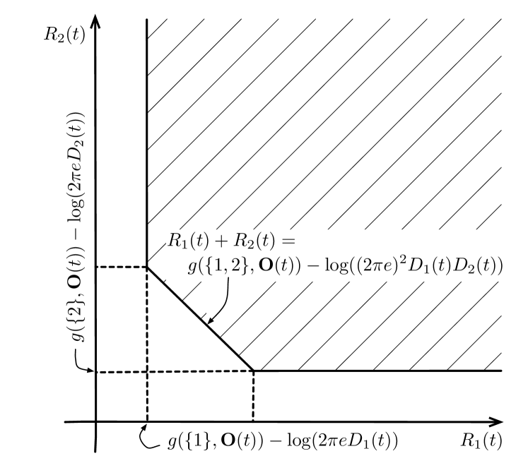
Figure 2: Illustration of the rate region (8) for correlated sources and ${\mathcal{N}}=\{1,2\}$. For all rate pairs $(R_{1}(t),R_{2}(t))$, there exists a coding schemes that enables the sink to recover the two sources with distributed distortion (MSE) levels $D_{1}(t)$ and $D_{2}(t)$, respectively.

To elaborate on this point, consider the following conditions on the rates $R_{n}(t)$ and distortions $D_{n}(t)$ for $n\in{\mathcal{N}}$:

$$\sum_{n\in{\mathcal{X}}}R_{n}(t)\geq{\mathrm{g}}({\mathcal{X}},{\textbf{O}}(t))-\log\left((2\pi e)^{|{\mathcal{X}}|}\prod_{n\in{\mathcal{X}}}D_{n}(t)\right),$$ (8)

for all ${\mathcal{X}}\subseteq{\mathcal{N}}$, where ${\mathrm{g}}({\mathcal{X}},{\textbf{O}}(t))$ denotes the joint conditional differential entropy of the sources measured by the nodes in the subset ${\mathcal{X}}$, where conditioning is with respect to the sources measured by the nodes in the complement ${\mathcal{N}}\setminus{\mathcal{X}}$. For instance, for jointly Gaussian sources with zero mean and correlation matrix ${\textbf{O}}(t)$, we have

$${\mathrm{g}}({\mathcal{X}},{\textbf{O}}(t))=\frac{1}{2}\log\left(\frac{\det{\textbf{O}}(t)}{\det{\textbf{O}}(t)|_{{\mathcal{N}}\setminus{\mathcal{X}}}}\right),$$ (9)

where ${\textbf{O}}(t)|_{{\mathcal{N}}\setminus{\mathcal{X}}}$ represents the correlation submatrix of the sources measured by nodes in ${\mathcal{N}}\setminus{\mathcal{X}}$. If the rates satisfy conditions (8), it is known [Zamir99] that, for sufficiently small distortions and any well-behaved joint source distribution, the sink is able to recover all the sources within MSE levels $D_{n}(t)$ for all $n\in{\mathcal{N}}$. We remark that this conclusion is also valid for any distortion tuple ${\mathbf{D}}(t)$ if the sources are jointly Gaussian.

As an example, the rate region for ${\mathcal{N}}=\{1,2\}$ is sketched in Fig. 2. The rates $R_{1}(t)$ and $R_{2}(t)$ at which the two source sequences are acquired and compressed at the two nodes can be traded with one another without affecting the distortions of the reconstructions at the sink, as long as they remain in the shown rate region (8).

We account for the cost of source acquisition and compression by defining a function ${P^{c}_{n}}(R_{n}(t))$ that provides the power spent for compressing the acquired data at a particular rate $R_{n}(t)$. For the sake of analytical tractability, we assume that each function ${P^{c}_{n}}(R_{n}(t))$ is

$${P^{c}_{n}}(R_{n}(t))=\alpha_{n}R_{n}(t),$$ (10)

for some coefficient $\alpha_{n}\geq 0$. Finally, we remark that the destination $d$ is assumed not to have sensing capabilities, and thus is not able to acquire any measurements. We will treat the extension to this setting in Section LABEL:sec:side_information.

II-C Energy Model

Every node in the network is assumed to be powered via energy harvesting. The harvested energy is stored in an energy storage device, or battery, which is modeled as an energy queue, as in e.g., [Huang10]. The energy queue size $E_{n}(t)$ at a node $n\in{\mathcal{N}}$ measures the amount of energy left in the battery of a node $n$ at the beginning of time slot $t$. For convenience, we normalize the available energy to the number of channel uses (transmission symbols) per slot. Without loss of generality, we assume unitary slot duration so that the amount of power consumed for transmission and acquisition/compression is equivalent to the energy spent in a time slot. Therefore, at any time slot $t$, the overall energy used at a node $n\in{\mathcal{N}}$ must satisfy the availability constraint

$$P_{n}+{P^{c}_{n}}(R_{n}(t))\leq E_{n}(t).$$ (11)

That is, the total consumed energy due to transmission and acquisition/compression must not exceed the energy available at the node.

We denote by $H_{n}(t)\leq{H_{\rm max}}$ the amount of energy harvestable by node $n$ at time slot $t$, and we define the vector ${\mathbf{H}}(t)=(H_{1}(t),\ldots,H_{N}(t))$ as the energy-harvesting state. We assume that ${\mathbf{H}}(t)$ takes value in a finite set ${\mathcal{H}}=\{{\mathbf{h}}_{1},{\mathbf{h}}_{2},\ldots,{\mathbf{h}}_{P}\}$, and is constant for the duration of a time slot, but i.i.d. over time slots. Finally, we define the probability $\rho_{{\mathbf{h}}_{i}}=\Pr[{\mathbf{H}}(t)={\mathbf{h}}_{i}]$, which accounts for possible spatial correlation of the harvestable energy across different nodes.

The energy harvested at time $t$ is assumed to be available for use at time $t+1$. Moreover, each node $n\in{\mathcal{N}}$ can decide how much of the harvestable energy $H_{n}(t)$ to store in the battery at time slot $t$, and we denote the harvesting decision by ${\widetilde{H}}_{n}(t)$, with $0\leq{\widetilde{H}}_{n}(t)\leq H_{n}(t)$. We define the harvesting decision vector as ${\widetilde{\mathbf{H}}}(t)=({\widetilde{H}}_{1}(t),\ldots,{\widetilde{H}}_{N}(t))$. Variable ${\widetilde{H}}_{n}(t)$ is introduced, following [Huang10], to address the issue of assessing the needs of the system in terms of capacities of the energy storage devices. In fact, as in [Huang10], we do not make any assumption about the battery maximum size. However, it will be proved later that performance arbitrarily close to the optimal attainable with no limitations on the battery capacity can be achieved with finite-capacity batteries.

II-D Queueing Dynamics

We now detail the dynamics of the network queues. We define ${\mathbf{E}}(t)=(E_{1}(t),\ldots,E_{N}(t))$ to be the vector of the energy queue sizes of all nodes at time $t$. From the discussion above, for each node $n\in{\mathcal{N}}$, $E_{n}(t)$ evolves as

$$E_{n}(t+1)=E_{n}(t)-P_{n}(t)-{P^{c}_{n}}(R_{n}(t))+{\widetilde{H}}_{n}(t),$$ (12)

since at each time slot $t$, the energy $P_{n}(t)+{P^{c}_{n}}(R_{n}(t))$ is consumed, while energy ${\widetilde{H}}_{n}(t)$ is harvested. We assume $E_{n}(0)\geq 0$ for all $n\in{\mathcal{N}}$.

We also define the vector ${\mathbf{U}}(t)=(U_{1}(t),\ldots,U_{N}(t))$, for each time slot $t$, to be the network data queue backlog, where $U_{n}(t)$ represents the amount of data queued at node $n$, which is normalized on the number of channel uses per time slot for convenience of notation, that is it is expressed in terms of bits over channel uses per slot. Denote as $b$ the ratio between the number of channel uses per slot and the number of source samples per slot. Since $b$ typically accounts for the ratio of the channel and source bandwidth, it is conventionally referred to as bandwidth ratio, [ElGamal12]. We assume that each queue $U_{n}(t)$ evolves according to the following dynamics:

$$U_{n}(t+1)\leq\max\left\{U_{n}(t)-{\mu_{n,*}}(t),0\right\}+{\mu_{*,n}}(t)+\frac{R_{n}(t)}{b},$$ (13)

since at any time slot $t$, each node $n\in{\mathcal{N}}$ can transmit, and thus remove from its data queue, at most ${\mu_{n,*}}(t)$ bits per channel use, while it can receive at most ${\mu_{*,n}}(t)$ bits per channel use due to transmissions from other nodes and $R_{n}(t)/b$ bits per channel use due to data acquisition/compression. We assume that $U_{n}(0)=0$ for all $n\in{\mathcal{N}}$. Following standard definitions [Neely10], we say that the network is stable if the following condition holds true:

$${\underset{T\to\infty}{\lim\!\sup\ }}\frac{1}{T}\sum_{t=0}^{T-1}\sum_{n\in{\mathcal{N}}}{\mathbb{E}}[U_{n}(t)]<\infty.$$ (14)

Notice that the network stability condition (14) implies that the data queue $U_{n}(t)$ of each node $n\in{\mathcal{N}}$ is stable in the sense that ${\underset{T\to\infty}{\lim\!\sup\ }}\frac{1}{T}\sum_{t=0}^{T-1}{\mathbb{E}}[U_{n}(t)]<\infty$.

$${\mathrm{d}}_{{\textbf{o}}_{i},{\textbf{s}}_{j},{\mathbf{h}}_{k}}({\bm{\lambda}}^{({\textbf{o}}_{i})},{\bm{\upsilon}},{\bm{\chi}})=\inf_{{\mathbf{R}}^{({\textbf{o}}_{i})},{\mathbf{D}}^{({\textbf{o}}_{i})},{\mathbf{P}}^{({\textbf{s}}_{j})},{\widetilde{\mathbf{H}}}^{({\mathbf{h}}_{k})}}\Bigg{\{}\sum_{n\in{\mathcal{N}}}V{\mathrm{f}_{n}}(D_{n}^{({\textbf{o}}_{i})})+\sum_{m=1}^{2^{N}-1}\lambda_{m}^{({\textbf{o}}_{i})}\Bigg{[}{\mathrm{g}}({\mathcal{X}}_{m},{\textbf{o}}_{i})-\log\left((2\pi e)^{|{\mathcal{X}}_{m}|}\prod_{n\in{\mathcal{X}}_{m}}D_{n}^{({\textbf{o}}_{i})}\right)$$

$$\;\;\;\;\;\;-\sum_{n\in{\mathcal{X}}_{m}}R_{n}^{({\textbf{o}}_{i})}\Bigg{]}+\sum_{n\in{\mathcal{N}}}\upsilon_{n}\Bigg{[}\frac{R_{n}^{({\textbf{o}}_{i})}}{b}+{\mu_{*,n}}({\mathbf{P}}^{({\textbf{s}}_{j})},{\textbf{s}}_{j})-{\mu_{n,*}}({\mathbf{P}}^{({\textbf{s}}_{j})},{\textbf{s}}_{j})\Bigg{]}+\sum_{n\in{\mathcal{N}}}\chi_{n}\left[P_{n}^{({\textbf{s}}_{j})}+{P^{c}_{n}}(R_{n}^{({\textbf{o}}_{i})})-{\widetilde{H}}_{n}^{({\mathbf{h}}_{k})}\right]\Bigg{\}}$$ (19)

II-E Optimization Problem

Define $\Theta(t)=\left({\textbf{S}}(t),{\textbf{O}}(t),{\mathbf{H}}(t),{\mathbf{U}}(t),{\mathbf{E}}(t)\right)$ as the state of the network at time slot $t$. A (past-dependent) policy $\pi=\{\pi(t)\text{: }t=1,2,\ldots\}$ is a collection of mappings between the past and current states $\{\Theta(\tau)\text{: }\tau=1,\ldots,t\}$ and the current decision $({\mathbf{R}}(t),{\mathbf{D}}(t),{\widetilde{\mathbf{H}}}(t),{\mathbf{P}}(t))$ on rates ${\mathbf{R}}(t)$, distortion levels ${\mathbf{D}}(t)$, harvested energy ${\widetilde{\mathbf{H}}}(t)$ and transmission powers ${\mathbf{P}}(t)$. Moreover, for each node $n\in{\mathcal{N}}$, let ${\mathrm{f}_{n}}(D_{n}(t))$ denote the cost incurred by node $n$ when its corresponding distortion is $D_{n}(t)$. We assume that each function ${\mathrm{f}_{n}}(D_{n}(t))$ is convex, finite and non-decreasing in the interval $[{D_{\rm min}},{D_{\rm max}}]$. Our objective is to solve the following optimization problem:

$$\underset{\pi}{\operatorname{minimize}}\ F_{0}^{\pi}=\sum_{n\in{\mathcal{N}}}F_{n}^{\pi}$$ (15)

where

$$F_{n}^{\pi}={{\underset{T\to\infty}{\lim\!\sup\ }}\frac{1}{T}\sum_{t=0}^{T-1}{\mathbb{E}}[{\mathrm{f}_{n}}(D_{n}(t))]},$$ (16)

subject to the rate-distortion constraints (8), the energy availability constraint (11) and network stability constraint (14). Note that (16) is the per-slot average cost for node $n$.

III Lower bound

In this section, we obtain a lower bound on the optimal network cost $F_{0}^{*}$ of problem (15). This result will be used in Section LABEL:sec:performance to obtain analytical performance guarantees on our online optimization policy, presented in Section IV. The lower bound is expressed in terms of an optimization problem over parameters ${\mathbf{R}}^{({\textbf{o}}_{i})}=[R_{1}^{({\textbf{o}}_{i})},\ldots,R_{N}^{({\textbf{o}}_{i})}]$ and ${\mathbf{D}}^{({\textbf{o}}_{i})}=[D_{1}^{({\textbf{o}}_{i})},\ldots,D_{N}^{({\textbf{o}}_{i})}]$ for all ${\textbf{o}}_{i}\in{\mathcal{O}}$, ${\mathbf{P}}^{({\textbf{s}}_{j})}$ with entries $P_{n,m}^{({\textbf{s}}_{j})}$ for each $(n,m)\in{\mathcal{L}}$ and for all ${\textbf{s}}_{j}\in{\mathcal{S}}$, and ${\widetilde{\mathbf{H}}}^{({\mathbf{h}}_{k})}=[{\widetilde{H}}_{1}^{({\mathbf{h}}_{k})},\ldots,{\widetilde{H}}_{N}^{({\mathbf{h}}_{k})}]$ for all ${\mathbf{h}}_{k}\in{\mathcal{H}}$. The proof is based on relaxing the stability constraint (14) by imposing the necessary condition that the average arrival rate at each data queue be smaller than or equal to the average departure rate, and by also relaxing the energy availability constraint (11) by requiring it to be satisfied only on average. Finally, Lagrange relaxation is used on the resulting problem. The details of the proof are available in Appendix LABEL:sec:proof_thm:optimal.

Theorem III.1

The optimal network cost $F_{0}^{*}$ satisfies the following inequality:

$$VF_{0}^{*}\geq{\mathrm{d}}({\bm{\lambda}},{\bm{\upsilon}},{\bm{\chi}}),$$ (17)

for all ${\bm{\lambda}}\in\mathbb{R}^{L(2^{N}-1)}_{+},{\bm{\upsilon}}\in\mathbb{R}^{N}_{+},{\bm{\chi}}\in\mathbb{R}^{N}$, where ${\mathrm{d}}({\bm{\lambda}},{\bm{\upsilon}},{\bm{\chi}})$ is given by

$$\begin{split}{\mathrm{d}}({\bm{\lambda}},&{\bm{\upsilon}},{\bm{\chi}})=\sum_{{\textbf{o}}_{i}\in{\mathcal{O}}}\rho_{{\textbf{o}}_{i}}\!\sum_{{\textbf{s}}_{j}\in{\mathcal{S}}}\!\rho_{{\textbf{s}}_{j}}\!\sum_{{\mathbf{h}}_{k}\in{\mathcal{H}}}\!\rho_{{\mathbf{h}}_{k}}d_{{\textbf{o}}_{i},{\textbf{s}}_{j},{\mathbf{h}}_{k}}({\bm{\lambda}}^{({\textbf{o}}_{i})},{\bm{\upsilon}},{\bm{\chi}}),\end{split}$$ (18)

with $d_{{\textbf{o}}_{i},{\textbf{s}}_{j},{\mathbf{h}}_{k}}({\bm{\lambda}}^{({\textbf{o}}_{i})},{\bm{\upsilon}},{\bm{\chi}})$ defined in (II-D), where the infimum is taken under constraints:

$$\begin{split}0\leq R_{n}^{({\textbf{o}}_{i})}\leq{R_{\rm max}},&{D_{\rm min}}\leq D_{n}^{({\textbf{o}}_{i})}\leq{D_{\rm max}},\\ &\text{for all }n\in{\mathcal{N}},{\textbf{o}}_{i}\in{\mathcal{O}},\end{split}$$ (20)

$$0\leq P_{n}^{({\textbf{s}}_{j})}\leq{P_{\rm max}},\text{for all }n\in{\mathcal{N}},{\textbf{s}}_{j}\in{\mathcal{S}},$$ (21)

$$\text{and }0\leq{\widetilde{H}}_{n}^{({\mathbf{h}}_{k})}\leq{\mathbf{h}}_{k,n},\text{for all }n\in{\mathcal{N}},{\mathbf{h}}_{k}\in{\mathcal{H}}.$$ (22)

Proof:

See Appendix LABEL:sec:proof_thm:optimal. ∎

IV Proposed Policy

In this section, we propose an algorithm designed following the Lyapunov optimization framework, as developed in [Georgiadis06] [Neely10], to solve the optimization problem (15). In particular, we aim at finding an online policy $\pi$ for problem (15) with close-to-optimal performance, by using Lyapunov optimization with weight perturbation. The technique of weight perturbation, as proposed in [Huang10], is used to ensure that the energy queues are kept close to a target value. This is done to avoid battery underflow in a way that is reminiscent of the battery management strategies put forth in [Srivastava10], and is further discussed below.

The proposed policy operates by approximately minimizing at each time slot the one-slot conditional Lyapunov drift plus penalty [Neely10] of the energy and data queues ((12) and (13), respectively) of the network. The optimization is done in an on-line fashion based on the knowledge of the current channel state ${\textbf{S}}(t)$, observation state ${\textbf{O}}(t)$, data queue sizes ${\mathbf{U}}(t)$ and energy queue sizes ${\mathbf{E}}(t)$. Note that no knowledge of the statistics of the states is required, as it is standard with Lyapunov optimization techniques [Georgiadis06, Neely10]. Using this approach, we obtained the following online optimization algorithm.

Algorithm: Fix a weight ${\boldsymbol{\theta}}=[\theta_{1},\ldots,\theta_{N}]\in\mathbb{R}^{N}_{+}$ and a parameter $V>0$. At each time slot $t$, based on the values of the queues ${\mathbf{E}}(t)$ and ${\mathbf{U}}(t)$, channel states ${\textbf{S}}(t)$ and observation states ${\textbf{O}}(t)$, perform the following:

• Energy Harvesting: For each node $n\in{\mathcal{N}}$, choose ${\widetilde{H}}_{n}(t)$ that minimizes $(E_{n}(t)-\theta_{n}){\widetilde{H}}_{n}(t)$ under the constraint $0\leq{\widetilde{H}}_{n}(t)\leq H_{n}(t)$. That is, if $(E_{n}(t)-\theta_{n})<0$, perform energy harvesting and store the harvested energy, i.e., set ${\widetilde{H}}_{n}(t)=\min\{\theta_{n}-E_{n}(t),H_{n}(t)\}$; otherwise, perform no harvesting, i.e., set ${\widetilde{H}}_{n}(t)=0$;

• Rate-Distortion Optimization: Choose the source acquisition/compression rate vector ${\mathbf{R}}(t)={\mathbf{r}}=[r_{1},\ldots,r_{N}]$ and the distortion levels ${\mathbf{D}}(t)={\mathbf{d}}=[d_{1},\ldots,d_{N}]$ to be an optimal solution of the following optimization problem:

  $$\begin{split}\underset{{\mathbf{r}},{\mathbf{d}}}{\operatorname{minimize\ }}\sum_{n\in{\mathcal{N}}}[U_{n}(t)r_{n}-(E_{n}(t)-\theta_{n}){P^{c}_{n}}(r_{n})\\ +V{\mathrm{f}_{n}}(d_{n})],\end{split}$$ (23)

  subject to the rate-distortion region constraint (8), and to the constraints $0\leq r_{n}\leq{R_{\rm max}}$ and ${D_{\rm min}}\leq d_{n}\leq{D_{\rm max}}$, for all $n\in{\mathcal{N}}$;

• Power Allocation: Define the weight of a link $(n,m)$ as

  $$W_{n,m}(t)=\max\{U_{n}(t)-U_{m}(t)-\delta,0\},$$ (24)

  where $\delta={l_{\rm max}}{\mu_{\rm max}}+{R_{\rm max}}$, and choose ${\mathbf{P}}(t)={\mathbf{p}}$ with entries $p_{n,m}$ for $(n,m)\in{\mathcal{L}}$ to be an optimal solution of the following optimization problem:

  $$\begin{split}\underset{{\mathbf{p}}}{\operatorname{maximize\ }}\sum_{n\in{\mathcal{N}}}\Big{[}\sum_{m\in{\mathcal{N}}\setminus n}{\mathrm{C}}_{n,m}({\mathbf{p}},{\textbf{S}}(t))W_{n,m}(t)\\ +(E_{n}(t)-\theta_{n})p_{n}\Big{]},\end{split}$$ (25)

  where $p_{n}=\sum_{m\in{\mathcal{N}}\setminus n}p_{n,m}$, subject to constraints $0\leq p_{n}\leq{P_{\rm max}}$, for each $n\in{\mathcal{N}}$;

• Queues Update: Update ${\mathbf{E}}(t)$ and ${\mathbf{U}}(t)$ according to (12) and (13), respectively.