Methodology of Numerical Computations
with Infinities and Infinitesimals

Abstract

A recently developed computational methodology for executing numerical calculations with infinities and infinitesimals is described in this paper. The developed approach has a pronounced applied character and is based on the principle ‘The part is less than the whole’ introduced by Ancient Greeks. This principle is used with respect to all numbers (finite, infinite, and infinitesimal) and to all sets and processes (finite and infinite). The point of view on infinities and infinitesimals (and in general, on Mathematics) presented in this paper uses strongly physical ideas emphasizing interrelations holding between a mathematical object under the observation and tools used for this observation. It is shown how a new numeral system allowing one to express different infinite and infinitesimal quantities in a unique framework can be used for theoretical and computational purposes. Numerous examples dealing with infinite sets, divergent series, limits, and probability theory are given.

AMS Subject Classification: 03E65, 65-02, 65B10, 60A10

1 Introduction

The concept of infinity attracted the attention of people during millenniums (see monographs [1, 4, 6, 9, 10, 12, 13, 14, 16] and references given therein). To emphasize importance of the subject for modern Mathematics it is sufficient to mention that the Continuum Hypothesis related to infinity has been included by David Hilbert as the Problem Number One in his famous list of 23 unsolved mathematical problems (see [10]) that have influenced strongly development of Mathematics in the XX-th century.

There exist different ways to generalize traditional arithmetic for finite numbers to the case of infinities and infinitesimals (see, e.g., [1, 4, 16] and references given therein). However, the arithmetics developed for infinite numbers up to now were quite different with respect to the finite arithmetic we are used to deal with. Very often they leave undetermined many operations where infinity takes part (for example, $\infty-\infty$, $\frac{\infty}{\infty}$, sum of infinitely many items, etc.) or use a representation of infinite numbers based on infinite sequences of finite numbers. In spite of these crucial difficulties and due to enormous importance of the concept of infinity in science, people try to introduce infinity in their work with computers. We can mention the IEEE Standard for Binary Floating-Point Arithmetic containing representations for $+\infty$ and $-\infty$ and incorporation of these notions in the interval analysis implementations.

The development of the modern views on infinity and infinitesimals strangely enough was not simultaneous. The point of view on infinity accepted nowadays takes its origins from the famous ideas of Georg Cantor (see [1]) who has shown that there exist infinite sets having different cardinalities. On the other hand, in the early history of Calculus, arguments involving infinitesimals played a pivotal role in the differential Calculus developed by Leibniz and Newton (see [12, 14]). The notion of an infinitesimal, however, lacked a precise mathematical definition and, in order to provide a more rigorous foundation for the Calculus, infinitesimals were gradually replaced by the d’Alembert–Cauchy concept of a limit (see [3, 5]).

The creation of a rigorous mathematical theory of infinitesimals remained an open problem until the end of the 1950s when Robinson (see [16]) has introduced his famous non-standard Analysis approach. He has shown that non-archimedean ordered field extensions of the reals contained numbers that could serve the role of infinitesimals and their reciprocals could serve as infinitely large numbers. Robinson then has derived the theory of limits, and more generally of Calculus, and has found a number of important applications of his ideas in many other fields of Mathematics (see [16]).

In his approach, Robinson used mathematical tools and terminology (cardinal numbers, countable sets, continuum, one-to-one correspondence, etc.) taking their origins from the ideas of Cantor (see [1]) introducing so all advantages and disadvantages of Cantor’s theory in non-standard Analysis, as well. In fact, it is well known nowadays that while dealing with infinite sets, Cantor’s approach leads to some counterintuitive situations that often are called by non-mathematicians as ‘paradoxes’. For example, the set of even numbers, $\mathbb{E}$, can be put in a one-to-one correspondence with the set of all natural numbers, $\mathbb{N}$, in spite of the fact that $\mathbb{E}$ is a proper subset of $\mathbb{N}$:

$$\begin{array}[]{lccccccc}\mbox{even numbers:}&\hskip 14.22636pt2,&4,&6,&8,&10,&12,&\ldots\\ &\hskip 14.22636pt\updownarrow&\updownarrow&\updownarrow&\updownarrow&\updownarrow&\updownarrow&\\ \mbox{natural numbers:}&\hskip 14.22636pt1,&2,&3,&4&5,&6,&\ldots\\ \end{array}$$ (1)

In contrast, we can observe that for finite sets, if a set $A$ is a proper subset of a set $B$ then it follows that the number of elements of the set $A$ is smaller than the number of elements of the set $B$.

Another famous example that is difficult for understanding for many people is Hilbert’s paradox of the Grand Hotel having the following formulation. In a normal hotel with a finite number of rooms no more new guests can be accommodated if it is full. Hilbert’s Grand Hotel has an infinite number of rooms (of course, the number of rooms is countable, because the rooms in the Hotel are numbered). Due to Cantor, if a new guest arrives at the Hotel where every room is occupied, it is, nevertheless, possible to find a room for him. To do so, it is necessary to move the guest occupying room 1 to room 2, the guest occupying room 2 to room 3, etc. In such a way room 1 will be ready for the newcomer and, in spite of our assumption that there are no available rooms in the Hotel, we have found one.

These results are very difficult to be fully realized by anyone who is not a mathematician since in our every day experience in the world around us the part is always less than the whole and if a hotel is complete there are no places in it. In order to understand how it is possible to tackle the situations discussed above in accordance with the principle ‘the part is less than the whole’ let us consider a study published in Science (see [8]) where the author describes a primitive tribe living in Amazonia - Pirahã - that uses a very simple numeral system for counting: one, two, many. For Pirahã, all quantities larger than two are just ‘many’ and such operations as 2+2 and 2+1 give the same result, i.e., ‘many’. Using their weak numeral system Pirahã are not able to see, for instance, numbers 3, 4, 5, and 6, to execute arithmetical operations with them, and, in general, to say anything about these numbers because in their language there are neither words nor concepts for that. Moreover, the weakness of Pirahã’s numeral system leads to such results as

$$\mbox{`many'}+1=\mbox{`many'},\hskip 28.45274pt\mbox{`many'}+2=\mbox{`many'},$$

which are very familiar to us in the context of views on infinity used in the traditional calculus

$$\infty+1=\infty,\hskip 28.45274pt\infty+2=\infty.$$

Thus, the modern mathematical numeral systems allow us to distinguish a larger quantity of finite numbers with respect to Pirahã but give similar results when we speak about infinite numbers.

The arithmetic of Pirahã involving the numeral ‘many’ has also a clear similarity with the arithmetic proposed by Cantor for his Alephs. This similarity becomes even stronger if one considers another Amazonian tribe – Mundurukú (see [15]) – who fail in exact arithmetic with numbers larger than 5 but are able to compare and add large approximate numbers that are far beyond their naming range. Particularly, they use the words ‘some, not many’ and ‘many, really many’ to distinguish two types of large numbers (in this connection think about Cantor’s $\aleph_{0}$ and $\aleph_{1}$).

These observations lead us to the following idea: Probably our difficulty in working with infinity is not connected to the nature of infinity but is a result of inadequate numeral systems used to express infinite numbers. Analogously, Pirahã are not able to distinguish numbers 3 and 4 not due to the nature of these numbers but due to the weakness of the numeral system that Pirahã use.

In this paper, we show how the introduction of a new numeral allows one to express different infinite and infinitesimal quantities. Taken together with a new (physically oriented) methodology for Mathematics, the new numeral system can be used for theoretical and computational purposes using the Infinity Computer (see [24]) able to work numerically with infinite and infinitesimal numbers expressed in the new numeral system.

2 From absolute mathematical truths to their relativity and accuracy of mathematical results

In this section, we give a brief introduction to the new methodology that can be found in a rather comprehensive form in the survey [20] downloadable from [27] (see also the monograph [18] written in a popular manner and [22] describing the foundations of a new differential calculus). Numerous examples of the usage of the proposed methodology can be found in [18, 19, 21, 23, 25, 26, 27]. The goal of the entire operation is to propose a way of thinking that would allow us to work with finite, infinite, and infinitesimal numbers in the same way, namely, in the way we are used to deal with finite quantities in the world around us.

In order to start, let us make some observations. As was mentioned above, foundations of the modern Set Theory dealing with infinity have been developed starting from the end of the XIX-th century until more or less the first decades of the XX-th century. Foundations of the classical Analysis dealing both with infinity and infinitesimals have been developed even earlier, more than 200 years ago. The goal of its creation was to produce mathematical tools allowing one to solve problems arising in the real world in that time. As a result, classical Analysis was build using the common in that time background of ideas that people had about Physics (and Philosophy). Thus, these parts of Mathematics do not include numerous achievements of Physics of the XX-th century. In fact, the classical Analysis operates with absolute truths and ideas of relativity and quants are not reflected in it. Let us give just one example to clarify this point.

In modern Physics, the ‘continuity’ of an object is relative. If we observe a table by eye, then we see it as being continuous. If we use a microscope for our observation, we see that the table is discrete. This means that we decide how to see the object, as a continuous or as a discrete, by the choice of the instrument for the observation. A weak instrument – our eyes – is not able to distinguish its internal small separate parts (e.g., molecules) and we see the table as a continuous object. A sufficiently strong microscope allows us to see the separate parts and the table becomes discrete but each small part now is viewed as continuous.

In contrast, in traditional Mathematics, any mathematical object is either continuous or discrete. For example, the same function cannot be both continuous and discrete. Thus, this contraposition of discrete and continuous in the traditional Mathematics does not reflect properly the physical situation that we observe in practice.

Note that even results of Robinson made in the middle of the XX-th century have been also directed to a reformulation of the classical Analysis in terms of infinitesimals and not to the creation of a new kind of Analysis that would incorporate new achievements of Physics. In fact, he wrote in paragraph 1.1 of his famous book [16]: ‘It is shown in this book that Leibniz’ ideas can be fully vindicated and that they lead to a novel and fruitful approach to classical Analysis and to many other branches of mathematics’.

In order to overcome this delay with the introduction of ideas of Physics of the XX-th century in Mathematics, the point of view on infinities and infinitesimals (and in general, on Mathematics) presented in this paper uses strongly relativity and interrelations holding between the object of an observation and the tool used for this observation. The latter is directly related to connections between numeral systems used to describe mathematical objects and the objects themselves. Numerals that we use to write down numbers, functions, etc. are among our tools of the investigation and, as a result, they strongly influence our capabilities to study mathematical objects.

This separation (having an evident physical spirit) of mathematical objects from tools used for their description is crucial for our study but it is used rarely in contemporary Mathematics. In fact, the idea of finding an adequate (absolutely the best) set of axioms for one or another field of Mathematics continues to be among the most attractive goals for contemporary mathematicians. Usually, when it is necessary to define a concept or an object, logicians try to introduce a number of axioms defining the object. However, this way is fraught with danger because of the following reasons.

First, when we describe a mathematical object or concept we are limited by the expressive capacity of the language we use to make this description. A richer language allows us to say more about the object and a weaker language – less. Thus, development of the mathematical (and not only mathematical) languages leads to a continuous necessity of a transcription and specification of axiomatic systems. Second, there is no guarantee that the chosen axiomatic system defines ‘sufficiently well’ the required concept and a continuous comparison with practice is required in order to check the goodness of the accepted set of axioms. However, there cannot be again any guarantee that the new version will be the last and definitive one. Finally, the third limitation already mentioned above has been discovered by Gödel in his two famous incompleteness theorems (see [7]).

It should be emphasized that in Linguistics, the relativity of the language with respect to the world around is a well known thing. It has been formulated in the form of the Sapir–Whorf thesis (see [2, 17]) also known as the ‘linguistic relativity thesis’. As becomes clear from its name, the thesis does not accept the idea of the universality of language and postulates that the nature of a particular language influences the thought of its speakers. The thesis challenges the possibility of perfectly representing the world with language, because it implies that the mechanisms of any language condition the thoughts of its speakers.

Thus, our point of view on axiomatic systems is different. It is significantly more applied and less ambitious and is related only to utilitarian necessities to make calculations. In contrast to the modern mathematical fashion that tries to make all axiomatic systems more and more precise (decreasing so degrees of freedom of the studied part of Mathematics), we just define a set of general rules describing how practical computations should be executed leaving so as much space as possible for further, dictated by practice, changes and developments of the introduced mathematical language. Speaking metaphorically, we prefer to make a hammer and to use it instead of describing what is a hammer and how it works.

Since our point of view on the mathematical world is significantly more physical and more applied than the traditional one, it becomes necessary to clarify it better. Let us formulate three methodological postulates that will guide our further study and will show where our positions are different with respect to the tradition.

Traditionally, when mathematicians deal with infinite objects (sets or processes) it is supposed that human beings are able to execute certain operations infinitely many times (e.g., see (1)). However, since we live in a finite world and all human beings and/or computers are forced to finish operations that they have started, this supposition is not adopted.

Postulate 1. There exist infinite and infinitesimal objects but human beings and machines are able to execute only a finite number of operations.

Due to this Postulate, we accept a priori that we shall never be able to give a complete description of infinite processes and sets due to our finite capabilities.

The second postulate is adopted following the way of reasoning used in natural sciences where researchers use tools to describe the object of their study and the used instrument influences the results of the observations. When a physicist uses a weak lens $A$ and sees two black dots in his/her microscope he/she does not say: The object of the observation is two black dots. The physicist is obliged to say: the lens used in the microscope allows us to see two black dots and it is not possible to say anything more about the nature of the object of the observation until we change the instrument - the lens or the microscope itself - by a more precise one. Suppose that he/she changes the lens and uses a stronger lens $B$ and is able to observe that the object of the observation is viewed as ten (smaller) black dots. Thus, we have two different answers: (i) the object is viewed as two dots if the lens $A$ is used; (ii) the object is viewed as ten dots by applying the lens $B$. Which of the answers is correct? Both. Both answers are correct but with the different accuracies that depend on the lens used for the observation.

The same happens in Mathematics studying natural phenomena, numbers, and objects that can be constructed by using numbers. Numeral systems used to express numbers are among the instruments of observations used by mathematicians. The usage of powerful numeral systems gives the possibility to obtain more precise results in Mathematics in the same way as usage of a good microscope gives the possibility of obtaining more precise results in Physics. However, the capabilities of the tools will be always limited due to Postulate 1 (we are able to write down only a finite number of symbols when we wish to describe a mathematical object) and due to Postulate 2 we shall never tell, what is, for example, a number but shall just observe it through numerals expressible in a chosen numeral system.

Postulate 2. We shall not tell what are the mathematical objects we deal with; we just shall construct more powerful tools that will allow us to improve our capacities to observe and to describe properties of mathematical objects.

This means that mathematical results are not absolute, they depend on mathematical languages used to formulate them, i.e., there always exists an accuracy of the description of a mathematical result, fact, object, etc. For instance, the result of Pirahã $2+2=$ ‘many’ is not wrong, it is just inaccurate. The introduction of a stronger tool (in this case, a numeral system that contains a numeral for a representation of the number four) allows us to have a more precise answer.

It is necessary to comment upon another important aspect of the distinction between a mathematical object and a mathematical tool used to observe this object. The Postulates 1 and 2 impose us to think always about the possibility to execute a mathematical operation by applying a numeral system. They tell us that there always exist situations where we are not able to express the result of an operation. Let us consider, for example, the operation of construction of the successive element widely used in number and set theories. In the traditional Mathematics, the aspect whether this operation can be executed is not taken into consideration, it is supposed that it is always possible to execute the operation $k=n+1$ starting from any integer $n$. Thus, there is no any distinction between the existence of the number $k$ and the possibility to execute the operation $n+1$ and to express its result, i.e. to have a numeral that can express $k$.

Postulates 1 and 2 emphasize this distinction and tell us that: (i)  in order to execute the operation it is necessary to have a numeral system allowing one to express both numbers, $n$ and $k$; (ii) for any numeral system there always exists a number $k$ that cannot be expressed in it. For instance, for Pirahã $k=3$, for Mundurukú $k=6$. Even for modern powerful numeral systems there exist such a number $k$ (for instance, nobody is able to write down a numeral in the decimal positional system having $10^{100}$ digits). Hereinafter we shall always emphasize the triad – researcher, object of the investigation, and tools used to observe the object – in various mathematical and computational contexts paying a special attention to the accuracy of the obtained results.

Particularly, Postulate 2 means that, from our point of view, axiomatic systems do not define mathematical objects but just determine formal rules for operating with certain numerals reflecting some properties of the studied mathematical objects using a certain mathematical language $L$. We are aware that the chosen language $L$ has its accuracy and there always can exist a richer language $\tilde{L}$ that would allow us to describe the studied object better. Due to Postulate 1, any language has a limited expressibility, in particular, there always exist situations where the accuracy of the answers expressible in this language is not sufficient. Such situations lead to ‘paradoxes’ showing the boundaries of the applicability of a language (theory, concept, etc.)

Let us return again to Pirahã and illustrate this point by using their answers $2+1=$ ‘many’ and $2+2=$ ‘many’. From these two identities one can obtain the result $2+1=2+2$ being a ‘paradox’. From our point of view, this situation just determines the boundaries of the applicability of their numeral system.

Finally, we adopt the principle of Greeks mentioned above as the third postulate.

Postulate 3. The principle ‘The part is less than the whole’ is applied to all numbers (finite, infinite, and infinitesimal) and to all sets and processes (finite and infinite).

Due to this declared applied statement, it becomes clear that the subject of this paper is out of Cantor’s approach and, as a consequence, out of non-standard Analysis of Robinson. Such concepts as bijection, numerable and continuum sets, cardinal and ordinal numbers cannot be used in this paper because they belong to the theory working with different assumptions. However, the approach used here does not contradict Cantor and Robinson. It can be viewed just as a more strong lens of a mathematical microscope that allows one to distinguish more objects and to work with them.

3 An infinite unit of measure expressible by a new numeral

In [18, 20], a new numeral system has been developed in accordance with methodological Postulates 1–3. It gives a possibility to execute numerical computations not only with finite numbers but also with infinite and infinitesimal ones. The main idea consists of the possibility to measure infinite and infinitesimal quantities by different (infinite, finite, and infinitesimal) units of measure.

A new infinite unit of measure has been introduced for this purpose as the number of elements of the set $\mathbb{N}$ of natural numbers. The new number is called grossone and is expressed by the numeral ①. It is necessary to stress immediately that ① is neither Cantor’s $\aleph_{0}$ nor $\omega$. Particularly, it has both cardinal and ordinal properties as usual finite natural numbers (see [20]). Note also that since ①, on the one hand, and $\aleph_{0}$ (and $\omega$), on the other hand, belong to different mathematical languages working with different theoretical assumptions, they cannot be used together. Analogously, it is not possible to use together Piraha’s ‘many’ and the modern numeral 4.

Formally, grossone is introduced as a new number by describing its properties postulated by the Infinite Unit Axiom (IUA) (see [18, 20]). This axiom is added to axioms for real numbers similarly to addition of the axiom determining zero to axioms of natural numbers when integer numbers are introduced. It is important to emphasize that we speak about axioms for real numbers in sense of Postulate 2, i.e., axioms do not define real numbers, they just define formal rules of operations with numerals in given numeral systems (tools of the observation) reflecting so certain (not all) properties of the object of the observation, i.e., properties of real numbers.

Inasmuch as it has been postulated that grossone is a number, all other axioms for numbers hold for it, too. Particularly, associative and commutative properties of multiplication and addition, distributive property of multiplication over addition, existence of inverse elements with respect to addition and multiplication hold for grossone as for finite numbers. This means that the following relations hold for grossone, as for any other number

$$0\cdot\hbox{$\displaystyle{\mbox{\char 172}}$}=\hbox{$\displaystyle{\mbox{\char 172}}$}\cdot 0=0,\hskip 8.53581pt\hbox{$\displaystyle{\mbox{\char 172}}$}-\hbox{$\displaystyle{\mbox{\char 172}}$}=0,\hskip 8.53581pt\frac{\hbox{$\displaystyle{\mbox{\char 172}}$}}{\hbox{$\displaystyle{\mbox{\char 172}}$}}=1,\hskip 8.53581pt\hbox{$\displaystyle{\mbox{\char 172}}$}^{0}=1,\hskip 8.53581pt1^{\mbox{\tiny{\hbox{$\displaystyle{\mbox{\char 172}}$}}}}=1,\hskip 8.53581pt0^{\mbox{\tiny{\hbox{$\displaystyle{\mbox{\char 172}}$}}}}=0.$$ (2)

The introduction of the new numeral allows us to use it for construction of various new numerals expressing infinite and infinitesimal numbers and to operate with them as with usual finite constants. As a consequence, the numeral $\infty$ is excluded from our new mathematical language (together with numerals $\aleph_{0},\aleph_{1},\ldots$ and $\omega$). In fact, since we are able now to express explicitly different infinite numbers, records of the type $\sum_{i=1}^{\infty}a_{i}$ become a kind of $\sum_{i=1}^{many}a_{i}$, i.e., they are not sufficiently precise. It becomes necessary not only to say that $i$ goes to infinity, it is necessary to indicate to which point in infinity (e.g., $\hbox{$\displaystyle{\mbox{\char 172}}$},5\hbox{$\displaystyle{\mbox{\char 172}}$}-1,\hbox{$\displaystyle{\mbox{\char 172}}$}^{2}+3$, etc.) we want to sum up. Note that for sums having a finite number of items the situation is the same: it is not sufficient to say that the number of items in the sum is finite, it is necessary to indicate explicitly the number of items in the sum.

The appearance of new numerals expressing infinite and infinitesimal numbers gives us a lot of new possibilities. For example, it becomes possible to develop a Differential Calculus (see [22]) for functions that can assume finite, infinite, and infinitesimal values and can be defined over finite, infinite, and infinitesimal domains avoiding indeterminate forms and divergences (all these concepts just do not appear in the new Calculus). This approach allows us to work with derivatives and integrals that can assume not only finite but infinite and infinitesimal values, as well. Infinite and infinitesimal numbers are not auxiliary entities in the new Calculus, they are full members in it and can be used in the same way as finite constants.

Let us comment upon the nature of grossone and give some examples illustrating its usage and, in particular, its direct links with infinite sets.

Example 3.1.

Grossone has been introduced as the number of elements of the set $\mathbb{N}$ of natural numbers. As a consequence, similarly to the set

$$A=\{1,2,3,4,5\}$$ (3)

consisting of 5 natural numbers where 5 is the largest number in $A$, ① is the largest number in $\mathbb{N}$ and $\hbox{$\displaystyle{\mbox{\char 172}}$}\in\mathbb{N}$ analogously to the fact that 5 belongs to $A$. Thus, the set, $\mathbb{N}$, of natural numbers can be written in the form

$$\mathbb{N}=\{1,2,\hskip 8.53581pt\ldots\hskip 8.53581pt\frac{\hbox{$\displaystyle{\mbox{\char 172}}$}}{2}-2,\frac{\hbox{$\displaystyle{\mbox{\char 172}}$}}{2}-1,\frac{\hbox{$\displaystyle{\mbox{\char 172}}$}}{2},\frac{\hbox{$\displaystyle{\mbox{\char 172}}$}}{2}+1,\frac{\hbox{$\displaystyle{\mbox{\char 172}}$}}{2}+2,\hskip 8.53581pt\ldots\hskip 8.53581pt\hbox{$\displaystyle{\mbox{\char 172}}$}-2,\hskip 5.69054pt\hbox{$\displaystyle{\mbox{\char 172}}$}-1,\hskip 5.69054pt\hbox{$\displaystyle{\mbox{\char 172}}$}\}.$$ (4)

Note that traditional numeral systems did not allow us to see infinite natural numbers

$$\ldots\hskip 8.53581pt\frac{\hbox{$\displaystyle{\mbox{\char 172}}$}}{2}-2,\frac{\hbox{$\displaystyle{\mbox{\char 172}}$}}{2}-1,\frac{\hbox{$\displaystyle{\mbox{\char 172}}$}}{2},\frac{\hbox{$\displaystyle{\mbox{\char 172}}$}}{2}+1,\frac{\hbox{$\displaystyle{\mbox{\char 172}}$}}{2}+2,\hskip 8.53581pt\ldots\hskip 8.53581pt\hbox{$\displaystyle{\mbox{\char 172}}$}-2,\hbox{$\displaystyle{\mbox{\char 172}}$}-1,\hbox{$\displaystyle{\mbox{\char 172}}$}.$$ (5)

Similarly, Pirahã are not able to see finite numbers larger than 2 using their weak numeral system but these numbers are visible if one uses a more powerful numeral system. Due to Postulate 2, the same object of observation – the set $\mathbb{N}$ – can be observed by different instruments – numeral systems – with different accuracies allowing one to express more or less natural numbers. $\Box$

This example illustrates also the fact that when we speak about sets (finite or infinite) it is necessary to take care about tools used to describe a set (remember Postulate 2). In order to introduce a set, it is necessary to have a language (e.g., a numeral system) allowing us to describe its elements and to express the number of the elements in the set. For instance, the set $A$ from (3) cannot be defined using the mathematical language of Pirahã.

Analogously, the words ‘the set of all finite numbers’ do not define a set completely from our point of view, as well. It is always necessary to specify which instruments are used to describe (and to observe) the required set and, as a consequence, to speak about ‘the set of all finite numbers expressible in a fixed numeral system’. For instance, for Pirahã ‘the set of all finite numbers’ is the set $\{1,2\}$ and for Mundurukú ‘the set of all finite numbers’ is the set $A$ from (3). As it happens in Physics, the instrument used for an observation bounds the possibility of the observation. It is not possible to say how we shall see the object of our observation if we have not clarified which instruments will be used to execute the observation.

Example 3.2.

Infinite numerals constructed using ① allow us to observe various infinite integers being the number of elements of infinite sets. For example, $\hbox{$\displaystyle{\mbox{\char 172}}$}-1$ is the number of elements of a set $B=\mathbb{N}\backslash\{b\}$, $b\in\mathbb{N}$, and $\hbox{$\displaystyle{\mbox{\char 172}}$}+1$ is the number of elements of a set $A=\mathbb{N}\cup\{a\}$, where $a\notin\mathbb{N}$.

Due to Postulate 3, positive integers that are larger than grossone do not belong to $\mathbb{N}$. However, numerals expressing such numbers can be easily constructed and it can be shown that they represent the number of elements of certain infinite sets. For instance, $\hbox{$\displaystyle{\mbox{\char 172}}$}^{2}$ is the number of elements of the set $V$ of couples of natural numbers

$$V=\{(a_{1},a_{2}):a_{1}\in\mathbb{N},a_{2}\in\mathbb{N}\}.$$

By increasing $a_{1}$ and $a_{2}$ from 1 to ① we are able to write down initial and final couples forming this set:

$$\begin{array}[]{ccccc}(1,1),&(1,2),&\ldots&(1,\hbox{$\displaystyle{\mbox{\char 172}}$}-1),&(1,\hbox{$\displaystyle{\mbox{\char 172}}$}),\\ (2,1),&(2,2),&\ldots&(2,\hbox{$\displaystyle{\mbox{\char 172}}$}-1),&(2,\hbox{$\displaystyle{\mbox{\char 172}}$}),\\ \ldots&\ldots&\ldots&\ldots&\ldots\\ \hskip 2.84526pt(\hbox{$\displaystyle{\mbox{\char 172}}$}-1,1),&\hskip 2.84526pt(\hbox{$\displaystyle{\mbox{\char 172}}$}-1,2),&\hskip 2.84526pt\ldots&\hskip 2.84526pt(\hbox{$\displaystyle{\mbox{\char 172}}$}-1,\hbox{$\displaystyle{\mbox{\char 172}}$}-1),&(\hbox{$\displaystyle{\mbox{\char 172}}$}-1,\hbox{$\displaystyle{\mbox{\char 172}}$}),\\ (\hbox{$\displaystyle{\mbox{\char 172}}$},1),&(\hbox{$\displaystyle{\mbox{\char 172}}$},2),&\ldots&(\hbox{$\displaystyle{\mbox{\char 172}}$},\hbox{$\displaystyle{\mbox{\char 172}}$}-1),&(\hbox{$\displaystyle{\mbox{\char 172}}$},\hbox{$\displaystyle{\mbox{\char 172}}$}).\end{array}$$

Analogously, the number $2^{\tiny{\hbox{$\displaystyle{\mbox{\char 172}}$}}}$ is the number of elements of the set

$$U=\{(a_{1},a_{2},\ldots a_{\tiny{\hbox{$\displaystyle{\mbox{\char 172}}$}}-1},a_{\tiny{\hbox{$\displaystyle{\mbox{\char 172}}$}}}):a_{1}\in\{1,2\},a_{2}\in\{1,2\},\ldots a_{\tiny{\hbox{$\displaystyle{\mbox{\char 172}}$}}-1}\in\{1,2\},a_{\tiny{\hbox{$\displaystyle{\mbox{\char 172}}$}}}\in\{1,2\}\}$$

and the number $\hbox{$\displaystyle{\mbox{\char 172}}$}^{\tiny{\hbox{$\displaystyle{\mbox{\char 172}}$}}}$ is the number of elements of the set

$$\hskip 42.67912ptW=\{(a_{1},a_{2},\ldots a_{\tiny{\hbox{$\displaystyle{\mbox{\char 172}}$}}-1},a_{\tiny{\hbox{$\displaystyle{\mbox{\char 172}}$}}}):a_{1}\in\mathbb{N},a_{2}\in\mathbb{N},\ldots a_{\tiny{\hbox{$\displaystyle{\mbox{\char 172}}$}}-1}\in\mathbb{N},a_{\tiny{\hbox{$\displaystyle{\mbox{\char 172}}$}}}\in\mathbb{N}\}.\hskip 28.45274pt\Box$$

As was mentioned above, the introduction of grossone gives us a possibility to compose new (in comparison with traditional numeral systems) numerals and to see through them not only numbers (3) but also certain numbers larger than ①. We can speak about the set of extended natural numbers (including $\mathbb{N}$ as a proper subset) indicated as $\widehat{\mathbb{N}}$ where

$$\widehat{\mathbb{N}}=\{1,2,\ldots,\hbox{$\displaystyle{\mbox{\char 172}}$}-1,\hbox{$\displaystyle{\mbox{\char 172}}$},\hbox{$\displaystyle{\mbox{\char 172}}$}+1,\hbox{$\displaystyle{\mbox{\char 172}}$}+2,\hbox{$\displaystyle{\mbox{\char 172}}$}+3,\ldots,\hbox{$\displaystyle{\mbox{\char 172}}$}^{2}-1,\hbox{$\displaystyle{\mbox{\char 172}}$}^{2}.\hbox{$\displaystyle{\mbox{\char 172}}$}^{2}+1,\ldots\}.$$ (6)

The number of elements of the set $\widehat{\mathbb{N}}$ cannot be expressed within a numeral system using only ①. It is necessary to introduce in a reasonable way a more powerful numeral system and to define new numerals (for instance, ②, ③, etc.) of this system that would allow one to fix the set (or sets) somehow. In general, due to Postulate 1 and 2, for any fixed numeral system $\mathcal{A}$ there always be sets that cannot be described using $\mathcal{A}$.

Let us give one more example illustrating properties of grossone.

Example 3.3.

Analogously to (4), the set, $\mathbb{E}$, of even natural numbers can be written now in the form

$$\mathbb{E}=\{2,4,6\hskip 14.22636pt\ldots\hskip 14.22636pt\hbox{$\displaystyle{\mbox{\char 172}}$}-4,\hskip 5.69054pt\hbox{$\displaystyle{\mbox{\char 172}}$}-2,\hskip 5.69054pt\hbox{$\displaystyle{\mbox{\char 172}}$}\}.$$ (7)

Due to Postulate 3 and the IUA (see [18, 20]), it follows that the number of elements of the set of even numbers is equal to $\frac{\hbox{$\displaystyle{\mbox{\char 172}}$}}{2}$ and ① is even. Note that the next even number is $\hbox{$\displaystyle{\mbox{\char 172}}$}+2$ but it is not natural. In fact, since $\hbox{$\displaystyle{\mbox{\char 172}}$}+2>\hbox{$\displaystyle{\mbox{\char 172}}$}$, it is extended natural (see (6)). Thus, we can write down not only initial (as it is done traditionally) but also the final part of (1)

$$\begin{array}[]{cccccccccc}2,&4,&6,&8,&10,&12,&\ldots&\hbox{$\displaystyle{\mbox{\char 172}}$}-4,&\hbox{$\displaystyle{\mbox{\char 172}}$}-2,&\hbox{$\displaystyle{\mbox{\char 172}}$}\\ \updownarrow&\updownarrow&\updownarrow&\updownarrow&\updownarrow&\updownarrow&&\updownarrow&\updownarrow&\updownarrow\\ 1,&2,&3,&4&5,&6,&\ldots&\frac{\hbox{$\displaystyle{\mbox{\char 172}}$}}{2}-2,&\frac{\hbox{$\displaystyle{\mbox{\char 172}}$}}{2}-1,&\frac{\hbox{$\displaystyle{\mbox{\char 172}}$}}{2}\\ \end{array}$$

concluding so (1) in a complete accordance with Postulate 3.

Suppose now that we have a set $A$ that has $k$ elements and all its elements are multiplied by a constant in order to form the set $B$. Then the number of the elements of the resulting set $B$ will be the same as in the initial set $A$ independently on the fact whether $k$ is finite or infinite. For instance, if we take $A=\mathbb{N}$ then it has grossone elements. By choosing the set $B=\{y:y=2x,x\in\mathbb{N}\}$, we have (see (4)) that

$$B=\{2,4,6,8,\ldots\hbox{$\displaystyle{\mbox{\char 172}}$}-4,\hbox{$\displaystyle{\mbox{\char 172}}$}-2,\hbox{$\displaystyle{\mbox{\char 172}}$},\hbox{$\displaystyle{\mbox{\char 172}}$}+2,\hbox{$\displaystyle{\mbox{\char 172}}$}+4,\ldots 2\hbox{$\displaystyle{\mbox{\char 172}}$}-4,2\hbox{$\displaystyle{\mbox{\char 172}}$}-2,2\hbox{$\displaystyle{\mbox{\char 172}}$}\},$$

i.e., it also has grossone elements. All elements of the set $B$ are even. Numbers $2,4,6,8,\ldots\hbox{$\displaystyle{\mbox{\char 172}}$}-4,\hbox{$\displaystyle{\mbox{\char 172}}$}-2,\hbox{$\displaystyle{\mbox{\char 172}}$}$ are even natural numbers and $\hbox{$\displaystyle{\mbox{\char 172}}$}+2,\hbox{$\displaystyle{\mbox{\char 172}}$}+4,\ldots 2\hbox{$\displaystyle{\mbox{\char 172}}$}-4,2\hbox{$\displaystyle{\mbox{\char 172}}$}-2,2\hbox{$\displaystyle{\mbox{\char 172}}$}$ are even extended natural numbers. $\Box$

It is worth noticing that the new numeral system allows us to avoid many other ‘paradoxes’ related to infinities and infinitesimals (see [18, 20, 23]). For instance, let us return to Hilbert’s paradox of the Grand Hotel presented in Section 1. In the original formulation of the paradox, the number of rooms in the Hotel is countable. In our terminology, such a definition is not sufficiently precise. It is necessary to indicate explicitly the infinite number of rooms in the Hotel. Suppose that it has ① rooms. When a new guest arrives, it is proposed to move the guest occupying room 1 to room 2, the guest occupying room 2 to room 3, etc. Finally, the guest from room ① should be moved to room ①+1 but the Hotel has only ① rooms. As a result, the person from the last room should leave the Hotel.

Thus, when the Hotel is full, no more new guests can be accommodated in it if one wants that all guests living in the Hotel before the arrival of the newcomer remain inside. This result corresponds perfectly to Postulate 3 and to the situation taking place in hotels with a finite number of rooms.

Let us consider now the issue regarding a more systematic way to produce numerals including ①. In order to express more numbers having finite, infinite, and infinitesimal parts, records similar to traditional positional numeral systems can be used (see [18, 20]). To construct a number $C$ in the new numeral positional system with the base ①, we subdivide $C$ into groups corresponding to powers of ①:

$$C=c_{p_{m}}\hbox{$\displaystyle{\mbox{\char 172}}$}^{p_{m}}+\ldots+c_{p_{1}}\hbox{$\displaystyle{\mbox{\char 172}}$}^{p_{1}}+c_{p_{0}}\hbox{$\displaystyle{\mbox{\char 172}}$}^{p_{0}}+c_{p_{-1}}\hbox{$\displaystyle{\mbox{\char 172}}$}^{p_{-1}}+\ldots+c_{p_{-k}}\hbox{$\displaystyle{\mbox{\char 172}}$}^{p_{-k}}.$$ (8)

Then, the numeral

$$C=c_{p_{m}}\hbox{$\displaystyle{\mbox{\char 172}}$}^{p_{m}}\ldots c_{p_{1}}\hbox{$\displaystyle{\mbox{\char 172}}$}^{p_{1}}c_{p_{0}}\hbox{$\displaystyle{\mbox{\char 172}}$}^{p_{0}}c_{p_{-1}}\hbox{$\displaystyle{\mbox{\char 172}}$}^{p_{-1}}\ldots c_{p_{-k}}\hbox{$\displaystyle{\mbox{\char 172}}$}^{p_{-k}}$$ (9)

represents the number $C$, where all numerals $c_{i}$ are expressed in a traditional numeral system we are used to express finite numbers and are called grossdigits. They express finite positive or negative numbers (i.e., all $c_{i}\neq 0$) and show how many corresponding units $\hbox{$\displaystyle{\mbox{\char 172}}$}^{p_{i}}$ should be added or subtracted in order to form the number $C$.

Numbers $p_{i}$ in (9) are sorted in the decreasing order with $p_{0}=0$

$$p_{m}>p_{m-1}>\ldots>p_{1}>p_{0}>p_{-1}>\ldots p_{-(k-1)}>p_{-k}.$$

They are called grosspowers and they themselves can be written in the form (9). In the record (9), we write $\hbox{$\displaystyle{\mbox{\char 172}}$}^{p_{i}}$ explicitly because in the new numeral positional system the number $i$ in general is not equal to the grosspower $p_{i}$. This gives the possibility to write down numerals without indicating grossdigits equal to zero.

The term having $p_{0}=0$ represents the finite part of $C$ because, due to (2), we have $c_{0}\hbox{$\displaystyle{\mbox{\char 172}}$}^{0}=c_{0}$. The terms having finite positive grosspowers represent the simplest infinite parts of $C$. Analogously, terms having negative finite grosspowers represent the simplest infinitesimal parts of $C$. For instance, the number $\hbox{$\displaystyle{\mbox{\char 172}}$}^{-1}=\frac{1}{\hbox{$\displaystyle{\mbox{\char 172}}$}}$ is infinitesimal. It is the inverse element with respect to multiplication for ①:

$$\hbox{$\displaystyle{\mbox{\char 172}}$}^{-1}\cdot\hbox{$\displaystyle{\mbox{\char 172}}$}=\hbox{$\displaystyle{\mbox{\char 172}}$}\cdot\hbox{$\displaystyle{\mbox{\char 172}}$}^{-1}=1.$$ (10)

Note that all infinitesimals are not equal to zero. Particularly, $\frac{1}{\hbox{$\displaystyle{\mbox{\char 172}}$}}>0$ because it is a result of division of two positive numbers. All of the numbers introduced above can be grosspowers, as well, giving thus a possibility to have various combinations of quantities and to construct terms having a more complex structure.

Example 3.4.

In this example, it is shown how to write down numerals in the new positional numeral system and how the value of the number is calculated:

$$C_{1}=17.21\hbox{$\displaystyle{\mbox{\char 172}}$}^{52.4\mbox{\small{\hbox{$\displaystyle{\mbox{\char 172}}$}}}-72.1}\,134\hbox{$\displaystyle{\mbox{\char 172}}$}^{81.43}7.02\hbox{$\displaystyle{\mbox{\char 172}}$}^{0}52.1\hbox{$\displaystyle{\mbox{\char 172}}$}^{-9.2}({\mbox{\small{-}}}0.23)\hbox{$\displaystyle{\mbox{\char 172}}$}^{-3.7\mbox{\tiny\hbox{$\displaystyle{\mbox{\char 172}}$}}}=$$

$$17.21\hbox{$\displaystyle{\mbox{\char 172}}$}^{52.4\mbox{\small{\hbox{$\displaystyle{\mbox{\char 172}}$}}}-72.1}\,+134\hbox{$\displaystyle{\mbox{\char 172}}$}^{81.43}+7.02\hbox{$\displaystyle{\mbox{\char 172}}$}^{0}+52.1\hbox{$\displaystyle{\mbox{\char 172}}$}^{-9.2}-0.23\hbox{$\displaystyle{\mbox{\char 172}}$}^{-3.7\mbox{\tiny\hbox{$\displaystyle{\mbox{\char 172}}$}}}.$$

The number $C_{1}$ above has two infinite parts of the type $\hbox{$\displaystyle{\mbox{\char 172}}$}^{52.4\mbox{\small{\hbox{$\displaystyle{\mbox{\char 172}}$}}}-72.1}$ and $\hbox{$\displaystyle{\mbox{\char 172}}$}^{81.43}$, a finite part corresponding to $\hbox{$\displaystyle{\mbox{\char 172}}$}^{0}$, and two infinitesimal parts of the type $\hbox{$\displaystyle{\mbox{\char 172}}$}^{-9.2}$ and $\hbox{$\displaystyle{\mbox{\char 172}}$}^{-3.7\mbox{\tiny\hbox{$\displaystyle{\mbox{\char 172}}$}}}$. The corresponding grossdigits show how many units of each kind should be taken (added or subtracted) to form $C_{1}$. $\Box$

4 Numerical computations and modelling using the new methodology

Let us start by considering what do we have instead of series when we apply the new methodology, in particular, what happens in the case of divergent series with alternating signs. As was already mentioned, the numeral $\infty$ is excluded from our new mathematical language since we are able now to express explicitly different infinite numbers. In fact, records of the type $\sum_{i=1}^{\infty}a_{i}$ become a kind of $\sum_{i=1}^{many}a_{i}$ and are not sufficiently precise. In order to define a sum (independently on the fact whether the number of items in it is finite or infinite), it is necessary to indicate explicitly how many items we want to sum up. If the number of items in a sum is infinite then, as it happens for the finite case, different numbers of items in a sum lead to different answers (that can be infinite, finite, or infinitesimal). Let us give just two examples (see [20, 22] for a more detailed discussion).

Example 4.1.

We start from the famous series

$$S_{1}=1-1+1-1+1-1+\ldots$$

In literature, there exist many approaches giving different answers regarding the value of this series (see [11]). All of them use various notions of average to calculate the series. However, the notions of the sum and of an average are two different things. In our approach, we do not use the notion of series and do not appeal to an average. We indicate explicitly the number of items, $k$, in the sum (where $k$ can be finite or infinite) and calculate it directly:

$$S_{1}(k)=\underbrace{1-1+1-1+1-1+1-\ldots}_{k}=\left\{\begin{array}[]{ll}0,&\mbox{if }k=2n,\\ 1,&\mbox{if }k=2n+1,\\ \end{array}\right.$$

and it is not important is the number $k$ finite or infinite. For example, for $k=2\hbox{$\displaystyle{\mbox{\char 172}}$}$ we have $S_{1}(2\hbox{$\displaystyle{\mbox{\char 172}}$})=0$ and for $k=2\hbox{$\displaystyle{\mbox{\char 172}}$}-1$ we obtain $S_{1}(\mbox{2\hbox{$\displaystyle{\mbox{\char 172}}$}}-1)=1$. $\Box$

It is important to emphasize that, as it happens in the case of the finite number of items in a sum, the obtained answers do not depend on the way the items in the entire sum are re-arranged. In fact, if we know the exact infinite number of items in the sum and the order of alternating the signs is clearly defined, we know also the exact number of positive and negative items in the sum.

Let us illustrate this point by supposing, for instance, that we want to re-arrange the items in the sum $S_{1}(2\hbox{$\displaystyle{\mbox{\char 172}}$})$ in the following way

$$S_{1}(2\hbox{$\displaystyle{\mbox{\char 172}}$})=1+1-1+1+1-1+1+1-1+\ldots$$

However, we know that the sum has $2\hbox{$\displaystyle{\mbox{\char 172}}$}$ items and the number $2\hbox{$\displaystyle{\mbox{\char 172}}$}$ is even. This means that in the sum there are ① positive and ① negative items. As a result, the re-arrangement considered above can continue only until the positive items present in the sum will not finish and then it will be necessary to continue to add only negative numbers. More precisely, we have

$$S_{1}(2\hbox{$\displaystyle{\mbox{\char 172}}$})=\underbrace{1+1-1+1+1-1+\ldots+1+1-1}_{\hbox{$\displaystyle{\mbox{\char 172}}$}\mbox{ positive and }\frac{\mbox{\tiny{\hbox{$\displaystyle{\mbox{\char 172}}$}}}}{2}\mbox{ negative items}}\hskip 2.84526pt\underbrace{-1-1-\ldots-1-1-1}_{\frac{\mbox{\tiny{\hbox{$\displaystyle{\mbox{\char 172}}$}}}}{2}\mbox{ negative items}}=0,$$

where the result of the first part in this re-arrangement is calculated as $(1+1-1)\cdot\frac{\mbox{\tiny{\hbox{$\displaystyle{\mbox{\char 172}}$}}}}{2}=\frac{\mbox{\tiny{\hbox{$\displaystyle{\mbox{\char 172}}$}}}}{2}$ and the result of the second part is equal to $-\frac{\mbox{\tiny{\hbox{$\displaystyle{\mbox{\char 172}}$}}}}{2}$.

Example 4.2.

Let us consider now the following divergent series

$$S_{2}=1-2+3-4+\ldots$$

Again we should fix the number of items, $k$, in the sum $S_{2}(k)$. Suppose that it contains grossone items. Then it follows

$$S_{2}(\hbox{$\displaystyle{\mbox{\char 172}}$})=1-2+3-4+\ldots-(\hbox{$\displaystyle{\mbox{\char 172}}$}-2)+(\hbox{$\displaystyle{\mbox{\char 172}}$}-1)-\hbox{$\displaystyle{\mbox{\char 172}}$}=$$

$$(\underbrace{1+3+5+\ldots+(\hbox{$\displaystyle{\mbox{\char 172}}$}-3)+(\hbox{$\displaystyle{\mbox{\char 172}}$}-1)}_{\frac{\tiny{\hbox{$\displaystyle{\mbox{\char 172}}$}}}{2}\mbox{ items}})-(\underbrace{2+4+6+\ldots+(\hbox{$\displaystyle{\mbox{\char 172}}$}-2)+\hbox{$\displaystyle{\mbox{\char 172}}$}}_{\frac{\tiny{\hbox{$\displaystyle{\mbox{\char 172}}$}}}{2}\mbox{ items}})=$$

$$\frac{(1+\hbox{$\displaystyle{\mbox{\char 172}}$}-1)\hbox{$\displaystyle{\mbox{\char 172}}$}}{4}-\frac{(2+\hbox{$\displaystyle{\mbox{\char 172}}$})\hbox{$\displaystyle{\mbox{\char 172}}$}}{4}=\frac{\hbox{$\displaystyle{\mbox{\char 172}}$}^{2}-2\hbox{$\displaystyle{\mbox{\char 172}}$}-\hbox{$\displaystyle{\mbox{\char 172}}$}^{2}}{4}=-\frac{\hbox{$\displaystyle{\mbox{\char 172}}$}}{2}.$$ (11)

Obviously, if we change the number of items, $k$, then, as it happens in the finite case, the results of summation will also change. For instance, it follows $S_{2}(\hbox{$\displaystyle{\mbox{\char 172}}$}-1)=\frac{\hbox{$\displaystyle{\mbox{\char 172}}$}}{2}$ and $S_{2}(\hbox{$\displaystyle{\mbox{\char 172}}$}+1)=\frac{\hbox{$\displaystyle{\mbox{\char 172}}$}}{2}+1$. $\Box$

Analogously to the passage from series to sums considered above, we are able now to move from limits of expressions to the exact evaluation of these expressions at points (finite, infinite or infinitesimal) of our interest. Moreover, we can calculate an expression $f(x)$ independently on the fact of the existence of the limit. We are able to change our way of thinking in sense that instead of formulating problems in terms of limits by asking ‘What does it happen when $x$ tends to $\infty$?’ we can ask ‘What does it happen at different points of infinity?’

Thus, limits are substituted by computation, at different points $x$, of precise results $f(x)$ that can assume infinite, finite or infinitesimal values and can be evaluated also in the cases where limits do not exist. As a rule, the calculated values are different for different infinite, finite, or infinitesimal values of $x$. Note that the possibility of the direct evaluation of expressions is very important (in particular, for automatic computations) because it eliminates indeterminate forms from the practice of computations.

For instance, in the traditional language if for a finite $a$, $\lim_{x\rightarrow a}f(x)=0$ and $\lim_{y\rightarrow\infty}g(y)=\infty$ then $\lim_{x\rightarrow a}f(x)\cdot\lim_{y\rightarrow\infty}g(y)$ is an indeterminate form. In the new language, this means that for any $x=a+z$ where $z$ is infinitesimal, the value $f(a+z)$ is also infinitesimal and for any infinite $y$ it follows that $g(y)$ is also infinite. In order to be able to execute computations, we should behave ourselves as we are used to do in the finite case. Namely, it is necessary to choose $z$ and $y$, to evaluate $f(a+z)$ and $g(y)$. After we have performed these operations it becomes possible to execute multiplication $f(a+z)\cdot g(y)$ and to obtain the corresponding result that can be infinite, finite or infinitesimal in dependence of the values of $z$ and $y$ and the form of expressions $f(x)$ and $g(y)$.

It is possible also to execute other operations with infinitesimals and infinities making questions with respect to $f(a+z)$ and $g(y)$ that could not even be formulated using the traditional language using limits. For instance, we can ask about the result of the following expression

$$f(a+z_{2})\left(\frac{g(y_{1})}{f(a+z_{1})}-1.25g(y_{2})^{3}\right)$$ (12)

for two different infinitesimals $z_{1},z_{2}$ and two different infinite values $y_{1},y_{2}$.

Example 4.3.

Let us consider an illustration regarding computation of the product $f(a+z)\cdot g(y)$. For the sake of simplicity we take $a=0$, $g(y)=y$, and

$$f(x)=\left\{\begin{array}[]{ll}2x,&x<0,\\ 1,&x=0,\\ x^{3},&x>0.\end{array}\right.$$

If we want to calculate the product at points $z=\hbox{$\displaystyle{\mbox{\char 172}}$}^{-1}$ and $y=\hbox{$\displaystyle{\mbox{\char 172}}$}$ then it follows

$$f(a+z)\cdot g(y)=f(\hbox{$\displaystyle{\mbox{\char 172}}$}^{-1})\cdot g(\hbox{$\displaystyle{\mbox{\char 172}}$})=\hbox{$\displaystyle{\mbox{\char 172}}$}^{-3}\cdot\hbox{$\displaystyle{\mbox{\char 172}}$}=\hbox{$\displaystyle{\mbox{\char 172}}$}^{-2}.$$

Analogously, $z=\hbox{$\displaystyle{\mbox{\char 172}}$}^{-1}$ and $y=\hbox{$\displaystyle{\mbox{\char 172}}$}^{4}$ give

$$f(\hbox{$\displaystyle{\mbox{\char 172}}$}^{-1})\cdot g(\hbox{$\displaystyle{\mbox{\char 172}}$}^{4})=\hbox{$\displaystyle{\mbox{\char 172}}$}^{-3}\cdot\hbox{$\displaystyle{\mbox{\char 172}}$}^{4}=\hbox{$\displaystyle{\mbox{\char 172}}$}^{1}$$

and for $z=-2\hbox{$\displaystyle{\mbox{\char 172}}$}^{-1}$ and $y=\hbox{$\displaystyle{\mbox{\char 172}}$}$ we obtain

$$f(-2\hbox{$\displaystyle{\mbox{\char 172}}$}^{-1})\cdot g(\hbox{$\displaystyle{\mbox{\char 172}}$})=-4\hbox{$\displaystyle{\mbox{\char 172}}$}^{-1}\cdot\hbox{$\displaystyle{\mbox{\char 172}}$}=-4.$$

We end this example by calculating the result of the expression (12) for $z_{1}=-2\hbox{$\displaystyle{\mbox{\char 172}}$}^{-1}$, $z_{2}=-5\hbox{$\displaystyle{\mbox{\char 172}}$}^{-4}$, $y_{1}=\hbox{$\displaystyle{\mbox{\char 172}}$}^{2}$, and $y_{2}=\hbox{$\displaystyle{\mbox{\char 172}}$}$

$$f(a+z_{2})\left(\frac{g(y_{1})}{f(a+z_{1})}-1.25g(y_{2})^{3}\right)=f(-5\hbox{$\displaystyle{\mbox{\char 172}}$}^{-4})\left(\frac{g(\hbox{$\displaystyle{\mbox{\char 172}}$}^{2})}{f(-2\hbox{$\displaystyle{\mbox{\char 172}}$}^{-1})}-1.25g(\hbox{$\displaystyle{\mbox{\char 172}}$})^{3}\right)=$$

$$\hskip 5.69054pt-10\hbox{$\displaystyle{\mbox{\char 172}}$}^{-4}\cdot\left(\frac{\hbox{$\displaystyle{\mbox{\char 172}}$}^{2}}{-4\hbox{$\displaystyle{\mbox{\char 172}}$}^{-1}}-1.25\hbox{$\displaystyle{\mbox{\char 172}}$}^{3}\right)=-10\hbox{$\displaystyle{\mbox{\char 172}}$}^{-4}\cdot\left(-0.25\hbox{$\displaystyle{\mbox{\char 172}}$}^{3}-1.25\hbox{$\displaystyle{\mbox{\char 172}}$}^{3}\right)=15\hbox{$\displaystyle{\mbox{\char 172}}$}^{-1}.\hskip 5.69054pt\Box$$

We conclude the paper by showing how the distinction between mathematical objects and tools of their observation helps us in solving probabilistic questions and introduces the ideas of relativity in Mathematics. In particular, we intend to show that the new approach allows us to distinguish the impossible event having the probability equal to zero (i.e., $P(\varnothing)=0$) from those events that from the traditional point of view have the probability equal to zero but can occur.

Let us consider the problem presented in Fig. 1 from the point of view of the traditional probability theory. We start to rotate a disk having radius $r$ with the point $A$ marked at its border and we would like to know the probability $P(E)$ of the following event $E$: the disk stops in such a way that the point $A$ will be exactly in front of the arrow fixed at the wall. Since the point $A$ is an entity that has no extent, it is calculated by considering the following limit

$$P(E)=\lim_{h\rightarrow 0}\frac{h}{2\pi r}=0.$$

where $h$ is an arc of the circumference containing $A$ and $2\pi r$ is its length.

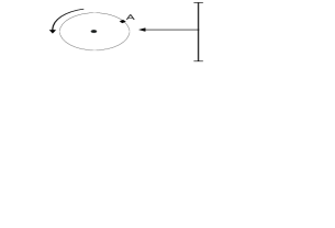
Figure 1: What is the probability that the rotating disk stops in such a way that the point $A$ will be exactly in front of the arrow?

However, the point $A$ can stop in front of the arrow, i.e., this event is not impossible and its probability should be strictly greater than zero, i.e., $P(E)>0$. Obviously, this example is a particular manifestation of the general fact that, if $\xi$ is any continuous random value and $a$ is any real number then $P(\xi=a)=0$. While for a discrete random variable one could say that an event with probability zero is impossible, this can not be said in the terms of the traditional probability theory for any continuous random variable.

Let us see what we can say with respect to this problem by using the new methodology. The problem under consideration deals with points located on the circumference $C$ of the disk. Thus, we need a definition of the term ‘point’ and mathematical tools allowing us to indicate a point on the circumference. If we accept (as is usually done in modern Mathematics) that a point is determined by a numeral $x$ called the coordinate of the point where $x\in\mathcal{S}$ and $\mathcal{S}$ is a set of numerals, then we can indicate the point by its coordinate $x$ and are able to execute required calculations. The choice of the numeral system $\mathcal{S}$ defines both the kind of numerals expressible in this system and the quantity (finite or infinite) of these numerals (see [22, 23] for a detailed discussion). As a consequence, we are not able to work with those points which coordinates are not expressible in the chosen numeral system $\mathcal{S}$ (recall Postulate 2).

Different numeral systems can be chosen to express coordinates of the points in dependence on the precision level we want to obtain. In some sense, the situation with counting points is similar to the work with a microscope: we decide the level of the precision we need and obtain a result dependent on the chosen level. If we need a more precise or a more rough answer, we change the level of the accuracy of our microscope. In the moment when we have have decided which lens (numeral system) we put in the microscope we decide which objects (points, arcs, etc.) we are able to observe, to measure, and to work with.

The formalization of the concept ‘point’ introduced above allows us to execute more accurate computations having, as it always happens in any process of the measurement, their own accuracy. Suppose that we have chosen a numeral system $\mathcal{S}$ allowing one to observe $K$ points on the circumference. Definition of the notion point allows us to define elementary events in our experiment as follows: the disk has stopped and the arrow indicates a point. As a consequence, we obtain that the number, $N(\Omega)$, of all possible elementary events, $e_{i}$, in our experiment is equal to $K$ where $\Omega=\cup_{i=1}^{N(\Omega)}e_{i}$ is the sample space of our experiment. If our disk is well balanced, all elementary events are equiprobable and, therefore, they have the same probability equal to $\frac{1}{N(\Omega)}$ and the accuracy of any further computation with this probabilistic model will be equal to $\frac{1}{N(\Omega)}$. Thus, we can calculate $P(E)$ directly by subdividing the number, $N(E)$, of favorable elementary events by the number, $K=N(\Omega)$, of all possible events.

For example, if we use numerals of the type $\frac{i\cdot 2\pi r}{\hbox{$\displaystyle{\mbox{\char 172}}$}},i\in\mathbb{N},$ then $K=\hbox{$\displaystyle{\mbox{\char 172}}$}$ and, since the number of the points is infinite and the length of the circumference is finite, our points are infinitesimally close, i.e., the probabilistic model is continuous. The chosen numerals define the accuracy of the model and do not allow us to answer to questions regarding objects having an extension on the circumference that is less than $\frac{2\pi r}{\hbox{$\displaystyle{\mbox{\char 172}}$}}$.

The number $N(E)$ depends on our decision about how many numerals we want to use to represent the point $A$. If we decide that the point $A$ on the circumference is represented by $m$ numerals we obtain

$$P(E)=\frac{N(E)}{N(\Omega)}=\frac{m}{K}=\frac{m}{\hbox{$\displaystyle{\mbox{\char 172}}$}}>0.$$

where the number $\frac{m}{\hbox{$\displaystyle{\mbox{\char 172}}$}}$ is infinitesimal if $m$ is finite. Note that this representation is very interesting also from the point of view of distinguishing the notions ‘point’ and ‘arc’. When $m$ is finite than we deal with a point, when $m$ is infinite we deal with an arc.

In the case we need the probabilistic model with a higher accuracy, we can choose, for instance, numerals of the type $\frac{i\cdot 2\pi r}{\hbox{$\displaystyle{\mbox{\char 172}}$}^{-2}},1\leq i\leq\hbox{$\displaystyle{\mbox{\char 172}}$}^{2},$ for expressing points on the circumference. In this way we also obtain a continuous model with the order that is higher than in the previous case. It follows $K=\hbox{$\displaystyle{\mbox{\char 172}}$}^{2}$ and for a finite $m$ we obtain the infinitesimal probability $P(E)=\frac{m}{\hbox{$\displaystyle{\mbox{\char 172}}$}^{2}}>0$.

In contrast, if we need a rough probabilistic model and decide to work with a finite number, $K$, of points on the circumference, then we have the discrete model. In this case, the probability $P(E)$ will be finite, and the model does not allow us to answer to questions regarding objects having an extension on the circumference that is less than $\frac{2\pi r}{K}$.

As we have shown by the example above, in our approach, for both cases, the discrete and the continuous one, only the impossible event has the probability equal to zero. All other events have positive probabilities that can be finite or infinitesimal in dependence of the accuracy of the chosen probabilistic model. Thus, the obtained probabilities are not absolute, i.e., there is again a straight analogy with Physics where results of the observation have a precision determined by the used instrument. Moreover, the new approach allows us to look at the same mathematical object (like it happens in Physics for physical objects) as continuous or discrete in dependence on the chosen instrument of the observation (see [22] for a detailed discussion related to this issue).

References

- [1] Cantor G., Contributions to the Founding of the Theory of Transfinite Numbers, Dover Publications, New York 1955.
- [2] Carroll J.B. (Ed.), Language, Thought, and Reality: Selected Writings of Benjamin Lee Whorf, MIT Press, 1956.
- [3] Cauchy A.L., Le Calcul infinitésimal, Paris 1823.
- [4] Conway J.H. and Guy R.K., The Book of Numbers, Springer-Verlag, New York 1996.
- [5] d’Alembert J., Différentiel, Encyclopédie, ou dictionnaire raisonné des sciences, des arts et des métiers, 4, Paris (1754).
- [6] Gödel K., The Consistency of the Continuum-Hypothesis, Princeton University Press, Princeton 1940.
- [7] Gödel K., Über formal unentscheidbare Sätze der Principia Mathematica und verwandter Systeme, Monatshefte für Mathematik und Physik 38 (1931), 173–198.
- [8] Gordon P., Numerical Cognition without Words: Evidence from Amazonia, Science 306 (15 October) (2004), 496–499.
- [9] Hardy G.H., Orders of infinity, Cambridge University Press, Cambridge 1910.
- [10] Hilbert D., Mathematical Problems: Lecture delivered before the International Congress of Mathematicians at Paris in 1900, Bulletin of the American Mathematical Society 8 (1902), 437–479.
- [11] Knopp K., Theory and Application of Infinite Series, Dover Publications, New York 1990.
- [12] Leibniz G.W. and Child J.M., The Early Mathematical Manuscripts of Leibniz, Dover Publications, New York 2005.
- [13] Mayberry J.P., The Foundations of Mathematics in the Theory of Sets, Cambridge Univ. Press, Cambridge 2001.
- [14] Newton I., Method of Fluxions, 1671.
- [15] Pica P., Lemer C., Izard V., Dehaene S., Exact and Approximate Arithmetic in an Amazonian Indigene Group, Science 306 (15 October) (2004), 499–503.
- [16] Robinson A., Non-Standard Analysis, Princeton Univ. Press, Princeton 1996.
- [17] Sapir E., Selected Writings of Edward Sapir in Language, Culture and Personality, University of California Press, Princeton 1958.
- [18] Sergeyev Ya.D., Arithmetic of Infinity, Edizioni Orizzonti Meridionali, CS 2003.
- [19] Sergeyev Ya.D., Blinking Fractals and Their Quantitative Analysis Using Infinite and Infinitesimal Numbers, Chaos, Solitons Fractals. 33 1 (2007), 50–75.
- [20] Sergeyev Ya.D., A New Applied Approach for Executing Computations with Infinite and Infinitesimal Quantities, Informatica 19 4 (2008), 567–596.
- [21] Sergeyev Ya.D., Evaluating the Exact Infinitesimal Values of Area of Sierpinski’s Carpet and Volume of Menger’s Sponge, Chaos, Solitons Fractals 42 5 (2009), 3042–3046.
- [22] Sergeyev Ya.D., Numerical Point of View on Calculus for Functions Assuming Finite, Infinite, and Infinitesimal Values Over Finite, Infinite, and Infinitesimal Domains, Nonlinear Analysis Series A: Theory, Methods Applications 71 12 (2009), e1688–e1707
- [23] Sergeyev Ya.D., Numerical Computations and Mathematical Modelling with Infinite and Infinitesimal Numbers, J. Applied Mathematics Computing 29 (2009), 177–195.
- [24] Sergeyev Ya.D., Computer System for Storing Infinite, Infinitesimal, and Finite Quantities and Executing Arithmetical Operations with Them, EU patent 1728149 (2009).
- [25] Sergeyev Ya.D., Counting Systems and the First Hilbert Problem, Nonlinear Analysis Series A: Theory, Methods Applications 72 3-4 (2010), 1701–1708.
- [26] Sergeyev Ya.D. and Garro A., Observability of Turing Machines: A Refinement of the Theory of Computation Informatica (2010) (in press).
- [27] The Infinity Computer web page, http://www.theinfinitycomputer.com