Solutions of the Gross-Pitaevskii and time-fractional Gross-Pitaevskii equations for different potentials with Homotopy Perturbation Method

Abstract

In this study, after we have briefly introduced the standard Gross-Pitaevskii equation, we have suggested fractional Gross-Pitaevskii equations to investigate the time-dependent ground state dynamics of the Bose-Einstein condensation of weakly interacting bosonic particle system which can includes non-Markovian processes or non-Gaussian distributions and long-range interactions. Only we focused the time-fractional Gross-Pitaevskii equation and have obtained solutions of the standard Gross-Pitaevskii and time-fractional Gross-Pitaevskii equations for attractive and repulsive interactions in the case external trap potentials $V(x)=0$ and optical lattice potential $V\left(x\right)=\pm\sin^{2}x$ by using Homotopy Perturbation Method. We have found that the Homotopy Perturbation Method solutions of the Gross-Pitaevskii equation for these potentials and interactions are the same analytical results of it. Furthermore we have also found that solutions of the time-fractional Gross-Pitaevskii equation for these potentials and interactions can be given in terms of Mittag-Leffler function. The solutions of the time-fractional Gross-Pitaevskii equation provide that the time evolution of the ground state dynamics of Bose-Einstein condensation of bosonic particles deviates exponential form, and evolutes with time as stretched exponentially.

1 Introduction

The zero temperature Bose-Einstein condensation (BEC) of dilute or weakly interacting bosons are generally described by Gross-Pitaevskii equation which is s a self-consistent mean field nonlinear Schrödinger equation [1, 2]. It is clearly known that this equation does not include memory effects of the non-Markovian processes, non-Gaussian distribution of particles, the long-range inter-particle interaction effects or the fractal structure of the interacting space between particles in condensate phase. However, it is shown that some experimental observations in a real real dilute or weakly interacting bosonic systems deviates from theoretical predictions i.e. some experimental results do not comply with theoretical calculations. For example, for dilute atomic gases that involve interacting atoms or molecules such as ⁸⁷Rb, ²³Na and ⁷Li which are trapped in a harmonic oscillator potential, there are significant differences between the theoretical and experimental transition temperatures in Bose-Einstein condensation. Similarly, for ⁴He, the experimentally observed value of the transition temperature to BEC is $T_{c}=2.17$ K, whereas the calculated one is $T_{c}=3.10$ K in conventional Bose-Einstein thermostatistics [4, 5, 6, 7, 8, 9]. These contractions between experimental observation and theoretical predictions shows that the memory effects of the non-Markovian processes, non-Gaussian distribution of particles, the long-range inter-particle interaction effects or the fractal structure of the interacting space in real bosonic systems have a predominant role below the critical temperature $T_{c}$ [3]. For this reason, we can claim that this standard approaches remain insufficient in the investigation ground state dynamics of the physical behavior of weakly interacting quantum boson gases at low temperatures i.e. below the $T_{c}$. At finite temperature below the $T_{c}$ and even though at zero temperature, the non-Markovian processes, non-Gaussian distribution of particles, the long-range effects between particles or the fractal structure of the interacting space in the Bose-Einstein condensate phase must be taken into account in the model. However, to the best of our knowledge on the literature, there does not exist a sound mathematical basis for these efforts in the literature.

In this study, we will adopt fractional calculus, which involves fractional derivatives and integrals. With the help of fractional calculus, it is possible to take into account memory effects of the non-Markovian processes, non-Gaussian distribution of particles, the long-range inter-particle interaction effects or the fractal structure of the interacting space [3, 10, 11]. Because in the fractional calculus concept, these unusual effects that are disappearing in the Markovian process can be represented the space-fractional and time-fractional derivative operators [12, 13]. Therefore, here we will define fractional Gross-Pitaevskii equations, and we will focus only time-fractional Gross-Pitaevskii equation to investigate ground state dynamics of the Bose-Einstein condensate of dilute or weakly interacting boson gas has repulsive or attractive interactions for zero external potential and optical lattice potentials at zero temperature.

As it is known that time-dependent Gross-Pitaevskii equation is a nonlinear partial differential equation and it is difficult to find analytical solution of this type of equation for especially complex potentials. Therefore, the numerical solution methods are generally used to find solution of them. In order to solve fractional ordinary differential equation, integral equation and fractional partial differential equations in physics and other areas of science, several analytical and numerical methods have been proposed. The most commonly used ones are; Adomain Decomposition Method (ADM) [14, 15, 16, 17, 18, 19], Variational Iteration Method (VIM) [17, 18, 19, 20, 21], Fractional Difference Method (FDM) [22], Differential Transform Method (DTM) [23], Homotopy perturbation Method (HPM) [24, 25]. Also there are some classical solution techniques e.g. Laplace transform method, Fractional Green’s function method, Mellin transform method and method of orthogonal polynomials [22]. In this study, we will use the HPM method to solve fractional Gross-Pitaevskii equations. HPM has been proposed by He [26, 27] to solve linear and nonlinear differential and integral equations. This method, which is a coupling of the traditional perturbation method and homotopy in topology, deform continuously to simple problem which easily solved. The HPM can be easily applied to Volterra’s integro-differential equation [28], to nonlinear oscillators [29], bifurcation of nonlinear problems [30], bifurcation of delay-differential equations [31], nonlinear wave equations [32], boundary value problems [33], quadratic Ricatti differential equation of fractional order [24] and to other fields [34, 35, 36, 37, 38, 39, 40, 41, 42]. This HPM yield very convergence of the solution series in most cases, usually only a few iteration leading to very accurate solutions.

This paper is organized as follows. In Section 2 we briefly review Gross-Pitaevskii equation. In Section 3, we present the stationary solution of the Gross-Pitaevskii equation. In Section 4, we define Gross-Pitaevskii equation with fractional orders. In Section 5, we summarize basic definition of the fractional calculus. In Section 6, the Homotopy perturbation method is introduced. In Section 7, we discuss several example. Finally Section 8 is devoted to conclusions.

2 Gross-Pitaevskii equation

The properties of a Bose-Einstein condensate at zero temperature are well described by the macroscopic wave-function $\psi\left(x,t\right)$ whose evolution is governed by the Gross-Pitaevskii equation [1, 2] which is a self-consistent mean field nonlinear Schrödinger equation:

$$i\hbar\frac{\partial}{\partial t}\psi\left(x,t\right)=\left(-\frac{\hbar^{2}}{2m}\nabla^{2}+V\left(x\right)+g\left|\psi\left(x,t\right)^{2}\right|\right)\psi\left(x,t\right)\ ,\quad x\in\Omega\subseteq R^{d}$$ (1)

$$\psi\left(x,t\right)=0\ ,\quad x\in\Gamma=\partial\Omega,$$ (2)

$$\psi\left(x,0\right)=\psi_{0}\left(x\right)\ ,\quad x\in\Omega;$$ (3)

where $g$, $m$ and $V\left(x\right)$ are the interacting parameter between particles, mass of the particles and external potential applying to the particle systems, respectively. The interacting parameter i.e. coupling constant $g$ is defined as $g=4\pi\hbar a_{s}/m$ where $a_{s}$ the scattering length of two interacting bosons. Coupling constant determines the interaction types between particles. For $g<0$ and $g>0$ interactions between bosonic particles are attractive and repulsive, respectively.

It is known that there are two important invariant of Eq. (1) which are the normalization of the wave-function

$$N\left(\psi\right)=\int_{\Omega}\left|\psi\left(x,t\right)\right|^{2}dx\equiv N\left(\psi_{0}\right)=\int_{\Omega}\left|\psi_{0}\left(x\right)\right|^{2}dx=1\ ,\quad t\geq 0$$ (4)

and the energy functional for $t\geq 0$

$$E\left(\psi\right)=\int_{\Omega}\left[\frac{1}{2}\left|\nabla\psi\left(x,t\right)\right|^{2}+V\left(x\right)\left|\psi\left(x,t\right)\right|^{2}+\frac{g}{2}\left|\psi\left(x,t\right)\right|^{4}\right]dx\equiv E\left(\psi_{0}\right)$$ (5)

where $N\left(\psi\right)$ is particle number and $E\left(\psi\right)$ is the energy of the particle systems in condensate phase. It can be seen from Eq. (5) the energy functional $E\left(\psi\right)$ consist of the three parts i.e., kinetic energy, potential energy and interacting energy.

The magnitude square of the eigenfunction, $\left|\psi\left(x,t\right)\right|^{2}$, represents the probability density of finding a particle at position $x$ and time $t$. Stationary state of the Bose-Einstein condensed system is the independent of the time. To find stationary solution of Eq. (1), we write the wave function as

$$\psi\left(x,t\right)=\psi\left(x\right)e^{-i\mu t/\hbar}$$ (6)

where $\mu$ is the chemical potential of the condensate and $\psi\left(x\right)$ is a function independent of time. Substituting (6) into (1) yield the equation

$$\mu\psi\left(x\right)=\left(-\frac{1}{2}\nabla^{2}+V\left(x\right)+g\left|\psi\left(x\right)^{2}\right|\right)\psi\left(x\right)\ ,\quad x\in\Omega\subseteq R^{d}$$ (7)

for $\psi\left(x\right)$ under the normalization condition

$$\left\|\psi\right\|=\int_{\Omega}\left|\psi\left(x\right)\right|^{2}dx=1$$ (8)

On the other hand, any eigenvalue $\mu$ can be computed from its corresponding eigenfunction $\psi$ by

$$\mu=\mu\left(\psi\right)=\int_{\Omega}\left[\frac{1}{2}\left|\nabla\psi\left(x\right)\right|^{2}+V\left(x\right)\left|\psi\left(x\right)\right|^{2}+g\left|\psi\left(x\right)\right|^{4}\right]dx\ .$$ (9)

3 Soliton or stationary solutions of the Gross-Pitaevskii equation

The most simple solution of the Eq. (1) is the stationary solution of its for $V\left(x\right)=0$. When $d=1$, $V\left(x\right)=0$ the soliton solutions can be obtained (See [2]). For repulsive interactions i.e. $g>0$ the solution of Eq. (1) is given by

$$\psi_{d}\left(x\right)=\psi_{d}\left(x,0\right)=\sqrt{\frac{\mu}{g}}\tan h\left(\sqrt{\mu}x\right)$$ (10)

This solution is known as dark solution. Hence we can write the time-dependent dark soliton as

$$\psi_{d}\left(x,t\right)=\sqrt{\frac{\mu}{g}}\tan h\left(\sqrt{\mu}x\right)e^{-i\mu t/\hbar}$$ (11)

which corresponds to a local minimum of the density distribution $\left|\psi\left(x,t\right)\right|^{2}$. On the other hand, for attractive interactions i.e. $g<0$, the solution of the Eq. (1) is given by

$$\psi_{b}\left(x\right)=\psi_{b}\left(x,0\right)=\sqrt{\frac{\mu}{g}}\sec h\left(\sqrt{\mu}x\right)\ .$$ (12)

This solution is known as bright solution. Similarly, time-dependent bright soliton solution is given by

$$\psi_{b}\left(x,t\right)=\sqrt{\frac{\mu}{g}}\sec h\left(\sqrt{\mu}x\right)e^{-i\mu t/\hbar}\$$ (13)

which corresponding to a local maximum of the density distribution $\left|\psi\left(x,t\right)\right|^{2}$. These solutions can be generalized easily in the progressive wave form. Generalized dark soliton solution of Eq. (1) can be written in the one-dimensional form

$$\psi\left(x,t\right)_{d}=\sqrt{\frac{\mu}{g}}\tan h\left[\sqrt{\mu}\left(x-vt-x_{0}\right)\right]e^{-i\mu t/\hbar}$$ (14)

and similarly generalized bright solution solution of Eq. (1) is given by

$$\psi\left(x,t\right)_{b}=\sqrt{\frac{\mu}{g}}\sec h\left[\sqrt{\mu}\left(x-vt-x_{0}\right)\right]e^{-i\mu t/\hbar}$$ (15)

where $v$ is the speed of the soliton. Also $x_{0}$ and $t_{0}$ are respectively initial position and time. Solitons are quantized vertex in Bose-Einstein condensate system, which can be observation experimentally. The shape of the solitons are change depending on external potential. We here discussed only $V\left(x\right)=0$ case for simplicity.

4 Gross-Pitaevskii equations with fractional derivatives

We remark in introduction that the memory effects of the non-Markovian processes, non-Gaussian distribution of particles, the long-range inter-particle interaction effects or the fractal structure of the interacting in a bosonic system below the condensate temperature $T_{c}$ space can leads to fractional dynamics. Simply we say that all non-Markovian stochastic processes of the particles or waves in condensate phase of bosonic system generate the time-fractional Gross-Pitaevskii equation ignoring boundary conditions and sources. Similarly, non-Gaussian distribution of the particles or waves in condensate phase leads to space-fractional Gross-Pitaevskii equation. On the other hand the combination of the non-Markovian and non-Gaussian behavior yield time and space-fractional Gross-Pitaevskii equation. These equation are defined in Ref. [3]. In the light of these knowledge, the one-dimensional time-fractional Gross-Pitaevskii equation can be written in the form

$$i\hbar\psi\left(x,t\right)=\ _{0}D_{t}^{1-\alpha}\left(-\frac{\hbar^{2}}{2m}\nabla^{2}+V\left(x\right)+g\left|\psi\left(x,t\right)^{2}\right|\right)\psi\left(x,t\right)$$ (16)

where ${}_{0}D_{t}^{1-\alpha}$ is the Riemann-Liouville fractional integral operator. Similarly the one-dimensional space-fractional Gross-Pitaevskii equation can be defined as

$$i\hbar\frac{\partial}{\partial t}\psi\left(x,t\right)=\left(-\frac{\hbar^{2}}{2m}\nabla^{\beta}+V\left(x\right)+g\left|\psi\left(x,t\right)^{2}\right|\right)\psi\left(x,t\right)\ .$$ (17)

Finally we can write time and space-fractional Gross-Pitaevskii equation in the one-dimensional form

$$i\hbar\psi\left(x,t\right)=\ _{0}D_{t}^{1-\alpha}\left(-\frac{\hbar^{2}}{2m}\nabla^{\beta}+V\left(x\right)+g\left|\psi\left(x,t\right)^{2}\right|\right)\psi\left(x,t\right)\ .$$ (18)

Here we focus solutions of the time-fractional Gross-Pitaevskii equation for different potentials. But we will consider other cases of these equations for different potential in the another study.

5 Basic definitions for fractional calculus

Before we discuss solution of the time-fractional Gross-Pitaevskii equation (16) we will give basic rules for calculating fractional differential equations in this section. Some definitions for fractional calculus are given below [22, 43, 44, 45, 46, 47, 48].

Definition 1

The Riemann-Liouville fractional integral operator of order $\alpha\geq 0$ of the function $f(t)\in C_{\mu}$ is defined as for $\mu\geq-1$

$${}_{t_{0}}D_{t}^{-\alpha}f\left(t\right)=\frac{1}{\Gamma\left(\alpha\right)}\int_{t_{0}}^{t}dt^{\prime}\frac{f\left(t^{\prime}\right)}{\left(t-t^{\prime}\right)^{1-\alpha}},\ \quad\alpha>0,\ \quad t>0$$ (19)

where ${}_{t_{0}}D_{t}^{-\alpha}f\left(t\right)$ is the Riemann-Liouville fractional integral operator which is a direct extension of Cauchy’s multiple integral for arbitrary complex $\alpha$ with $Re\left(\alpha\right)>0$. A fractional derivative is then established via a fractional integration and successive ordinary differential according to

$${}_{t_{0}}D_{t}^{\beta}f\left(t\right)=\frac{d^{n}}{dt^{n}}D_{t}^{\beta-n}f\left(t\right)$$ (20)

with $Re\left(\beta\right)>0$, and the natural number $n$ satisfies the inequality $n\geq Re\left(\beta\right)>n-1$. Two special cases are the Riemann-Liouville ${}_{0}D_{t}^{\beta}$ for $t_{0}=0$ and Weyl operator ${}_{-\infty}D_{t}^{\mu}$ for $t_{0}=-\infty$. The Riemann-Liouville operator for $t_{0}=0$ is given by

$${}_{0}D_{t}^{\alpha}f\left(t\right)=\frac{1}{\Gamma\left(n-\alpha\right)}\frac{d^{n}}{dt^{n}}\int_{0}^{t}dt^{\prime}\frac{f\left(t^{\prime}\right)}{\left(t-t^{\prime}\right)^{1-n-\alpha}},\quad n\geq Re(\alpha)>n-1.$$ (21)

For any function $f\left(x,t\right)$ the fractional Riemann-Liouville differintegration ${}_{0}D_{t}^{1-\alpha}=\left(\partial/\partial t\right)_{0}D_{t}^{-\alpha}$ is defined through the relation

$${}_{0}D_{t}^{1-\alpha}f\left(x,t\right)=\frac{1}{\Gamma\left(\alpha\right)}\frac{\partial}{\partial t}\int_{0}^{t}dt^{\prime}\frac{f\left(x,t^{\prime}\right)}{\left(t-t^{\prime}\right)^{1-\alpha}}\ .$$ (22)

This differintegration operator of an arbitrary power for $t_{0}=0$ is given by

$${}_{0}D_{t}^{\nu}t^{\mu}=\frac{\Gamma\left(1+\mu\right)}{\Gamma\left(1+\mu-\nu\right)}t^{\mu-\nu}$$ (23)

which coincides with the heuristic generalization of the standard differentiation

$$\frac{d^{n}t^{m}}{dt^{n}}=\frac{m!}{\left(m-n\right)!}t^{m-n}$$ (24)

by introduction of Gamma function. An interesting consequence of Eq. (22) is the nonvanishing fractional differintegration of a constant $a$

$${}_{0}D_{t}^{\nu}a=\frac{1}{\Gamma\left(a-\nu\right)}t^{-\nu}\ .$$ (25)

The Riemann-Liouville differentiation of exponential function leads to

$${}_{0}D_{t}^{\nu}e^{t}=\frac{t^{-\nu}}{\Gamma\left(1-\nu\right)}F_{1,1}\left(1,1-\nu,t\right)$$ (26)

involving the confluent hypergeometric function $F_{1,1}$.

Definition 2

The Caputo fractional derivative operator [49] is given by

$${}_{t_{0}}^{C}D_{t}^{\alpha}f\left(t\right)=\frac{1}{\Gamma\left(\alpha-n\right)}\int_{t_{0}}^{t}dt^{\prime}\frac{f^{\left(n\right)}\left(t^{\prime}\right)}{\left(t-t^{\prime}\right)^{\alpha+1-n}},\quad n-1<\alpha<n$$ (27)

Under natural condition on the function $f\left(t\right)$, for $\alpha\rightarrow n$ the Caputo derivative becomes a conventional $n$-th derivative of the function $f\left(t\right)$.

The Riemann-Liouville fractional operator (22) and Caputo’s fractional operators (27) have different form. Another difference between these operators is that the Caputo derivative of a constant is $0$, whereas the Riemann-Liouville fractional derivative of a constant is given by Eq. (25). On the other hand, the main advantage of Caputo’s approach is that the initial conditions for fractional differential equations with Caputo derivatives take some form as for integer-order differential equations.

Definition 3

The Mittag-Leffler function [50, 51] $E_{\alpha}\left(z\right)$ is a complex function which depends on on two complex parameters $\alpha$ and $\beta$. It may be defined by the following series representation when $\alpha>0$, valid in the whole complex plane

$$E_{\alpha,\beta}\left(z\right)=\sum_{n=0}^{\infty}\frac{z^{n}}{\Gamma\left(\alpha n+\beta\right)},\quad\alpha>0,\quad z\in C$$ (28)

In the case $\alpha$ and $\beta$ are real and positive, the series converges for all values of the argument $z$, so the Mittag-Leffler function is an entire function. Some special cases of the Mittag-Leffler function are follow. The Mittag-Leffler function is the natural generalization of the exponential function. Being a special case of the Fox function introduced below, it is defined through the inverse Laplace transform

$$E_{\alpha}\left(-\left(t/\tau\right)^{\alpha}\right)=\pounds^{-1}\left\{\frac{1}{u+\tau^{-\alpha}u^{1-\alpha}}\right\}$$ (29)

from which the series expansion

$$E_{\alpha}\left(-\left(t/\tau\right)^{\alpha}\right)=\sum_{n=0}^{\infty}\frac{\left(-\left(t/\tau\right)^{\alpha}\right)^{n}}{\Gamma\left(1+\alpha n\right)}$$ (30)

can be deduced, where $\tau$ is a constant. The asymptotic behavior of the Mittag-Leffler function interpolates between the initial stretched exponential form

$$E_{\alpha}\left(-\left(t/\tau\right)^{\alpha}\right)\sim\exp\left(-\frac{\left(t/\tau\right)^{\alpha}}{\Gamma\left(1+\alpha\right)}\right)$$ (31)

for $t<\tau$ and the long-time inverse power-law behavior as

$$E_{\alpha}\left(-\left(t/\tau\right)^{\alpha}\right)\sim\left(\frac{t}{\tau}\right)^{\alpha}\frac{1}{\Gamma\left(1-\alpha\right)}$$ (32)

for $t\gg\tau$, $0<\alpha<1$. Special cases of the Mittag-Leffler function are the exponential function

$$E_{1}\left(-t/\tau\right)=e^{-t/\tau}$$ (33)

and the product of the exponential and the complementary error function

$$E_{1/2}\left(-\left(t/\tau\right)^{1/2}\right)=e^{-t/\tau}erfc\left(\left(t/\tau\right)^{1/2}\right)\ .$$ (34)

6 Solution of Gross-Pitaevskii equations of integer and fractional order with HPM

The principles of HPM and its applicability for various kinds of differential equations ar given in [24, 25, 26, 27, 28, 29, 30, 33, 34, 35, 36, 37, 38, 39, 40, 41, 42]. Here after we present a review of the standard HPM and modified HPM suggested by Momani and Odibat [24, 25]. We will employe HPM to the Gross-Pitaevskii equations of integer order and fractional order.

6.1 HPM for Gross-Pitaevskii equation of integer order

To explain the basic ideas of this method on nonlinear differential equation of integer order, we consider one-dimensional Gross-Pitaevskii equation in the form Eq. (1) and adopt the homotopy perturbation method to this equation. Gross-Pitaevskii equation (1) is a nonlinear partial differential equation which can be decomposed as linear and nonlinear part:

$$L\left(\psi\left(x,t\right)\right)+N\left(\psi\left(x,t\right)\right)=f\left(x,t\right),\quad x\in\Omega,\quad t>0$$ (35)

where $L(\psi)$ is a linear part and $N(\psi)$ is a nonlinear part and on the other hand $f\left(x,t\right)$ is known analytical function of Eq. (1). For $f\left(x,t\right)=0$, $L(\psi)$ and $N(\psi)$ can be defined follow as

$$L\left(\psi\right)=i\hbar\frac{\partial\psi\left(x,t\right)}{\partial t},\quad N\left(\psi\right)=+\frac{\hbar^{2}}{2m}\nabla^{2}\psi\left(x,t\right)+V\left(x\right)\psi\left(x,t\right)+g\left|\psi\left(x,t\right)^{2}\right|\psi\left(x,t\right).$$ (36)

We note that Eq. (35) must be defined with the boundary condition

$$B(\psi(x),\ \partial\psi(x)/\partial n)=0,\ x\in\Gamma$$ (37)

where $\Gamma$ is the boundary of the domain $\Omega$. Homotopy perturbation method defines the homotopy $\phi\left(x,p\right):\Omega\times\left[0,1\right]\rightarrow R$ which satisfies

$$H\left(\phi,p\right)=\left(1-p\right)\left[L\left(\phi\right)-L\left(\psi_{0}\right)\right]+p\left[L\left(\phi\right)+N\left(\phi\right)-f\left(x,t\right)\right]=0$$ (38)

or

$$H\left(\phi,p\right)=L\left(\phi\right)-L\left(\psi_{0}\right)+pL\left(\psi_{0}\right)+p\left[N\left(\phi\right)-f\left(x,t\right)\right]=0$$ (39)

where $p\in[0,1]$ is an embedding parameter, $\psi_{0}=\psi(x,0)$ is an initial guess of exact solution $\psi(x,t)$, which is independent of time and satisfies the boundary conditions. Hence from Eqs. (38) and (39) we obtain

$$H(\phi,0)=L(\phi)-L(\psi_{0}(x))=0$$ (40)

$$H(\phi,1)=L(\psi_{0})+N(\phi)-f(x,t)=0\ .$$ (41)

Changing process $p$ from zero to unity is just that of $\phi(x,p)$ from $\psi_{0}(x)$ to $\phi(x,t)$. In topology, this is known as homotopy [24, 25, 26, 27], $L(\phi)-L(\psi_{0}(x))$ and $L(\psi_{0})+N(\phi)-f(x,t)$ are homotopic. This basic assumption is that the solution of Eqs. (38) or (39) can be expressed as a power series in $p$:

$$\phi\left(x,p\right)=\phi_{0}\left(x\right)+p\phi_{1}\left(x\right)+p^{2}\phi_{2}\left(x\right)+...$$ (42)

The approximation solution of Eqs. (1) or (35) can be obtained in the limit $p\rightarrow 1$ as

$$\psi\left(x,t\right)=\phi\left(x,p\right)_{p\rightarrow 1}=\phi_{0}\left(x\right)+p\phi_{1}\left(x\right)+p^{2}\phi_{2}\left(x\right)+...\ .$$ (43)

As a consequence, the final result of standard Gross-Pitaevskii equation in the form Eq. (1) is given

$$\psi\left(x,t\right)=\sum_{j=0}^{\infty}p^{j}\phi_{j}\left(x\right)$$ (44)

when $p\rightarrow 1$. Here we note that the solution function $\phi_{k}\left(x\right)$ includes the constants of the Eq. (1). On the other hand, we say that the convergence of the series (44) has been proved for many nonlinear ordinary and partial differential equations [26, 34].

After a brief introduce of HPM, now we can apply HPM to the Gross-Pitaevskii equation of integer order. To solve Eq. (1), using Eq. (38) we construct the following homotopy:

$$\left(1-p\right)\left(\frac{\partial\phi}{\partial t}-\frac{\partial\psi_{0}}{\partial t}\right)+p\left[\frac{\partial\phi}{\partial t}-\frac{i}{\hbar}\left(\frac{\hbar}{2m}\nabla^{2}\phi-V\left(x\right)\phi-g\left|\phi^{2}\right|\phi\right)\right]=0.$$ (45)

Substituting Eq. (42) into Eq. (45) and equating the coefficients of the terms with the identical powers of $p$,

$$p^{0}:\ \frac{\partial\phi_{0}}{\partial t}-\frac{\partial\psi_{0}}{\partial t}=0,\quad\phi_{0}\left(x,0\right)=\psi_{0}\left(x\right)=\psi\left(x,0\right)$$ (46)

$$p^{1}:\ \frac{\partial\phi_{1}}{\partial t}-\frac{i}{\hbar}\left(\frac{\hbar}{2m}\nabla^{2}\phi_{0}-V\left(x\right)\phi_{0}-g\left|\phi_{0}^{2}\right|\phi_{0}\right)=0$$ (47)

$$p^{2}:\ \frac{\partial\phi_{2}}{\partial t}-\frac{i}{\hbar}\left(\frac{\hbar}{2m}\nabla^{2}\phi_{1}-V\left(x\right)\phi_{1}-g\sum_{i=0}^{1}\sum_{k=0}^{1-i}\left|\phi_{i}\right|\left|\phi_{k}\right|\phi_{1-k-i}\right)=0$$ (48)

$$p^{3}:\ \frac{\partial\phi_{3}}{\partial t}-\frac{i}{\hbar}\left(\frac{\hbar}{2m}\nabla^{2}\phi_{2}-V\left(x\right)\phi_{2}-g\sum_{i=0}^{2}\sum_{k=0}^{2-i}\left|\phi_{i}\right|\left|\phi_{k}\right|\phi_{1-k-i}\right)=0$$ (49)

$$\begin{array}[]{c}.\\ .\\ .\end{array}$$

$$p^{j}:\ \frac{\partial\phi_{j}}{\partial t}-\frac{i}{\hbar}\left(\frac{\hbar}{2m}\nabla^{2}\phi_{j-1}-V\left(x\right)\phi_{j-1}-g\sum_{i=0}^{j-1}\sum_{k=0}^{j-i-1}\left|\phi_{i}\right|\left|\phi_{k}\right|\phi_{j-k-i-1}\right)=0$$ (50)

$$\begin{array}[]{c}.\\ .\\ .\end{array}$$

we get the iterative equation

$$\phi_{j}=\frac{i}{\hbar}\int_{0}^{t}\left(\frac{\hbar}{2m}\nabla^{2}\phi_{j-1}-V\left(x\right)\phi_{j-1}-g\sum_{i=0}^{j-1}\sum_{k=0}^{j-i-1}\left|\phi_{i}\right|\left|\phi_{k}\right|\phi_{j-k-1}\right)dt,\quad j=1,2,3,...$$ (51)

with initial value

$$\phi_{j}\left(x,0\right)=\psi\left(x\right)=\psi\left(x,0\right).$$ (52)

Hence all $\phi_{j}$ values can be obtained using Eq. (53). The final solution of Gross-Pitaevskii equation (1) of integer order can be written in terms of the Eq. (53) in the limit $p\rightarrow 1$:

$$\psi\left(x,t\right)=\frac{i}{\hbar}\sum_{j=0}^{\infty}p^{j}\int_{0}^{t}\left(\frac{\hbar}{2m}\nabla^{2}\phi_{j-1}-V\left(x\right)\phi_{j-1}-g\sum_{i=0}^{j-1}\sum_{k=0}^{j-i-1}\left|\phi_{i}\right|\left|\phi_{k}\right|\phi_{j-k-1}\right)dt\ .$$ (53)

HPM supposes that this solution satisfy Eq. (1) in the limit of the $p\rightarrow 1$.

6.2 HPM for time-fractional Gross-Pitaevskii equation

To solve the time-fractional Gross-Pitaevskii equation (16), we will apply HPM to Eq. (16). Hence we can construct the following homotopy

$$\left(1-p\right)\left({}_{0}D_{t}^{\alpha}\phi-\ _{0}D_{t}^{\alpha}\psi_{0}\right)+p\left[{}_{0}D_{t}^{\alpha}\phi-\frac{i}{\hbar}\left(\frac{\hbar}{2m}\nabla^{2}\phi-V\left(x\right)\phi-g\left|\phi^{2}\right|\phi\right)\right]=0$$ (54)

Suppose the solution of Eq. (56) to be as following form

$$\phi^{\alpha}\left(x,p\right)=\phi_{0}^{\alpha}\left(x\right)+p\phi_{1}^{\alpha}\left(x\right)+p^{2}\phi_{2}^{\alpha}\left(x\right)+...\ .$$ (55)

In the limit $p\rightarrow 1$ we can write solution of the time-fractional equation (16)

$$\psi^{\alpha}\left(x,t\right)=\sum_{j=0}^{\infty}p^{j}\phi_{j}^{\alpha}\left(x\right)\ .$$ (56)

Substituting Eq. (57) into Eq. (56) and equating the coefficients of the terms with identical powers of $p$, we obtain following equations

$$p^{0}:\ _{0}D_{t}^{\alpha}\phi_{0}^{\alpha}-\frac{\partial\psi_{0}^{\alpha}}{\partial t}=0$$ (57)

$$p^{1}:\ _{0}D_{t}^{\alpha}\phi_{1}^{\alpha}-\frac{i}{\hbar}\left(\frac{\hbar}{2m}\nabla^{2}\phi_{0}^{\alpha}-V\left(x\right)\phi_{0}^{\alpha}-g\left|\phi_{0}^{2}\right|\phi_{0}\right)=0$$ (58)

$$p^{2}:\ _{0}D_{t}^{\alpha}\phi_{2}^{\alpha}-\frac{i}{\hbar}\left(\frac{\hbar}{2m}\nabla^{2}\phi_{1}-V\left(x\right)\phi_{1}-g\sum_{i=0}^{1}\sum_{k=0}^{1-i}\left|\phi_{i}\right|\left|\phi_{k}\right|\phi_{1-k-i}\right)=0$$ (59)

$$p^{3}:\ _{0}D_{t}^{\alpha}\phi_{3}^{\alpha}-\frac{i}{\hbar}\left(\frac{\hbar}{2m}\nabla^{2}\phi_{2}-V\left(x\right)\phi_{2}-g\sum_{i=0}^{2}\sum_{k=0}^{2-i}\left|\phi_{i}\right|\left|\phi_{k}\right|\phi_{1-k-i}\right)=0$$ (60)

$$\begin{array}[]{c}.\\ .\\ .\end{array}$$ (61)

$$p^{j}:\ _{0}D_{t}^{\alpha}\phi_{j}^{\alpha}-i\left(\frac{\hbar}{2m}\nabla^{2}\phi_{j-1}-V\left(x\right)\phi_{j-1}-g\sum_{i=0}^{j-1}\sum_{k=0}^{j-i-1}\left|\phi_{i}\right|\left|\phi_{k}\right|\phi_{j-k-1}\right)=0$$ (62)

$$\begin{array}[]{c}.\\ .\\ .\end{array}$$ (63)

Finally we can write iterative relation as

$$\phi_{j}^{\alpha}=\frac{i}{\hbar\Gamma\left(\alpha\right)}\int_{0}^{t}\left(t-\tau\right)^{\alpha-1}\left(\frac{\hbar}{2m}\nabla^{2}\phi_{j-1}-V\left(x\right)\phi_{j-1}-g\sum_{i=0}^{j-1}\sum_{k=0}^{j-i-1}\left|\phi_{i}\right|\left|\phi_{k}\right|\phi_{j-k-1}\right)d\tau$$ (64)

with initial value

$$\phi_{j}^{\alpha}\left(x,0\right)=\psi\left(x\right)=\psi\left(x,0\right),\quad j=1,2,3,...\ .$$ (65)

The final solution of time-fractional Gross-Pitaevskii equation (16) can be given in terms of the Eq. (66) in the limit $p\rightarrow 1$:

$$\psi^{\alpha}\left(x,t\right)=\frac{i}{\hbar\Gamma\left(\alpha\right)}\sum_{j=0}^{\infty}p^{j}\int_{0}^{t}\left(t-\tau\right)^{\alpha-1}\left(\frac{\hbar}{2m}\nabla^{2}\phi_{j-1}^{\alpha}-V\left(x\right)\phi_{j-1}^{\alpha}-g\sum_{i=0}^{j-1}\sum_{k=0}^{j-i-1}\left|\phi_{i}^{\alpha}\right|\left|\phi_{k}^{\alpha}\right|\phi_{j-k-1}^{\alpha}\right)d\tau$$ (66)

HPM supposes that this solution satisfy the Eq. (16) in the limit of the $p\rightarrow 1$.

7 Numerical implementations for different potentials

Now we will investigate GP end time-fractional GP equations to discuss the ground state time-dependent dynamic of the Bose-Einstein condensation of weakly interacting system which involve attracting and repulsive interactions for different potential. In analysis we will use HPM to solve GP equations.

Example 1

Firstly we consider GP equation of integer and fractional order for $V\left(x\right)=0$ and repulsive interaction $g=1>0$. Hence we will discuss GPE of integer order in 1.Case-I and GPE of fractional order in 1.Case-II.

1.Case-I

For $V\left(x\right)=0$ and repulsive interaction $g=1>0$, the iterative equation (53) is given as

$$\phi_{j}=\frac{i}{\hbar}\int_{0}^{t}\left(\frac{\hbar}{2m}\nabla^{2}\phi_{j-1}-g\sum_{i=0}^{j-1}\sum_{k=0}^{j-i-1}\left|\phi_{i}\right|\left|\phi_{k}\right|\phi_{j-k-1}\right)dt\ .$$ (67)

For $g=1>0$, the HPM solutions of $\phi_{j}$ are given by

$$\phi_{0}=\tanh x$$ (68)

$$\phi_{1}=-\frac{-it}{\Gamma\left(2\right)}\tanh x$$ (69)

$$\phi_{2}=-\frac{t^{2}}{\Gamma\left(3\right)}\tanh x$$ (70)

$$\phi_{3}=-\frac{it^{3}}{\Gamma\left(4\right)}\tanh x$$ (71)

$$\begin{array}[]{c}.\\ .\\ .\end{array}$$ (72)

$$\phi_{n}=\left(-1\right)^{n}\frac{\left(it\right)^{n}}{\Gamma\left(n+1\right)}\tanh x$$ (73)

where we set $\hbar=m=1$ for simplicity. If we put these terms in the series expansion

$$\psi\left(x,t\right)=\phi_{0}\left(x\right)+p\phi_{1}\left(x\right)+p^{2}\phi_{2}\left(x\right)+...=\sum_{j=0}^{\infty}p^{j}\phi_{j}\left(x\right)$$ (74)

we obtain

$$\psi_{g>0}\left(x,t\right)=\tanh x+\sum_{n=1}^{\infty}\left(-1\right)^{n}\frac{\left(it\right)^{n}}{\Gamma\left(n+1\right)}\tanh x\ .$$ (75)

This solution can be represented in terms of Mittag-Leffler function for $\alpha=1$ as

$$\psi_{g>0}\left(x,t\right)=E_{1}\left[-\left(\frac{t}{\tau}\right)\right]\tanh x=\tanh xe^{-t/\tau}$$ (76)

where $i=1/\tau$. This unnormalized solution is of the same analytical form with Eq. (11) which corresponds dark soliton solution of GP equation. The numerical demonstration of the Eq. (78) fot $t=0$ and the probability density of $\psi_{g>0}\left(x,t\right)$ are given is given in Figs. (1a) and (1b), respectively. As it can be seen from Fig. (1b) when external potential $V\left(x\right)=0$, the probability density for attracting interactions has dark soliton form. These results confirm that obtained solution using HPM is the same with analytical solution of GP equation of integer order for $V\left(x\right)=0$ and $g>0$.

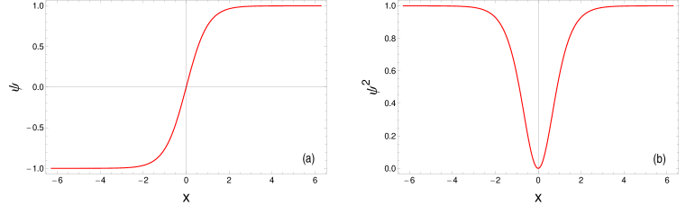
Figure 1: In the case $V\left(x\right)=0$ and $g>0$ a) Numerical representation of the $\psi_{g>0}\left(x,0\right)$, b) Numerical representation of the probability density of $\psi_{g>0}\left(x,t\right)$.

1.Case-II

Now we consider time-fractional GP equation for $V\left(x\right)=0$ and repulsive interaction i.e. $g>0$. The iterative equation (66) of the time-fractional GP equation for $V\left(x\right)=0$ and $g=1>0$ is given by

$$\phi_{j}^{\alpha}=\frac{i}{\hbar\Gamma\left(\alpha\right)}\int_{0}^{t}\left(t-\tau\right)^{\alpha-1}\left(\frac{\hbar}{2m}\nabla^{2}\phi_{j-1}^{\alpha}-g\sum_{i=0}^{j-1}\sum_{k=0}^{j-i-1}\left|\phi_{i}^{\alpha}\right|\left|\phi_{k}^{\alpha}\right|\phi_{j-k-1}^{\alpha}\right)d\tau\ .$$ (77)

In this case, the HPM solutions of $\phi_{j}^{\alpha}$ are given by

$$\phi_{0}^{\alpha}=\tanh x$$ (78)

$$\phi_{1}^{\alpha}=-\frac{it^{\alpha}}{\Gamma\left(\alpha+1\right)}\tanh x$$ (79)

$$\phi_{2}^{\alpha}=-\frac{t^{2\alpha}}{\Gamma\left(2\alpha+1\right)}\tanh x$$ (80)

$$\phi_{3}^{\alpha}=\frac{it^{3\alpha}}{\Gamma\left(3\alpha+1\right)}\tanh x$$ (81)

$$\begin{array}[]{c}.\\ .\\ .\end{array}$$ (82)

$$\phi_{n}^{\alpha}=\left(-1\right)^{n}\frac{\left(it^{\alpha}\right)^{n}}{\Gamma\left(n\alpha+1\right)}\tanh x$$ (83)

where we set $\hbar=m=1$ for simplicity. If we put these terms in the series expansion

$$\psi^{\alpha}\left(x,t\right)=\phi_{0}^{\alpha}\left(x\right)+p\phi_{1}^{\alpha}\left(x\right)+p^{2}\phi_{2}^{\alpha}\left(x\right)+...=\sum_{j=0}^{\infty}p^{j}\phi_{j}^{\alpha}\left(x\right)$$ (84)

we obtain final result

$$\psi^{\alpha}_{g>0}\left(x,t\right)=\tanh x+\sum_{n=1}^{\infty}\left(-1\right)^{n}\frac{\left(it^{\alpha}\right)^{n}}{\Gamma\left(n\alpha+1\right)}\tanh x\ .$$ (85)

This solution can be written in terms of Mittag-Leffler function for arbitrary $\alpha$ value as

$$\psi^{\alpha}_{g>0}\left(x,t\right)=\tanh x+\sum_{n=1}^{\infty}\frac{\left(-\left(t/\tau\right)^{\alpha}\right)^{n}}{\Gamma\left(n\alpha+1\right)}\tanh x=E_{\alpha}\left(-\left(t/\tau\right)^{\alpha}\right)\tanh x$$ (86)

where we set $i=1/\tau^{\alpha}$. According to Eqs. (31) and (32) the asymptotic behavior of the Mittag-Leffler function, the fractional solution (88) is given by stretched exponential form

$$\psi^{\alpha}_{g>0}\left(x,t\right)=E_{\alpha}\left(-\left(t/\tau\right)^{\alpha}\right)\tanh x\sim\exp\left(-\frac{\left(t/\tau\right)^{\alpha}}{\Gamma\left(\alpha+1\right)}\right)\tanh x$$ (87)

or for long-time regime is given by inverse power-law as

$$\psi^{\alpha}_{g>0}\left(x,t\right)=E_{\alpha}\left(-\left(t/\tau\right)^{\alpha}\right)\tanh x\sim\left(\frac{t}{\tau}\right)^{\alpha}\frac{1}{\Gamma\left(1-\alpha\right)}\tanh x\ .$$ (88)

The nice analytical results are solutions of the time-fractional GP equation for $V\left(x\right)=0$ and $g=1>0$. It can be clearly seen from Eqs. (89) and (90) that the time-dependent solution of time-fractional GP equation (16) is different from standard GP equation (1). Indeed, solutions (89) and (90) of time-fractional GP equation indicate that the ground state dynamics of the Bose-Einstein condensation evolute with time in complex space as obey to stretched exponential for short time regime and power law for long-time regime in the case external potential zero and interactions between bosonic particles are repulsive. Whereas for the same case i.e. $V\left(x\right)=0$ and $g=1>0$ the ground state dynamics of the condensation exponentially evolutes with time. However, the spatial part of both solution in Eq. (88) and in Eq. (78) are equal. Therefore, it is excepted that the time-fractional dynamics of condensation also produces dark soliton behavior similar to Eq. (78) as it can be seen in Fig. (1b). On the other hand, here we must remark that the fractional parameter $\alpha$ is a measure of fractality in between particles in condensation progress. Hence it determine time evolution of the ground state dynamics of condensation.

In order to demonstrate the effect of the fractional parameter on the ground state dynamics or another say to investigate the ground state dynamics of the fractional condensation we plot the real and imaginer part of the $\psi^{\alpha}_{g>0}\left(x,t\right)$ for several $\alpha$ values.

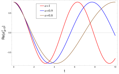
(a)

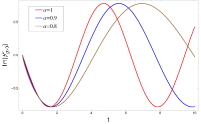
(b)

Figure 2: In the case $V\left(x\right)=0$ and $g>0$ a) Real part of the $\psi^{\alpha}_{g>0}\left(x,t\right)$ for $\alpha=1,0.9,0.8$ values, b) Imaginer part of the $\psi^{\alpha}_{g>0}\left(x,t\right)$ for $\alpha=1,0.9,0.8$ values.

As it can be seen from Figure 2 that the time evolution of the real and imaginer part of the wave function $\psi^{\alpha}_{g>0}\left(x,t\right)$ clearly depend on the fractional parameter $\alpha$. For small values of the time, wave function solution depend on time nearly coincident for different $\alpha$ values, however fractional parameter $\alpha$ values substantially affect the solution of $\psi^{\alpha}_{g>0}\left(x,t\right)$ when time is increased. Indeed for $\alpha<1$ values this effect can be clearly seen in Figure 2 (a) and (b) at large time values.

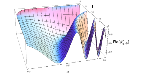
Figure 3: Time and fractional parameter $\alpha$ dependence of the real part of $\psi^{\alpha}_{g>0}\left(x,t\right)$ for $V\left(x\right)=0$ and $g>0$.

On the other hand to see effect of the fractional parameter on the ground state dynamics of condensation of bosonic particles with fractality, we give the surface plot in Figure 3. This figure clearly shows that the real part of the wave function $\psi^{\alpha}_{g>0}\left(x,t\right)$ evolutes to make oscillation with time for arbitrary $\alpha$ values, however, for in the limit $\alpha\rightarrow 0$, at the same time, or in the limit $t\rightarrow 0$ the wave function $\psi^{\alpha}_{g>0}\left(x,t\right)$ goes to stationary state which means that the wave function in these limit does not change. Hence in these limit values, stationary solution of the time-fractional GP equation is independent of time. For this reason, the soliton solution of time fractional GP equation (16) in these limit is stable similar to soliton solution of GP equation (1). The same behavior appears in imaginer part of the the wave function $\psi^{\alpha}_{g>0}\left(x,t\right)$ .

Example 2

Secondly we consider GP equation of integer and fractional order for $V\left(x\right)=0$ and attractive interaction $g=-1<0$. Hence we will discuss GPE of integer order in 2.Case-I and GPE of fractional order in 2.Case-II.

2.Case-I

For $V\left(x\right)=0$ and attractive interaction $g=-1<0$, the iterative equation (53) is given as

$$\phi_{j}=\frac{i}{\hbar}\int_{0}^{t}\left(\frac{\hbar}{2m}\nabla^{2}\phi_{j-1}-g\sum_{i=0}^{j-1}\sum_{k=0}^{j-i-1}\left|\phi_{i}\right|\left|\phi_{k}\right|\phi_{j-k-1}\right)dt\ .$$ (89)

In this case, the HPM solutions of $\phi_{j}$ are given by

$$\phi_{0}=\sec hx$$ (90)

$$\phi_{1}=-\frac{it}{2\Gamma\left(2\right)}\sec hx$$ (91)

$$\phi_{2}=-\frac{t^{2}}{3\Gamma\left(3\right)}\sec hx$$ (92)

$$\phi_{3}=\frac{it^{3}}{4\Gamma\left(4\right)}\sec hx$$ (93)

$$\begin{array}[]{c}.\\ .\\ .\end{array}$$ (94)

$$\phi_{n}=\left(-1\right)^{n}\frac{\left(it\right)^{n}}{(n+1)\Gamma\left(n+1\right)}\sec hx$$ (95)

where we set $\hbar=m=1$ for simplicity. Using the series expansion

$$\psi\left(x,t\right)=\phi_{0}\left(x\right)+p\phi_{1}\left(x\right)+p^{2}\phi_{2}\left(x\right)+...=\sum_{j=0}^{\infty}p^{j}\phi_{j}\left(x\right)$$ (96)

the final results can be written as

$$\psi_{g<0}\left(x,t\right)=\sec hx+\sum_{n=1}^{\infty}\left(-1\right)^{n}\frac{\left(it\right)^{n}}{(n+1)\Gamma\left(n+1\right)}\sec hx\ .$$ (97)

This solution can be defined Mittag-Leffler function for $\alpha=1$ as

$$\psi_{g<0}\left(x,t\right)\cong E_{1}\left[-\left(\frac{t}{\tau}\right)\right]\sec hx=\sec hxe^{-t/\tau}$$ (98)

where $i=1/\tau$. This unnormalized solution is of the same analytical form with Eq. (13) which corresponds bright soliton solution of GP equation. The numerical demonstration of the Eq. (100) for $t=0$ and the probability density of $\psi_{g<0}\left(x,t\right)$ are given is given in Figs. (4a) and (4b), respectively. As it can be seen from Fig. (4b) when external potential $V\left(x\right)=0$, the probability density for attractive interactions has bright soliton form. These results confirm that obtained solution using HPM is the same with analytical solution of GP equation of integer order for $V\left(x\right)=0$ and $g<0$.

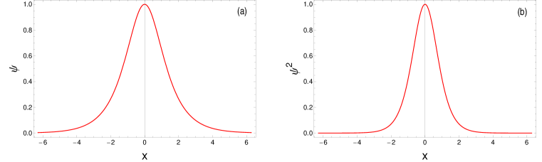
Figure 4: In the case $V\left(x\right)=0$ and $g<0$ a) Numerical representation of the $\psi_{g<0}\left(x,0\right)$, b) Numerical representation of the probability density of $\psi_{g<0}\left(x,t\right)$.

2.Case-II

Now we consider time-fractional GP equation for $V\left(x\right)=0$ and $g=-1<0$, The iterative equation (66) of the time-fractional GP equation for $V\left(x\right)=0$

$$\phi_{j}^{\alpha}=\frac{i}{\hbar\Gamma\left(\alpha\right)}\int_{0}^{t}\left(t-\tau\right)^{\alpha-1}\left(\frac{\hbar}{2m}\nabla^{2}\phi_{j-1}^{\alpha}-g\sum_{i=0}^{j-1}\sum_{k=0}^{j-i-1}\left|\phi_{i}^{\alpha}\right|\left|\phi_{k}^{\alpha}\right|\phi_{j-k-1}^{\alpha}\right)d\tau\ .$$ (99)

For attractive interaction, the HPM solutions of $\phi_{j}^{\alpha}$ are given by

$$\phi_{0}^{\alpha}=\sec hx$$ (100)

$$\phi_{1}^{\alpha}=-\frac{it^{\alpha}}{\Gamma\left(\alpha+2\right)}\sec hx$$ (101)

$$\phi_{2}^{\alpha}=-\frac{t^{2\alpha}}{\Gamma\left(2\alpha+2\right)}\sec hx$$ (102)

$$\phi_{3}^{\alpha}=\frac{it^{3\alpha}}{\Gamma\left(3\alpha+2\right)}\sec hx$$ (103)

$$\begin{array}[]{c}.\\ .\\ .\end{array}$$ (104)

$$\phi_{n}^{\alpha}=\left(-1\right)^{n}\frac{\left(it^{\alpha}\right)^{n}}{\Gamma\left(n\alpha+2\right)}\sec hx$$ (105)

where we set $\hbar=m=1$ for simplicity. All solutions can be added in series expansion as

$$\psi^{\alpha}\left(x,t\right)=\phi_{0}^{\alpha}\left(x\right)+p\phi_{1}^{\alpha}\left(x\right)+p^{2}\phi_{2}^{\alpha}\left(x\right)+...=\sum_{j=0}^{\infty}p^{j}\phi_{j}^{\alpha}\left(x\right)\ .$$ (106)

This produces the final results for $g<0$

$$\psi_{g<0}^{\alpha}\left(x,t\right)=\sec hx+\sum_{n=1}^{\infty}\left(-1\right)^{n}\frac{\left(it^{\alpha}\right)^{n}}{\Gamma\left(n\alpha+2\right)}\sec hx\ .$$ (107)

This solution can be written in terms of Mittag-Leffler function as

$$\psi_{g<0}^{\alpha}\left(x,t\right)=\sec hx+\sum_{n=1}^{\infty}\frac{\left(-\left(t/\tau\right)^{\alpha}\right)^{n}}{(n\alpha+1)\Gamma\left(n\alpha+1\right)}\sec hx\cong E_{\alpha}\left(-\left(t/\tau\right)^{\alpha}\right)\sec hx$$ (108)

where we set $i=1/\tau^{\alpha}$. According to Eqs. (31) and (32) the asymptotic behavior of the Mittag-Leffler function, the fractional solution (110) is given by stretched exponential form

$$\psi_{g<0}^{\alpha}\left(x,t\right)\cong E_{\alpha}\left(-\left(t/\tau\right)^{\alpha}\right)\sec hx\sim\exp\left(-\frac{\left(t/\tau\right)^{\alpha}}{\Gamma\left(\alpha+1\right)}\right)\sec hx$$ (109)

or for long-time regime is given by inverse power-law as

$$\psi_{g<0}^{\alpha}\left(x,t\right)\cong E_{\alpha}\left(-\left(t/\tau\right)^{\alpha}\right)\sec hx\sim\left(\frac{t}{\tau}\right)^{\alpha}\frac{1}{\Gamma\left(1-\alpha\right)}\sec hx\ .$$ (110)

The nice analytical results are solutions of the time-fractional GP equation for $V\left(x\right)=0$ and $g=-1<0$. It can be clearly seen from Eqs. (111) and (112) that the time-dependent solution of time-fractional GP equation (16) is different from standard GP equation (1). Indeed, solutions (111) and (112) of time-fractional GP equation indicate that the ground state dynamics of the Bose-Einstein condensation evolute with time in complex space as obey to stretched exponential for short time regime and power law for long-time regime in the case external potential zero and interactions between bosonic particles are attractive. Whereas for the same case i.e. $V\left(x\right)=0$ and $g=-1<0$ the ground state dynamics of the condensation exponentially evolutes with time. However, the spatial part of both solution in Eq. (110) and in Eq. (100) are equal. Therefore, it is excepted that the time-fractional dynamics of condensation also produces bright soliton behavior similar to Eq. (100) as it can be seen in Fig. (4b). On the other hand, here we must remark that the fractional parameter $\alpha$ is a measure of fractality in between particles in condensation progress. Hence it determine time evolution of the ground state dynamics of condensation.

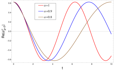
(a)

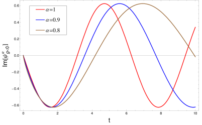
(b)

Figure 5: In the case $V\left(x\right)=0$ and $g<0$ a) Real part of the $\psi^{\alpha}_{g<0}\left(x,t\right)$ for $\alpha=1,0.9,0.8$ values, b) Imaginer part of the $\psi^{\alpha}_{g<0}\left(x,t\right)$ for $\alpha=1,0.9,0.8$ values.

In order to demonstrate the effect of the fractional parameter on the ground state dynamics or another say to investigate ground state dynamics of fractional condensation we plot the real and imaginer part of the $\psi^{\alpha}_{g<0}\left(x,t\right)$ for several $\alpha$ values.

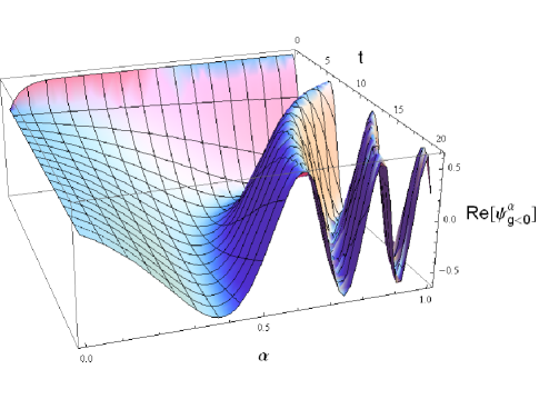
Figure 6: Time and fractional parameter $\alpha$ dependence of the real part of $\psi^{\alpha}_{g<0}\left(x,t\right)$ for $V\left(x\right)=0$ and $g<0$.

As it can be seen from Figure 5 that the time evolution of the real and imaginer part of the wave function $\psi^{\alpha}_{g<0}\left(x,t\right)$ clearly depend on fractional parameter $\alpha$. For small values of the time, wave function solution depend on time nearly coincident for different $\alpha$ values, however fractional parameter $\alpha$ values substantially affect the solution of $\psi^{\alpha}_{g<0}\left(x,t\right)$ when time is increased. Indeed for $\alpha<1$ values this effect can be clearly seen in Figure 5 (a) and (b) at large time values. Furthermore, to see effect of the fractional parameter on the ground state dynamics of condensation of bosonic particles, we give the surface plot in Figure 6. This figure clearly shows that the real part of the wave function $\psi^{\alpha}_{g<0}\left(x,t\right)$ evolutes to make oscillation with time for arbitrary $\alpha$ values, however, for in the limit $\alpha\rightarrow 0$, at the same time, or in the limit $t\rightarrow 0$ the wave function $\psi^{\alpha}_{g<0}\left(x,t\right)$ goes to stationary state which means that the wave function in these limit does not change. Hence in these limit values, stationary solution of the time-fractional GP equation is independent of time. For this reason, the soliton solution of time fractional GP equation (16) in these limit is stable similar to soliton solution of GP equation (1). The same behavior appears in imaginer part of the the wave function $\psi^{\alpha}_{g<0}\left(x,t\right)$.

Example 3

Thirdly, in this example, by using HPM we will obtain solutions of the GP equation of integer and fractional order for optical lattice potential $V\left(x\right)=\sin^{2}x$ and repulsive interaction i.e. $g=1>0$. Hence we will consider GPE of integer order in 3.Case-I and GPE of fractional order in 3.Case-II. We note that we have found the analytical solution of GP equation as $\psi_{g=1}\left(x,t\right)=e^{-3it/2}\cos x$ in the case $g=1>0$ for optical lattice potential $V\left(x\right)=\sin^{2}x$ which satisfy Eq. (1).

3.Case-I

For optical lattice potential $V\left(x\right)=\sin^{2}x$ and repulsive interaction $g=1>0$, the iterative equation (53) is given as

$$\phi_{j}=\frac{i}{\hbar}\int_{0}^{t}\left(\frac{\hbar}{2m}\nabla^{2}\phi_{j-1}-\sin^{2}x\phi_{j-1}-g\sum_{i=0}^{j-1}\sum_{k=0}^{j-i-1}\left|\phi_{i}\right|\left|\phi_{k}\right|\phi_{j-k-1}\right)d\tau$$ (111)

For this potential, the HPM solutions of $\phi_{j}$ are given by

$$\phi_{0}=\cos x$$ (112)

$$\phi_{1}=-\frac{3it}{2\Gamma\left(2\right)}\cos x$$ (113)

$$\phi_{2}=-\frac{9t^{2}}{4\Gamma\left(3\right)}\cos x$$ (114)

$$\phi_{3}=\frac{27it^{3}}{8\Gamma\left(4\right)}\cos x$$ (115)

$$\begin{array}[]{c}.\\ .\\ .\end{array}$$ (116)

$$\phi_{n}=\left(-1\right)^{n}\frac{\left(3it\right)^{n}}{2^{n}\Gamma\left(n+1\right)}\cos x$$ (117)

where we set $\hbar=m=1$ for simplicity. If these $\phi_{j}$ terms can be put in the series

$$\psi\left(x,t\right)=\phi_{0}\left(x\right)+p\phi_{1}\left(x\right)+p^{2}\phi_{2}\left(x\right)+...=\sum_{j=0}^{\infty}p^{j}\phi_{j}\left(x\right)$$ (118)

we obtain final results for $g=1>0$

$$\psi_{g>0}\left(x,t\right)=\cos x+\sum_{n=1}^{\infty}\left(-1\right)^{n}\frac{\left(3it\right)^{n}}{2^{n}\Gamma\left(n+1\right)}\cos x\ .$$ (119)

The solution (121) can be written in terms of Mittag-Leffler function for $\alpha=1$ as

$$\psi_{g>0}\left(x,t\right)=\cos x+\sum_{n=1}^{\infty}\frac{\left(-\left(t/\tau\right)\right)^{n}}{\Gamma\left(n+1\right)}\cos x=E_{1}\left(-\left(t/\tau\right)\right)\cos x$$ (120)

where we set $3i/2=1/\tau$. Eq. (122) can be given in exponential form as

$$\psi_{g>0}\left(x,t\right)=E_{1}\left(-\left(t/\tau\right)\right)\cos x=e^{-t/\tau}\cos x\ .$$ (121)

Our analytical result in Eq. (123) is the same with analytical solution of GP equation for optical lattice potential $V\left(x\right)=\sin^{2}x$ and attractive interactions $g>0$. The numerical demonstrations of the Eq. (123) for $t=0$ and the probability density of $\psi_{g>0}\left(x,t\right)$ are given is given in Figs. (7a) and (7b), respectively. As it can be seen from Fig. (7a) that the solution $\psi_{g>0}\left(x,t\right)$ for $t=0$ has a Gaussian form, whereas probability density of $\psi_{g>0}\left(x,t\right)$ has a double well shape for optical lattice potential $V\left(x\right)=\sin^{2}x$ and attractive interactions $g=1>0$. As a result we note that these analytical and numerical results confirm that obtained solution using HPM is the same with analytical solution of GP equation of integer order for $V\left(x\right)=\sin^{2}x$ and $g=1>0$.

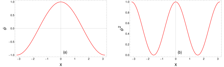
Figure 7: $V\left(x\right)=\sin^{2}x$ and repulsive interactions $g=1>0$, a) Numerical representation of the $\psi_{g>0}\left(x,0\right)$, b) Numerical representation of the probability density of $\psi_{g>0}\left(x,t\right)$.

3.Case-II

Now we consider time-fractional GP equation for $V\left(x\right)=\sin^{2}x$ and repulsive interaction $g=1>0$. The iterative equation (66) of the time-fractional GP equation for this potential is given by

$$\phi_{j}^{\alpha}=\frac{i}{\hbar\Gamma\left(\alpha\right)}\int_{0}^{t}\left(t-\tau\right)^{\alpha-1}\left(\frac{\hbar}{2m}\nabla^{2}\phi_{j-1}^{\alpha}-\sin^{2}x\phi_{j-1}^{\alpha}-g\sum_{i=0}^{j-1}\sum_{k=0}^{j-i-1}\left|\phi_{i}^{\alpha}\right|\left|\phi_{k}^{\alpha}\right|\phi_{j-k-1}^{\alpha}\right)d\tau$$ (122)

For $g=1>0$, the HPM solutions of $\phi_{j}^{\alpha}$ are given by

$$\phi_{0}^{\alpha}=\cos x$$ (123)

$$\phi_{1}^{\alpha}=-\frac{3it^{\alpha}}{2\Gamma\left(\alpha+1\right)}\cos x$$ (124)

$$\phi_{2}^{\alpha}=-\frac{9t^{2\alpha}}{4\Gamma\left(2\alpha+1\right)}\cos x$$ (125)

$$\phi_{3}^{\alpha}=\frac{27it^{3\alpha}}{8\Gamma\left(3\alpha+1\right)}\cos x$$ (126)

$$\begin{array}[]{c}.\\ .\\ .\end{array}$$ (127)

$$\phi_{n}^{\alpha}=\left(-1\right)^{n}\frac{\left(3it^{\alpha}\right)^{n}}{2^{n}\Gamma\left(n\alpha+1\right)}\cos x$$ (128)

where we set $\hbar=m=1$ for simplicity. These terms can be put in a seises to obtain $\psi^{\alpha}\left(x,t\right)$

$$\psi^{\alpha}\left(x,t\right)=\phi_{0}^{\alpha}\left(x\right)+p\phi_{1}^{\alpha}\left(x\right)+p^{2}\phi_{2}^{\alpha}\left(x\right)+...=\sum_{j=0}^{\infty}p^{j}\phi_{j}^{\alpha}\left(x\right)$$ (129)

We obtain final results for $g=1>0$

$$\psi_{g>0}^{\alpha}\left(x,t\right)=\cos x+\sum_{n=1}^{\infty}\left(-1\right)^{n}\frac{\left(3it^{\alpha}\right)^{n}}{2^{n}\Gamma\left(n\alpha+1\right)}\cos x\ .$$ (130)

This solution can be written in terms of Mittag-Leffler function as

$$\psi_{g>0}^{\alpha}\left(x,t\right)=\cos x+\sum_{n=1}^{\infty}\frac{\left(-\left(t/\tau\right)^{\alpha}\right)^{n}}{\Gamma\left(n\alpha+1\right)}\cos x=E_{\alpha}\left(-\left(t/\tau\right)^{\alpha}\right)\cos x$$ (131)

where we set $3i/2=1/\tau^{\alpha}$. According to Eqs. (31) and (32) the asymptotic behavior of the Mittag-Leffler function, the fractional solution (133) is given by stretched exponential form

$$\psi_{g>0}^{\alpha}\left(x,t\right)=E_{\alpha}\left(-\left(t/\tau\right)^{\alpha}\right)\cos x\sim\exp\left(-\frac{\left(t/\tau\right)^{\alpha}}{\Gamma\left(\alpha+1\right)}\right)\cos x$$ (132)

or for long-time regime is given by inverse power-law as

$$\psi_{g>0}^{\alpha}\left(x,t\right)=E_{\alpha}\left(-\left(t/\tau\right)^{\alpha}\right)\cos x\sim\left(\frac{t}{\tau}\right)^{\alpha}\frac{1}{\Gamma\left(1-\alpha\right)}\cos x\ .$$ (133)

Eqs. (134) and (135) are solutions of the time-fractional GP equation for $V\left(x\right)=\sin^{2}x$ and $g=1>0$. It can be clearly seen from Eqs. (134) and (135) that the time-dependent solution of time-fractional GP equation (16) is different from standard GP equation (1). Indeed, solutions (134) and (135) of time-fractional GP equation indicate that for $\alpha<1$ the ground state dynamics of the Bose-Einstein condensation evolute with time in complex space as obey to stretched exponential for short time regime and power law for long-time regime in the case external potential $V\left(x\right)=\sin^{2}x$ and interactions between bosonic particles are repulsive. Whereas for the $\alpha=1$, the ground state dynamics of the condensation exponentially evolutes with time. However, the spatial part of both solution in Eq. (133) and in Eq. (123) are equal. Therefore, it is excepted that the time-fractional dynamics of condensation also produces double well shape behavior similar to Eq. (135) as it can be seen in Fig. (7b). On the other hand, here we must remark that the fractional parameter $\alpha$ is a measure of fractality in between particles in condensation progress. Hence it determine time evolution of the ground state dynamics of condensation.

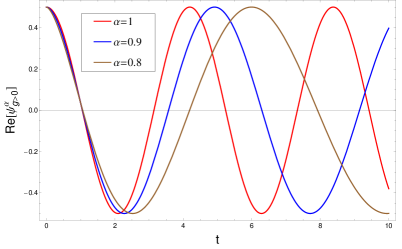
(a)

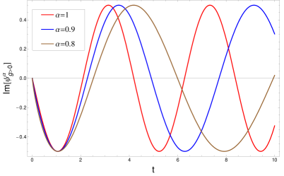
(b)

Figure 8: In the case $V\left(x\right)=\sin^{2}x$ and $g>0$ a) Real part of the $\psi^{\alpha}_{g>0}\left(x,t\right)$ for $\alpha=1,0.9,0.8$ values, b) Imaginer part of the $\psi^{\alpha}_{g>0}\left(x,t\right)$ for $\alpha=1,0.9,0.8$ values.

In order to demonstrate effect of the fractional parameter on the ground state dynamics or another say to investigate ground state dynamics of condensation with fractality we plot the real and imaginer part of the $\psi^{\alpha}_{g>0}\left(x,t\right)$ for several $\alpha$ values.

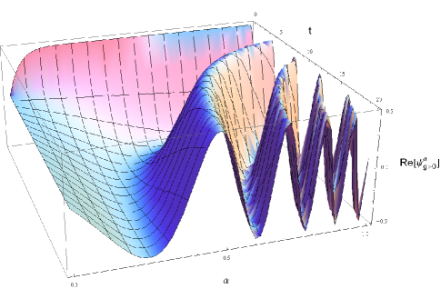
Figure 9: Time and fractional parameter $\alpha$ dependence of the real part of $\psi^{\alpha}_{g>0}\left(x,t\right)$ for $V\left(x\right)=\sin^{2}x$ and $g>0$.

As it can be seen from Figure 8 that the time evolution of the real and imaginer part of the wave function $\psi^{\alpha}_{g>0}\left(x,t\right)$ clearly depend on fractional parameter $\alpha$. For small values of the time, wave function solution depend on time nearly coincident for different $\alpha$ values, however fractional parameter $\alpha$ values substantially affect the solution of $\psi^{\alpha}_{g>0}\left(x,t\right)$ when time is increased. Indeed for $\alpha<1$ values this effect can be clearly seen in Figure 8 (a) and (b) at large time values. Furthermore, to see effect of the fractional parameter on the ground state dynamics of condensation of bosonic particles with fractality, we give the surface plot in Figure 9. This figure clearly shows that the real part of the wave function $\psi^{\alpha}_{g>0}\left(x,t\right)$ evolutes to make oscillation with time for arbitrary $\alpha$ values, however, for in the limit $\alpha\rightarrow 0$, at the same time, or in the limit $t\rightarrow 0$ the wave function $\psi^{\alpha}_{g>0}\left(x,t\right)$ goes to stationary state which means that the wave function in these limit does not change. Hence in these limit values, stationary solution of the time-fractional GP equation is independent of time.

Example 4

Finally, we will obtain solutions of the GP equation of integer and fractional order for optical lattice potential $V\left(x\right)=-\sin^{2}x$ and attractive interaction i.e. $g=-1<0$. Hence we will consider GPE of integer order in 4.Case-I and GPE of fractional order in 4.Case-II. We note that we have found the analytical solution of GP equation as $\psi_{g=-1}\left(x,t\right)=e^{it/2}\cos x$ in the case $g=-1<0$ for optical lattice potential $V\left(x\right)=-\sin^{2}x$ which satisfy Eq. (1).

4.Case-I

For optical lattice potential $V\left(x\right)=-\sin^{2}x$ and attractive interaction $g=-1<0$, the iterative relation (53) is written as

$$\phi_{j}=\frac{i}{\hbar}\int_{0}^{t}\left(\frac{\hbar}{2m}\nabla^{2}\phi_{j-1}+\sin^{2}x\phi_{j-1}-g\sum_{i=0}^{j-1}\sum_{k=0}^{j-i-1}\left|\phi_{i}\right|\left|\phi_{k}\right|\phi_{j-k-1}\right)d\tau$$ (134)

For this potential, the HPM solutions of $\phi_{j}$ are given by

$$\phi_{0}=\cos x$$ (135)

$$\phi_{1}=-\frac{it}{2\Gamma\left(1\right)}\cos x$$ (136)

$$\phi_{2}=-\frac{t^{2}}{4\Gamma\left(3\right)}\cos x$$ (137)

$$\phi_{3}=-\frac{it^{3}}{8\Gamma\left(4\right)}\cos x$$ (138)

$$\begin{array}[]{c}.\\ .\\ .\end{array}$$ (139)

$$\phi_{n}=\left(-1\right)^{n}\frac{\left(it\right)^{n}}{2^{n}\Gamma\left(n+1\right)}\cos x$$ (140)

where we set $\hbar=m=1$ for simplicity. If these terms are put in the series

$$\psi\left(x,t\right)=\phi_{0}\left(x\right)+p\phi_{1}\left(x\right)+p^{2}\phi_{2}\left(x\right)+...=\sum_{j=0}^{\infty}p^{j}\phi_{j}\left(x\right)$$ (141)

we obtain final results as

$$\psi_{g<0}\left(x,t\right)=\cos x+\sum_{n=1}^{\infty}\left(-1\right)^{n}\frac{\left(it\right)^{n}}{2^{n}\Gamma\left(n+1\right)}\cos x\ .$$ (142)

The solution (144) can be written in terms of Mittag-Leffler function for $\alpha=1$ as

$$\psi_{g<0}\left(x,t\right)=\cos x+\sum_{n=1}^{\infty}\frac{\left(-\left(t/\tau\right)\right)^{n}}{\Gamma\left(n\alpha+1\right)}\cos x=E_{1}\left(-\left(t/\tau\right)\right)\cos x$$ (143)

where we set $i/2=1/\tau$. Eq. (145) can be given in exponential form as

$$\psi_{g<0}\left(x,t\right)=E_{1}\left(-\left(t/\tau\right)\right)\cos x=e^{-t/\tau}\cos x\ .$$ (144)

Figure 10: $V\left(x\right)=-\sin^{2}x$ and attractive interactions $g=-1<0$, a) Numerical representation of the $\psi_{g<0}\left(x,0\right)$, b) Numerical representation of the probability density of $\psi_{g<0}\left(x,t\right)$.

Our HPM result in Eq. (146) is the same with analytical solution of GP equation for optical lattice potential $V\left(x\right)=-\sin^{2}x$ and attractive interactions $g<0$. At $t=0$, the numerical demonstrations of the $\psi_{g<0}\left(x,0\right)$ and the probability density of $\psi_{g<0}\left(x,0\right)$ are given is given in Figs. (10a) and (10b), respectively. As it can be seen from Fig. (7a) that the solution $\psi_{g<0}\left(x,0\right)$ for $t=0$ has a Gaussian form, whereas probability density of $\psi_{g<0}\left(x,t\right)$ has a double well shape for optical lattice potential $V\left(x\right)=-\sin^{2}x$ and attractive interactions $g=-1<0$. As a result we note that these analytical and numerical results confirm that obtained solution using HPM is the same with analytical solution of GP equation of integer order for $V\left(x\right)=-\sin^{2}x$ and $g=-1<0$.

4.Case-II

In last case, we will consider time-fractional GP equation for optical lattica potential $V\left(x\right)=-\sin^{2}x$ and attractive interaction $g=-1<0$. The iterative equation (66) of the time-fractional GP equation for this potential is given by

$$\phi_{j}^{\alpha}=\frac{i}{\hbar\Gamma\left(\alpha\right)}\int_{0}^{t}\left(t-\tau\right)^{\alpha-1}\left(\frac{\hbar}{2m}\nabla^{2}\phi_{j-1}^{\alpha}+\sin^{2}x\phi_{j-1}^{\alpha}-g\sum_{i=0}^{j-1}\sum_{k=0}^{j-i-1}\left|\phi_{i}^{\alpha}\right|\left|\phi_{k}^{\alpha}\right|\phi_{j-k-1}^{\alpha}\right)d\tau$$ (145)

For this potential, the HPM solutions of $\phi_{j}$ are given by

$$\phi_{0}^{\alpha}=\cos x$$ (146)

$$\phi_{1}^{\alpha}=-\frac{it^{\alpha}}{2\Gamma\left(\alpha+1\right)}\cos x$$ (147)

$$\phi_{2}^{\alpha}=-\frac{t^{2\alpha}}{4\Gamma\left(2\alpha+1\right)}\cos x$$ (148)

$$\phi_{3}^{\alpha}=-\frac{it^{3\alpha}}{8\Gamma\left(3\alpha+1\right)}\cos x$$ (149)

$$\begin{array}[]{c}.\\ .\\ .\end{array}$$ (150)

$$\phi_{n}^{\alpha}=\left(-1\right)^{n}\frac{\left(it^{\alpha}\right)^{n}}{2^{n}\Gamma\left(n\alpha+1\right)}\cos x$$ (151)

where we set $\hbar=m=1$ for simplicity. If these terms are put in the series

$$\psi^{\alpha}_{g<0}\left(x,t\right)=\phi_{0}^{\alpha}\left(x\right)+p\phi_{1}^{\alpha}\left(x\right)+p^{2}\phi_{2}^{\alpha}\left(x\right)+...=\sum_{j=0}^{\infty}p^{j}\phi_{j}^{\alpha}\left(x\right)$$ (152)

we obtain final results as

$$\psi_{g<0}^{\alpha}\left(x,t\right)=\cos x+\sum_{n=1}^{\infty}\left(-1\right)^{n}\frac{\left(it^{\alpha}\right)^{n}}{2^{n}\Gamma\left(n\alpha+1\right)}\cos x\ .$$ (153)

This solution can be written in terms of Mittag-Leffler function as

$$\psi_{g<0}^{\alpha}\left(x,t\right)=\cos x+\sum_{n=1}^{\infty}\frac{\left(-\left(t/\tau\right)^{\alpha}\right)^{n}}{\Gamma\left(n\alpha+1\right)}\cos x=E_{\alpha}\left(-\left(t/\tau\right)^{\alpha}\right)\cos x$$ (154)

where we set $i/2=1/\tau^{\alpha}$. According to Eqs. (31) and (32) the asymptotic behavior of the Mittag-Leffler function, the fractional solution (156) is given by stretched exponential form

$$\psi_{g<0}^{\alpha}\left(x,t\right)=E_{\alpha}\left(-\left(t/\tau\right)^{\alpha}\right)\cos x\sim\exp\left(-\frac{\left(t/\tau\right)^{\alpha}}{\Gamma\left(\alpha+1\right)}\right)\cos x$$ (155)

or for long-time regime is given by inverse power-law as

$$\psi_{g<0}^{\alpha}\left(x,t\right)=E_{\alpha}\left(-\left(t/\tau\right)^{\alpha}\right)\cos x\sim\left(\frac{t}{\tau}\right)^{\alpha}\frac{1}{\Gamma\left(1-\alpha\right)}\cos x\ .$$ (156)

Eqs. (157) and (158) are solutions of the time-fractional GP equation for $V\left(x\right)=-\sin^{2}x$ and $g=-1<0$. It can be clearly seen from Eqs. (157) and (158) that the time-dependent solution of time-fractional GP equation (16) is different from solution of the standard GP equation (1). Indeed, solutions (157) and (158) of time-fractional GP equation indicate that the ground state dynamics of the Bose-Einstein condensation evolute with time in complex space as obey to stretched exponential for short time regime and power law for long-time regime in the case external potential $V\left(x\right)=-\sin^{2}x$ and interactions between bosonic particles are attractive. Whereas for the $\alpha=1$, the ground state dynamics of the condensation exponentially evolutes with time. However, the spatial part of both solution in Eq. (156) and in Eq. (146) are equal. Therefore, it is excepted that the time-fractional dynamics of condensation also produces double well shape behavior similar to Eq. (146) as it can be seen in Fig. (10b). On the other hand, here we must remark that the fractional parameter $\alpha$ is a measure of fractality in between particles in condensation progress. Hence it determine time evolution of the ground state dynamics of condensation.

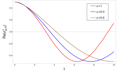
(a)

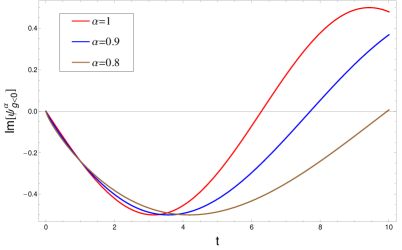
(b)

Figure 11: In the case $V\left(x\right)=-\sin^{2}x$ and $g>0$ a) Real part of the $\psi^{\alpha}_{g<0}\left(x,t\right)$ for $\alpha=1,0.9,0.8$ values, b) Imaginer part of the $\psi^{\alpha}_{g<0}\left(x,t\right)$ for $\alpha=1,0.9,0.8$ values.

In order to demonstrate effect of the fractional parameter on the ground state dynamics or another say to investigate ground state dynamics of condensation with fractality we plot the real and imaginer part of the $\psi^{\alpha}_{g<0}\left(x,t\right)$ for several $\alpha$ values.

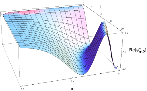
Figure 12: Time and fractional parameter $\alpha$ dependence of the real part of $\psi^{\alpha}_{g<0}\left(x,t\right)$ for $V\left(x\right)=-\sin^{2}x$ and $g<0$.

As it can be seen from Figure 11 that the time evolution of the real and imaginer part of the wave function $\psi^{\alpha}_{g<0}\left(x,t\right)$ clearly depend on fractional parameter $\alpha$. For small values of the time, wave function solution depend on time nearly coincident for different $\alpha$ values, however fractional parameter $\alpha$ values substantially affect the solution of $\psi^{\alpha}_{g<0}\left(x,t\right)$ when time is increased. Indeed for $\alpha<1$ values this effect can be clearly seen in Figure 11 (a) and (b) at large time values. Furthermore, to see effect of the fractional parameter $\alpha$ on the ground state dynamics of condensation of bosonic particles, we give the surface plot in Figure 12. This figure clearly shows that the real part of the wave function $\psi^{\alpha}_{g<0}\left(x,t\right)$ evolutes to make oscillation with time for arbitrary $\alpha$ values, however, for in the limit $\alpha\rightarrow 0$, at the same time, or in the limit $t\rightarrow 0$ the wave function $\psi^{\alpha}_{g<0}\left(x,t\right)$ goes to stationary state which means that the wave function in these limit does not change. Hence in these limit values, stationary solution of the time-fractional GP equation is independent of time.

8 Conclusion

In this study, we have suggested fractional Gross-Pitaevskii equations to investigate the time-dependent ground state dynamics of the Bose-Einstein condensation of weakly interacting bosonic particle system which can includes non-Markovian processes or non-Gaussian distributions and long-range interactions. However we focused the time-fractional Gross-Pitaevskii equation and obtained solutions of the the Gross-Pitaevskii equation of the integer and fractional order for repulsive and attractive interactions in the case external trap potentials $V(x)=0$ and optical lattice potential $V\left(x\right)=\pm\sin^{2}x$ using Homotopy Perturbation Method. Summarizing, in the Example 1 and 2, we have considered GP equation of integer and fractional order for the repulsive and attractive interactions in the case external trap potential $V(x)=0$. On the other hand, in the Example 3 and 4, we have discussed GP equation of integer and fractional order for the repulsive and attractive interactions in the case the optical lattice potentials $V\left(x\right)=\pm\sin^{2}x$. We found several results: 1) we have shown that our HPM solutions of GP equation of integer order are the same the analytical solutions of its for $V\left(x\right)=0$ and optical lattice potentials $V\left(x\right)=\pm\sin^{2}x$. These confirms that HPM is reliable method to solve time-dependent non-linear partial differential equations as well GP equation, 2) We show that the time dependent part of the solutions of the time-fractional GP equation have stretched exponential form for repulsive and attractive interactions in the case $V\left(x\right)=0$ and optical lattice potentials $V\left(x\right)=\pm\sin^{2}x$. However, for the same potentials and interactions, time dependent part of the solution of GP equation of integer order have exponential form. These means that time evolution of the ground state dynamics of condensation of bosonic particles including non-Markovian processes deviates exponential form, and evolutes with time as stretched exponentially.

We conclude that the condensation of weakly interacting bosonic particles have non-Markovian processes which can be lead fractional dynamics in condensate phase. This dynamics can be represented by time-fractional Gross-Pitaevskii equation. Although time-fractional GP equation does not predict critical temperature $T_{c}$ of the bosonic system, it can help to understand ground state dynamic of these system. To understand the contradictions of the experimental and theoretical predictions of critical temperature about condensation in real bosonic gas, the memory effects of the non-Markovian processes, non-Gaussian distribution of particles, the long-range inter-particle interaction effects or the fractal structure of the interacting in a bosonic system below the $T_{c}$ can be taken into account. In the next study, to investigate of the condensation dynamics of weakly interacting bosonic systems we will consider the time and space-fractional GP equation for many different potentials, which have no analytical solutions. And also we will try to determine relation between condensation temperature of real bosonic system and $\alpha$ used in the fractional Gross-Pitaevskii equation.

References

References

- [1] E. P. Gross, Il Nuovo Cimento 20 454 (1961).
- [2] L. P. Pitaevskii, S. Stringari, (2003). Bose Einstein Condensation. Oxford: Clarendon Press.
- [3] Unpublished talk on the Bose-Einstein Condensation and fractional dynamics, in Dokuz Eylul University (2011).
- [4] C. J. Pethick and H. Smith, 2002 Bose Einstein Condensation in Dilute Gases (Cambridge: Cambridge University Press).
- [5] M. H. Anderson, J. R. Ensher, M. R. Matthews, C. E. Wieman and E. A. Cornell, Science 269 198 (1995).
- [6] D. S. Jin, J. R. Ensher, M. R. Matthews, C. E. Wieman and E. A. Cornell, Phys. Rev. Lett. 77 420 (1996).
- [7] K. B. Davis, M. O. Mewes, M. R. Adrews, N. J. van Druten, D. S. Durfee, D. M. Kurn and W. Ketterle, Phys. Rev. Lett. 75 3969 (1995).
- [8] M. O. Mewes, M. R. Adrews, N. J. van Druten, D. M. Kurn, D. S. Durfee and W. Ketterle, Phys. Rev. Lett. 77 416 (1996).
- [9] C.C. Bradley, C. A. Sackett, J. J. Tollett and G. Hulet, Phys. Rev. Lett. 75 1687 (1995).
- [10] V. E. Tarasov, Phys. Lett. A 336 167 (2005).
- [11] V. E. Tarasov, Ann. Phys., NY 318 286 (2005).
- [12] N. Laskin, Phys. Lett. A 268 298 (2000).
- [13] M. Naber, J. Math. Phys. 45 3339 (2004).
- [14] S. Momani, Chaos Solitons Fractals 28 930 (2006).
- [15] S. Momani, Z. Odibat, Appl. Math. Comput. 177 488 (2006).
- [16] Z. Odibat, S. Momani, Appl. Math. Comput. 181 767 (2006).
- [17] S. Momani, Z. Odibat, Chaos Solitons Fractals 31 1248 (2007).
- [18] S. Momani, Z. Odibat, Phys. Lett. A 355 271 (2006).
- [19] S. Momani, Z. Odibat, J. Comput. Appl. Math., in press.
- [20] J. H. He, Comput. Methods Appl. Mech. Engrg. 167 (1998) 57.
- [21] Z. Odibat, S. Momani, Int. J. Nonlin. Sci. Numer. Simul. 1 15 (2006).
- [22] I. Podlubny, Fractional Differential Equations, Academic Press, San Diego, CA, 1999.
- [23] A. Arikoglu, I. zkol, Chaos Solitons Fractals, in press.
- [24] Z. Odibat, S. Momani, Chaos Solitons Fractals 36 167 (2008).
- [25] S. Momani, Z. Odibat, Phys. Lett. A 365 345 (2007).
- [26] J. H. He, Comput. Methods Appl. Mech. Engrg. 178 257 (1999).
- [27] J. H. He, Int. J. Non-Linear Mech. 35 37 (2000).
- [28] M. El-Shahed, Int. J. Nonlin. Sci. Numer. Simul. 6 163 (2005).
- [29] J. H. He, Appl. Math. Comput. 151 (2004) 287.
- [30] J. H. He, Int. J. Nonlin. Sci. Numer. Simul. 6 207 (2005).
- [31] J. H. He, Phys. Lett. A 374 228 (2005).
- [32] J. H. He, Chaos Solitons Fractals 26 695 (2005).
- [33] J. H. He, Phys. Lett. A 350 87 (2006).
- [34] J. H. He, Appl. Math. Comput. 135 739 (2003).
- [35] J. H. He, Appl. Math. Comput. 156 527 (2004).
- [36] J. H. He, Appl. Math. Comput. 156 591 (2004).
- [37] J. H. He, Chaos Solitons Fractals 26 827 (2005).
- [38] A. Siddiqui, R. Mahmood, Q. Ghori, Int. J. Nonlin. Sci. Numer. Simul. 7 7 (2006).
- [39] A. Siddiqui, M. Ahmed, Q. Ghori, Int. J. Nonlin. Sci. Numer. Simul. 7 15 (2006).
- [40] J. H. He, Int. J. Mod. Phys. B 20 1141 (2006).
- [41] S. Abbasbandy, Appl. Math. Comput. 172 485 (2006).
- [42] S. Abbasbandy, Appl. Math. Comput. 173 493 (2006).
- [43] K. B. Oldham and J. Spanier, The Fractional Calculus, Academic Press, New York, NY, USA, 1974.
- [44] K. S. Miller and B. Ross, An Introduction to the Fractional Calculus and Fractional Differential Equations, John Wiley -Sons, New York, NY, USA, 1993.
- [45] S. G. Samko, A. A. Kilbas, and O. I. Marichev, Fractional Integrals and Derivatives, Gordon and Breach Science, Yverdon, Switzerland, 1993.
- [46] A. A. Kilbas, H. M. Srivastava, and J. J. Trujillo, Theory and Applications of Fractional Differential Equations, vol. 204 of North-Holland Mathematics Studies, Elsevier, Amsterdam, The Netherlands, 2006.
- [47] D. Baleanu, K. Diethelm, E. Scalas, and J. J. Trujillo, Fractional Calculus Models and Numerical Methods, World Scientific, Singapore, 2009.
- [48] I. Lakshmikantham and S. Leela, Theory of Fractional Dynamical Systems, Cambridge Scientific Publishers, Cambridge, UK, 2009.
- [49] M. Caputo, Geophys. J. R. Astr. Soc. 13 529 (1967).
- [50] G. Mittag-Leffler, Acta Math. 29 101 (1905).
- [51] A. Erdelyi (Ed.), Tables of Integral Transforms, BatemanManuscript Project, Vol. I,McGraw-Hill, New York, 1954.