A stable and adaptive semi-Lagrangian potential model for unsteady and nonlinear ship-wave interactions

Abstract

We present an innovative numerical discretization of the equations of inviscid potential flow for the simulation of three-dimensional, unsteady, and nonlinear water waves generated by a ship hull advancing in water.

The equations of motion are written in a semi-Lagrangian framework, and the resulting integro-differential equations are discretized in space via an adaptive iso-parametric collocation Boundary Element Method, and in time via implicit Backward Differentiation Formulas (BDF) with adaptive step size and variable order.

When the velocity of the advancing ship hull is non-negligible, the semi-Lagrangian formulation (also known as Arbitrary Lagrangian Eulerian formulation, or ALE) of the free-surface equations contains dominant transport terms which are stabilized with a Streamwise Upwind Petrov-Galerkin (SUPG) method.

The SUPG stabilization allows automatic and robust adaptation of the spatial discretization with unstructured quadrilateral grids. Preliminary results are presented where we compare our numerical model with experimental results on a Wigley hull advancing in calm water with fixed sink and trim.

[cor]Corresponding author, Tel.: +39 040-3787449; Fax: +39 040-3787528

1 Introduction

The use of computational tools to predict hydrodynamic performances of ships has gained a lot of popularity in recent years. Models based on potential flow theory have historically been among the most successful to assess the wave pattern around a ship hull in presence of a forward ship motion.

In this framework, the assumptions of irrotational flow and inviscid fluid reduce the Navier Stokes incompressibility constraint and momentum balance equations to the Laplace’s and Bernoulli’s equations, defined on a moving and a-priori unknown domain.

This boundary value problem is tackled with a Mixed Eulerian–Lagrangian approach, in which the Eulerian field equations are solved to obtain the fluid velocities, which are then used to displace in a Lagrangian way the free-surface, and update the corresponding potential field values tanizawa2000 . In this framework, the Eulerian problem is expressed in boundary integral form, and it is typically discretized using the Boundary Element Method (BEM). The velocity field and Bernoulli’s equation provide a kinematic boundary condition for the Lagrangian evolution of the free-surface, and a dynamic boundary condition for the evolution of the potential field.

Numerical treatment of the Lagrangian step usually relies on accurate reconstructions of the position vector and of potential field gradients. In presence of a forward motion, these reconstructions may lead to instability in the time advancing scheme for the free-surface discretization, as well as for the corresponding potential field values. A smoothing technique is often adopted to reduce the sensitivity of the discretization on the reconstruction of the full velocity field, at the cost of introducing an artificial viscosity in the system.

An alternative cure was presented by Grilli et al. grilli2001 who developed a high order iso-parametric BEM discretization of a Numerical Wave Tank to simulate overturning waves up to the breaking point on arbitrarily shaped bottoms. The use of a high order discretization bypasses the problem of reconstructing the gradients, and is very reliable when the numerical evolution of the free-surface is done in a purely Lagrangian way.

Ship hydrodynamics simulations, however, are typically carried out in a frame of reference attached to the boat, requiring the presence of a water current in the simulations. In this case a fully Lagrangian approach leads to downstream transportation of the free-surface nodes, or to their clustering around stagnation points, ultimately resulting in blowup of the simulations (see, for example, scorpioPhD ).

Beck beck1994 proposed alternative semi-Lagrangian free surface boundary conditions, under the assumption that the surface elevation function is single-valued. Employing such conditions, it is possible to prescribe arbitrarily the horizontal velocity of the free surface nodes, while preserving the physical shape of the free-surface itself.

However, if there is a significant difference between the water current speed and the horizontal nodes speed, stability issues may arise scorpioPhD , RyuKimLynett2003 . For this reason, the semi-Lagrangian free-surface boundary conditions proposed by Beck have been in most cases employed imposing nodes longitudinal speeds equal to the water current ones scorpioPhD , thus reducing the instability at the cost of more complex algorithms for mesh management.

More recently, Sung and Grilli SungGrilli2008 applied an alternative method, combining semi-Lagrangian and Lagrangian free surface boundary conditions to the problem of a pressure perturbation moving on the water surface. The semi-Lagrangian free-surface boundary conditions were used also in the work of Kjellberg, Contento and Jansson KjelContJans-2011 , where free-surface instabilities are avoided by choosing an earth-fixed reference frame, in which no current speed is needed. The drawback of this choice is that in such frame the ship moves with a specified horizontal speed, and the computational grid needs to be constantly regenerated to cover the region surrounding the hull with an adequate number of cells.

The purpose of this work is to present a new stabilized semi-Lagrangian potential model for the simulation of three dimensional unsteady nonlinear water waves generated by a ship hull advancing in calm water. The resulting integro-differential boundary value problem is discretized to a system of nonlinear differential-algebraic equations, in which the unknowns are the positions of the nodes of the computational grid, along with the corresponding values of the potential and of its normal derivative.

Time advancing of the nonlinear differential-algebraic system is performed using implicit Backward Differentiation Formulas (BDF) with variable step size and variable order, implemented in the framework of the open source library SUNDIALS sundials2005 . The collocated and iso-parametric BEM discretization of the Laplace’s equation has been implemented using the open source C++ library deal.II BangerthHartmannKanschat2007 .

The computational grid, composed by quadrilateral cells of arbitrary order, is adapted in a geometrically consistent way (see BonitoNochettoPauletti-2010-a ) via an a-posteriori error estimator based on the jump of the solution gradient along the cell internal boundaries. Even when low order boundary elements are used, accurate estimations of the position vector and potential gradients on the free-surface are recovered by a Streamwise Upwind Petrov–Galerkin (SUPG) projection, which is used to stabilize the transport dominated terms. The SUPG projection is strongly consistent, and does not introduce numerical dissipation in the equations. This allows the use of robust unstructured grids, which can be generated and managed on arbitrary hull geometries in a relatively simple way.

The test case considered in this paper is that of a Wigley hull advancing at constant speed in calm water. The simulations have been performed using bilinear elements. The arbitrary horizontal velocity specified in the semi-Lagrangian free-surface boundary condition is chosen so the nodes have null longitudinal velocity with respect to the hull. The numerical results obtained imposing six different Froude numbers are finally compared with experimental results reported in mccarthy1985 , to assess the accuracy of the model.

2 Three-dimensional potential model

The equations of motion that describe the velocity and pressure fields $\boldsymbol{v}$ and $p$ of a fluid region around a ship hull are the incompressible Navier–Stokes equations. Such equations, written in the moving domain $\Omega(t)\subset\mathbb{R}^{3}$ (a simply connected region of water surrounding the ship hull) read:

$$\rho\left(\frac{\partial\boldsymbol{v}}{\partial t}+\boldsymbol{v}\cdot{\boldsymbol{\nabla}}\boldsymbol{v}\right)={\boldsymbol{\nabla}}\cdot{\boldsymbol{\sigma}}+\boldsymbol{b}\qquad \text{ in }\Omega(t)$$ (1a)

$${\boldsymbol{\nabla}}\cdot\boldsymbol{v}=0 \text{ in }\Omega(t)$$ (1b)

$${\boldsymbol{\sigma}}\cdot\boldsymbol{n}=p_{a}\boldsymbol{n} \text{ on }\Gamma^{w}(t)$$ (1c)

$$\boldsymbol{v}=\boldsymbol{v}_{g} \text{ on }\Gamma(t)\setminus\Gamma^{w}(t)$$ (1d)

where $\rho$ is the (constant) fluid density, $\boldsymbol{b}$ are external body forces (typically gravity and possibly other inertial forces due to a non inertial movement of the reference frame), ${\boldsymbol{\sigma}}=-p\boldsymbol{I}+\mu({\boldsymbol{\nabla}}\boldsymbol{v}+{\boldsymbol{\nabla}}\boldsymbol{v}^{T})$ is the stress tensor for an incompressible Newtonian fluid, $\Gamma(t):=\partial\Omega(t)$ is the boundary of the region of interest, and $\boldsymbol{n}$ is the outer normal to the boundary $\Gamma(t)$. On the free-surface $\Gamma^{w}(t)$, the air is assumed to exert a constant atmospheric pressure $p_{a}$ on the underlying water, and we neglect shear stresses due to the wind. On the other boundaries of the domain, the prescribed velocity $\boldsymbol{v}_{g}$ is either equal to the ship hull velocity, or to a given velocity field (for inflow and outflow boundary conditions far away from the ship hull itself).

Equation (1a) is usually referred to as the momentum balance equation, while (1b) is referred to as the incompressibility constraint, or continuity equation.

In the flow field past a slender ship hull, vorticity is confined to the boundary layer region and to a thin wake following the boat: in these conditions, the assumption of irrotational and non viscous flow is fairly accurate. The neglected viscous effects can be recovered, if necessary, by other means such as empirical algebraic formulas, or —better— by the interface with a suitable boundary layer model.

For an irrotational and invishid flow, the velocity field $\boldsymbol{v}$ admits a representation through a scalar potential function $\Phi(\boldsymbol{x},t)$, namely

$$\boldsymbol{v}={\boldsymbol{\nabla}}\Phi\qquad\qquad\text{in}\ \ \Omega(t).$$ (2)

In this case, the equations of motion simplify to the unsteady Bernoulli equation and to the Laplace equation for the flow potential:

$$\frac{\partial\Phi}{\partial t}+\frac{1}{2}\left|{\boldsymbol{\nabla}}\Phi\right|^{2}+\frac{p-p_{a}}{\rho}+\boldsymbol{\beta}\cdot\boldsymbol{x}=C(t)\qquad \text{ in }\Omega(t)$$ (3a)

$$\Delta\Phi=0 \text{ in }\Omega(t)$$ (3b)

where $C(t)$ is an arbitrary function of time, and we have assumed that all body forces could be expressed as $\boldsymbol{b}=-{\boldsymbol{\nabla}}(\boldsymbol{\beta}\cdot\boldsymbol{x})$, i.e., they are all of potential type. This is true for gravitational body forces and for inertial body forces due to uniform accelerations along fixed directions of the frame of reference.

In this framework, the unknowns of the problem $\Phi$ and $p$ are uncoupled, and it is possible to recover the pressure by postprocessing the solution of the Poisson problem (3b) via Bernoulli’s Equation (3a).

Since arbitrary uniform variations of the potential field produce the same velocity field (i.e., ${\boldsymbol{\nabla}}(\Phi(\boldsymbol{x},t)+C(t))={\boldsymbol{\nabla}}\Phi(\boldsymbol{x},t)$), we can set $C(t)=0$, and we can combine Bernoulli equation (3a) and the dynamic boundary condition on the free-surface (1c) to obtain an evolution equation for the potential field $\Phi(\boldsymbol{x},t)$ on the free-surface $\Gamma^{w}(t)$.

The shape of the water domain $\Omega(t)$ is time-dependent and it is part of the unknowns of the problem. The free-surface $\Gamma^{w}(t)$ should move following the fluid velocity $\boldsymbol{v}$. In ship hydrodynamics, however, it is desirable to maintain the frame of reference attached to the boat, and study the problem in a domain which is neither fixed nor a material subdomain. Indeed, its evolution is not governed solely by the fluid motion, but also by the motion of the reference frame and by the motion of the stream of water. In addition, it has to comply to the free-surface boundary $\Gamma^{w}(t)$ which is the result of the dynamic boundary condition (1c).

A possible solution is to introduce an intermediate frame of reference, called Arbitrary Lagrangian Eulerian (ALE) (see, for example, formaggia2009cardiovascular and A). In the context of potential free-surface flows, this approach is also known as the semi-Lagrangian approach BeckCaoLee-1993-a ; scorpioPhD .

2.1 Perturbation potential and boundary conditions

Figure 1: The domain $\Omega(t)$ and the different regions in which its boundary $\partial\Omega(t)$ is split. The grey area behind the hull $\Gamma^{h}(t)$, is the absorbing beach portion of the free-surface region $\Gamma^{w}(t)$.

We solve Problem (3) on the region $\Omega(t)$ around the boat, and we move the local frame of reference with horizontal velocity $\boldsymbol{V}_{\text{f}}(t)$ which coincides with the horizontal boat velocity (which we assume as known). An additional horizontal water stream velocity $\boldsymbol{V}_{\text{s}}(t)$, expressed in a global (earth-fixed) reference frame is added to the problem.

Uniform accelerations of the reference frame $\boldsymbol{a}_{\text{f}}$ can be taken into account by incorporating them in the body force term

$$\boldsymbol{\beta}\cdot\boldsymbol{x}=\boldsymbol{a}_{\text{f}}\cdot\boldsymbol{x}+gz,$$ (4)

and it is convenient to split the potential $\Phi$ into the sum between a mean flow potential (due to the stream velocity and to the frame of reference velocity) and the so called perturbation potential $\phi$ due to the presence of the ship hull, namely

$$\Phi(\boldsymbol{x},t) =\big{(}\boldsymbol{V}_{\text{s}}(t)-\boldsymbol{V}_{\text{f}}(t)\big{)}\cdot\boldsymbol{x}+\phi(\boldsymbol{x},t)$$ (5a)

$$\boldsymbol{v}(\boldsymbol{x},t)={\boldsymbol{\nabla}}\Phi(\boldsymbol{x},t) =\boldsymbol{V}_{\text{s}}(t)-\boldsymbol{V}_{\text{f}}(t)+{\boldsymbol{\nabla}}\phi(\boldsymbol{x},t)$$ (5b)

$$\frac{\partial\Phi}{\partial t}(\boldsymbol{x},t) =\big{(}\boldsymbol{a}_{\text{s}}(t)-\boldsymbol{a}_{\text{f}}(t)\big{)}\cdot\boldsymbol{x}+\frac{\partial\phi}{\partial t}(\boldsymbol{x},t).$$ (5c)

The perturbation potential still satisfies Poisson equation

$$\Delta\phi=0\qquad\qquad\text{in}\ \ \Omega(t),$$ (6)

and in practice it is convenient to solve for $\phi$, and obtain the total potential $\Phi$ from equation (5).

In Figure 1 we present a sketch of the domain $\Omega(t)$, with the explicit splitting of the various parts of the boundary $\Gamma(t)$. On the boat hull surface, the non-penetration condition takes the form

$$\phi_{n}{}:={\boldsymbol{\nabla}}\phi\cdot\boldsymbol{n}=\boldsymbol{n}\cdot(\boldsymbol{V}_{\text{b}}-\boldsymbol{V}_{\text{s}})\qquad\qquad\text{on}\ \ \Gamma^{h}(t),$$ (7)

when expressed in terms of the perturbation potential and $\boldsymbol{V}_{\text{b}}$ is the (given) boat velocity.

On the —horizontal— bottom of the water basin $\Gamma^{b}$, the non penetration condition is also applied, namely

$$\phi_{n}{}=0\qquad\qquad\text{on}\ \ \Gamma^{b}(t).$$ (8)

A possible condition for the —vertical— far field boundary is the homogeneous Neumann condition

$$\phi_{n}{}=0\qquad\qquad\text{on}\ \ \Gamma^{ff}(t).$$ (9)

The most remarkable limit of such condition is the fact that it reflects wave energy back in the computational domain, thus limiting the simulation time. Different boundary conditions can be used to let the wave energy flow outside the domain. In B, we explain in detail the procedure used in our computations.

Applying the potential splitting (5) to Problem (3), and summarizing all boundary conditions, we obtain the perturbation potential formulation

$$\Delta\phi=0 \text{ in }\Omega(t)$$ (10a)

$$\frac{\partial\phi}{\partial t}+\boldsymbol{v}\cdot{\boldsymbol{\nabla}}\phi=-gz+\boldsymbol{a}_{\text{s}}\cdot\boldsymbol{x}+\frac{1}{2}|{\boldsymbol{\nabla}}\phi|^{2} -\mu\phi_{n}{}\qquad\text{ on }\Gamma^{w}(t)$$ (10b)

$$\phi(\boldsymbol{x},0)=\phi_{0}(\boldsymbol{x}) \text{ on }\Gamma^{w}(0)$$ (10c)

$$\phi_{n}{}=\boldsymbol{n}\cdot(\boldsymbol{V}_{\text{b}}-\boldsymbol{V}_{\text{s}}) \text{ on }\Gamma^{h}(t)$$ (10d)

$$\phi_{n}{}=0 \text{ on }\Gamma^{b}(t)\cup\Gamma^{ff}(t)$$ (10e)

$$\frac{D\Gamma^{w}(t)}{Dt}=\boldsymbol{v} \text{ on }\Gamma^{w}(t),$$ (10f)

where $\boldsymbol{v}=\boldsymbol{V}_{\text{s}}-\boldsymbol{V}_{\text{f}}+{\boldsymbol{\nabla}}\phi$. Equation (10f) is a kinematic boundary condition and indicates that the free-surfaces follows the velocity of the fluid, while Equation (10b) is a dynamic Dirichlet boundary condition for the Poisson problem (10a) at each time $t$, whose initial condition is given by Equation (10c). A detailed explanation of the role of the term $\mu\phi_{n}{}$ in Equation (10b) is given in B.

Introducing a non-physical reference domain (the Arbitrary Lagrangian Eulerian domain $\tilde{\Omega}$) and an arbitrary deformation $\tilde{\boldsymbol{p}}(\tilde{\boldsymbol{x}},t)$ such that $\tilde{\boldsymbol{p}}(\tilde{\Omega},t)=\Omega(t)$ as explained in A, Equations (10b) and (10f) can be rewritten in terms of ALE derivatives $\delta/\delta t:=\partial/\partial t+\boldsymbol{w}\cdot{\boldsymbol{\nabla}}$ as

$$\frac{\delta\phi}{\delta t}+(\boldsymbol{v}-\boldsymbol{w})\cdot{\boldsymbol{\nabla}}\phi=-g\eta+\boldsymbol{a}_{\text{s}}\cdot\boldsymbol{x}+\frac{1}{2}|{\boldsymbol{\nabla}}\phi|^{2} -\mu\phi_{n}{}\qquad\text{ on }\Gamma^{w}(t)$$ (11a)

$$\boldsymbol{w}\cdot\boldsymbol{n}=\boldsymbol{v}\cdot\boldsymbol{n} \text{ on }\Gamma(t),$$ (11b)

where $\boldsymbol{w}(\tilde{\boldsymbol{p}}(\tilde{\boldsymbol{x}},t),t)=\partial\tilde{\boldsymbol{p}}(\tilde{\boldsymbol{x}},t)/\partial t$ is the velocity of the domain deformation expressed in Eulerian coordinates (see A for the details).

We remark that, whenever $\boldsymbol{w}=\boldsymbol{v}$, we recover a fully Lagrangian formulation: the ALE motion is, in this case, following the particles motion and $\delta/\delta t\equiv D/Dt$. Similarly, if the domain is fixed, and we set $\boldsymbol{w}=0$, we recover the classical Eulerian formulation (10) on fixed domains, and $\delta/\delta t\equiv\partial/\partial t$.

If the free-surface can be seen as the graph of a single valued function $\eta(x,y,t)$ of the horizontal components $x$ and $y$, then

$$\boldsymbol{x}=(x,y,\eta(x,y,t))\qquad\text{ on }\Gamma^{w}(t),$$ (12)

and, for a material particle on the free-surface, we have

$$\hat{\boldsymbol{p}}(\hat{\boldsymbol{x}},t)\cdot\boldsymbol{e}_{z}=\eta(\hat{\boldsymbol{p}}(\hat{\boldsymbol{x}},t),t),$$ (13)

where we define $\eta(\boldsymbol{x},t):=\eta(\boldsymbol{x}\cdot\boldsymbol{e}_{x},\boldsymbol{x}\cdot\boldsymbol{e}_{y},t)$. Taking the time derivative of Equation (13) we get

$$\frac{\partial\hat{\boldsymbol{p}}}{\partial t}(\hat{\boldsymbol{x}},t)\cdot\boldsymbol{e}_{z}=\frac{\partial\eta}{\partial t}(\hat{\boldsymbol{p}}(\hat{\boldsymbol{x}},t),t)+\frac{\partial\hat{\boldsymbol{p}}}{\partial t}(\hat{\boldsymbol{x}},t)\cdot{\boldsymbol{\nabla}}\eta(\hat{\boldsymbol{p}}(\hat{\boldsymbol{x}},t),t)\qquad\text{ on }\hat{\Gamma}^{w},$$ (14)

that is, in Eulerian form:

$$\boldsymbol{v}_{z}=\frac{\partial\eta}{\partial t}+\boldsymbol{v}\cdot{\boldsymbol{\nabla}}\eta=\frac{D\eta}{Dt}\qquad\text{ on }\Gamma^{w}(t),$$ (15)

where $\partial\eta/\partial z\equiv 0$. Proceeding in the same way for the ALE deformation and the ALE velocity of the domain, we get

$$\boldsymbol{w}_{z}=\frac{\partial\eta}{\partial t}+\boldsymbol{w}\cdot{\boldsymbol{\nabla}}\eta=\frac{\delta\eta}{\delta t}\qquad\text{ on }\Gamma^{w}(t).$$ (16)

Isolating $\partial\eta/\partial t$ in Equation (15) and substituting in Equation (16), we get an alternative expression for Condition (11b),

$$\frac{\delta\eta}{\delta t}+(\boldsymbol{v}-\boldsymbol{w})\cdot{\boldsymbol{\nabla}}\eta=\boldsymbol{v}\cdot\boldsymbol{e}_{z}\qquad\text{ on }\Gamma^{w}(t),$$ (17)

which is valid for nonbreaking waves in which $\eta(x,y,t)$ is single-valued.

Equation (17) is the kinematic boundary condition for the evolution of the unknown free-surface elevation $\eta(x,y,t)$ which is often found in the literature of semi-Lagrangian methods for potential free-surface flows beck1994 ; BeckCaoLee-1993-a ; scorpioPhD .

Equation (17) is rather general, and is valid for arbitrary values of horizontal ALE velocities. Suitable values of $\boldsymbol{V}_{\text{s}}$ and $\boldsymbol{V}_{\text{f}}$ can be plugged into the velocity field $\boldsymbol{v}=(\boldsymbol{V}_{\text{s}}-\boldsymbol{V}_{\text{f}}+{\boldsymbol{\nabla}}\phi)$ to specify them for the desired reference frame. For instance, setting $\boldsymbol{V}_{\text{s}}=\boldsymbol{V}_{\text{f}}=0$, and $\boldsymbol{w}=\left(0,0,\frac{\delta\eta}{\delta t}\right)$, one obtains

$$\frac{\delta\eta}{\delta t} = \frac{\partial\phi}{\partial z}+{\boldsymbol{\nabla}}\eta\cdot\left(\boldsymbol{w}-{\boldsymbol{\nabla}}\phi\right)=\frac{\partial\phi}{\partial z}-\frac{\partial\phi}{\partial x}\frac{\partial\eta}{\partial x}-\frac{\partial\phi}{\partial y}\frac{\partial\eta}{\partial y}$$ (18)

$$\frac{\delta\phi}{\delta t} = -g\eta+\frac{1}{2}|{\boldsymbol{\nabla}}\phi|^{2}+{\boldsymbol{\nabla}}\phi\cdot\left(\boldsymbol{w}-{\boldsymbol{\nabla}}\phi\right)=-g\eta+\frac{\partial\phi}{\partial z}\frac{\delta\eta}{\delta t}-\frac{1}{2}|{\boldsymbol{\nabla}}\phi|^{2},$$ (19)

which are the semi-Lagrangian equations written in an earth fixed reference frame, and null stream velocity used in KjelContJans-2011 .

In this work, we choose instead to solve the problem in a coordinate system attached to the ship hull. We move the reference frame according to the horizontal average velocity of the boat, that is we set $\boldsymbol{V}_{\text{f}}=(\overline{\boldsymbol{V}}_{\text{b}}\cdot\boldsymbol{e}_{x})\boldsymbol{e}_{x}=:-\boldsymbol{V}_{\infty}=\left(-V_{\infty},0,0\right)$ and we assume $\boldsymbol{V}_{\text{s}}=0$. With these values, Equations (17) and (11a) take the form

$$\frac{\delta\eta}{\delta t} = \frac{\partial\phi}{\partial z}+{\boldsymbol{\nabla}}\eta\cdot\left(\boldsymbol{w}-{\boldsymbol{\nabla}}\phi-\boldsymbol{V}_{\infty}\right)$$ (20)

$$\frac{\delta\phi}{\delta t} = -g\eta+\frac{1}{2}|{\boldsymbol{\nabla}}\phi|^{2}+{\boldsymbol{\nabla}}\phi\cdot\left(\boldsymbol{w}-{\boldsymbol{\nabla}}\phi-\boldsymbol{V}_{\infty}\right)-\mu\phi_{n}{},$$ (21)

which coincide with the ones proposed by Beck et al. BeckCaoLee-1993-a , and in which the points on the free-surface move with an a priori arbitrary horizontal speed in the boat reference frame.

2.2 Boundary integral formulation

While Equation (10a) is time-dependent and defined in the entire domain $\Omega(t)$, we are really only interested in its solution on the boundary $\Gamma(t)$.

Knowledge of the solution on the free-surface part of the boundary is used to advance the shape of the domain in time, while Bernoulli’s equation (3a) is used to recover the pressure distribution on the ship hull by postprocessing the solution on $\Gamma^{h}(t)$.

In other words, at any given time instant $\overline{t}$ we want to compute $\phi$ satisfying

$$-\Delta\phi =0 \text{in}\ \ \Omega(\overline{t})$$ (22a)

$$\phi =\overline{\phi} \text{on}\ \ \Gamma^{w}(\overline{t})$$ (22b)

$$\phi_{n}{} =\overline{\phi}_{n}{} \qquad\text{on}\ \ \Gamma^{h}(\overline{t})\cup\Gamma^{b}(\overline{t})\cup\Gamma^{ff}(\overline{t})$$ (22c)

where $\overline{\phi}$ is the potential on the free-surface at the time $\overline{t}$, and $\overline{\phi}_{n}{}$ is equal to zero on $\Gamma^{b}(\overline{t})\cup\Gamma^{ff}(\overline{t})$ and to $\big{(}\boldsymbol{V}_{\text{b}}(\overline{t})-\boldsymbol{V}_{\infty}(\overline{t})\big{)}\cdot\boldsymbol{n}$ on $\Gamma^{h}(\overline{t})$.

This is a purely spatial boundary value problem, in which time appears only through boundary conditions and through the shape of the time dependent domain.

The solution of this boundary value problem allows for the computation of the full potential gradient on the boundary $\Gamma(t)$, which is what is required in the dynamic and kinematic boundary conditions to advance the time evolution of both $\phi$ and $\eta$.

Using the second Green identity

$$\int_{\Omega}(-\Delta u)v\,dx+\int_{\partial\Omega}\frac{\partial u}{\partial n}v\,\text{d}s=\int_{\Omega}(-\Delta v)u\,dx+\int_{\partial\Omega}\frac{\partial v}{\partial n}u\,\text{d}s,$$ (23)

a solution to system (22) can be expressed in terms of a boundary integral representation only, via convolutions with fundamental solutions of the Laplace problem.

We call $G$ the fundamental solution, i.e., the function

$$G(\boldsymbol{r})=\frac{1}{4\pi|\boldsymbol{r}|},$$ (24)

which is the distributional solution of

$$\begin{split}&-\Delta G(\boldsymbol{x}-\boldsymbol{x}_{0})=\delta(\boldsymbol{x}_{0})\qquad\qquad\text{ in }\mathbb{R}^{3}\\ &\lim_{|\boldsymbol{x}|\to\infty}G(\boldsymbol{x}-\boldsymbol{x}_{0})=0,\end{split}$$ (25)

where $\delta(\boldsymbol{x}_{0})$ is the Dirac delta distribution centered in $\boldsymbol{x}_{0}$.

If we select $\boldsymbol{x}_{0}$ to be inside $\Omega(t)$, use the defining property of the Dirac delta and the second Green identity, we obtain

$$\phi(\boldsymbol{x}_{0},t)=\int_{\Omega(t)}\left[-\left(\Delta G(\boldsymbol{x}-\boldsymbol{x}_{0})\right)\phi(\boldsymbol{x},t)\right]\,\text{d}\Omega=\\ \int_{\Gamma(t)}\left[({\boldsymbol{\nabla}}\phi(\boldsymbol{x},t)\cdot\boldsymbol{n})G(\boldsymbol{x}-\boldsymbol{x}_{0})-({\boldsymbol{\nabla}}G(\boldsymbol{x}-\boldsymbol{x}_{0})\cdot\boldsymbol{n})\phi(\boldsymbol{x},t)\right]\,\text{d}\Gamma.$$ (26)

In the limit for $\boldsymbol{x}_{0}$ touching the boundary $\Gamma(t)$, the integral on the right hand side will have a singular argument, and should be evualated according to the Cauchy principal value. This process yields the so called Boundary Integral Equation (BIE)

$$\alpha\phi=\int_{\Gamma(t)}\left[\phi_{n}{}G-\frac{\partial G}{\partial n}\phi\right]\,\text{d}\Gamma\qquad\text{ on }\Gamma(t),$$ (27)

where $\alpha(\boldsymbol{x},t)$ is the fraction of solid angle $4\pi$ with which the domain $\Omega(t)$ is seen from $\boldsymbol{x}$ and the gradient of the fundamental solution is given by

$${\boldsymbol{\nabla}}G(\boldsymbol{r})\cdot\boldsymbol{n}=-\frac{\boldsymbol{r}\cdot\boldsymbol{n}}{4\pi\left|\boldsymbol{r}\right|^{3}}.$$ (28)

The function $\alpha(\boldsymbol{x},t)$ can be computed by noting that the constant function $1$ is a solution to the Laplace equation with zero normal derivative, and therefore it must be

$$\alpha=-\int_{\Gamma(t)}\frac{\partial G}{\partial n}d\Gamma\qquad\text{ on }\Gamma(t),$$ (29)

in the Cauchy principal value sense.

With Equation (27), the continuity equation has been reformulated as a boundary integral equation of mixed type defined on the moving boundary $\Gamma(t)$, where the main ingredients are the perturbation potential $\phi(\boldsymbol{x},t)$ and its normal derivative $\displaystyle\phi_{n}{}(\boldsymbol{x},t)$.

The domain deformation $\boldsymbol{p}(\boldsymbol{x},t)$ on the free-surface takes the form

$$\boldsymbol{p}(\boldsymbol{x},t)=(x,y,\eta(x,y,t))\qquad\text{ on }\Gamma^{w}(t),$$ (30)

and one has to solve an additional boundary value problem to uniquely determine the full ALE motion $\tilde{\boldsymbol{p}}(\tilde{\boldsymbol{x}},t)$.

2.3 Arbitrary Lagrangian Eulerian motion

When the arbitrary Lagrangian Eulerian formulation is used in the finite element framework (see, for example, formaggia2009cardiovascular ), the restriction to the boundary $\Gamma(t)$ of the deformation $\tilde{\boldsymbol{p}}(\tilde{\boldsymbol{x}},t)$ is either known, or entirely determined by the equations of motion. In this case, an additional boundary value problem needs to be solved to recover the domain deformation in the interior of $\Omega(t)$ starting from the Dirichlet values on the boundary.

Our situation is slightly different, since only the normal component of the motion is given on the boundary $\Gamma(t)$, and we are not really interested in finding a domain motion in the interior of $\Omega(t)$.

In the dynamic and kinematic boundary conditions (20) and (21) we have the freedom to choose an ALE motion arbitrarily, as long as the shape of $\Gamma(t)$ is preserved. In analogy to what is done in the finite element framework, we construct an additional boundary value problem to determine uniquely $\tilde{\boldsymbol{p}}(\tilde{\boldsymbol{x}},t)$.

A typical choice in the finite element framework is based on linear elasticity theory, and requires the solution of an additional Laplace problem on the coordinates $\tilde{\boldsymbol{p}}(\tilde{\boldsymbol{x}},t)$, or, in some cases, a bi-Laplacian. This procedure can be generalized to surfaces embedded in three-dimensional space via the Laplace-Beltrami operator.

The Laplace-Beltrami operator can be constructed from the surface gradient ${\boldsymbol{\nabla}}_{s}g(\boldsymbol{x},t)$, defined as

$${\boldsymbol{\nabla}}_{s}a(\boldsymbol{x},t):={\boldsymbol{\nabla}}\overline{a}-({\boldsymbol{\nabla}}\overline{a}\cdot\boldsymbol{n})\boldsymbol{n},\qquad\forall\overline{a}\text{ s.t. }\overline{a}=a(\boldsymbol{x},t)\quad\text{ on }\Gamma(t),$$ (31)

where $\overline{a}$ is an arbitrary smooth extension of $a(\boldsymbol{x},t)$ on a tubular neighborhood of $\Gamma(t)$. Definition (31) is independent on the extension used (see, for example, delfour2010shapes ). Similarly, we indicate with $\tilde{\boldsymbol{\nabla}}_{s}$ the surface gradient computed in the reference domain $\tilde{\Gamma}$, with the same definition as in (31), but replacing $\boldsymbol{x}$ with $\tilde{\boldsymbol{x}}$, and performing all differential operators in terms of the independent variable $\tilde{\boldsymbol{x}}$ instead of $\boldsymbol{x}$.

If we indicate with ${\boldsymbol{\nabla}}_{s}\cdot$ the surface divergence (i.e., the trace of the surface gradient ${\boldsymbol{\nabla}}_{s}$), then the surface Laplacian $\Delta_{s}$ and $\tilde{\Delta}_{s}$ on $\Gamma(t)$ and on $\tilde{\Gamma}$, are given by $\Delta_{s}:={\boldsymbol{\nabla}}_{s}\cdot{\boldsymbol{\nabla}}_{s}$, and by $\tilde{\Delta}_{s}:=\tilde{\boldsymbol{\nabla}}_{s}\cdot\tilde{\boldsymbol{\nabla}}_{s}$.

We use the shorthand notation $\gamma^{a,b}(t)$ to indicate the intersection between $\Gamma^{a}(t)$ and $\Gamma^{b}(t)$, that is,

$$\gamma^{a,b}(t)=\overline{\Gamma^{a}(t)}\cap\overline{\Gamma^{b}(t)}\qquad a\neq b,$$ (32)

where $a,b$ are either $w$, $h$, $b$ or $ff$. We indicate with $\gamma(t)$ the union of all curves $\gamma^{a,b}(t)$.

The curve $\gamma^{w,h}(t)$ is usually referred to as the waterline on the hull of the ship. On $\gamma^{w,h}(t)$, the domain velocity $\boldsymbol{w}$ has to satisfy the kinematic boundary condition for both the free-surface and the ship hull:

$$\boldsymbol{w}\cdot\boldsymbol{n}^{w} =\boldsymbol{v}\cdot\boldsymbol{n}^{w}\qquad \text{ on }\gamma^{w,h}(t)$$ (33)

$$\boldsymbol{w}\cdot\boldsymbol{n}^{h} =0 \text{ on }\gamma^{w,h}(t)$$ ,

where $\boldsymbol{n}^{w}$ is the normal to the free-surface and $\boldsymbol{n}^{h}$ is the normal to the hull surface. When both conditions are enforced, $\boldsymbol{w}$ is still allowed to be arbitrary along the direction tangent to the waterline.

There are several options to select the tangent velocity $\boldsymbol{w}_{t}$ defined as

$$\boldsymbol{w}_{t}:=\boldsymbol{w}\cdot(\boldsymbol{n}^{h}\times\boldsymbol{n}^{w})=\boldsymbol{w}\cdot\boldsymbol{t}.$$ (34)

A natural possibility is to choose zero tangential velocity. Other choices are certainly possible, and may be preferable, for example, if one would like to cluster computational nodes in regions where the curvature of the waterline is higher. In the experiments we present, the tangential velocity is always set to zero.

Conditions (33) and zero tangential velocity, uniquely determine an evolution equation for the ALE deformation on $\tilde{\gamma}^{w,h}$. Here we summarize all boundary conditions for the evolution of $\tilde{\boldsymbol{p}}(\tilde{\boldsymbol{x}},t)$ on the entire $\tilde{\gamma}$:

$$\boldsymbol{w}\cdot\boldsymbol{n}^{w} =\boldsymbol{v}\cdot\boldsymbol{n}^{w}\qquad \text{ on }\gamma^{w,h}(t)$$

$$\boldsymbol{w}\cdot\boldsymbol{n}^{h} =0 \text{ on }\gamma^{w,h}(t)$$ (35a)

$$\boldsymbol{w}\cdot(\boldsymbol{n}^{h}\times\boldsymbol{n}^{w}) =0 \text{ on }\gamma^{w,h}(t)$$

$$\boldsymbol{w}\cdot\boldsymbol{n}^{w} =\boldsymbol{v}\cdot\boldsymbol{n}^{w}\qquad \text{ on }\gamma^{w,ff}(t)$$

$$\boldsymbol{w}\cdot\boldsymbol{n}^{ff} =0 \text{ on }\gamma^{w,ff}(t)$$ (35b)

$$\boldsymbol{w}\cdot(\boldsymbol{n}^{w}\times\boldsymbol{n}^{ff}) =0 \text{ on }\gamma^{w,ff}(t)$$

$$\boldsymbol{w} =0\qquad \text{ on }\gamma^{b,ff}(t)$$ . (35c)

Expressing the boundary conditions (35) as a given velocity term $\boldsymbol{w}_{g}$, the evolution equation of $\gamma(t)$ become

$$\frac{\partial\tilde{\boldsymbol{p}}_{\gamma}}{\partial t}(\tilde{\boldsymbol{x}},t) =\boldsymbol{w}_{g}(\tilde{\boldsymbol{p}}_{\gamma}(\tilde{\boldsymbol{x}},t))\qquad \text{ on }\tilde{\gamma}$$ (36)

$$\tilde{\boldsymbol{p}}_{\gamma}(\tilde{\boldsymbol{x}},0) =\tilde{\boldsymbol{p}}_{0}(\tilde{\boldsymbol{x}})\qquad \text{ on }\tilde{\gamma}$$ .

A reconstruction of a reasonable ALE deformation on the entire $\Gamma(t)$ is then possible by solving an additional elliptic boundary value problem, coupled with a projection on the surface of the ship hull and on the free-surface. Given a free-surface configuration $\eta$ and the deformation $\tilde{\boldsymbol{p}}_{\gamma}$ on the wireframe $\tilde{\gamma}$, in order to find a compatible deformation $\tilde{\boldsymbol{p}}$ on the entire $\tilde{\Gamma}$, we solve the additional problem

$$-\tilde{\Delta}_{s}\tilde{\boldsymbol{g}}=-2\tilde{\boldsymbol{n}}\tilde{k}\qquad \text{ on }\tilde{\Gamma}$$ (37)

$$\tilde{\boldsymbol{g}}=\tilde{\boldsymbol{p}}_{\gamma} \text{ on }\tilde{\gamma}$$

$$\tilde{\boldsymbol{p}}=\mathcal{P}_{h}\,\tilde{\boldsymbol{g}}\qquad \text{ on }\tilde{\Gamma}^{h}$$

$$\tilde{\boldsymbol{p}}=\mathcal{P}_{\eta}\,\tilde{\boldsymbol{g}}:=\tilde{\boldsymbol{g}}+(\eta(\tilde{\boldsymbol{g}})-\tilde{\boldsymbol{g}}\cdot\boldsymbol{e}_{z})\boldsymbol{e}_{z} \text{ on }\tilde{\Gamma}^{w}$$

$$\tilde{\boldsymbol{p}}=\tilde{\boldsymbol{g}} \text{ on }\tilde{\Gamma}^{b}\cup\tilde{\Gamma}^{ff},$$

where $\tilde{k}(\tilde{\boldsymbol{x}})$ is the mean curvature of the domain $\tilde{\Gamma}$, i.e., the mean curvature of the hull on $\tilde{\Gamma}^{h}$ and zero eveywhere else, while $\mathcal{P}_{h}$ is a projection operator on the hull surface. Similarly, $\mathcal{P}_{\eta}$ is a (vertical) projection operator on the free-surface.

The auxiliary function $\tilde{\boldsymbol{g}}$ represents a surface that follows the waterline deformation $\tilde{\boldsymbol{p}}_{\gamma}$. On the ship hull, it is a perturbation of the shape of the hull while everywhere else it is a minimal surface with boundary conditions imposed by $\tilde{\boldsymbol{p}}_{\gamma}$. On the free-surface, only its $x$ and $y$ components are used to determine $\tilde{\boldsymbol{p}}$, while $\eta$ (which satisfies the kinematic boundary conditions (17)) imposes the $z$ component.

2.4 Integro-differential formulation

Putting everything together, the final integro-differential system is given by the following problem:

Given initial conditions $\phi_{0}$ and $\eta_{0}$ on $\Gamma^{w}(0)$, and $\tilde{\boldsymbol{p}}_{0}$ on $\tilde{\gamma}$, for each time $t\in[0,T]$, find $\tilde{\boldsymbol{p}}$, $\phi$, $\phi_{n}{}$ that satisfy

$$\int_{\Gamma(t)}\frac{\partial G}{\partial n}\phi\,\text{d}\Gamma-\phi\int_{\Gamma(t)}\frac{\partial G}{\partial n}\,\text{d}\Gamma=\int_{\Gamma(t)}\phi_{n}{}G\,\text{d}\Gamma \text{ on }\Gamma(t)$$ (38a)

$$\frac{\delta\phi}{\delta t}=V_{\phi}(\phi,\phi_{n},\eta,\boldsymbol{w}) \qquad\text{ on }\Gamma^{w}(t)$$ (38b)

$$\frac{\delta\eta}{\delta t}=V_{\eta}(\phi,\phi_{n},\eta,\boldsymbol{w}) \text{ on }\Gamma^{w}(t)$$ (38c)

$$\phi(\boldsymbol{x},0)=\phi_{0}(\boldsymbol{x}) \text{ on }\Gamma^{w}(0)$$ (38d)

$$\eta(\boldsymbol{x},0)=\eta_{0}(\boldsymbol{x}) \text{ on }\Gamma^{w}(0)$$ (38e)

$$\phi_{n}{}=\overline{\phi_{n}{}} \text{ on }\Gamma^{N}(t)$$ (38f)

$$\boldsymbol{w}\cdot\boldsymbol{n}=0 \text{ on }\Gamma^{N}(t)$$ (38g)

$$-\tilde{\Delta}_{s}\tilde{\boldsymbol{g}}=-2\tilde{\boldsymbol{n}}k\qquad \text{ on }\tilde{\Gamma}\setminus\tilde{\gamma}$$ (38h)

$$\frac{\partial\tilde{\boldsymbol{g}}_{\gamma}}{\partial t}(\tilde{\boldsymbol{x}},t)=\boldsymbol{w}_{g}(\tilde{\boldsymbol{g}}(\tilde{\boldsymbol{x}},t))\qquad \text{ on }\tilde{\gamma}$$ (38i)

$$\tilde{\boldsymbol{p}}(\tilde{\boldsymbol{g}},0)=\tilde{\boldsymbol{p}}_{0}(\tilde{\boldsymbol{g}})\qquad \text{ on }\tilde{\gamma}$$ (38j)

$$\tilde{\boldsymbol{p}}=\mathcal{P}\,\tilde{\boldsymbol{g}} \text{ on }\tilde{\Gamma}.$$ (38k)

where we used the shorthand notations

$$\boldsymbol{w} :=\frac{\delta\boldsymbol{p}}{\delta t}$$ (39a)

$$\boldsymbol{v} :=\boldsymbol{V}_{\infty}-\boldsymbol{V}_{\text{f}}+{\boldsymbol{\nabla}}\phi$$ (39b)

$$V_{\phi}(\phi,\phi_{n},\eta,\boldsymbol{w}) :=(\boldsymbol{w}-\boldsymbol{v})\cdot{\boldsymbol{\nabla}}\phi-g\eta+\boldsymbol{a}_{\infty}\cdot\boldsymbol{x}+\frac{1}{2}|{\boldsymbol{\nabla}}\phi|^{2}-\mu\phi_{n}{}$$ (39c)

$$V_{\eta}(\phi,\phi_{n},\eta,\boldsymbol{w}) :=(\boldsymbol{w}-\boldsymbol{v})\cdot{\boldsymbol{\nabla}}\eta+\boldsymbol{v}\cdot\boldsymbol{e}_{z}$$ (39d)

$$\Gamma^{N}(t) :=\Gamma^{h}(t)\cup\Gamma^{b}(t)\cup\Gamma^{ff}(t)$$ (39e)

$$\overline{\phi}_{n}{} :=\begin{cases}(\boldsymbol{V}_{\text{b}}-\boldsymbol{V}_{\text{f}})\cdot\boldsymbol{n}&\text{ on }\Gamma^{h}(t)\\ 0&\text{ on }\Gamma^{b}(t)\cup\Gamma^{ff}(t),\end{cases}$$ (39f)

$$\mathcal{P}\tilde{\boldsymbol{g}} :=\begin{cases}\mathcal{P}_{h}\,\tilde{\boldsymbol{g}}&\text{ on }\tilde{\Gamma}^{h}\\ \mathcal{P}_{\eta}\,\tilde{\boldsymbol{g}}:=\tilde{\boldsymbol{g}}+(\eta(\tilde{\boldsymbol{g}},t)-\tilde{\boldsymbol{g}}\cdot\boldsymbol{e}_{z})\boldsymbol{e}_{z}&\text{ on }\tilde{\Gamma}^{w}\\ \tilde{\boldsymbol{g}}&\text{ on }\tilde{\Gamma}^{b}\cup\tilde{\Gamma}^{ff},\end{cases}$$ (39g)

and both the potential and the pressure in the entire domain can be obtained by postprocessing the solution to Problem (38) with the boundary integral representation (27) and with Bernoulli’s Equation (3a).

The full gradient of the perturbation potential on the surface $\Gamma(t)$ that appears in Equations (39b), (39c) and (39d) is constructed from the surface gradient of $\phi$ and from the normal gradient $\phi_{n}{}$ as

$${\boldsymbol{\nabla}}\phi(\boldsymbol{x},t):={\boldsymbol{\nabla}}_{s}\phi(\boldsymbol{x},t)+\phi_{n}{}(\boldsymbol{x},t)\boldsymbol{n}.$$ (40)

A numerical discretization of the continuous Problem (38) is done on the fixed boundary $\tilde{\Gamma}$ of the reference domain $\tilde{\Omega}$, with independent variable $\tilde{\boldsymbol{x}}$ which will label node locations in a reference computational grid, and the motion $\tilde{\boldsymbol{p}}(\tilde{\boldsymbol{x}},t)$ will denote the trajectory of the computational nodes.

3 Numerical discretization

To approximate the continuous problem, we introduce a decomposition $\tilde{\Gamma}_{h}$ of the domain boundary $\tilde{\Gamma}$. Such partition is composed of three-dimensional quadrilateral cells (indicated with the index $K$), which satisfy the following regularity assumptions:

1. $\overline{\tilde{\Gamma}}=\cup\{K\in\tilde{\Gamma}_{h}\}$;

2. Any two cells $K,K^{\prime}$ only intersect in common faces, edges, or vertices;

3. The decompositions $\tilde{\Gamma}_{h}$ matches the decomposition $\tilde{\Gamma}=\tilde{\Gamma}^{w}\cup\tilde{\Gamma}^{h}\cup\tilde{\Gamma}^{b}\cup\tilde{\Gamma}^{ff}$.

On the decomposition $\tilde{\Gamma}_{h}$, we look for solutions $\displaystyle(\boldsymbol{p}_{h},\phi_{h},\phi_{n}{}_{h})$ in the finite dimensional spaces ${Y}_{h}$, ${V}_{h}$, and ${Q}_{h}$ defined as

$${Y}_{h} :=\Bigl{\{}\boldsymbol{u}_{h}\in\mathcal{C}^{0}(\tilde{\Gamma}_{h})^{3}\, \big{|}\,\boldsymbol{u}_{h|K} \in\mathcal{P}_{Y}(K)^{3},\,K \in\tilde{\Gamma}_{h}\Bigr{\}} \equiv\text{span}\{\boldsymbol{v}_{h}^{i}\}_{i=1}^{N_{Y}}$$ (41)

$${V}_{h} :=\Bigl{\{}\phi_{h}\in\mathcal{C}^{0}(\tilde{\Gamma}_{h})\, \big{|}\,\phi_{h|K} \in\mathcal{P}_{V}(K),\,K \in\tilde{\Gamma}_{h}\Bigr{\}} \equiv\text{span}\{\varphi_{h}^{i}\}_{i=1}^{N_{V}}$$ (42)

$${Q}_{h} :=\Bigl{\{}\gamma_{h}\in\mathcal{C}^{0}(\tilde{\Gamma}_{h})\, \big{|}\,\gamma_{h|K} \in\mathcal{P}_{Q}(K),\,K \in\tilde{\Gamma}_{h}\Bigr{\}} \equiv\text{span}\{\tau_{h}^{i}\}_{i=1}^{N_{Q}}.$$ (43)

Here, $\mathcal{C}^{0}(\tilde{\Gamma}_{h})^{d}$ is the space of continuous functions of $d$ components over $\tilde{\Gamma}_{h}$. $\mathcal{P}_{Y}(K)$, $\mathcal{P}_{V}(K)$ and $\mathcal{P}_{Q}(K)$ indicate the polynomial spaces of degree $r_{Y}$, $r_{V}$ and $r_{Q}$ respectively, defined on the cells $K$. Finally, $N_{Y}$, $N_{V}$ and $N_{Q}$ denote the dimensions of each finite dimensional space.

The most common approach for the solution of the boundary integral equation (27) in the engineering community is the collocation boundary element method, in which the continuous functions $\phi$ and ${\boldsymbol{\nabla}}\phi\cdot\boldsymbol{n}$ are replaced by their discrete counterparts and the boundary integral equation is imposed at a suitable number of points on $\Gamma(t)$.

Once a geometric representation of the reference domain $\tilde{\Gamma}_{h}$ is available, we could in principle employ arbitrary and independent discretizations for each of the functional spaces $V_{h}$, $Q_{h}$ and $Y_{h}$. We choose instead to adopt an iso-parametric representation, in which the same parametrization is used to describe both the surface geometry and the physical variables. Thus, the deformed surface $\Gamma_{h}(t)$ (i.e., the map $\tilde{\boldsymbol{p}}(\tilde{\boldsymbol{x}},t)$), the surface potential $\phi_{h}(\boldsymbol{x},t)$ and its normal derivative $\displaystyle\phi_{n}{}(\boldsymbol{x},t)$, are discretized on the $k$-th panel as

$$Q_{h}=V_{h},\qquad Y_{h}=V_{h}^{3}=\text{span}\{\varphi_{h}^{i}\boldsymbol{e}_{x},\varphi_{h}^{i}\boldsymbol{e}_{y},\varphi_{h}^{i}\boldsymbol{e}_{z}\}_{i=1}^{N_{V}},$$ (44)

where $\boldsymbol{e}_{x,y,z}$ are unit basis vectors identifying the directions of the $x$, $y$ and $z$ axis. We indicate with the notation $\{\phi\}$ and $\displaystyle\left\{\phi_{n}{}\right\}$ the column vectors of time-dependent coefficients $\phi^{i}(t)$ and $\displaystyle\phi_{n}{}^{j}(t)$ such that

$$\begin{split}\phi_{h}(\boldsymbol{x},t)&:=\sum_{i=1}^{N_{V}}\phi^{i}(t)\varphi^{i}_{h}(\tilde{\boldsymbol{p}}_{h}^{-1}(\boldsymbol{x},t))\qquad\text{ on }\Gamma_{h}(t)\\ \phi_{n}{}_{h}(\boldsymbol{x},t)&:=\sum_{j=1}^{N_{V}}\phi_{n}{}^{j}(t)\varphi^{j}_{h}(\tilde{\boldsymbol{p}}_{h}^{-1}(\boldsymbol{x},t))\qquad\text{ on }\Gamma_{h}(t).\end{split}$$ (45)

The map $\tilde{\boldsymbol{p}}_{h}^{-1}(\boldsymbol{x},t)$ is the inverse of the discretizaed ALE deformation, which reads

$$\tilde{\boldsymbol{p}}_{h}(\tilde{\boldsymbol{x}},t):=\sum_{k=0}^{N_{V}}\boldsymbol{x}^{k}(t)\varphi^{k}_{h}(\tilde{\boldsymbol{x}})\qquad\text{ on }\tilde{\Gamma},$$ (46)

where $\boldsymbol{x}^{k}$ represents the time-dependent location of the vertices or control points that define the current configuration of $\Gamma(t)$.

To distinguish matrices from column vectors, we will indicate matrices with the bracket notation, e.g.., $[M]$. The ALE derivatives of the finite dimensional $\phi_{h}(\boldsymbol{x},t)$ and $\boldsymbol{p}_{h}(\boldsymbol{x},t)$ are time parametrized finite dimensional vectors in $V_{h}$ and $Y_{h}$, reading

$$\begin{split}\frac{\delta\phi_{h}}{\delta t}(\boldsymbol{x},t)&=\sum_{i=1}^{N_{V}}\frac{\partial\phi^{i}}{\partial t}(t)\varphi^{i}_{h}(\tilde{\boldsymbol{p}}_{h}^{-1}(\boldsymbol{x},t))\\ \boldsymbol{w}_{h}(\boldsymbol{x},t):=\frac{\delta\boldsymbol{p}_{h}}{\delta t}(\boldsymbol{x},t)&=\sum_{i=1}^{N_{V}}\frac{\partial\boldsymbol{x}^{i}}{\partial t}(t)\varphi^{i}_{h}(\tilde{\boldsymbol{p}}_{h}^{-1}(\boldsymbol{x},t)).\end{split}$$ (47)

Here, each function is identified by the coefficients $\{\phi\}^{\prime}$ and by the control points $\{\boldsymbol{x}\}^{\prime}$, where the ^′ denotes derivation in time.

Finally, we can reconstruct the full discrete gradient ${\boldsymbol{\nabla}}\phi_{h}$ on $\Gamma_{h}(t)$ using the discrete version of the surface gradient ${\boldsymbol{\nabla}}_{s}$ and the normal gradient $\phi_{n}{}_{h}$:

$$\begin{split}{\boldsymbol{\nabla}}_{s}\phi_{h}(\boldsymbol{x},t)&:=\sum_{i=1}^{N_{V}}\phi^{i}(t){\boldsymbol{\nabla}}_{s}\varphi^{i}_{h}(\tilde{\boldsymbol{p}}_{h}^{-1}(\boldsymbol{x},t))\qquad\text{ on }\Gamma_{h}(t)\\ {\boldsymbol{\nabla}}\phi_{h}(\boldsymbol{x},t)&={\boldsymbol{\nabla}}_{s}\phi_{h}(\boldsymbol{x},t)+\phi_{n}{}_{h}(\boldsymbol{x},t)\boldsymbol{n}\qquad\text{ on }\Gamma_{h}(t).\end{split}$$ (48)

3.1 Collocation boundary element method

The discrete version of the BIE, written for an arbitrary point $\boldsymbol{y}$ on the domain boundary, reads

$$\alpha(\boldsymbol{y},t)\phi(\boldsymbol{y},t)=\\ -\sum_{k=1}^{M}\sum_{i=1}^{N_{V}}\phi^{i}(t)\int_{\hat{K}}\frac{\partial G}{\partial n}(\boldsymbol{y}-\boldsymbol{x}^{k}(u,v,t))\varphi^{i}_{k}(u,v)J^{k}(u,v,t)\,\text{d}u\,\text{d}v\\ +\sum_{k=1}^{M}\sum_{i=1}^{N_{V}}\left(\frac{\partial\phi}{\partial n}(t)\right)^{i}\int_{\hat{K}}G(\boldsymbol{y}-\boldsymbol{x}^{k}(u,v,t))\varphi^{i}_{k}(u,v)J^{k}(u,v,t)\,\text{d}u\,\text{d}v.$$ (49)

Here, we made use of the iso-parametric representation described in C, to decompose the integrals into the local contributions of the $N_{L}$ basis functions in each of the $M$ panels of the triangulation.

The numerical evaluation of the panel integrals appearing in equation (49) needs some special treatment, due to the presence of the singular kernels $G(\boldsymbol{y}-\boldsymbol{x})$ and $\frac{\partial G}{\partial n}(\boldsymbol{y}-\boldsymbol{x})$. Whenever $\boldsymbol{y}$ is not a node of the integration panel, the integral argument is not singular, and standard Gauss quadrature formulas are used. If $\boldsymbol{y}$ is a node of the integration panel, the integral kernel is singular and special quadrature rules are used, which remove the singularity by performing an additional change of variables (see, for example, lachatWatson ). In the framework of collocated BEM, an alternative possibility would have been represented by desingularized methods, in which the fundamental solutions are centered at points that are different from the evaluation points. Typically, this is obtained by centering the fundamental solutions at points that are slightly outside the domain. Although these methods avoid dealing with singular integrals, they pose problems on establishing a general rule for suitable positioning of the fundamental solutions centers. In the case at hand, the domain presents sharp edges and narrow corners (typically found at the bow or stern of a hull) which make the latter task nontrivial.

Writing a boundary integral equation for each node $\boldsymbol{x}^{i}$, $i=1,\dots,N_{V}$ of the computational grid, we finally obtain the system

$$\left[\alpha\right]\left\{\phi\right\}+\left[N\right]\left\{\phi\right\}=\left[D\right]\left\{\phi_{n}{}\right\},$$ (50)

where

• $\left\{\phi\right\}$ and $\left\{\phi_{n}{}\right\}$ are the vectors containing the potential and its normal derivative node values, respectively;

• $\left[\alpha\right]$ is a diagonal matrix composed by the $\alpha(\boldsymbol{x}_{i}(t))$ coefficients;

• $\left[D\right]$ and $\left[N\right]$ are the Dirichlet and Neumann matrices respectively whose elements are

  $$D_{ij} = \sum_{k=1}^{M}\int_{\hat{K}}G(\boldsymbol{x}_{i}(t)-\boldsymbol{x}^{k}(u,v,t))\varphi^{j}_{k}(u,v)J^{k}(u,v,t)\,\text{d}u\,\text{d}v$$ (51)

  $$N_{ij} = \sum_{k=1}^{M}\int_{\hat{K}}\frac{\partial G}{\partial n}(\boldsymbol{x}_{i}(t)-\boldsymbol{x}(u,v,t))\varphi^{j}_{k}(u,v)J^{k}(u,v,t)\,\text{d}u\,\text{d}v.$$ (52)

The evaluation of the nodal values for the solid angle fractions $\alpha_{i}$ appearing in the BIE equation is obtained considering the solution to Laplace problem (22) when $\phi\equiv 1$ in $\Omega(t)$. In such case, system (50) reads

$$\left[\alpha\right]\left\{1\right\}+\left[N\right]\left\{1\right\}=0,$$ (54)

which implies

$$\alpha_{i}=-\sum_{j=1}^{N}N_{ij}\qquad i=1,\dots,N.$$ (55)

This technique is usually referred to as the Rigid Mode Technique, or Rigid Body Mode (RBM) (see, for example,Cruse1974 ). It can be interpreted as an indirect regularization of the Neumann matrix $[N]$, which ensures that the matrix $[\alpha]+[N]$ possesses a zeroth eigenvalue corresponding to the rigid mode of the system.

It is worth noting here, that there are arguments in favor of selecting discontinuous discrete representations for $\phi_{n}{}={\boldsymbol{\nabla}}\phi\cdot\boldsymbol{n}$. Such considerations are based on the fact that surface normals are not necessarily continuous across neighboring panels. In most cases though, the nodal $\{\phi_{n}{}\}$ values obtained through the solution of system (50) represent a very reasonable approximation of the continuous normal potential gradient. But whenever the domain boundary presents sharp features, such as corners or edges (see Fig. 2), a continuous approximation of $\{\phi_{n}{}\}$ given by system (50) becomes extremely inaccurate, the exact normal potential gradient itself being not continuous.

Figure 2: The two different normal unit vectors of a node placed on an edge

To overcome such problem, in this work we employ a technique for the treatment of edges and corners, which was first developed by Grilli and Svendsen (grilliCorner90 ). In this framework, the computational grid is first prepared so that on each edge separating two different boundary condition zones, the mesh nodes are duplicated. Hence, two distinct nodes are present in the mesh, each belonging to one of the two elements on the edge, and each having a different normal unit vector. In this way, the number of degrees of freedom of the system has been increased so as to allow discontinuous edge values for the normal derivative of the potential.

3.2 SUPG stabilization

For the time evolution of the dynamic and kinematic boundary conditions (38b) and (38c), we need to evaluate the surface gradient of the veocity potential, as it appears in Equation (48).

The gradient of the perturbation potential is not, in general, continuous across the edges of the panels that compose $\Gamma_{h}(t)$. As a consequence, the right hand side of equations (38b) is not single valued at the location of the computational grid nodes. Thus, it is not possible to write a direct evolution equation for the nodes of the computational grid and for the corresponding potential values.

A possible solution to this problem would be collocating the time evolution equations at marker points placed on the internal surface of each cell (KjelContJans-2011 ). Although this strategy would result in a single valued right hand side of equations (38b), it would require that a new computational mesh is reconstructed from the updated markers position at each time step. A different approach consists in using using smooth finite dimensional spaces, as in grilli2001 . This choice would allow for the collocation of the evolution equations at the mesh nodes, but would in turn require the use of high order panels.

In this work, we choose instead to impose the evolutionary boundary conditions in weak form. Specifically, we employ an $L^{2}$ projection in the $V_{h}$ space, to evaluate the right hand side of equations (38b) and (38c), namely

$$\left(\frac{\delta\phi}{\delta t},\varphi\right)_{w}=\left(V_{\phi},\varphi\right)_{w}\qquad \forall\varphi\in V_{h}$$ (56a)

$$\left(\frac{\delta\eta}{\delta t},\varphi\right)_{w}=\big{(}V_{\eta},\varphi\big{)}_{w} \forall\varphi\in V_{h},$$ (56b)

where

$$\begin{split}\left(a,b\right)_{w}&=\int_{\Gamma^{w}(t)}ab\ \,\text{d}\Gamma\\ \left(a,b\right)&=\int_{\Gamma(t)}ab\ \,\text{d}\Gamma.\end{split}$$ (57)

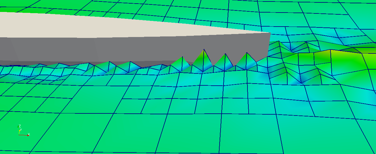
Figure 3: An example of the sawtooth instability developing on the stern of the hull without stabilization.

This approach leads to extremely accurate estimations of the forcing terms in the free-surface evolution equations (39c) and (39d), with a very small computational cost. Unfortunately, the equations right hand sides both contain transport terms (respectively ${\boldsymbol{\nabla}}\eta\cdot\left(\boldsymbol{w}-{\boldsymbol{\nabla}}\phi-\boldsymbol{V}_{\infty}+\boldsymbol{V}_{\text{f}}\right)$ and ${\boldsymbol{\nabla}}\phi\cdot\left(\boldsymbol{w}-{\boldsymbol{\nabla}}\phi-\boldsymbol{V}_{\infty}+\boldsymbol{V}_{\text{f}}\right)$), that become dominant whenever $(\boldsymbol{V}_{\text{f}}-\boldsymbol{V}_{\infty})$ is very different from ${\boldsymbol{\nabla}}\phi$. This causes a sawtooth numerical instability which in most cases develops in proximity of the hull stern, with consequent blow up of the simulations (an example of such instability is given in Figure 3).

A natural, inexpensive and consistent stabilization algorithm which is able toreduce the observed instabilities is the Streamwise Upwind Petrov–Galerkin (SUPG) scheme (see, for example, hughes1979 ; tezduyar2003computation ). The SUPG stabilization consists in replacing the plain $L^{2}$ projection in system (56) with the weighted projection

$$\left(\frac{\delta\phi}{\delta t},\varphi+\boldsymbol{d}\cdot{\boldsymbol{\nabla}}_{s}\varphi\right)_{w}=\left(V_{\phi},\varphi+\boldsymbol{d}\cdot{\boldsymbol{\nabla}}_{s}\varphi\right)_{w}\qquad \forall\varphi\in V_{h}$$ (58a)

$$\left(\frac{\delta\eta}{\delta t},\varphi+\boldsymbol{d}\cdot{\boldsymbol{\nabla}}_{s}\varphi\right)_{w}=\left(V_{\eta},\varphi+\boldsymbol{d}\cdot{\boldsymbol{\nabla}}_{s}\varphi\right)_{w} \forall\varphi\in V_{h},$$ (58b)

where

$$\boldsymbol{d}:=\tau\left(\frac{\boldsymbol{v}-\boldsymbol{w}}{|\boldsymbol{v}-\boldsymbol{w}|}\right).$$ (59)

$\tau$ is a positive stabilization parameter which involves a measure of the local length scale (i.e. the “element length”) and the local Reynolds and Courant numbers. Element lengths and stabilization parameters were proposed for the SUPG formulation of incompressible and compressible flows in hughes1979 , and an in depth study of the stabilization properties for free boundary problems was presented in tezduyar2003computation . However, to the best of the authors’ knowledge, this is the first time that such stabilization technique is applied directly to a boundary value problem defined on a curved surface.

Expressing system 58 in matrix form, we get

$$[M][P_{\Gamma^{w}}]\{\phi\}^{\prime}=[P_{\Gamma^{w}}]\{V_{\phi}\}$$ (60a)

$$[M][P_{\Gamma^{w}}]\{\eta\}^{\prime}=[P_{\Gamma^{w}}]\{V_{\eta}\},$$ (60b)

where the vectors and —sparse— matrices elements are computed by

$$M^{ij}:= \left(\varphi^{j},\varphi^{i}+\boldsymbol{d}\cdot{\boldsymbol{\nabla}}_{s}\varphi^{i}\right)$$

$$= \sum_{k=1}^{M}\int_{\hat{K}}\varphi^{j}_{k}(u,v)\big{(}\varphi^{i}(u,v)+\boldsymbol{d}\cdot{\boldsymbol{\nabla}}_{s}\varphi^{i}(u,v)\big{)}J^{k}(u,v,t)\,\text{d}u\,\text{d}v$$ (61a)

$$P_{A}^{ij}:= \begin{cases}\delta_{ij}&\text{ if }\boldsymbol{x}^{i}(t)\in A(t)\\ 0&\text{ otherwise}\end{cases}$$ (61b)

$$V_{\phi}^{i}:= \left(V_{\phi},\varphi^{i}+\boldsymbol{d}\cdot{\boldsymbol{\nabla}}_{s}\varphi^{i}\right)$$

$$= \sum_{k=1}^{M}\int_{\hat{K}}V_{\phi}(u,v)\big{(}\varphi^{i}(u,v)+\boldsymbol{d}\cdot{\boldsymbol{\nabla}}_{s}\varphi^{i}(u,v)\big{)}J^{k}(u,v,t)\,\text{d}u\,\text{d}v$$ (61c)

$$V_{\eta}^{i}:= \left(V_{\eta},\varphi^{i}+\boldsymbol{d}\cdot{\boldsymbol{\nabla}}_{s}\varphi^{i}\right)$$

$$= \sum_{k=1}^{M}\int_{\hat{K}}V_{\eta}(u,v)\big{(}\varphi^{i}(u,v)+\boldsymbol{d}\cdot{\boldsymbol{\nabla}}_{s}\varphi^{i}(u,v)\big{)}J^{k}(u,v,t)\,\text{d}u\,\text{d}v.$$ (61d)

3.3 Semi-discrete smoothing operator

The semi-discrete version of the smoothing problem (37) can be obtained with a finite element implementation of the scalar Laplace-Beltrami operator, and its application to the different components of $\tilde{\boldsymbol{p}}$.

The weak form of the Laplace-Beltrami operator on $\tilde{\Gamma}$ of a scalar function $u$ in $V$ with Dirichlet boundary conditions $u_{g}$ on $\tilde{\gamma}$ and forcing term $f$ reads

$$\left(\tilde{\boldsymbol{\nabla}}_{s}u,\tilde{\boldsymbol{\nabla}}_{s}\varphi\right)_{\tilde{\Gamma}}=\left(f,\varphi\right)_{\tilde{\Gamma}}\qquad \forall\varphi\in V_{0}$$ (62)

$$u=u_{g}\qquad \text{ on }\tilde{\gamma}.$$

Here, $V_{0}$ denotes the space of functions $\varphi$ in $V$ such that their trace on $\tilde{\gamma}$ is zero (see, for example, BonitoNochettoPauletti-2010-a and the references therein for some details on the numerical implementation of the Laplace-Beltrami operator).

The semi-discrete form of Equation (62) can be written as

$$[K]\{u\}=\{F\},$$ (63)

where

$$K^{ij}:= \left(\tilde{\boldsymbol{\nabla}}_{s}\varphi_{h}^{j},\tilde{\boldsymbol{\nabla}}_{s}\varphi_{h}^{i}\right)$$ (64)

$$= \sum_{k=1}^{M}\int_{\hat{K}}\tilde{\boldsymbol{\nabla}}_{s}\varphi_{k}^{j}(u,v)\cdot\tilde{\boldsymbol{\nabla}}_{s}\varphi_{k}^{i}(u,v)\tilde{J}_{k}(u,v)\,\text{d}u\,\text{d}v$$

$$F^{i}:= \left(f,\varphi_{h}^{i}\right)$$

$$= \sum_{k=1}^{M}\int_{\hat{K}}f_{k}^{j}(u,v)\varphi_{k}^{i}(u,v)\tilde{J}_{k}(u,v)\,\text{d}u\,\text{d}v.$$

The discrete Laplace-Beltrami operator is solved for the auxiliary vector variable $\tilde{\boldsymbol{g}}$, whose finite dimensional representation is given by $\{\boldsymbol{g}\}$. The forcing terms in the system are given by the mean curvature along the normal of $\tilde{\Gamma}$. In this case we write

$$[\boldsymbol{K}]\{\boldsymbol{g}\}=\{\boldsymbol{k}\},$$ (65)

where

$$\begin{split}[\boldsymbol{K}]&:=\begin{bmatrix}[K]&0&0\\ 0&[K]&0\\ 0&0&[K]\end{bmatrix}\\ \{\boldsymbol{k}\}&:=-2k\begin{Bmatrix}\boldsymbol{n}_{x}\\ \boldsymbol{n}_{y}\\ \boldsymbol{n}_{z}\end{Bmatrix}.\end{split}$$ (66)

and the full matrix form of Problem (38) finally reads

$$\left[\alpha\right]\left\{\phi\right\}+\left[N\right]\left\{\phi\right\}-\left[D\right]\left\{\phi_{n}{}\right\} =0$$ (67a)

$$[M][P_{\Gamma^{w}}]\{\phi\}^{\prime}-[P_{\Gamma^{w}}]\{V_{\phi}\} =0$$ (67b)

$$[M][P_{\Gamma^{w}}]\{\eta\}^{\prime}-[P_{\Gamma^{w}}]\{V_{\eta}\} =0$$ (67c)

$$[P_{\Gamma^{w}}]\{\phi(0)\}-[P_{\Gamma^{w}}]\{\phi_{0}\} =0$$ (67d)

$$[P_{\Gamma^{w}}]\{\eta(0)\}-[P_{\Gamma^{w}}]\{\eta_{0}\} =0$$ (67e)

$$[I-P_{\Gamma^{w}}]\{\phi_{n}{}\}-[I-P_{\Gamma^{w}}]\overline{\{\phi_{n}{}\}} =0$$ (67f)

$$[P_{\gamma}]\{\boldsymbol{g}\}^{\prime}-[P_{\gamma}]\{\boldsymbol{w}_{g}\} =0$$ (67g)

$$[\boldsymbol{K}]\{\boldsymbol{g}\}-\{\boldsymbol{k}\} =0$$ (67h)

$$[\mathcal{P}]\{\boldsymbol{g}\}-\{\boldsymbol{x}\} =0,$$ (67i)

where $\mathcal{P}$ is a numerical implementation of the projection operator (39g). On the hull surface, this operator is easily implemented analytically for simple hull shapes, such as that of the Wigley hull. In a more general case, it is desirable to have an implementation of the projection operator which can directly interrogate the CAD files describing the hull surface. In this work, we present results obtained with the former projection. A CAD based projection, which makes use of the OpenCASCADE library opencascade , is currently being implemented. Some work is still required though, to render our full discretization robust with respect to arbitrary hull geometries.

3.4 Time discretization

System (67) can be recast in the following form

$$F(t,y,y^{\prime})=0,$$ (68)

where we grouped the variables of the system in the vector $y$:

$$y=\left\{\begin{array}[]{c}\left\{\boldsymbol{x}\right\}\\ \left\{\phi\right\}\\ \left\{\phi_{n}{}\right\}\end{array}\right\}.$$ (69)

Equation (68) represents a system of nonlinear differential algebraic equations (DAE), which we solve using the IDA package of the SUNDIALS OpenSource library sundials2005 . As stated in the package documentation (see p. 374 and 375 in sundials2005 ):

The integration method in IDA is variable-order, variable-coefficient BDF [backward difference formula], in fixed-leading-coefficient form. The method order ranges from 1 to 5, with the BDF of order $q$ given by the multistep formula

$$\sum_{i=0}^{q}\alpha_{n,i}y_{n-i}=h_{n}\dot{y}_{n},$$ (70)

where $y_{n}$ and $\dot{y}_{n}$ are the computed approximations to $y(t_{n})$ and $y^{\prime}(t_{n})$, respectively, and the step size is $h_{n}=t_{n}-t_{n-1}$. The coefficients $\alpha_{n,i}$ are uniquely determined by the order $q$, and the history of the step sizes. The application of the BDF [in Eq. (70)] to the DAE system [in Eq. (68)] results in a nonlinear algebraic system to be solved at each step:

$$R(y_{n})\equiv F\biggl{(}t_{n},y_{n},h_{n}^{-1}\sum_{i=0}^{q}\alpha_{n,i}y_{n-i}\biggr{)}=0.$$ (71)

Regardless of the method options, the solution of the nonlinear system [in Eq. (71)] is accomplished with some form of Newton iteration. This leads to a linear system for each Newton correction, of the form

$$J[y_{n,m+1}-y_{n,m}]=-R(y_{n,m}),$$ (72)

where $y_{n,m}$ is the $m$th approximation to $y_{m}$. Here $J$ is some approximation to the system Jacobian

$$J=\frac{\partial R}{\partial y}=\frac{\partial F}{\partial y}+\alpha\frac{\partial F}{\partial y^{\prime}},$$ (73)

where $\alpha=\alpha_{n,0}/h_{n}$. The scalar $\alpha$ changes whenever the step size or method order changes.

In our implementation, we assemble the residual $R(y_{n,m})$ at each Newton correction, and let SUNDIALS compute an approximation of the Jacobian in Eq. (73). The final system is solved using a preconditioned GMRES iterative method (see, e.g., GolubVan-Loan-1996-a ).

Despite the increase in computational cost due the implicit solution scheme, the DAE system approach presents several advantages with respect to explicit resolution techniques. First, it is worth pointing out that among the unknowns in equation (69), the coordinates of all the grid nodes (except for the vertical coordinates of free-surface nodes) appear in the DAE system as algebraic components. Their evolution is in fact not described by a differential equation, but computed through the smoothing operator. Yet, the time derivative of such coordinates, i.e.: the ALE velocity $\boldsymbol{w}$ is readily available through the evaluation of the BDF (70). Such velocites are used in the differential Equations (67b) and (67c) which appear in the DAE system. In particular, at each time step, the convergence of Newton corrections (72) ensures that the vertical velocity of the nodes is the one corresponding to the $\boldsymbol{w}$ velocity originated by the horizontal nodes displacement computed by the smoothing operator. In a similar fashion, the DAE solution algorithm computes the ALE time derivative of the velocity potential at each Newton correction. Such derivative is plugged into Bernoulli’s equation (3a) to evaluate the pressure on the whole domain boundary $\Gamma(t)$, without requiring the solution of additional boundary value problems for $\frac{\partial\phi}{\partial t}$. Finally, the resulting pressure field is integrated on the ship wet surface $\Gamma^{h}(t)$ to obtain the pressure force acting on the ship. Since this operation is done at the level of each Newton correction, possible rigid motions of a hull along its six degrees of freedom can be accounted for in a very natural way in the DAE framework, by adding the six differential equations of motion governing the unknown rigid displacements to the DAE system. The latter —strongly coupled— fluid structure interaction model is currently under development and results will be presented in future contributions.

3.5 Adaptive mesh refinement

There are two main advantages of using a Galerkin formulation for the evolution equation of the free-surface, as well as for the computation of the full ALE deformation on the surface $\Gamma(t)$. On one hand, it allows the use of fully unstructured meshes, with an immediate simplification in the mesh generation. On the other hand, it enables the use of a wide set of local refinement strategies based on a posteriori error estimators, which are rather popular in the finite element community. As a result, the mesh generation and adaptation are fully automated, and the resulting computational grids are shaped based on the characteristic of the problem solution, rather than on a-priori heuristic choices.

In this work, we use a modification of the gradient recovery error estimator by Kelly, Gago, Zienkiewicz and Babuska kelly1983posteriori ; gago1983posteriori , a choice mostly motivated by its simplicity (see AinsworthOden-1997-a for more details on this and other error estimators).

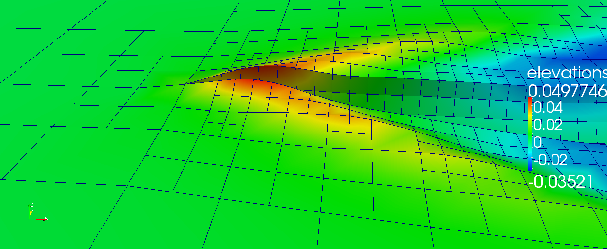
Figure 4: A mesh refinement step.

At fixed intervals in time, the surface gradient of the finite element approximation of $\phi$ is post-processed. This provides a quantitative estimate of the cells in which the approximation error may be higher. In particular, for each cell $K$ of our triangulation we compute the quantity

$$\tau_{K}^{2}:=\frac{h}{24}\int_{\partial K}\left[{\boldsymbol{\nabla}}_{s}\phi\cdot\boldsymbol{n}_{\partial K}\right]^{2}\,\text{d}\gamma,$$ (74)

where $[{\boldsymbol{\nabla}}_{s}\phi\cdot\boldsymbol{n}_{\partial K}]$ denotes the jump of the surface gradient of $\phi$ across the edges of the triangulation element $K$. The vector $\boldsymbol{n}_{\partial K}$ is perpendicular to both the cell normal $\boldsymbol{n}$, and to the boundary of the element $K$, and $h$ is the diamater of the cell itself.

Roughly speaking, $\tau_{K}$ gives an estimate of how well the trial space is approximating the surface gradient of $\phi$. The higher these values are, the smaller the cells should become. The estimated error per cell $\tau_{K}$ is ordered, and a fixed fraction of the cells with the highest and lowest error $\tau_{K}$ are flagged for refinement and coarsening. The computational grid is then refined, ensuring that any two neighboring cells differ for at most one refinement level.

Standard interpolation is used to transfer all finite dimensional solutions from one grid to another, and a geometrically consistent mesh modification algorithm is used to collocate the new nodes coordinates as smoothly as possible (see BonitoNochettoPauletti-2010-a for a detailed explanation of this algorithmic strategy). The resulting computational grid is non conformal. At each hanging node, all the finite dimensional fields are constrained to be continuous. This results in a set of algebraic constraints to be applied to all the degrees of freedom associated with the hanging nodes, which are eliminated from the final system of equations via a matrix condensation technique.

Most of these algorithmic strategies are based on the ones which were already implemented in the deal.II finite element library BangerthHartmannKanschat2007 for trial spaces of finite elements defined in two and three dimensions, and were modified to allow their use on arbitrary surfaces embedded in three dimensions. An example of a refinement step is presented in Figure 4.

After each coarsening and refinement step, the system of differential algebraic equations is restarted with the newly interpolated solution as initial condition. A state diagram for the entire solution process is sketched in Figure 5.

Figure 5: State Diagram

4 Numerical simulations and results

The test case presented in this work is the problem of a Wigley hull advancing in calm water at speed $\boldsymbol{V}_{\infty}$ parallel to the longitudinal axis, with fixed sinkage and trim. In naval engineering, the Wigley hull is commonly used as a benchmark for the validation of free-surface flow simulations. This is mainly due to its simple shape, defined by the equation

$$y(x,z)=\frac{B}{2}\left[1-\left(\frac{2x}{L}\right)^{2}\right]\left[1-\left(\frac{z}{T}\right)^{2}\right].$$ (75)

In our simulations the boat length, beam and draft values used are respectively $L=2.5\ \text{m}$, $B=0.25\ \text{m}$, and $T=0.15625\ \text{m}$. A sketch of the resulting hull shape is presented in Fig. 6, which represents a set of vertical sections of the hull.

Figure 6: Vertical sections of the Wigley hull used for the simulations, generated by planes normal to the longitudinal axis of the hull.

In the numerical simulation setup, the boat is started at rest, and the its velocity is increased up to the desired speed $\boldsymbol{V}_{\infty}$ with a linear ramp. The simulation is then carried on until the flow approaches a steady state solution. The presence of the ramp is not needed for the stability and convergence of the solution, which are also obtained imposing an impulsive start of the water past the hull. Still, inducing slower dynamics in the first seconds of the simulations, the linear ramp allows for higher time steps and faster convergence.

To compare the non linear free-surface BEM solutions with the experimental results presented in mccarthy1985 , we considered six different surge velocities $V_{\infty}$, corresponding to the Froude numbers reported in Table 1. For each of these Froude numbers, numerical solutions were obtained using a refined and a coarse mesh, in which the adaptive mesh refinement algorithm was tuned in order to maintain the cell dimensions over a given minimum value, and in order to limit the number of degrees of freedom under a maximum value.

Despite the fact that the BEM solver developed allows for the use of panels with arbitrary order, the results we present only refer to iso-parametric bilinear elements. The proposed stabilization mechanism seems insufficient for higher order quadrilateral elements, especially when high Froude numbers are considered.

We are currently investigating alternative stabilization procedures as well as finer tuning of the SUPG parameters to increase the robustness of the algorithm when high order panels are used.

$V_{\infty}$	1.2381$\ \frac{m}{s}$	1.3223$\ \frac{m}{s}$	1.4312$\ \frac{m}{s}$	1.5649$\ \frac{m}{s}$	1.7531$\ \frac{m}{s}$	2.0205$\ \frac{m}{s}$
Fr	0.250	0.267	0.289	0.316	0.354	0.408

Table 1: Wigley hull surge velocities imposed in each numerical simulation, and the corresponding Froude numbers $\text{Fr}=\frac{V_{\infty}}{\sqrt{gL}}$.

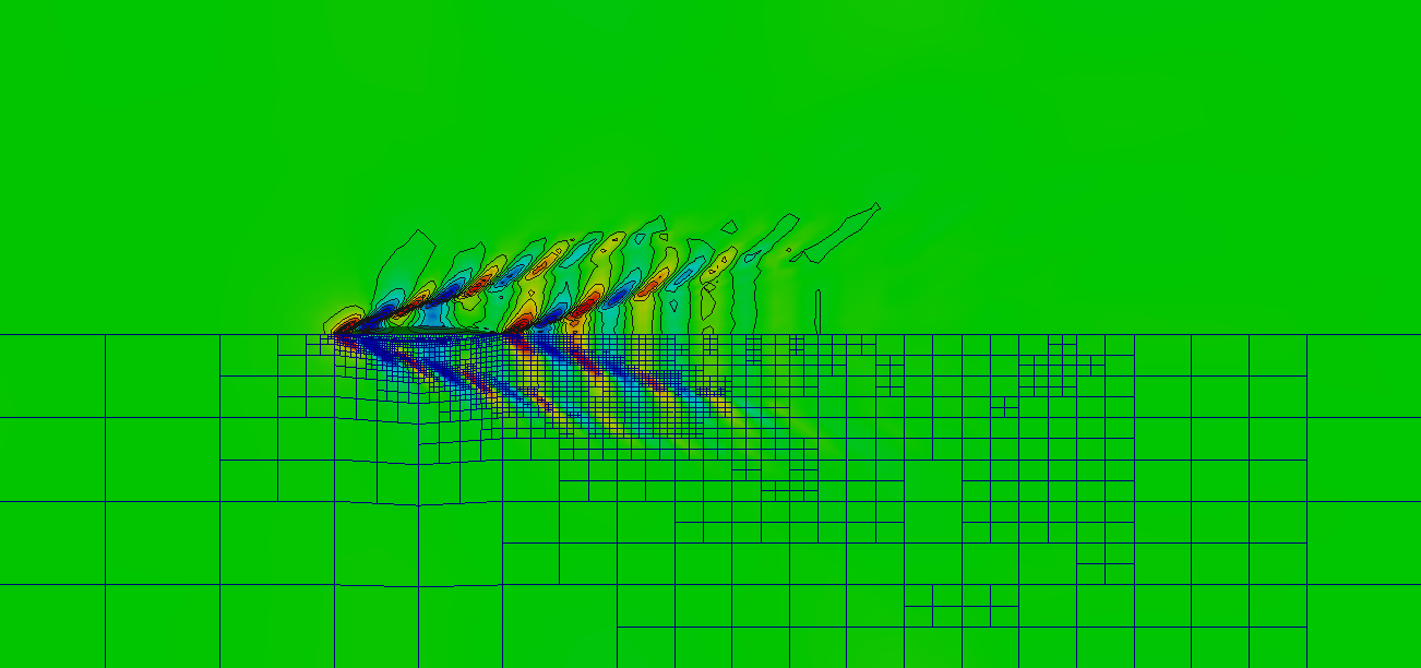
(a) Fr = 0.250

(b) Fr = 0.267

Figure 7: Mesh refinements and contours (I).

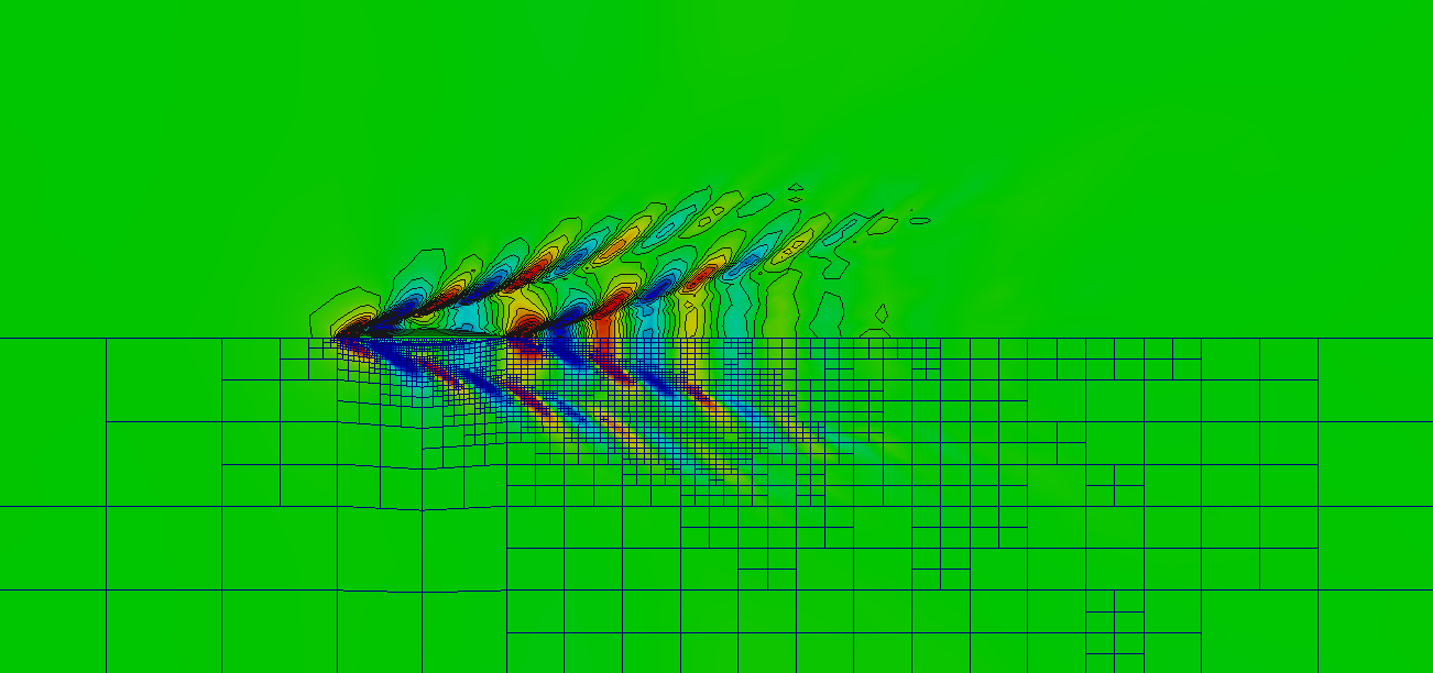
(a) Fr = 0.289

(b) Fr = 0.316

Figure 8: Mesh refinements and contours (II).

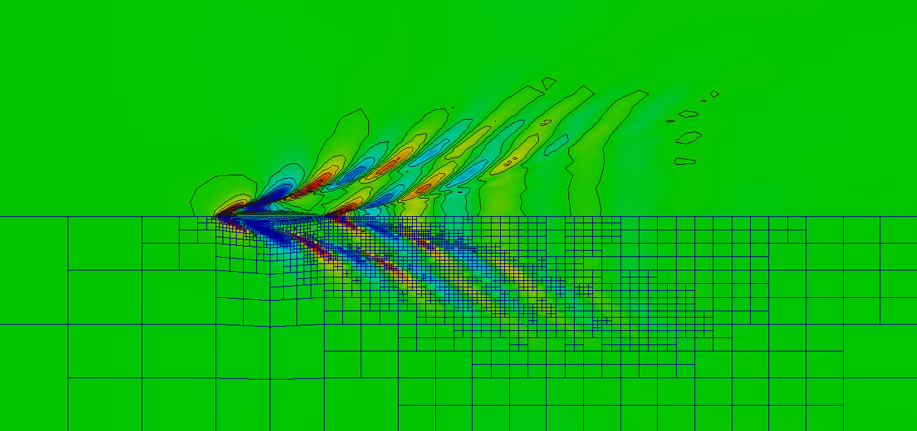
(a) Fr = 0.354

(b) Fr = 0.408

Figure 9: Mesh refinements and contours (III).

A contour of the wave elevation field for the regime solution obtained at the various Froude numbers is presented, along with the final mesh, in Figures 7, 8 and 9. The pictures show how the adaptive mesh refinement leads to an automatic clustering of mesh cells in regions with highest solution gradients. In this way the numerical solutions capture in a very accurate manner the physical characteristics of the wave patterns, requiring a very limited number of degrees of freedom. The biggest final mesh is in fact only composed by roughly 6000 nodes, but it allows for a very good reconstruction of the Kelvin wake, extending for several wavelengths past the surging hull.

The simulations required 12 hrs (for the coarse meshes) to 48 hrs (for the refined meshes) to reach the steady state solution, on single SMP nodes of the Arctur cluster of the Italian/Slovenian interstate cooperation Exact-Lab/Arctur.

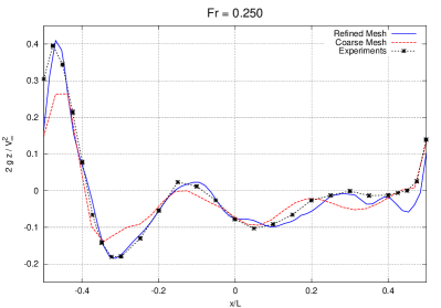
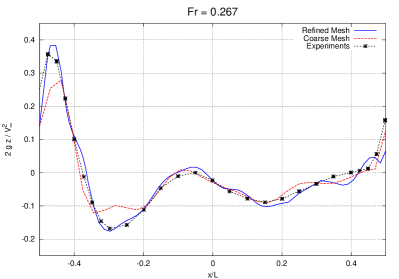
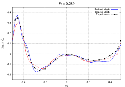
Figure 10: Comparison of predicted water profiles with the University of Tokyo experimental results (- -$\ast$- -). Both coarse mesh (– –) and refined mesh results (—) are shown in the plots.

The wave profiles on the surface of the Wigley hull obtained with the present method, are compared with the corresponding experimental results in Fig. 10. In each plot, the abscissae represent the dimensionless coordinate $x/L$ along the boat, while the ordinates are the dimensionless wave elevations $\eta^{\prime}=\frac{2g\eta}{{V_{\infty}}^{2}}$. For all the Froude numbers considered, the method presented seems able to predict qualitatively correct wave profiles. Moreover, the wave elevation in proximity of the bow of the boat is reproduced with very good accuracy in all the test cases considered. On the other hand, in all the numerical curves, we observe a small spatial oscillation superimposed to the main wave profile. The wave length of such oscillation seems proportional to the local mesh cells size, while the amplitude is slightly higher for finer meshes. This suggests that better tuning of the SUPG stabilization parameter may be needed for this kind of boundary value problems.

5 Conclusions

An accurate and efficient boundary element method for the simulation of unsteady and fully nonlinear potential waves past surging ships was developed, implemented and tested. Compared to existing algorithms, the method presents several innovative features which try to address some of the most CPU intensive aspects of this kind of computations.

The most innovative idea behind the proposed method is the fact that the equations are studied on a fixed reference domain, which is deformed through an arbitrary Lagrangian Eulerian map that keeps track of the physical shape of the water domain around the ship. Some aspects of this approach resemble the semi-Lagrangian formulation of the potential wave equations, but here they are takled using powerful differential geometry tools, combined with finite element techniques for arbitrary surfaces.

This reformulation in terms of a fixed reference domain presents severe stability issues in presence of a forward ship motion, or in presence of an incident stream velocity. Stabilization is achieved via a weighted SUPG projection, which allows the use of fully unstructured meshes, and guarantees an accurate reconstruction of the velocity fields on the mesh nodes, also when low order finite dimensional spaces are used for the numerical discretization.

To the best of the authors’ knowledge, such formulation has never been successfully used in ship hydrodynamic problems in presence of a non zero stream velocity, due to the free-surface instabilities.

With respect to existing methods, the combination of the semi-Lagrangian approach with the SUPG stabilization eliminates the need for periodic remeshing of the computational domain, and opens up the possibility to exploit local adaptivity tools, typical of finite element discretizations.

We exploit these ideas by employing simple a-posteriori error estimates to refine adaptively the computational mesh. Accurate results are obtained even when using a very limited number of degrees of freedom.

Implicit BDF methods with variable order and variable step size are also employed, which render the final computational tool very attractive in terms of robustness.

A direct interface with standard CAD file formats is currently under development, and our preliminary results indicate that the final tool could be used to study the unsteady interaction between arbitrary hull shapes and nonlinear water waves in a robust and automated way.

Appendix A Arbitrary Lagrangian Eulerian Formulation

Figure 11: Schematic representation of a Lagrangian motion and of an arbitrary Lagrangian Eulerian motion.

A motion is a time parametrized family of invertible maps which associates to each point $\hat{\boldsymbol{x}}$ in a reference domain $\hat{\Omega}$ its position in space at time $t$:

$$\hat{\boldsymbol{p}}:\hat{\Omega}\times\mathbb{R}\mapsto\mathbb{R}^{3},\qquad(\hat{\boldsymbol{x}},t)\mapsto\boldsymbol{x}=\hat{\boldsymbol{p}}(\hat{\boldsymbol{x}},t).$$ (76)

The domain $\Omega(t)$ at the current time can be seen as the image under the motion $\hat{\boldsymbol{p}}$ of a reference domain $\hat{\Omega}$, i.e., $\hat{\boldsymbol{p}}(\hat{\Omega},t)=\Omega(t)$. We will indicate with the $\hat{\cdot}$ symbol a material motion, or a motion in which the points $\hat{\boldsymbol{x}}$ label material particles.

If one does not want to follow material particles with the domain $\Omega(t)$, it is possible to introduce another intermediate motion, called the ALE motion, with which we represent deformations of the domain $\Omega(t)$:

$$\tilde{\boldsymbol{p}}:\tilde{\Omega}\times\mathbb{R}\mapsto\mathbb{R}^{3},\qquad(\tilde{\boldsymbol{x}},t)\mapsto\boldsymbol{x}=\tilde{\boldsymbol{p}}(\tilde{\boldsymbol{x}},t).$$ (77)

These motions can be rather arbitrary, as long as the shape of the domain $\Omega(t)$ is preserved by the motion itself, i.e., $\tilde{\boldsymbol{p}}(\tilde{\Omega},t)=\Omega(t)$. The points labelled with $\tilde{\boldsymbol{x}}$ do not, in general, represent material particles. See Figure 11 for a schematic representation of a Lagrangian motion and of an ALE motion.

Given a Lagrangian field $\hat{q}:\hat{\Omega}\times\mathbb{R}\mapsto\mathbb{R}$, its Eulerian representation is

$$q(\boldsymbol{x},t):=\hat{q}(\hat{\boldsymbol{p}}^{-1}(\boldsymbol{x},t),t),\qquad\forall\boldsymbol{x}\in\Omega(t),$$ (78)

while, given an Eulerian field $q:\Omega(t)\times\mathbb{R}\mapsto\mathbb{R}$, its Lagrangian representation would be

$$\hat{q}(\hat{\boldsymbol{x}},t):=q(\hat{\boldsymbol{p}}(\hat{\boldsymbol{x}},t),t),\qquad\forall\hat{\boldsymbol{x}}\in\hat{\Omega}.$$ (79)

A similar structure is valid for ALE fields:

$$q(\boldsymbol{x},t) :=\tilde{q}(\tilde{\boldsymbol{p}}^{-1}(\boldsymbol{x},t),t),\qquad \forall\boldsymbol{x}\in\Omega(t),$$ (80)

$$\tilde{q}(\tilde{\boldsymbol{x}},t) :=q(\tilde{\boldsymbol{p}}(\tilde{\boldsymbol{x}},t),t), \forall\tilde{\boldsymbol{x}}\in\tilde{\Omega}.$$ (81)

The fluid particle velocity $\boldsymbol{v}$ which appears in Problem (1) is the Eulerian representation of the particles velocity

$$\boldsymbol{v}(\hat{\boldsymbol{p}}(\hat{\boldsymbol{x}},t),t)=\hat{\boldsymbol{v}}(\hat{\boldsymbol{x}},t):=\frac{\partial\hat{\boldsymbol{p}}(\hat{\boldsymbol{x}},t)}{\partial t}.$$ (82)

In a similar way, we define the Eulerian representation of the domain velocity, or ALE velocity the field $\boldsymbol{w}$ such that

$$\boldsymbol{w}(\tilde{\boldsymbol{p}}(\tilde{\boldsymbol{x}},t),t)=\hat{\boldsymbol{w}}(\tilde{\boldsymbol{x}},t):=\frac{\partial\tilde{\boldsymbol{p}}(\tilde{\boldsymbol{x}},t)}{\partial t}.$$ (83)

Time variations of physical quantities associated with material particles are computed at fixed $\hat{\boldsymbol{x}}$, generating the usual material derivative

$$\frac{Dq(\boldsymbol{x},t)}{Dt}:=\left.\frac{\partial q(\hat{\boldsymbol{p}}(\hat{\boldsymbol{x}},t),t)}{\partial t}\right|_{\hat{\boldsymbol{x}}=\hat{\boldsymbol{p}}^{-1}(\boldsymbol{x},t)}=\frac{\partial q(\boldsymbol{x},t)}{\partial t}+\boldsymbol{v}\cdot{\boldsymbol{\nabla}}q(\boldsymbol{x},t).$$ (84)

In a similar fashion, if we compute quantities at fixed ALE point $\tilde{\boldsymbol{x}}$, we obtain the ALE time derivative, wich we will denote as

$$\frac{\delta q(\boldsymbol{x},t)}{\delta t}:=\left.\frac{\partial q(\tilde{\boldsymbol{p}}(\tilde{\boldsymbol{x}},t),t)}{\partial t}\right|_{\tilde{\boldsymbol{x}}=\tilde{\boldsymbol{p}}^{-1}(\boldsymbol{x},t)}=\frac{\partial q(\boldsymbol{x},t)}{\partial t}+\boldsymbol{w}\cdot{\boldsymbol{\nabla}}q(\boldsymbol{x},t).$$ (85)

The ALE deformation allows one to define the equations of motions in Problem (1) in terms of the fixed ALE reference domain $\tilde{\Omega}$, while still solving the same physical problem. On the free-surface part of the boundary, the ALE motion needs to follow the evolution of the fluid particles in order to maintain the correct shape of the domain $\Omega(t)$, in particular the minimum requirement for the ALE motion on the free-surface is given by the free-surface kinematic boundary condition

$$\boldsymbol{w}\cdot\boldsymbol{n}=\boldsymbol{v}\cdot\boldsymbol{n}\qquad\text{ on }\Gamma^{w}(t),$$ (86)

which complements the dynamic boundary condition (1c), and provides an evolution equation for the normal part of the ALE motion on the boundary $\Gamma^{w}(t)$. In terms of the ALE motion, the above condition reads

$$\frac{\partial\tilde{\boldsymbol{p}}}{\partial t}(\tilde{\boldsymbol{x}},t)\cdot\boldsymbol{n}=\boldsymbol{v}(\tilde{\boldsymbol{p}}(\tilde{\boldsymbol{x}},t),t)\cdot\boldsymbol{n}\qquad\text{ on }\Gamma^{w}(t).$$ (87)

Equations (1c) and (86) are usually referred to as the free-surface dynamic and kinematic boundary conditions, since they represent the physical condition applied to the free-surface (equilibrium of the pressure on the water surface) and its evolution equation (the shape of the free-surface follows the velocity field of the flow).

Appendix B Numerical beach

A draw back of using an homogeneous Neumann boundary conditions for the vertical far field boundary condition is that it reflects energy back in the computational domain.

We use an absorbing beach technique (see, for example, CaoBeckSchultz-1993 ), in which we add an artificial damping region away from the boat, used to absorb the wave energy. A damping term can be seen as an additional pressure $P$ acting on the free surface. In such case, Bernoulli equation on the free-surface becomes

$$\frac{\partial\Phi}{\partial t}+gz-\boldsymbol{a}_{\text{s}}\cdot\boldsymbol{x}+\frac{1}{2}|{\boldsymbol{\nabla}}\Phi|^{2}+\frac{P}{\rho}=0\qquad\qquad\text{ on }\ \ \Gamma^{w}(t),$$ (88)

and one can show that the resulting rate of energy absorption is

$$\frac{dE_{f}}{dt}=\int_{\Gamma^{w}}P\phi_{n}{}\,\text{d}\Gamma.$$ (89)

A natural way to construct the damping pressure $P$ is then to use a term which is proportional to the potential normal derivative $\phi_{n}{}$, which grants a positive energy absorption at all times.

The dynamical free-surface boundary condition modified to account for the damping term reads

$$\frac{\partial\Phi}{\partial t}+gz-\boldsymbol{a}_{\text{s}}\cdot\boldsymbol{x}+\frac{1}{2}|{\boldsymbol{\nabla}}\Phi|^{2}-\mu\phi_{n}{}=0\qquad\qquad\text{ on }\ \ \Gamma^{w}(t),$$ (90)

where

$$\mu=\left(\frac{\max\left(0,x-x_{d}\right)}{L_{d}}\right)^{2},$$ (91)

and $x_{d}$ is the $x$ coordinate value in which the artificial damping starts to act, while $L_{d}$ is the length of the absorbing beach, as in Figure 1.

Appendix C Iso-parametric discretization

We approximate the geometry of the domain boundary by means of arbitrary order quadrilateral panels. The edges of each panel are defined by polynomial functions, while their internal surface is described by polynomial tensor products.

Figure 12: A linear panel and the reference element. The red dots represent the additional degrees of freedom of a quadratic panel.

In particular we employ the Lagrangian shape functions $N_{l}(u,v)\quad l=1,\dots,N_{L}$ on the reference panel (Fig. 12, on the left). Thus, the local parametrization of the $k$-th panel reads

$$\begin{split}\tilde{\boldsymbol{x}}_{k}(u,v)&:=\sum_{l=1}^{N_{L}}\tilde{\boldsymbol{x}}^{k_{l}}N_{l}(u,v)\qquad\qquad u,v\in[0,1]^{2}\\ \boldsymbol{x}_{k}(u,v,t)&:=\sum_{l=1}^{N_{L}}\boldsymbol{x}^{k_{l}}(t)N_{l}(u,v)\qquad\qquad u,v\in[0,1]^{2}.\end{split}$$ (92)

The parametrization weights in Eq. (92) are the positions of the nodes in the reference domain $\tilde{\Gamma}_{h}$, or in the current domain $\Gamma_{h}(t)$. $k_{l}$ denotes the local to global numbering index which identifies the $N_{L}$ basis functions $\varphi^{k_{l}}$ which are different from zero on the $k$-th panel.

The global basis functions $\varphi^{i}(\tilde{\boldsymbol{x}})$ can be identified and evaluated on each panel $K$ via their local parametrization as

$$\varphi^{i}_{k}(u,v):=\varphi^{i}(\tilde{\boldsymbol{x}}_{k}(u,v))=\sum_{l=1}^{N_{L}}\delta_{i\,k_{l}}N_{l}(u,v),\qquad\delta_{ij}=\begin{cases}1&\text{ if }i=j\\ 0&\text{ otherwise.}\end{cases}$$ (93)

In this framework, the local representation of $\phi(\boldsymbol{x}^{k}(u,v,t),t)$ and of its normal derivative on the $k$-th panel are

$$\phi_{k}(u,v,t)=\sum_{l=1}^{N_{L}}\phi^{k_{l}}(t)N_{l}(u,v)\qquad\phi_{n}{}{}_{k}(u,v,t)=\sum_{l=1}^{N}\phi_{n}{}^{k_{l}}(t)N_{l}(u,v),$$ (94)

where $\phi^{k_{l}},\phi_{n}{}^{k_{l}}\,\,l=1,\dots,N_{L}$ are the nodal values of the potential and of its normal derivative in panel $k$. On each point of the panel, it is possible to compute two vectors tangential to $\Gamma_{h}(t)$ as

$$\boldsymbol{t}_{u}^{k}(u,v,t)=\sum_{l=1}^{N_{L}}\boldsymbol{x}^{k_{l}}(t)\frac{\partial N_{l}}{\partial u}(u,v)\qquad\boldsymbol{t}_{v}^{k}(u,v,t)=\sum_{l=1}^{N_{L}}\boldsymbol{x}^{k_{l}}(t)\frac{\partial N_{l}}{\partial v}(u,v),$$ (95)

from which the external normal unit vector $\boldsymbol{n}$ is obtained as

$$\boldsymbol{n}_{vect}^{k}(u,v,t)=\boldsymbol{t}_{u}^{k}(u,v,t)\times\boldsymbol{t}_{v}^{k}(u,v,t),\qquad\boldsymbol{n}^{k}(u,v,t)=\frac{\boldsymbol{n}_{vect}^{k}(u,v,t)}{\left|\boldsymbol{n}_{vect}^{k}(u,v,t)\right|}.$$ (96)

The same can be done for vectors tangential and normal to $\tilde{\Gamma}$, by simply replacing $\boldsymbol{x}^{k_{l}}(t)$ with $\tilde{\boldsymbol{x}}^{k_{l}}$ in the definitions above. We will denote those vectors with $\tilde{\boldsymbol{t}}_{u}^{k}(u,v)$, $\tilde{\boldsymbol{t}}_{v}^{k}(u,v)$, $\tilde{\boldsymbol{n}}_{vect}^{k}(u,v)$ and $\tilde{\boldsymbol{n}}^{k}(u,v)$, respectively.

Integrals on a panel $K$ (or $\tilde{K}$), can be computed in the reference domain $[0,1]^{2}$, by observing that $\,\text{d}\Gamma=J^{k}(u,v,t)\,\text{d}u\,\text{d}v$, where $J^{k}(u,v,t):=|\boldsymbol{n}_{vect}^{k}(u,v,t)|$ (or $\,\text{d}\tilde{\Gamma}=\tilde{J}^{k}(u,v)\,\text{d}u\,\text{d}v$, where $\tilde{J}^{k}(u,v):=|\tilde{\boldsymbol{n}}_{vect}^{k}(u,v)|$).

We finally introduce the following differential operators

$$\begin{split}D_{k}(u,v,t)&:={\boldsymbol{\nabla}}_{uv}\boldsymbol{x}_{k}(u,v,t)\qquad\in\mathbb{R}^{3\times 2}\\ G_{k}(u,v,t)&:=D_{k}(u,v,t)^{T}D_{k}(u,v,t)\qquad\in\mathbb{R}^{2\times 2}\\ \tilde{D}_{k}(u,v)&:={\boldsymbol{\nabla}}_{uv}\tilde{\boldsymbol{x}}_{k}(u,v)\qquad\in\mathbb{R}^{3\times 2}\\ \tilde{G}_{k}(u,v)&:=\tilde{D}_{k}(u,v)^{T}\tilde{D}_{k}(u,v)\qquad\in\mathbb{R}^{2\times 2},\end{split}$$ (97)

where $G_{k}$ and $\tilde{G}_{k}$ are the first fundamental forms in the element $K$ and $\tilde{K}$. Making use of such operators, we can express the local surface gradients of the global basis functions as

$$\begin{split}\left.{\boldsymbol{\nabla}}_{s}\varphi^{i}(\tilde{\boldsymbol{p}}^{-1}(\boldsymbol{x},t))\right.|_{\boldsymbol{x}=\boldsymbol{x}_{k}(u,v,t)}&=D_{k}(G_{k})^{-1}\nabla_{uv}\varphi^{i}_{k}(u,v,t)\\ &=:{\boldsymbol{\nabla}}_{s}\varphi^{i}_{k}(u,v,t)\\ \left.\tilde{\boldsymbol{\nabla}}_{s}\varphi^{i}(\tilde{\boldsymbol{x}})\right.|_{\tilde{\boldsymbol{x}}=\tilde{\boldsymbol{x}}_{k}(u,v)}&=\tilde{D}_{k}(G_{k})^{-1}\nabla_{uv}\varphi^{i}_{k}(u,v)\\ &=:\tilde{\boldsymbol{\nabla}}_{s}\varphi^{i}_{k}(u,v),\end{split}$$ (98)

which we will indicate with the same symbol as the spatial surface gradients. The surface gradient of a finite dimensional vector can then be computed by Equation (48).

Appendix D Nomenclature

Bibliography

Bibliography

- [1] OpenCASCADE Technology. http://www.opencaseade.org.
- [2] M. Ainsworth and J.T. Oden. A posteriori error estimation in finite element analysis. Computer Methods in Applied Mechanics and Engineering, 142(1-2):1–88, 1997.
- [3] W. Bangerth, R. Hartmann, and G. Kanschat. deal.II – a general purpose object oriented finite element library. ACM Transactions on Mathematical Software, 33(4):24/1–24/27, 2007.
- [4] R. F. Beck. Time-domain computations for floating bodies. Applied Ocean Research, 16:267–282, 1994.
- [5] R.F. Beck, Y. Cao, and T.H. Lee. Fully nonlinear water wave computations using the desingularized method. In Proceedings of the 6th International Conference on Numerical Ship Hydrodynamics, University of Iowa, 1993.
- [6] A. Bonito, R. H. Nochetto, and M. S. Pauletti. Geometrically consistent mesh modification. SIAM Journal on Numerical Analysis, 48(5):1877–1899, 2010.
- [7] Y. Cao, R.F. Beck, and W. Schultz. An absorbing beach for numerical simulations of nonlinear waves in a wave tank. In Proceedings of the 8th International Workshop on Water Waves and Floating Bodies, St. John’s, Newfoundland, 1993.
- [8] T.A. Cruse. An improved boundary-integral equation method for three dimensional elastic stress analysis. Computers & Structures, 4(4):741–754, 1974.
- [9] M.C. Delfour and J.P. Zolésio. Shapes and Geometries: Metrics, Analysis, Differential Calculus, and Optimization, volume 22. Society for Industrial Mathematics, 2010.
- [10] L. Formaggia, A. Quarteroni, and A. Veneziani. Cardiovascular Mathematics: Modeling and simulation of the circulatory system, volume 1. Springer Verlag, 2009.
- [11] D.S.R. Gago, DW Kelly, OC Zienkiewicz, and I. Babuska. A posteriori error analysis and adaptive processes in the finite element method: Part II–Adaptive mesh refinement. International journal for numerical methods in engineering, 19(11):1621–1656, 1983.
- [12] Gene H. Golub and Charles F. Van Loan. Matrix computations. Johns Hopkins Studies in the Mathematical Sciences. Johns Hopkins University Press, Baltimore, MD, third edition, 1996.
- [13] S. T. Grilli, P. Guyenne, and F. Dias. A fully non-linear model for three-dimensional overturning waves over an arbitrary bottom. International Journal for Numerical Methods in Fluids, 35:829–867, 2001.
- [14] S. T. Grilli and I. A. Svendsen. Corner problems and global accuracy in the boundary element solution of nonlinear wave flows. Engineering Analysis with Boundary Elements, 7(4):178–195, 1990.
- [15] A. C. Hindmarsh, P. N. Brown, K. E. Grant, S. L. Lee, R. Serban, D. E. Shumaker, and C. S. Woodward. Sundials: Suite of nonlinear and differential/algebraic equation solvers. ACM Transactions on Mathematical Software, 31(3):363–396, 2005.
- [16] T.J.R. Hughes and A. Brooks. A multidimensional upwind scheme with no crosswind diffusion. Finite element methods for convection dominated flows, 34:19–35, 1979.
- [17] DW Kelly, D.S.R. Gago, OC Zienkiewicz, and I. Babuska. A posteriori error analysis and adaptive processes in the finite element method: Part I–error analysis. International Journal for Numerical Methods in Engineering, 19(11):1593–1619, 1983.
- [18] M. Kjellberg, G. Contento, and C.E. Janson. A nested domains technique for a fully-nonlinear unsteady three-dimensional boundary element method for free-surface flows with forward speed. In 21st International Offshore and Polar Engineering Conference, ISOPE-2011; Maui, HI; 19 June 2011 through 24 June 2011, pages 673–679, 2011.
- [19] J.C. Lachat and J.O. Watson. Effective numerical treatment of boundary integral equations: a formulation for three-dimensional elastostatics. International Journal for Numerical Methods in Engineering, 10(5):991–1005, 1976.
- [20] J.H. McCarthy. Collected experimental resistance component and flow data for three surface ship model hulls. Technical Report DTNSRDC-85/011, David W. Taylor Research Center, 1985.
- [21] S. Ryu, M. H. Kim, and P. J. Lynett. Fully nonlinear wave-current interactions and kinematics by a bem-based numerical wave tank. Computational Mechanics, 32:336–346, 2003.
- [22] S. M. Scorpio. Fully nonlinear ship-wave computations using a multipole accelerated, desingularized method. PhD thesis, University of Michigan, 1997.
- [23] H. G Sung and S. T. Grilli. Bem computations of 3d fully nonlinear free surface flows caused by advancing surface disturbances. Journal of Offshore and Polar Engineering, 18:292–301, 2008.
- [24] K. Tanizawa. The state of the art on numerical wave tank. In Proceeding of 4th Osaka Colloquium on Seakeeping Performance of Ships, Osaka, pages 95–114, 2000.
- [25] T.E. Tezduyar. Computation of moving boundaries and interfaces and stabilization parameters. International Journal for Numerical Methods in Fluids, 43(5):555–575, 2003.