$\chi_{QJ}\to\ell^{+}\ell^{-}$ within and beyond the Standard Model

Abstract

We revisit $\chi_{QJ}\to\ell^{+}\ell^{-}$ (with $J=0,1,2$ and $Q=b,c$) within the Standard Model (SM). The electro-magnetic contributions are given in color-singlet model with non-vanishing lepton masses at the leading order of $v$. Numerically, the branching ratios of $\chi_{QJ}\to\ell^{+}\ell^{-}$ predicted within the SM are so small that such decays are barely possible to be detected at future BESIII and SuperB experiments, but may be possible to be observed at the LHC. We investigate $\chi_{b0}\to\ell^{+}\ell^{-}$ in Type-II 2HDM with large $\tan\beta$, and $\chi_{b2}\to\ell^{+}\ell^{-}$ in the Randall-Sundrum model, to see their chance to be observed in future experiments.

1 Introduction

The leptonic decay of quarkonium, especially the S-wave triplet $J/\psi$ or $\Upsilon$, plays a very important role in particle physics, either due to its clean experimental signal which is commonly used to tag $J/\psi$ or $\Upsilon$ in experiments, or due to its simpleness in theoretical calculations which offers an ideal place for precise determinations of the non-perturbative Non-relativistic QCD (NRQCD) matrix elements Bodwin:1994jh . Thus, $H(^{3}S_{1})\to\ell^{+}\ell^{-}$ has been extensively studied in past almost four decades NLO ; Beneke:1997jm ; Czarnecki:1997vz ; Brambilla:2006ph ; Bodwin:2007ga ; Marquard:2009bj .

However, the leptonic decays of C-even quarkonia are of less interests, because they are generally suppressed in the SM by both of the electromagnetic loop and huge mass of $Z$ boson. The leptonic decay of $\eta_{c}$ is investigated by the method of light-cone wave function in Yang:2009kq and NRQCD factorization at leading order of typical quark velocity $v$ in Jia:2009ip . The leptonic decay of the C-even and P-wave quarkonia (i.e. ${}^{3}P_{J}$ quarkonium $\chi_{QJ}$ ($J=0,1,2$)) has been studied with the color singlet model by Kühn et al about three decades ago Kuhn:1979bb .

In this paper, we will revisit $\chi_{QJ}\to\ell^{+}\ell^{-}$ ($J=0,1,2$ and $Q=b,c$) within the SM. We employ the color-singlet model to calculate the decay amplitudes as Kühn et al did in Kuhn:1979bb . We get the decay amplitudes with finite lepton mass $m_{\ell}$, which are relevant for the helicity-suppressed decay $\chi_{Q0}\to\ell^{+}\ell^{-}$, and $\chi_{bJ}$ or higher ${}^{3}P_{J}$ charmonium excitations decays to $\tau^{+}\tau^{-}$. As it should be, our results agree with those obtained in Kuhn:1979bb by setting $m_{\ell}\to 0$. Furthermore, we calculate the electromagnetic loop by utilizing the method of regionsbeneke:Threthold ; Smirnov:expansion . It allows us to relate our results to those calculated in the conventional NRQCD factorization for the $P$-wave quarkonia decays and productions as in Petrelli:1997ge ; Bodwin:2007zf ; Ma:2002eva .

Phenomenologically, as expected, the decay widths of $\chi_{QJ}\to\ell^{+}\ell^{-}$ are highly suppressed in the SM. It is barely possible to measure such decays even in now-days or near-future high-luminosity colliders, such as BESIII and SuperB, but may be possible to be observed at LHC when the LHC reach its long-term integrated luminosity around 3000 fb^-1. Therefore, in an era longing for the new physics (NP), the smallness of the branching ratios of such decays in the SM can be a virtue. Any experimental discovery of excesses of such decays could be an indication of the NP. Moreover, the quantum numbers of $\chi_{QJ}$ make the NP effects in $\chi_{QJ}\to\ell^{+}\ell^{-}$ spin-dependent. We consider two scenarios of extensions of the SM which may enhance $\chi_{b0}\to\ell^{+}\ell^{-}$ and $\chi_{b2}\to\ell^{+}\ell^{-}$: one is Type-II two Higgs doublet model (2HDM) with large $\tan\beta$ arXiv:1106.0034 , another is the Randall-Sundrum (RS) model for warped extra-dimensions randall-sundrum ; randall-wise .

This paper is organized as follows. In Sect.2, we calculate the decay amplitudes for $\chi_{QJ}\to\ell^{+}\ell^{-}$ within the SM, compare our results with those obtained in Kuhn:1979bb , and discuss briefly the breakdown and restoration of the NRQCD factorization for $\chi_{QJ}\to\ell^{+}\ell^{-}$ along the way that Beneke and Vernazza did for $B\to\chi_{cJ}K$ in Beneke:2008pi . In Sect. 3, we calculate the $\chi_{b0}\to\ell^{+}\ell^{-}$ in Type-II 2HDM, and $\chi_{b2}\to\ell^{+}\ell^{-}$ in the RS model. Sect.4 is devoted for the numerical results and some phenomenological discussions. Finally, we summarize our work in Sect. 5.

2 The decay amplitudes for $\chi_{QJ}\to\ell^{+}\ell^{-}$ within the SM

In the SM, the lowest order Feynman diagrams for $\chi_{QJ}\to\ell^{+}\ell^{-}$ are two electro-magnetic (EM) box-diagrams and a tree-level $Z^{0}$-exchange diagram, depicted in Fig.1. Note that only the ${}^{3}P_{1}$ state can decay into a lepton pair via virtual $Z^{0}$ at tree-level, and the tree-level neutral Higgs exchange diagram for $\chi_{Q0}\to\ell^{+}\ell^{-}$ is neglected.

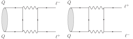
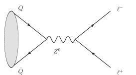
Figure 1: The Feynman diagrams for ${}^{3}P_{J}$ state $Q\bar{Q}$ direct annihilation to lepton pair in the SM. All the Feynman diagrams in this paper are created by JaxoDraw JaxoDraw .

We perform the calculations in the rest frame of quarkonium. The four-momenta of the quark, anti-quark, lepton and anti-lepton are denoted as

$$p_{1} = (E,\textbf{q}\,),~{}~{}p_{2}\,=\,(E,-\textbf{q}\,),$$ (1a)

$$q_{1} = (E,\textbf{q}_{1}\,),~{}~{}q_{2}\,=\,(E,-\textbf{q}_{1}\,).$$ (1b)

where $E=M_{\chi_{QJ}}/2$ with $M_{\chi_{QJ}}$ being mass of $\chi_{QJ}$. We set $2P$ as the total momentum of $Q\bar{Q}$, and $2q$ the relative momentum of $Q\bar{Q}$, i.e.

$$P=\frac{p_{1}+p_{2}}{2}=(E,0)\,,~{}~{}q=\frac{p_{1}-p_{2}}{2}=(0,\textbf{q}).\;$$ (2)

The velocity of the heavy quark is defined as $v\equiv|\textbf{q}|/m_{Q}$.

As in arXiv:0808.1625 ; Sang:2009jc , we describe briefly the procedure to calculate the P-wave quarkonium involved processes within the color singlet model developed by Kühn et al in Kuhn:1979bb .

To project the spin-triplet part of the amplitude
$Q\bar{Q}(^{3}P_{J})\to\ell^{+}\ell^{-}$, we use the covariant projection operator of spin-triplets Bodwin:2002hg

$$\Pi^{\nu}(\text{spin-triplet}) = -\frac{1}{2\sqrt{2}E(E+m_{Q})}(P\hskip-5.89996pt/+q\hskip-4.49997pt/+m_{Q})$$ (3)

$$\times (P\hskip-5.89996pt/+E)\gamma^{\nu}(P\hskip-5.89996pt/-q\hskip-4.49997pt/-m_{Q})\,,$$

to replace the quark-anti-quark spinor bilinear, where $m_{Q}$ is the heavy quark mass. We expand the spin-triplet amplitude as series of the small momentum $q$

$$i\mathcal{M}^{\nu}(q)=i\mathcal{M}^{\nu}(0)+q_{\mu}\frac{\partial}{\partial q_{\mu}}i\mathcal{M}^{\nu}(q)|_{q=0}+\cdots.$$ (4)

Then, the amplitude at the leading order of $v$ for a ${}^{3}P_{J}$ state decay to $\ell^{+}\ell^{-}$ can be obtained through

$$i{\cal M}[^{3}P_{J}\to\ell^{+}\ell^{-}]=|\textbf{q}|\Pi_{\mu\nu}(^{3}P_{J})\frac{\partial}{\partial q_{\mu}}i\mathcal{M}^{\nu}(q)|_{q=0}\,,$$ (5)

with the projectors

$$\Pi_{\mu\nu}(^{3}P_{0})=\frac{1}{\sqrt{3}}\left(-g_{\mu\nu}+\frac{P_{\mu}P_{\nu}}{E^{2}}\right),$$ (6a)

$$\Pi_{\mu\nu}(^{3}P_{1})=\frac{i}{\sqrt{2}E}\epsilon_{\mu\nu\rho\sigma}P^{\rho}\epsilon^{\sigma},$$ (6b)

$$\Pi_{\mu\nu}(^{3}P_{2})=\epsilon_{\mu\nu}\,,$$ (6c)

where $\epsilon_{\sigma}$ and $\epsilon^{\mu\nu}$ are respectively the polarization vector and tensor for the ${}^{3}P_{1}$ and ${}^{3}P_{2}$ states, which satisfy the relations $P^{\mu}\epsilon_{\mu}=0,~{}P^{\mu}\epsilon_{\mu\nu}=0$ and $\epsilon_{\mu}^{~{}\mu}=0$. The polarization summations are Kuhn:1979bb

$$\sum\epsilon_{\mu}\epsilon_{\nu}=-g_{\mu\nu}+\frac{P_{\mu}P_{\nu}}{E^{2}}\equiv\mathbb{P}_{\mu\nu}\,,$$ (7a)

$$\sum\epsilon_{\mu\nu}\epsilon_{\alpha\beta}=\frac{1}{2}\left[\mathbb{P}_{\mu\alpha}\mathbb{P}_{\nu\beta}+\mathbb{P}_{\mu\beta}\mathbb{P}_{\nu\alpha}\right]-\frac{1}{3}\mathbb{P}_{\mu\nu}\mathbb{P}_{\alpha\beta}\,.$$ (7b)

After convoluting the amplitudes in (5) with the radial wave-function for $\chi_{QJ}$ in momentum-space, we reach the final amplitudes for $\chi_{QJ}\to\ell^{+}\ell^{-}$ which is

$$i{\cal M}[\chi_{QJ}\to\ell^{+}\ell^{-}] = -\sqrt{2M_{\chi_{QJ}}N_{c}}\sqrt{\frac{3}{4\pi}}R^{\prime}(0)$$ (8)

$$\times \Pi_{\mu\nu}(^{3}P_{J})\frac{\partial}{\partial q_{\mu}}i\mathcal{M}^{\nu}(q)|_{q=0}\,,$$

where the pre-factor $\sqrt{2M_{\chi_{QJ}}}$ originates from the relativistic normalization of the $\chi_{QJ}$ state, $\sqrt{N_{c}}$ from summation of the colors with $N_{c}=3$ being the number of colors, and $R^{\prime}(0)$ is derivative of the radial wave function of $\chi_{QJ}$ at origin in coordinate-space Kuhn:1979bb .

2.1 Calculation of the box diagrams

We calculate the two box-diagrams depicted in Fig. 1 by use of the method of regions to beneke:Threthold ; Smirnov:expansion . The leading regions in these box diagrams for the ${}^{3}P_{J}$ state decays into lepton pair in expansion of the relative velocity $v$, are: 1) hard region where each component of the momenta of both photons in the loop at order of $m_{Q}$; 2) ultra-soft region where each component of the momentum of one photon at order of $m_{Q}v^{2}$. In each region, the power counting rules of all momenta are clear so that we can perform the $v$-expansion for the loop-integrands straightforwardly. Then we integrate the expanded loop-integrand over the whole momentum space to get the contributions from each region, which sum reproduce the complete amplitudes in a series of $v$.

With all the techniques described above, after some tedious but straightforward calculation, we get the amplitudes from the hard region which are infrared (IR) divergent. Here we use the dimensional regularization (DR) to regulate the IR divergence. The corresponding amplitudes are

$$i\mathcal{M}_{\text{hard}}[^{3}P_{0}\to\ell^{+}\ell^{-}]=-i\frac{2\sqrt{6}\alpha^{2}e^{2}_{Q}}{3\beta m_{Q}^{3}}$$

$$\times\left[\left(\ln\frac{1+\beta}{1-\beta}+\frac{2\beta-\ln\frac{1+\beta}{1-\beta}}{\beta^{2}}\right)\frac{1}{\epsilon_{\text{IR}}}+\text{finite terms}\right]$$

$$\times|\textbf{q}|m_{\ell}\bar{u}(q_{1})v(q_{2})\,,$$ (9a)

$$i\mathcal{M}_{\text{hard}}[^{3}P_{1}\to\ell^{+}\ell^{-}]=-i\frac{2\alpha^{2}e^{2}_{Q}}{\beta m_{Q}^{2}}$$

$$\times\left[\left(\ln\frac{1+\beta}{1-\beta}+\frac{2\beta-\ln\frac{1+\beta}{1-\beta}}{\beta^{2}}\right)\frac{1}{\epsilon_{\text{IR}}}+\text{finite terms}\right]$$

$$\times|\textbf{q}|\bar{u}(q_{1})\gamma_{5}\epsilon\hskip-4.49997pt/v(q_{2})\,,$$ (9b)

$$i\mathcal{M}_{\text{hard}}[^{3}P_{2}\to\ell^{+}\ell^{-}]=i\frac{2\sqrt{2}\alpha^{2}e^{2}_{Q}}{\beta m_{Q}^{3}}$$

$$\times\left[\left(\ln\frac{1+\beta}{1-\beta}+\frac{2\beta-\ln\frac{1+\beta}{1-\beta}}{\beta^{2}}\right)\frac{1}{\epsilon_{\text{IR}}}+\text{finite terms}\right]$$

$$\times|\textbf{q}|\bar{u}(q_{1})\gamma^{\alpha}v(q_{2})q^{1\beta}\epsilon_{\alpha\beta}\,,$$ (9c)

where $\beta\equiv\sqrt{1-m^{2}_{\ell}/m^{2}_{Q}}$ is the velocity of lepton, $\alpha=e^{2}/(4\pi)$ the fine-structure constant, and $e_{Q}$ the electric charge in unit of elementary charge $e$ for the heavy quark $Q$. We do not list the explicit expressions for the finite terms above, since they are somewhat scheme-dependent and therefore meaningless individually. One should notice that $i\mathcal{M}_{\rm hard}[^{3}P_{0}\to\ell^{+}\ell^{-}]$ is proportional to $m_{\ell}$ from the helicity suppression.

In a similar way, we get the contributions from the ultra-soft region to the amplitudes which are ultraviolet (UV) divergent. Here we also use the (DR) to regulate the UV divergence. The corresponding amplitudes are

$$i\mathcal{M}_{\text{us}}[^{3}P_{0}\to\ell^{+}\ell^{-}]=i\frac{2\sqrt{6}\alpha^{2}e^{2}_{Q}}{3\beta m_{Q}^{3}}$$

$$\times\left[\left(\ln\frac{1+\beta}{1-\beta}+\frac{2\beta-\ln\frac{1+\beta}{1-\beta}}{\beta^{2}}\right)\frac{1}{\epsilon_{\text{UV}}}+\text{finite terms}\right]$$

$$\times|\textbf{q}|m_{\ell}\bar{u}(q_{1})v(q_{2})\,,$$ (10a)

$$i\mathcal{M}_{\text{us}}[^{3}P_{1}\to\ell^{+}\ell^{-}]=i\frac{2\alpha^{2}e^{2}_{Q}}{\beta m_{Q}^{2}}$$

$$\times\left[\left(\ln\frac{1+\beta}{1-\beta}+\frac{2\beta-\ln\frac{1+\beta}{1-\beta}}{\beta^{2}}\right)\frac{1}{\epsilon_{\text{UV}}}+\text{finite terms}\right]$$

$$\times|\textbf{q}|\bar{u}(q_{1})\gamma_{5}\epsilon\hskip-4.49997pt/v(q_{2})\,,$$ (10b)

$$i\mathcal{M}_{\text{us}}[^{3}P_{2}\to\ell^{+}\ell^{-}]=-i\frac{2\sqrt{2}\alpha^{2}e^{2}_{Q}}{\beta m_{Q}^{3}}$$

$$\times\left[\left(\ln\frac{1+\beta}{1-\beta}+\frac{2\beta-\ln\frac{1+\beta}{1-\beta}}{\beta^{2}}\right)\frac{1}{\epsilon_{\text{UV}}}+\text{finite terms}\right]$$

$$\times|\textbf{q}|\bar{u}(q_{1})\gamma^{\alpha}v(q_{2})q^{1\beta}\epsilon_{\alpha\beta}\,.$$ (10c)

It is easy to see from (9) and (10), that the divergent parts of hard and ultra-soft parts have opposite signs. Thus, the whole amplitudes for ${}^{3}P_{J}\to\ell^{+}\ell^{-}$ due to the EM interactions

$$i\mathcal{M}_{em}[^{3}P_{J}\to\ell^{+}\ell^{-}] = i\mathcal{M}_{\text{hard}}[^{3}P_{J}\to\ell^{+}\ell^{-}]$$ (11)

$$+ i\mathcal{M}_{\text{us}}[^{3}P_{J}\to\ell^{+}\ell^{-}]$$

are finite.

In all, we have

$$i\mathcal{M}_{em}[\chi_{QJ}\to\ell^{+}\ell^{-}] = -i{\sqrt{2M_{\chi_{QJ}}N_{c}}}\sqrt{\frac{3}{4\pi}}R^{\prime}(0)\frac{e^{2}_{Q}\alpha^{2}}{m_{Q}^{4}}f_{J}$$ (15)

$$\times \left\{\begin{array}[]{ll}m_{\ell}\bar{u}(q_{1})v(q_{2})\,,&J=0\,,\\ m_{Q}\bar{u}(q_{1})\gamma_{5}\epsilon\hskip-4.49997pt/v(q_{2})\,,&J=1\,,\\ \bar{u}(q_{1})\gamma^{\alpha}v(q_{2})q^{1\beta}\epsilon_{\alpha\beta}\,,&J=2\,.\end{array}\right.$$

The finite coefficients $f_{J}(J=0,1,2)$ are from the sums of (9) and (10), their explicit analytic expressions are

$$f_{0} =\frac{2\sqrt{6}\left(2\beta-\left(1-\beta^{2}\right)\ln\left(\frac{\beta+1}{1-\beta}\right)\right)\ln\left(\frac{m_{Q}}{\omega}\right)}{3\beta^{3}}$$

$$+\frac{\sqrt{6}\left(\left(\beta^{2}+2\right)\text{Li}_{2}\left(\frac{\beta-1}{\beta+1}\right)-2\left(\beta^{2}-1\right)\text{Li}_{2}\left(\frac{1-\beta}{\beta+1}\right)\right)}{3\beta^{3}}$$

$$+\frac{1}{2\sqrt{6}\beta^{3}}(4-\beta^{2})\ln^{2}\left(\frac{\beta+1}{1-\beta}\right)$$

$$+\frac{1}{6\sqrt{6}\beta^{3}}\left[\pi^{2}(5\beta^{2}-2)+12\beta\ln(1-\beta^{2})+24\beta\right]$$

$$+\frac{1}{\sqrt{6}\beta^{3}}\ln\left(\frac{\beta+1}{1-\beta}\right)\left[(-2-3i\pi)\beta^{2}-4(1-\beta^{2})\ln(4\beta)\right.$$

$$\left.+2(1-\beta^{2})\ln(1-\beta^{2})+2\right],$$ (17a)

$$f_{1} =\frac{2\left(2\beta-\left(1-\beta^{2}\right)\ln\left(\frac{\beta+1}{1-\beta}\right)\right)}{\beta^{3}}\ln\left(\frac{m_{Q}}{\omega}\right)$$

$$+\frac{\left(1-\beta^{2}\right)}{\beta^{3}}\text{Li}_{2}\left(\left(\frac{1-\beta}{\beta+1}\right)^{2}\right)$$

$$-\frac{2\left(1-\beta^{2}\right)}{\beta^{3}}\left[\left(\ln\left(\frac{4\beta}{\beta+1}\right)-1\right)\ln\left(\frac{\beta+1}{1-\beta}\right)+\frac{\pi^{2}}{12}\right],$$ (17b)

$$f_{2} =\frac{2\sqrt{2}}{\beta^{3}}\left(2\beta-(1-\beta^{2})\ln\left(\frac{\beta+1}{1-\beta}\right)\right)\ln\left(\frac{m_{Q}}{\omega}\right)$$

$$-\frac{\sqrt{2}\left(\beta^{2}-1\right)^{2}\text{Li}_{2}\left(\frac{\beta-1}{\beta+1}\right)}{\beta^{5}}-\frac{2\sqrt{2}\left(\beta^{2}-1\right)\text{Li}_{2}\left(\frac{1-\beta}{\beta+1}\right)}{\beta^{3}}$$

$$-\frac{\left(1-3\beta^{2}\right)\left(1-\beta^{2}\right)\ln^{2}\left(\frac{1-\beta}{\beta+1}\right)}{2\sqrt{2}\beta^{5}}+\frac{1}{\sqrt{2}\beta^{5}}\ln\left(\frac{1-\beta}{\beta+1}\right)$$

$$\times\left[2\beta^{2}(1-\beta^{2})\left(4\ln 2-1-\ln\left(\frac{1-\beta^{2}}{\beta^{2}}\right)\right)\right.$$

$$\left.+(\beta^{4}-1)i\pi+4\beta^{4}\right]+\frac{1}{6\sqrt{2}\beta^{5}}\left[-\pi^{2}(1-\beta^{2})(1+3\beta^{2})\right.$$

$$\left.+4\beta(3+\beta^{2})(2\ln 2-i\pi)\right.$$

$$\left.+16\beta^{3}-12\beta(1+\beta^{2})\ln(1-\beta^{2})\right]\,.$$ (17c)

Here, $\omega=M_{\chi_{QJ}}-2m_{Q}+i\epsilon$ is the binding energy of $\chi_{QJ}$, and $\text{Li}_{2}(x)=-\int_{0}^{x}dt\ln(1-t)/t$ is the dilogarithm function.

In the massless lepton limit $r\equiv m_{\ell}^{2}/m_{Q}^{2}={1-\beta^{2}}\to 0$,

$$f_{0}\to\frac{1}{2\sqrt{6}}\left[16\ln\left(\frac{m_{Q}}{\omega}\right)+3\ln^{2}r+\left(4+6i\pi-12\ln 2\right)\ln r\right.$$

$$\left.~{}~{}~{}~{}~{}~{}+\pi^{2}+8+12\ln^{2}2-12i\pi\ln 2\right],$$ (18a)

$$f_{1}\to 4\ln\frac{m_{Q}}{\omega},$$ (18b)

$$f_{2}\to-\frac{4\sqrt{2}}{3}\left(\ln{2}-3\ln\frac{m_{Q}}{\omega}-1+i\pi\right)\,.$$ (18c)

One can see that $f_{0}$ diverges when $r\to 0$ while $f_{1,2}$ remain finite in the same limit. However, the decay amplitude for $\chi_{Q0}\to\ell^{+}\ell^{-}$ still vanishes when $r\to 0$, since we have singled out the helicity-suppression factor $m_{\ell}$. Finally, we reproduce the results of Kühn et al in Kuhn:1979bb :

$$i\mathcal{M}_{em}[\chi_{Q0} \to\ell^{+}\ell^{-}]\to 0,$$ (19a)

$$i\mathcal{M}_{em}[\chi_{Q1} \to\ell^{+}\ell^{-}]\to-i\sqrt{2M_{\chi_{Q1}}N_{c}}\sqrt{\frac{3}{4\pi}}R^{\prime}(0)$$

$$\times\frac{4e^{2}_{Q}\alpha^{2}}{m^{3}_{Q}}\ln\frac{m_{Q}}{\omega}\bar{u}(q_{1})\gamma_{5}\epsilon\hskip-4.49997pt/v(q_{2}),$$ (19b)

$$i\mathcal{M}_{em}[\chi_{Q2} \to\ell^{+}\ell^{-}]\to-i\sqrt{2M_{\chi_{Q1}}N_{c}}\sqrt{\frac{3}{4\pi}}R^{\prime}(0)$$

$$\times\frac{4\sqrt{2}e^{2}_{Q}\alpha^{2}}{m^{4}_{Q}}\left(\ln\frac{m_{Q}}{\omega}+\frac{1-\ln 2-i\pi}{3}\right)$$

$$\times\epsilon_{\mu\nu}\bar{u}(q_{1})\gamma^{\mu}v(q_{2})\frac{(q_{1}-q_{2})^{\nu}}{2}.$$ (19c)

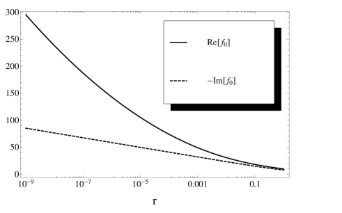
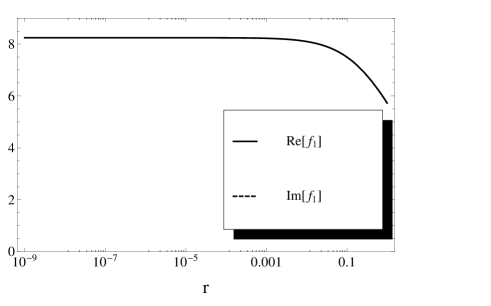
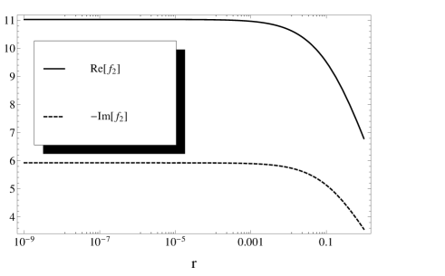
Figure 2: The real and imaginary parts of $f_{i}$ as functions of $r=m_{\ell}^{2}/m_{c}^{2}$.

Taking $\chi_{cJ}$ as examples, we plot the real and imaginary parts of the coefficients $f_{J}$ ($J=0,1,2$) as functions of $r=m_{\ell}^{2}/m_{c}^{2}$ in Fig. 2. We roughly take the $m_{c}=1.65$ GeV and $M_{\chi_{c1,2,3}}=3.41,3.51,3.56$ GeV. $f_{1,2}$ are almost flat when $r\leq 10^{-2}$, but decrease evidently where $r$ is greater than several percent. Thus, our results are useful to make more accurate predictions for $\chi_{bJ}$ or higher radial excitations of $\chi_{cJ}$ decays to $\tau^{+}\tau^{-}$.

Moreover, theoretically, the imaginary parts of $f_{J}$ originate from the on-shell immediate states. In Fig. 2, we see that the imaginary part of $f_{1}$ vanishes because a massive (axial)-vector cannot decay to two photons due to Yang’s theorem c.n.yang . However, one should notice that, if the binding energy $\omega$ can be negative, the $\ln{m_{Q}/\omega}$ term in $f_{1}$ can contribute an imaginary part. And the $\ln\omega$ term comes only from the ultra-soft part in (10). As Kühn et al have pointed out in Kuhn:1979bb , that this effect is related to the E1 transition ${}^{3}P_{J}\to^{3}S_{1}+\gamma$.

2.2 The neutral current contributions

For completeness, we present the neutral current weak interaction contributions to $\chi_{Q1}\to\ell^{+}\ell^{-}$ as follows.

$$i\mathcal{M}_{weak}[\chi_{Q1} \to\ell^{+}\ell^{-}]=\pm iG_{F}\sqrt{\frac{3N_{c}}{\pi M_{\chi_{Q1}}}}R^{\prime}(0)$$

$$\times\bar{u}(q_{1})\epsilon\hskip-4.49997pt/\left(1-4\sin^{2}\theta_{W}-\gamma_{5}\right)v(q_{2})\,,$$ (20)

where the pre-factor “$+$” is for $Q=c$, “$-$” for $Q=b$, $G_{F}$ the Fermi constant, and $\theta_{W}$ the Weinberg angle. As we will see in the numerical analysis, the neutral-current contribution may play an important role, especially in $\chi_{bJ}\to\ell^{+}\ell^{-}$ since its electromagnetic decay amplitude is further suppressed by $e_{b}^{2}=1/9$.

In all, the decay widths for $\chi_{QJ}\to\ell^{+}\ell^{-}$ within the SM can be written as

$$\Gamma[\chi_{Q0}\to\ell^{+}\ell^{-}]=\frac{3N_{c}e^{4}_{Q}\alpha^{4}}{4\pi^{2}m^{4}_{Q}}\beta^{3}(1-\beta^{2})|f_{0}|^{2}|R^{\prime}(0)|^{2}\,,$$ (21)

$$\Gamma[\chi_{Q1}\to\ell^{+}\ell^{-}]=\frac{\beta N_{c}}{8\pi^{2}}|R^{\prime}(0)|^{2}\left[\frac{4e^{4}_{Q}\alpha^{4}}{m^{4}_{Q}}|f_{1}|^{2}\beta^{2}\right.$$

$$\left.+G_{F}^{2}\left(2\beta^{2}g^{2}_{a}+(3-\beta^{2})g^{2}_{v}\right)\pm\frac{4\sqrt{2}e^{2}_{Q}\alpha^{2}G_{F}}{m_{Q}^{2}}\beta^{2}g_{a}\text{Re}[f_{1}]\right]\,,$$ (22)

$$\Gamma[\chi_{Q2}\to\ell^{+}\ell^{-}]=\frac{N_{c}e^{4}_{Q}\alpha^{4}}{20\pi^{2}m^{4}_{Q}}\beta^{3}(5-2\beta^{2})|f_{2}|^{2}|R^{\prime}(0)|^{2}\,,$$ (23)

where $g_{v}={1-4\sin^{2}\theta_{W}}$, $g_{a}=-1$, and “$\pm$” correspond to $Q=c$ and $Q=b$, respectively.

2.3 Connections to the NRQCD factorization

Before we get into phenomenological applications of our results obtained above, we would like to translate our calculations into the language of the effective field theory, and see what we can get from such comparisons.

Heavy quarkonium decays involve three well-separated intrinsic scales $m_{Q},~{}m_{Q}v,~{}m_{Q}v^{2}$. The NRQCD is a suitable and powerful effective field theory to describe the heavy quarkonia production and decays Bodwin:1994jh . By integrating out the hard fluctuations around the scale $m_{Q}$, the effective Lagrangian for the leptonic decay of a non - relativistically moving heavy quark pair $Q\bar{Q}$ can be written as

$$\delta\mathcal{L}= \frac{f(^{3}S_{1})}{m^{2}_{Q}}\mathcal{O}(^{3}S_{1})+\sum\limits_{J=0,1,2}\frac{f(^{3}P_{J})}{m^{4}_{Q}}\mathcal{O}(^{3}P_{J})+\cdots\,,$$ (24)

where $f(^{2S+1}L_{J})$ are the short-distance coefficients supposed to be finite, and the effective operators are

$$\mathcal{O}(^{3}S_{1})=\chi^{\dagger}\gamma^{i}\psi\bar{\ell}\gamma_{i}\ell,$$ (25a)

$$\mathcal{O}(^{3}P_{0})=-\frac{2m_{\ell}}{\sqrt{3}}\chi^{\dagger}\left(-\frac{i}{2}\stackrel{{\scriptstyle\leftrightarrow}}{{D\hskip-5.89996pt/}}\right)\psi\bar{\ell}\ell\,$$ (25b)

$$\mathcal{O}(^{3}P_{1})=-\frac{1}{\sqrt{2}}\chi^{\dagger}\left(-\frac{i}{2}\stackrel{{\scriptstyle\leftrightarrow}}{{D}}\!{}^{i}\left[\gamma_{i},\gamma_{j}\right]\gamma_{5}\right)\psi\bar{\ell}\left[i\not\!\stackrel{{\scriptstyle\leftrightarrow}}{{\partial}},\gamma^{j}\right]\ell,$$ (25c)

$$\mathcal{O}(^{3}P_{2})=\chi^{\dagger}\left[\left(-\frac{i}{2}\right)\stackrel{{\scriptstyle\leftrightarrow}}{{D}}\!{}^{(i}\gamma^{j)}\right]\psi\bar{\ell}\,i\stackrel{{\scriptstyle\leftrightarrow}}{{\partial}}_{(i}\gamma_{j)}\ell.$$ (25d)

Here, following the conventions adopted in Beneke:2008pi , we employ the four-component spinors fields $\psi$ and $\chi$ to represent the the non-relativistic heavy quark and anti-quark, respectively. These fields satisfy $\gamma^{0}\psi=\psi$ and $\gamma^{0}\chi=-\chi$, and are equivalent to the conventional NRQCD two-component fields used in Bodwin:1994jh . The Latin indices $i,j$ run over the spacial indices $1,2,3$, and $(i,j)$ means the traceless part of a symmetric tensor. And

$$\chi^{\dagger}\stackrel{{\scriptstyle\leftrightarrow}}{{D}}\!{}^{i}\Gamma\psi \equiv \chi^{\dagger}D^{i}\Gamma\psi-\chi^{\dagger}\stackrel{{\scriptstyle\leftarrow}}{{D}}\!{}^{i}\Gamma\psi\,,$$ (26)

$$\bar{\ell}\stackrel{{\scriptstyle\leftrightarrow}}{{\partial}}\!{}^{\mu}\Gamma\ell \equiv \bar{\ell}{\partial}\!{}^{\mu}\Gamma\ell-\bar{\ell}\stackrel{{\scriptstyle\leftarrow}}{{\partial}}\!{}^{\mu}\Gamma\ell\,,$$ (27)

where $\Gamma$ denotes any Dirac structure, $D^{i}\equiv\partial^{i}-ig_{s}A^{a,i}T^{a}$ the covariant derivative in QCD. Note that the $P$-wave operators ${\cal O}(^{3}P_{J})$ are $v$-suppressed relative to the $S$-wave operator ${\cal O}(^{3}S_{1})$ due to the power-counting rules in NRQCD.

Neglecting the contributions from weak interaction, at the lowest order of the strong coupling $\alpha_{s}$, we have the expectation $f(^{3}S_{1})$ at $O(\alpha)$ while $f(^{3}P_{J})$ at $O(\alpha^{2})$. Naively, one would expect that

$$i\mathcal{M}[\chi_{QJ}\to\ell^{+}\ell^{-}]=i\frac{f(^{3}P_{J})}{m^{4}_{Q}}\langle\ell^{+}\ell^{-}|\mathcal{O}(^{3}P_{J})|\chi_{QJ}\rangle\,,$$

within the frame of NRQCD at the leading order of $v$. Then, the validation of (2.3) implies a factorization, in which the short-distance contributions are absorbed into $f(^{3}P_{J})$ while all the long-distance contributions are absorbed into the matrix-elements of $\mathcal{O}(^{3}P_{J})$.

However, one should notice that, within the NRQCD, an ultra-soft photon can interact with the heavy quarks, and such interaction can be described by Pineda:1997bj ; Brambilla:1999xf

$$\delta\mathcal{L}_{us} = ee_{Q}\psi^{\dagger}(x)\left[A^{0}_{\text{em}}(t)-\mathbf{x}\cdot\mathbf{E}(t)\right]\psi(x)$$ (29)

$$+ ee_{Q}\chi^{\dagger}(x)\left[A^{0}_{\text{em}}(t)-\mathbf{x}\cdot\mathbf{E}(t)\right]\chi(x)\,,$$

where $A_{\rm em}^{0}$ is the electro-potential, and $\mathbf{E}$ the electro-field strength. Both of $A_{\rm em}^{0}$ and $\mathbf{E}$ have been multipole expanded. In real calculations of the amplitudes, the $A^{0}$ term in (29) can be dropped out either by choosing the temporal gauge $A^{0}_{\rm em}=0$ or by the automatic cancellations in the amplitudes in other gauge choice. The $\mathbf{E}$ term in (29) is actually the electro-dipole interaction, which is at the order $O(v)$ and conserves the spin but change the orbit angular momentum $L$ by one unit. It implies that the ultra-soft photon interaction in (29) can transform a ${}^{3}S_{1}$ state into a ${}^{3}P_{J}$ state with a price of $O(v)$ suppression.

Therefore, the correct decay amplitude for $\chi_{QJ}\to\ell^{+}\ell^{-}$ at the lowest order of $v$ within the NRQCD should be written as

$$i\mathcal{M}[\chi_{QJ}\to\ell^{+}\ell^{-}] = i\frac{f(^{3}P_{J})}{m^{4}_{Q}}\langle\ell^{+}\ell^{-}|\mathcal{O}(^{3}P_{J})|\chi_{QJ}\rangle|_{\text{tree}}$$

$$+ i\frac{f(^{3}S_{1})}{m^{2}_{Q}}\left.\langle\ell^{+}\ell^{-}|\mathcal{O}(^{3}S_{1})|\chi_{QJ}\rangle\right|_{\text{us-loop}}.$$

The matrix-element of $\mathcal{O}(^{3}S_{1})$ above can be depicted by the NRQCD Feynman diagrams in Fig. 3.

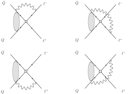
Figure 3: The ultra-soft loop corrections to $\langle\mathcal{O}(^{3}S_{1})\rangle$.

One familiar with the method of regions, can immediately recognize the matching equations

$$i\frac{f(^{3}P_{J})}{m^{4}_{Q}}\langle\ell^{+}\ell^{-}|\mathcal{O}(^{3}P_{J})|\chi_{QJ}\rangle|_{\text{tree}}=i\mathcal{M}_{\rm hard}[\chi_{QJ}\to\ell^{+}\ell^{-}]\,,$$ (31a)

$$i\frac{f(^{3}S_{1})}{m^{2}_{Q}}\left.\langle\ell^{+}\ell^{-}|\mathcal{O}(^{3}S_{1})|\chi_{QJ}\rangle\right|_{\text{us-loop}}=i\mathcal{M}_{\rm us}[\chi_{QJ}\to\ell^{+}\ell^{-}].$$

Consequently, one can find that the “ short-distance” $f(^{3}P_{J})$ does contain IR divergences which breaks down the naive factorization in (2.3).

Of course, the breakdown of the conventional NRQCD factorization for many $P$-wave quarkonium involved processes is not new. Taking $B\to\chi_{cJ}K$ for instance, the QCD factorization breaks down Song:2002mh ; Song:2003yc ; Pham:2005ih ; Meng:2005fc ; Meng:2005er ; Meng:2006mi . However, Beneke and Vernazza showed in Beneke:2008pi , that the factorization for $B\to\chi_{cJ}K$ can be restored, by considering the contribution from $S$-wave color-octet operators in which the chromo-E1 transition analogue to (29) plays a crucial role.

Therefore, the identifications in (31) and finiteness of (2.3) can be regarded as an application of the idea developed by Beneke and Vernazza, to restore the factorization. However, since it deviates from our final phenomenological goal, we would like to stop the further discussions along this line.

3 Possible impacts from new physics beyond the SM

As we have seen, $\chi_{QJ}\to\ell^{+}\ell^{-}$ is highly suppressed in the SM, due to either the EM loop or the large mass of $Z^{0}$. For $\chi_{Q0}\to\ell^{+}\ell^{-}$, it suffers more suppressions in the SM due to the helicity selection rules. The tininess of the branching ratios make such decays sensitive to the possible new physics beyond the SM. If the quantum numbers of the new particles in the SM extensions match those of $\chi_{QJ}$, and the couplings among them are enhanced in some way, we may have a chance to find the hints of new physics in $\chi_{QJ}\to\ell^{+}\ell^{-}$. In this section, we consider two kinds of models: Type-II 2HDM with large $\tan\beta$ arXiv:1106.0034 , and the RS model of the warped extra-dimension randall-sundrum ; randall-wise .

3.1 $\chi_{Q0}\to\ell^{+}\ell^{-}$ in Type-II 2HDM

Type-II 2HDM is one of the most studied extensions of the SM. It shares almost the same Higgs sector interactions with the minimal super-symmetric SM (MSSM). The general Yukawa couplings among the fermions and the lightest neutral Higgs $h$ in 2HDM can be written as

$${\cal L} {}_{Y}^{2HDM}=-\frac{g}{2m_{W}}h$$

$$\times\left(m_{U}\frac{\cos\alpha}{\sin\beta}\bar{U}U-m_{D}\frac{\sin\alpha}{\cos\beta}\bar{D}D-m_{\ell}\frac{\sin\alpha}{\cos\beta}\bar{\ell}\ell\right)\,,$$ (32)

where $U$ denotes for the up-type quarks, $D$ for the down-type quarks, $\ell$ for the charged leptons, $g$ for the SU(2)_L gauge coupling, $\alpha$ for the mixing-angle of the neutral Higgs, and $\tan\beta=v_{u}/v_{d}$ with $v_{d,u}$ being the vacuum expectation values of two Higgs doublets coupled to the down-type and up-type quarks respectively.

Straightforwardly, we have the amplitudes for $\chi_{Q0}\to\ell^{+}\ell^{+}$ via $h$ in Type-II 2HDM are

$$i\mathcal{M}_{2HDM}[\chi_{c0}\to\ell^{+}\ell^{-}] =i4\sqrt{\frac{6N_{c}}{m_{\chi_{c0}}}}G_{F}\frac{\sin 2\alpha~{}m_{c}m_{\ell}}{\sin 2\beta m^{2}_{h}}$$

$$\times\bar{u}(q_{1})v(q_{2})\left(-\sqrt{\frac{3}{4\pi}}R^{\prime}(0)\right)\,,$$ (33)

$$i\mathcal{M}_{2HDM}[\chi_{b0}\to\ell^{+}\ell^{-}] =-i4\sqrt{\frac{6N_{c}}{m_{\chi_{b0}}}}G_{F}\frac{\sin^{2}\alpha~{}m_{b}m_{\ell}}{\cos^{2}\beta m^{2}_{h}}$$

$$\times\bar{u}(q_{1})v(q_{2})\left(-\sqrt{\frac{3}{4\pi}}R^{\prime}(0)\right)\,,$$ (34)

where $m_{h}$ is the mass of the lightest neutral Higgs. Here we have used the relation $4\sqrt{2}G_{F}=g^{2}/m_{W}^{2}$.

In the large $\tan\beta$ scenario of Type II 2HDM, i.e. $\tan\beta\gg 1$ and $\alpha\sim\beta$, the amplitude for $\chi_{b0}\to\ell^{+}\ell^{-}$ is enhanced by the factor $m_{b}m_{\ell}\tan^{2}\beta$, which may compensate the suppression from the factor $m_{h}^{2}$, while $\chi_{c0}\to\ell^{+}\ell^{-}$ does not receive such enhancement. Thus, in the numerical analysis below, we will consider only $\chi_{b0}\to\ell^{+}\ell^{-}$ in Type-II 2HDM with large $\tan\beta$.

3.2 $\chi_{Q2}\to\ell^{+}\ell^{-}$ in the RS model

As a potential solution to the hierarchy problem, the Randall - Sundrum(RS) model randall-sundrum predicts that a TeV Kaluza-Klein (KK) resonances may couple to the SM particles. The corresponding effective Lagrangian is randall-wise

$$\mathcal{L}_{int}=-\frac{\kappa}{m_{0}}h^{KK}_{\mu\nu}T^{\mu\nu}_{SM},$$ (35)

where $h^{KK}_{\mu\nu}$ is the KK graviton field, $T_{SM}$ the SM energy-momentum stress tensor, $\kappa\equiv k/\overline{M}_{Pl}$ the effective coupling constant with $\overline{M}_{Pl}\equiv M_{Pl}/\sqrt{8\pi}$ the reduced Plank scale, $k\sim M_{Pl}$ is the space-time curvature in the extra dimension. $m_{0}=ke^{-k\pi r_{c}}$ is a mass scale at the order of TeV, and the KK graviton masses are $m_{i}=m_{0}x_{i}$, where $r_{c}$ is the compatification radius of the extra dimension, and $x_{i}$ are roots of Bessel function $J_{1}(x)$.

The stress tensor for fermions is proportional to
$\bar{\psi}\left[\left(-\frac{i}{2}\right)\stackrel{{\scriptstyle\leftrightarrow}}{{D}}{}^{(\mu}\gamma^{\nu)}\right]\psi$, which matches to the quantum number of a $2^{++}$ quarkonium. Thus, $\chi_{Q2}\to\ell^{+}\ell^{-}$ can happen at tree-level. Here we consider the contributions from the lowest KK excitations of graviton. A straightforward calculation shows that

$$i\mathcal{M}_{RS}[\chi_{Q2} \to\ell^{+}\ell^{-}]=i2\sqrt{2}\frac{\kappa^{2}}{m^{2}_{1}m^{2}_{0}}\bar{u}(q_{1})\gamma^{\alpha}v(q_{2})$$

$$\times\frac{(q_{1}-q_{2})_{\beta}}{2}\epsilon_{\alpha\beta}\times\left(-\sqrt{\frac{3}{4\pi}}R^{\prime}(0)\right),$$ (36)

and the resulted decay width is

$$\Gamma^{RS}=\frac{32\beta^{3}N_{c}}{5\pi^{2}}|R^{\prime}(0)|^{2}\left(\frac{\kappa}{m_{1}}\right)^{4}\frac{m_{Q}^{4}}{m_{0}^{4}}(5-2\beta^{2}),$$ (37)

where $m_{1}$ is the mass of the lightest KK graviton. Though the KK graviton contribution is TeV scale suppressed, nevertheless, $\chi_{Q2}\to\ell^{+}\ell^{-}$ may be sizable if $\kappa$ is not too small. Since (37) indicates that $\Gamma^{RS}$ is proportional to $m^{4}_{Q}$, we only consider $\chi_{b2}\to\ell^{+}\ell^{-}$ in numerical analysis below.

4 Numerical results and discussions

Here we present the numerical results based on our calculations of $\chi_{QJ}\to\ell^{+}\ell^{-}$ within the SM and beyond. We take the following values for the fine structure constant, Fermi constant and Weinberg angle

$$\alpha=1/137\,,~{}~{}G_{F}=1.16\times 10^{-5}~{}\text{GeV}\,,~{}~{}$$

$$\sin^{2}\theta_{W}=0.231\,,$$ (38)

in our numerical analysis.

4.1 $\chi_{QJ}\to\ell^{+}\ell^{-}$ within the SM

4.1.1 $\chi_{cJ}\to\ell^{+}\ell^{-}$

For $\chi_{cJ}$, we take

$$M(\chi_{c0})=3.41~{}\text{GeV}\,,~{}~{}M(\chi_{c1})=3.51~{}\text{GeV}\,,~{}~{}$$

$$M(\chi_{c2})=3.56~{}\text{GeV}\,,$$ (39)

$$\Gamma(\chi_{c0})=10.3~{}\text{MeV}\,,~{}~{}\Gamma(\chi_{c1})=0.86~{}\text{MeV}\,,~{}~{}$$

$$\Gamma(\chi_{c2})=1.97~{}\text{MeV}\,.$$ (40)

The binding energies are taken as $\omega=M(\chi_{cJ})-2m_{c}$. The derivative of $\chi_{cJ}$ radial wave function at the origin is taken as $|R_{\chi_{c}}^{\prime}(0)|^{2}=0.050$GeV⁵ Beneke:2008pi .

In Table 1, we show the branching ratios of $\chi_{cJ}\to e^{+}e^{-}$ and $\mu^{+}\mu^{-}$ with $m_{c}=1.65$GeV. One can see little difference between the $\text{Br}[\chi_{c1,2}\to e^{+}e^{-}]$ and $\text{Br}[\chi_{c1,2}\to\mu^{+}\mu^{-}]$, but large differences between $\text{Br}[\chi_{c0}\to e^{+}e^{-}]$ and $\text{Br}[\chi_{c0}\to\mu^{+}\mu^{-}]$, because $\chi_{c0}\to\ell^{+}\ell^{-}$ is helicity supressed.

Table 1: The branching ratios of $\chi_{cJ}\to\ell^{+}\ell^{-}$.

Decay Channels	QED	QED+weak
$\chi_{c0}\to e^{+}e^{-}$	$3.19\times 10^{-13}$
$\chi_{c0}\to\mu^{+}\mu^{-}$	$7.06\times 10^{-10}$
$\chi_{c1}\to e^{+}e^{-}$	$4.55\times 10^{-8}$	$3.67\times 10^{-8}$
$\chi_{c1}\to\mu^{+}\mu^{-}$	$4.44\times 10^{-8}$	$3.60\times 10^{-8}$
$\chi_{c2}\to e^{+}e^{-}$	$1.37\times 10^{-8}$
$\chi_{c2}\to\mu^{+}\mu^{-}$	$1.32\times 10^{-8}$

To show the dependence of our results on the charm quark mass, we also plot $\text{Br}[\chi_{cJ}\to e^{+}e^{-}]$ as functions of $m_{c}$ in Fig.4. The curves show the strong dependence of the branching ratios on $m_{c}$, or more precisely the binding energy $\omega$, which is mainly due to the $\ln m_{c}/\omega$ term in the decay amplitudes. And the cusps of the curves also originate from the discontinuity of this logarithmic term.

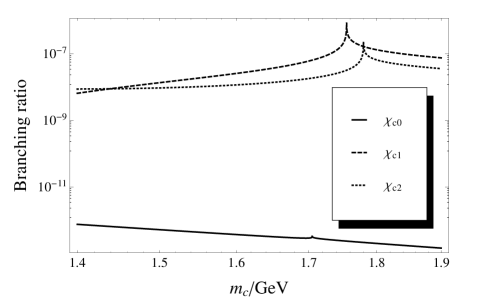
Figure 4: $\text{Br}[\chi_{cJ}\to e^{+}e^{-}]$ as functions of $m_{c}$.

The most of $\chi_{cJ}$ events produced at BEPC-II are from the radiative decays $\psi(2S)\to\chi_{cJ}+\gamma$. BEPC-II will produce about $3.2\times 10^{9}$ $\psi(2S)$ per year. With $\text{Br}[\psi(2S)\to\chi_{c0}+\gamma]=9.62\%$, $\text{Br}[\psi(2S)\to\chi_{c1}+\gamma]=9.2\%$ and $\text{Br}[\psi(2S)\to\chi_{c2}+\gamma]=8.74\%$, we expect that there will be about $2.89\times 10^{8}~{}\chi_{c0}$, $2.76\times 10^{8}~{}\chi_{c1}$ and $2.62\times 10^{8}~{}\chi_{c2}$ produced at BEPC-II annually. From the results listed in Table 1, it seems that there is no possibility to see $\chi_{c0}\to\ell^{+}\ell^{-}$, but marginal possibility to see $\chi_{c1,2}\to\ell^{+}\ell^{-}$ at the BES-III experiments.

4.1.2 $\chi_{bJ}\to\ell^{+}\ell^{-}$

In our calculations, we take the following values for the masses of $\chi_{bJ}$

$$M_{\chi_{b0}}=9.86\,\text{GeV}\,,~{}~{}M_{\chi_{b1}}=9.89\,\text{GeV}\,,$$

$$M_{\chi_{b0}}=9.91\,\text{GeV}\,.$$ (41)

The total decay widths of the $\chi_{bJ}$ are absent in PDG review. $\chi_{bJ}$ decays mainly through annihilations to light hadrons (LH), or radiative radiative transition to $\Upsilon\gamma$ . Although the branching ratios of $\chi_{bJ}\to\Upsilon\gamma$ have been measured experimentally, and the corresponding decay widths can be calculated within certain theoretical models, we will not use those informations to infer the total decay width of $\chi_{bJ}$, since both experimental measurements and theoretical calculations are not so reliable at the present. Instead, we define the ratio between the di-leptonic decay width and light hadronic decay width

$$\mathcal{R}[\chi_{bJ}\to\ell^{+}\ell^{-}]=\frac{\Gamma[\chi_{bJ}\to\ell^{+}\ell^{-}]}{\Gamma[\chi_{bJ}\to\text{LH}]},$$ (42)

to get rough estimates on the orders of magnitudes of the branching ratios of the di-leptonic decays, since the annihilations to light hadrons dominate the decays of $\chi_{bJ}$.

With the decay widths $\Gamma[\chi_{bJ}\to\text{LH}]$ given in Bodwin:1994jh , we have

$$\mathcal{R}[ \chi_{b0}\to\ell^{+}\ell^{-}]=$$

$$\frac{3e^{4}_{b}\alpha^{4}M^{4}_{\chi_{b0}}}{8\pi^{2}\alpha^{2}_{S}m^{4}_{b}}\beta^{3}(1-\beta^{2})\frac{|f_{0}|^{2}}{16+n_{f}M^{2}_{\chi_{bJ}}\rho},$$ (43a)

$$\mathcal{R}[ \chi_{b1}\to\ell^{+}\ell^{-}]=$$

$$\frac{\beta M^{2}_{\chi_{b1}}}{16\pi^{2}\alpha^{2}_{S}n_{f}\rho}\left[\frac{4e^{4}_{b}\alpha^{4}}{m^{4}_{b}}|f_{1}|^{2}\beta^{2}+G_{F}^{2}\left(2\beta^{2}g^{2}_{a}+(3-\beta^{2})g^{2}_{v}\right)\right.$$

$$\left.-\frac{4\sqrt{2}e^{2}_{b}\alpha^{2}G_{F}}{m_{b}^{2}}\beta^{2}g_{a}\text{Re}[f_{1}]\right],$$ (43b)

$$\mathcal{R}[ \chi_{b2}\to\ell^{+}\ell^{-}]=$$

$$\frac{3e^{4}_{b}\alpha^{4}M^{4}_{\chi_{b2}}}{8\pi^{2}\alpha^{2}_{S}m^{4}_{b}}\beta^{3}(5-2\beta^{2})\frac{|f_{2}|^{2}}{64+15n_{f}M^{2}_{\chi_{bJ}}\rho},$$ (43c)

where $n_{f}=4$ is the flavor number of light quarks, $\alpha_{S}$ the strong coupling constant, and $\rho\equiv\frac{\langle\mathcal{O}_{8}(^{1}S_{0})\rangle_{\chi_{bJ}}}{\langle\mathcal{O}_{1}(^{3}P_{J})\rangle_{\chi_{bJ}}}$ which signifies the color-octet contributions to the annihilations to light hadrons. We will use $\rho=0.0021~{}\text{GeV}^{-2}$ as in Bodwin:matrix . Thus, the hadronic uncertainties due to $R^{\prime}(0)$ are greatly reduced in the ratio $\mathcal{R}[\chi_{b0,2}\to\ell^{+}\ell^{-}]$ since $M_{\chi_{b0,2}}^{2}\rho\sim 0.2$. Meanwhile, $\Gamma[\chi_{b1}\to\text{LH}]$ is dominated by the color-octet contribution, so $\mathcal{R}[\chi_{b1}\to\ell^{+}\ell^{-}]$ is still sensitive to parameter $\rho$.

In Table 2, we list $\mathcal{R}[\chi_{bJ}\to\ell^{+}\ell^{-}]$ with $\alpha_{s}(M_{\chi_{bJ}}/2)=0.22$, $m_{b}=4.67$ GeV and $\rho=0.0021~{}\text{GeV}^{-2}$. One can see that the $Z^{0}$-exchange dominates $\chi_{b1}\to\ell^{+}\ell^{-}$, and $\mathcal{R}[\chi_{b1,2}\to\tau^{+}\tau^{-}]$ deviates significantly from $\mathcal{R}[\chi_{b1,2}\to e^{+}e^{-}/\mu^{+}\mu^{-}]$. This makes our recalculations of the EM box diagrams meaningful.

Table 2: The ratio $\mathcal{R}[\chi_{bJ}\to\ell^{+}\ell^{-}]$ with $m_{b}=4.67$ GeV.

Decay Channels	QED	QED+weak
$\chi_{b0}\to e^{+}e^{-}$	$2.31\times 10^{-14}$
$\chi_{b0}\to\mu^{+}\mu^{-}$	$6.80\times 10^{-11}$
$\chi_{b0}\to\tau^{+}\tau^{-}$	$1.51\times 10^{-9}$
$\chi_{b1}\to e^{+}e^{-}$	$3.29\times 10^{-8}$	$6.19\times 10^{-7}$
$\chi_{b1}\to\mu^{+}\mu^{-}$	$3.27\times 10^{-8}$	$6.18\times 10^{-7}$
$\chi_{b1}\to\tau^{+}\tau^{-}$	$2.04\times 10^{-8}$	$4.69\times 10^{-7}$
$\chi_{b2}\to e^{+}e^{-}$	$4.18\times 10^{-9}$
$\chi_{b2}\to\mu^{+}\mu^{-}$	$4.15\times 10^{-9}$
$\chi_{b2}\to\tau^{+}\tau^{-}$	$2.54\times 10^{-9}$

To see the uncertainties of our results due to the bottom quark mass $m_{b}$, we also list the values of $\mathcal{R}[\chi_{bJ}\to\ell^{+}\ell^{-}]$ in Table 3 with several different values of $m_{b}$.

Table 3: $\mathcal{R}[\chi_{bJ}\to\ell^{+}\ell^{-}]$ with different values of $m_{b}$.

$m_{b}$/GeV	4.6	4.8	5.0
$\chi_{b0}\to e^{+}e^{-}$	$2.50\times 10^{-14}$	$2.02\times 10^{-14}$	$1.67\times 10^{-14}$
$\chi_{b0}\to\mu^{+}\mu^{-}$	$7.21\times 10^{-11}$	$6.24\times 10^{-11}$	$6.20\times 10^{-11}$
$\chi_{b0}\to\tau^{+}\tau^{-}$	$1.53\times 10^{-9}$	$1.55\times 10^{-9}$	$2.32\times 10^{-9}$
$\chi_{b1}\to e^{+}e^{-}$	$5.93\times 10^{-7}$	$6.94\times 10^{-7}$	$8.58\times 10^{-7}$
$\chi_{b1}\to\mu^{+}\mu^{-}$	$5.92\times 10^{-7}$	$6.93\times 10^{-7}$	$8.57\times 10^{-7}$
$\chi_{b1}\to\tau^{+}\tau^{-}$	$4.47\times 10^{-7}$	$5.29\times 10^{-7}$	$6.59\times 10^{-7}$
$\chi_{b2}\to e^{+}e^{-}$	$3.71\times 10^{-9}$	$5.76\times 10^{-9}$	$1.84\times 10^{-8}$
$\chi_{b2}\to\mu^{+}\mu^{-}$	$3.68\times 10^{-9}$	$5.73\times 10^{-9}$	$1.83\times 10^{-8}$
$\chi_{b2}\to\tau^{+}\tau^{-}$	$2.21\times 10^{-9}$	$3.63\times 10^{-9}$	$1.23\times 10^{-8}$

According to the estimations in Braguta , the production cross sections of $\chi_{bJ}(J=1,2)$ at LHC ($\sqrt{s}=14$TeV) are

$$\sigma(pp\to\chi_{b0}+X)=1.5\mathrm{\mu b},~{}\sigma(pp\to\chi_{b2}+X)=2\mathrm{\mu b},$$ (44)

so there are about $7.5\times 10^{9}\chi_{b0}$ and $10^{10}\chi_{b2}$ produced in LHC, with present integrated luminosity $5\mathrm{fb}^{-1}$. Thus, there are about 11, 41 and 25 events of $\chi_{b0}\to\tau^{+}\tau^{-}$, $\chi_{b2}\to e^{+}e^{-}(\mu^{+}\mu^{-})$ and $\tau^{+}\tau^{-}$, respectively. Of course, considering the efficiency of the detection, those di-leptonic decays of $\chi_{bJ}$ are not measurable at LHC so far. However, the long-term goal of LHC is to reach a integrated luminosity around $3000\mathrm{fb}^{-1}$ by the end of LHC life. Then, there will be about $6.80\times 10^{3}$ events for $\chi_{b0}\to\tau^{+}\tau^{-}$, $2.51\times 10^{4}$ events for $\chi_{b2}\to e^{+}e^{-}$, $2.49\times 10^{4}$ events for $\chi_{b2}\to\mu^{+}\mu^{-}$, $1.52\times 10^{4}$ events for $\chi_{b2}\to\tau^{+}\tau^{-}$ accumulated at LHC, which make the dileptonic decay of $\chi_{b0,2}$ measurable. So far, there is no estimation on the $\chi_{b1}$ production rate at LHC. Assuming the production rate of $\chi_{bJ}$ is proportional to its decay width to light hadrons, we expect that $\chi_{b1}\to\ell^{+}\ell^{-}$ has a comparable chance to be measured at LHC as $\chi_{b0,2}\to\ell^{+}\ell^{-}$.

4.2 Impacts from new physics

We now consider the numerical impacts on $\chi_{QJ}\to\ell^{+}\ell^{-}$ from the new physics effects. A complete analysis with considering all possible parameters and constrains to parameter space seems rather complicated and deviate from the main topic of the paper. We will perform our analysis by choosing some specific values for the new physics parameters.

4.2.1 $\chi_{b0}\to\ell^{+}\ell^{-}$ in Type-II 2HDM

In general Type-II 2HDM, we have to consider three individual parameters: $m_{h}$, $\tan\beta$ and $\alpha$. Recently, the Higgs mass has been excluded in a broad range of mass parameters. Recently, both the CMS and ATLAS collaborations observed an excess of Higgs-like events with 2-3 sigma around 125 GeV in $pp$ collisions at the Large Hadron Collider (LHC) at $\sqrt{s}=7$ TeV :2012si ; Chatrchyan:2012tx . In the following analysis, we roughly take $m_{h}$ around 125 GeV, although the experimentally observed events may not be referred to the lightest neutral Higgs in 2HDM.

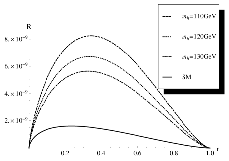
Figure 5: $\mathcal{R}[\chi_{b0}\to\ell^{+}\ell^{-}]$ as functions of $r=m_{\ell}^{2}/m_{b}^{2}$ with $\tan\beta=10$ and different choices of $m_{h}$.

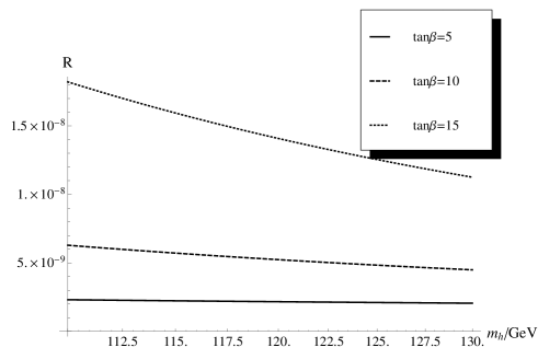
Figure 6: $\mathcal{R}[\chi_{b0}\to\ell^{+}\ell^{-}]$ as functions of $m_{h}$ with different choices of $\tan\beta$.

We first take $\alpha\sim\beta$, while the mass of neutral Higgs $m_{h}$ and $\tan\beta$ are free parameters. We plot $\mathcal{R}[\chi_{b0}\to\ell^{+}\ell^{-}]$ as a function of $r=m^{2}_{\ell}/m^{2}_{b}$ with $\tan\beta=10$ and different values of $m_{h}$, in Fig.5, and also plot $\mathcal{R}$ as a function of $m_{h}$ with $\tan\beta=5\,,10\,,15$ in Fig. 6.

It is easy to see that, when $\tan\beta=10$, the decay width is much larger than the SM results. If $m_{h}$ is taken to be 125GeV, $\mathcal{R}[\chi_{b0}\to\tau^{+}\tau^{-}]$ will be about $4.83\times 10^{-9}$, which is about three times of the SM prediction $1.51\times 10^{-9}$. When $\tan\beta=15$, the dileptonic decay will be enhanced by 8 times. Thus, if Type-II 2HDM is a true theory of our world and $\tan\beta$ is large, we may accumulate more $\chi_{b0}\to\tau^{+}\tau^{-}$ events than the number predicted by SM at LHC.

In general 2HDM, the neutral Higgs mixing angle $\alpha$ is not strongly correlated with $\beta$. To see how $\mathcal{R}[\chi_{b0}\to\ell^{+}\ell^{-}]$ depends on $\alpha$, we plot $\mathcal{R}$ as a function of $\alpha$ with $\tan\beta=5,10$ and $15$, respectively at $m_{h}=125$GeV in Fig.7. $\mathcal{R}[\chi_{b0}\to\tau^{+}\tau^{-}]$ reaches its minimum value $1.51\times 10^{-9}$ when $\alpha=0$ , which is just the SM result, and it reaches its maximum value when $\alpha=\beta$, which is just the case we have discussed above.

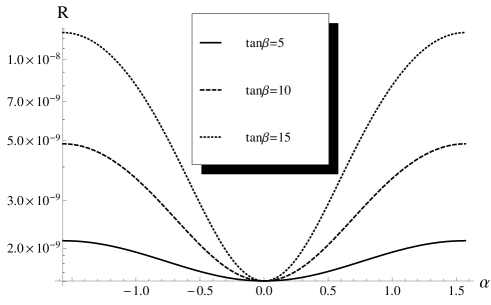
Figure 7: $\mathcal{R}[\chi_{b2}\to\ell^{+}\ell^{-}]$ as functions of $\alpha$ with different choices of $\tan\beta$.

4.2.2 $\chi_{b2}\to\ell^{+}\ell^{-}$ in the RS model

In the RS model, the most important parameters are $\kappa\equiv k/\overline{M}_{Pl}$. Recently, the ATLAS collaboration has reported the 95% C.L. lower limit on the mass of RS graviton for various values of $k/\bar{M_{Pl}}$, which are 0.71,1.03,1.33,1.63TeV for $k/\bar{M_{Pl}}=0.01,0.03,0.05,0.1$, respectively rslimit .

Here, we only consider the decay width induced by the lightest KK excitation of the graviton with neglecting the interference between graviton-exchange and SM contribution. It will not prevent us getting a qualitative observation. We plot the $\mathcal{R}[\chi_{b2}\to\ell^{+}\ell^{-}]$ via the lightest KK graviton as a function of $m_{1}$, with $k/\overline{M}_{Pl}=0.01,0.03,0.05,0.1$ in Fig.8, while the lepton mass $m_{\ell}$ is taken to be 0. From Fig. 8, Table 2 and 3, one can see that, even for $k/\overline{M}_{Pl}\sim 0.1$ and $m_{1}\sim 200$ GeV, the KK graviton exchange cannot compete with the SM contributions in $\chi_{b2}\to\ell^{+}\ell^{-}$. Thus, we have no chance to look for any hints of the RS model in such decay.

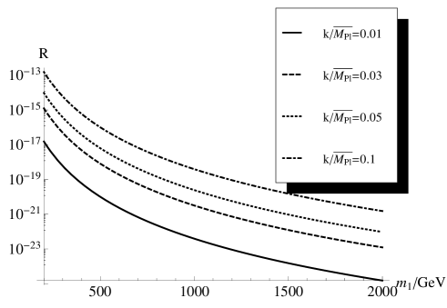
Figure 8: $\mathcal{R}[\chi_{b2}\to\ell^{+}\ell^{-}]$ as function of $m_{1}$ with different choices of $k/\overline{M}_{\rm Pl}$.

5 Summary

In this paper, we recalculate $\chi_{QJ}\to\ell^{+}\ell^{-}$ within the SM by considering the finite mass of the leptons. The suppression of such decays in the SM make them sensitive to the NP. In the future experiments where a huge number of quarkonia are produced, such rare decays of quarkonia could be a new play-ground of NP hunters other than high-energy collisions or flavor changing processes. We investigate $\chi_{b0}\to\ell^{+}\ell^{-}$ in Type-II 2HDM, and $\chi_{b2}\to\ell^{+}\ell^{-}$ in the RS model. We find that in the large $\tan\beta$ limit, we may have better chance to observe $\chi_{b0}\to\tau^{+}\tau^{-}$ in Type-II 2HDM than in the SM, and no chance to find the hints of the RS model in $\chi_{b2}\to\ell^{+}\ell^{-}$. It could be interesting to investigate, in which kind of extensions of the SM, the leptonic decays of $\chi_{QJ}$ might be enhanced so that we can observe them.

Acknowlegement

We thank Yu Jia and Chang-Zheng Yuan for valuable discussions. This work is partly supported by National Natural Science Foundation of China under grant number 10705050 and 10935012.

References

- (1) For reviews of NRQCD, see G. T. Bodwin, E. Braaten, and G. P. Lepage, Phys. Rev. D 51, 1125 (1995); 55, 5853(E) (1997) [arXiv:hep-ph/9407339]; N. Brambilla, A. Pineda, J. Soto and A. Vairo, Rev. Mod. Phys. 77, 1423 (2005) [arXiv:hep-ph/0410047].
- (2) G. T. Bodwin, H. S. Chung, J. Lee and C. Yu, Phys. Rev. D 79, 014007 (2009) [arXiv:0807.2634 [hep-ph]].
- (3) R. Barbieri, R. Gatto, R. Kogerler and Z. Kunszt, Phys. Lett. B 57, 455 (1975).
- (4) M. Beneke, A. Signer and V. A. Smirnov, Phys. Rev. Lett. 80, 2535 (1998) [arXiv:hep-ph/9712302].
- (5) A. Czarnecki and K. Melnikov, Phys. Rev. Lett. 80, 2531 (1998) [hep-ph/9712222].
- (6) N. Brambilla, E. Mereghetti and A. Vairo, JHEP 0608, 039 (2006) [Erratum-ibid. 1104, 058 (2011) ] [arXiv:hep-ph/0604190].
- (7) G. T. Bodwin, J. Lee and C. Yu, Phys. Rev. D 77, 094018 (2008) [arXiv:0710.0995 [hep-ph]].
- (8) P. Marquard, J. H. Piclum, D. Seidel and M. Steinhauser, Phys. Lett. B 678, 269 (2009) [arXiv:0904.0920 [hep-ph]].
- (9) M. Z. Yang, Phys. Rev. D 79, 074026 (2009) [arXiv:0902.1295 [hep-ph]].
- (10) Y. Jia and W. L. Sang, JHEP 0910, 090 (2009) [arXiv:0906.4782 [hep-ph]].
- (11) J. H. Kühn, J. Kaplan and E. G. O. Safiani, Nucl. Phys. B 157, 125 (1979).
- (12) M. Beneke and V. A. Smirnov, Nucl. Phys. B 522, 321 (1998) [hep-ph/9711391].
- (13) V. A. Smirnov, Applied asymptotic expansions in momenta and masses, Springer Tracts Mod. Phys. 177 (Springer, Berlin, 2002).
- (14) A. Petrelli, M. Cacciari, M. Greco, F. Maltoni and M. L. Mangano, Nucl. Phys. B 514, 245 (1998) [arXiv:hep-ph/9707223].
- (15) G. T. Bodwin, E. Braaten, D. Kang and J. Lee, Phys. Rev. D 76, 054001 (2007) [arXiv:0704.2599 [hep-ph]].
- (16) J. P. Ma and Q. Wang, Phys. Lett. B 537, 233 (2002) [arXiv:hep-ph/0203082].
- (17) For a recent review, see G. C. Branco, P. M. Ferreira, L. Lavoura, M. N. Rebelo, M. Sher and J. P. Silva, arXiv:1106.0034 [hep-ph] and references therein.
- (18) L. Randall and R. Sundrum, Phys. Rev. Lett. 83, 3370 (1999) [hep-ph/9905221].
- (19) L. Randall and M. B. Wise, arXiv:0807.1746 [hep-ph].
- (20) M. Beneke and L. Vernazza, Nucl. Phys. B 811, 155 (2009) [arXiv:0810.3575 [hep-ph]].
- (21) D. Binosi and L. Theussl, Comput. Phys. Commun. 161, 76 (2004) [hep-ph/0309015].
- (22) J. Zhang, H. Dong and F. Feng, Phys. Rev. D 84, 094031 (2011) [arXiv:1108.0890 [hep-ph]].
- (23) G. T. Bodwin, E. Braaten, D. Kang and J. Lee, Phys. Rev. D 76, 054001 (2007) [arXiv:0704.2599 [hep-ph]].
- (24) V. V. Braguta, A. K. Likhoded and A. V. Luchinsky, Phys. Rev. D 72, 094018 (2005) [hep-ph/0506009].
- (25) H. S. Chung, J. Lee and C. Yu, Phys. Rev. D 78, 074022 (2008) [arXiv:0808.1625 [hep-ph]].
- (26) W. L. Sang and Y. Q. Chen, Phys. Rev. D 81, 034028 (2010) [arXiv:0910.4071 [hep-ph]].
- (27) G. T. Bodwin and A. Petrelli, Phys. Rev. D 66, 094011 (2002) [arXiv:hep-ph/0205210].
- (28) C. -N. Yang, Phys. Rev. 77, 242 (1950).
- (29) A. Pineda and J. Soto, Nucl. Phys. Proc. Suppl. 64, 428 (1998) [arXiv:hep-ph/9707481].
- (30) N. Brambilla, A. Pineda, J. Soto and A. Vairo, Nucl. Phys. B 566, 275 (2000) [arXiv:hep-ph/9907240].
- (31) Z. -z. Song and K. -T. Chao, Phys. Lett. B 568, 127 (2003) [hep-ph/0206253].
- (32) Z. -Z. Song, C. Meng, Y. -J. Gao and K. -T. Chao, Phys. Rev. D 69, 054009 (2004) [hep-ph/0309105].
- (33) T. N. Pham and G. -h. Zhu, Phys. Lett. B 619, 313 (2005) [hep-ph/0412428].
- (34) C. Meng, Y. -J. Gao and K. -T. Chao, Commun. Theor. Phys. 48, 885 (2007) [hep-ph/0502240].
- (35) C. Meng, Y. -J. Gao and K. -T. Chao, hep-ph/0506222.
- (36) C. Meng, Y. -J. Gao and K. -T. Chao, hep-ph/0607221.
- (37) [ATLAS Collaboration], arXiv:1202.1408 [hep-ex].
- (38) S. Chatrchyan et al. [CMS Collaboration], arXiv:1202.1488 [hep-ex].
- (39) G. Aad, B. Abbott, J. Abdallah, A. A. Abdelalim, A. Abdesselam, O. Abdinov, B. Abi and M. Abolins et al., arXiv:1108.1582 [hep-ex].