Decoherence effect on the Fano lineshapes in double quantum dots
coupled between normal and superconducting leads

Abstract

We investigate the Fano-type spectroscopic lineshapes of the T-shape double quantum dot coupled between the conducting and superconducting electrodes and analyze their stability on a decoherence. Because of the proximity effect the quantum interference patterns appear simultaneously at $\pm\varepsilon_{2}$, where $\varepsilon_{2}$ is an energy of the side-attached quantum dot. We find that decoherence gradually suppresses both such interferometric structures. We also show that at low temperatures another tiny Fano-type structure can be induced upon forming the Kondo state on the side-coupled quantum dot due to its coupling to the floating lead.

I Introduction

When nanoscopic objects such as the quantum dots, nonowires or thin metallic layers are placed in a neighborhood of superconducting material they partly absorb its order parameter. On a microscopic level this proximity effect causes that electrons near the Fermi energy become bound into pairs. Upon forming a circuit with external leads (which can be chosen as conducting, ferromagnetic or superconducting) such effect can induce a number of unique properties in the normal and anomalous tunneling channels Rodero-11 . For instance, the relation between correlations and the on-dot induced pairing has been recently experimentally probed by the Andreev spectroscopy Deacon_etal ; Pillet-10 and the Josephson current measurements Maurand-12 ; Novotny-06 ; Dam-06 ; Cleuziou-06 signifying important role of the Kondo effect on the subgap current.

We address here the Andreev-type transport through the double quantum dot (DQD) nanostructure coupled between the normal (N) and superconducting (S) leads. We focus on the subgap regime, i.e. energies considerably smaller than the pairing gap $\Delta$ of superconductor. Under such conditions eigenstates of the uncorrelated quantum dots are represented either by the singly occupied states $\left|\uparrow\right>$, $\left|\downarrow\right>$ or by coherent superpositions of the empty and doubly occupied configurations $u\left|0\right>+v\left|\uparrow\downarrow\right>$. The resulting Bogolubov-type quasiparticle excitations have an influence on additional spectroscopic features originating for instance from the internal structure, the correlations, perturbations etc. Due to the proximity effect all these appearing structures would show up simultaneously at negative and at positive energies.

To highlight this sort of emerging physics we shall explore in more detail the interference patterns originating from a charge leakage $t$ (assumed to be much weaker than $\Gamma_{N}$ and $\Gamma_{S}$) between the central quantum dot (QD₁) and another side-attached one (QD₂). We also analyze stability of these patterns with respect to a decoherence induced by coupling $\Gamma_{D}$ to the floating lead (D) as sketched in figure 1. Practically this D electrode can mean a substrate on which the quantum dots are deposited or it mimics the effects caused by phonons/photons Gao-08 .

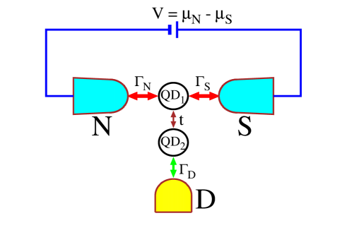
Figure 1: (color online) Schematic view of the T-shape double quantum dot coupled to normal (N) and superconducting (S) electrodes and in addition affected by the floating (D) lead that provides a decoherence.

Without a decoherence the T-shape double quantum dot systems have been already studied theoretically considering both metallic leads (see e.g. Zitko-10 ) and metallic/superconducting ones Tanaka-08 ; Yamada-10 ; Baranski-11 . In the regime of weak interdot coupling $t$ this configuration of the quantum dots enables realization of the Fano-type lineshapes (for a survey on the Fano effect and its realizations in various systems see Ref. Miroshnichenko-10 ). These features can arise when the electron waves transmitted between the external electrodes via a broad QD₁ spectrum happen to interfere with the other electron waves resonantly scattered by the discrete QD₂ levels Trocha-12 . The hallmarks of destructive/constructive quantum interference show up in a form of the asymmetric lineshapes $G_{0}\frac{\left(x+q\right)^{2}}{x^{2}+1}+G_{1}$ in the tunneling conductance, where the dimensionless argument $x$ is proportional to $eV-\varepsilon_{2}$, $q$ denotes the asymmetry parameter and $G_{0,1}$ are some background functions slowly varying with respect to $V$. Such lineshapes have been indeed observed experimentally for the DQD coupled between the metallic leads Sasaki-09 ; Kobayashi-04 . Similar Fano-type features have been also previously reported from the spectroscopic measurements for a number of systems, e.g. the cobalt adatoms deposited on Au(111) surfaces Madhavan-01 , the semiopen nanostructures Fuhner-02 ; semiopen_theor , the dithiol benzene molecule placed between the gold electrodes Grigoriev-06 , the ’hidden order’ phase of the heavy fermion compound URu₂Si₂ Schmidt-10 , the dopant atoms located in the metal near a Schottky barrier MOSFET Calvet-11 , and many other Miroshnichenko-10 .

Considering the proximity effect in N-DQD-S heterojunctions we have recently emphasized Baranski-11 the possibility to observe the particle/hole Fano-type lineshapes in the subgap Andreev transport. We would like to explore here how such Fano-type structures are robust on a decoherence. Since the floating lead (D) does not belong to a closed circuit we shall assume that a net current to/from such electrode vanishes, so its role can be treated merely as the source of a decoherence. Formally our study extends the previous results of Ref. Gao-08 onto the anomalous Andreev transport. To our knowledge such problem has not been yet addressed in the literature and it might be of practical importance for the possible experimental measurements. Influence of the bosonic (phonon/photon) modes shall be discussed elsewhere.

In the next section we briefly state formal aspects of the problem. Next, we discuss a changeover of the Fano-type lineshapes with respect to the asymmetric coupling $\Gamma_{S}/\Gamma_{N}$ which controls efficiency of the proximity effect. We also investigate in detail stability of the particle/hole Fano features with respect to decoherence (in the spectrum and in the Andreev transmittance). Finally, we take into account the correlations. In particular we argue that for strong enough coupling $\Gamma_{D}$ the Kondo resonance formed on the side-attached quantum dot QD₂ can induce a tiny interferometric pattern at $\omega=0$. Such Kondo driven Fano structure could be detectable by the low bias Andreev conductance.

II Theoretical formulation

The double quantum dot nanostructure shown in Fig. 1 can be described by the following Anderson impurity Hamiltonian

$$\hat{H}=\hat{H}_{bath}+\hat{H}_{DQD}+\hat{H}_{T}$$ (1)

where the bath $\hat{H}_{bath}=\sum_{\beta}\hat{H}_{\beta}$ consists of three external charge reservoirs ($\beta\!=\!N,S,D$), $\hat{H}_{DQD}$ refers to the double quantum dot, and $\hat{H}_{T}$ stands for the hybridization part. We treat the conducting leads ($\beta\!=\!N,D$) as free Fermi gas $\hat{H}_{\beta}=\sum_{{\bf k},\sigma}\xi_{{\bf k}\beta}\hat{c}_{{\bf k}\sigma\beta}^{\dagger}\hat{c}_{{\bf k}\sigma\beta}$ and represent the isotropic superconductor by the bilinear BCS form $\hat{H}_{S}\!=\!\sum_{{\bf k},\sigma}\xi_{{\bf k}S}\hat{c}_{{\bf k}\sigma S}^{\dagger}\hat{c}_{{\bf k}\sigma S}\!-\!\Delta\sum_{\bf k}(\hat{c}_{{\bf k}\uparrow S}^{\dagger}\hat{c}_{-{\bf k}\downarrow S}^{\dagger}\!+\!\hat{c}_{-{\bf k}\downarrow S}\hat{c}_{{\bf k}\uparrow S})$. Using the second quantization we denote by $\hat{c}_{{\bf k}\sigma\beta}^{({\dagger})}$ the annihilation (creation) operators for spin $\sigma=\uparrow,\downarrow$ electrons in the momentum state ${\bf k}$ with the energy $\xi_{{\bf k}\beta}\!=\!\varepsilon_{{\bf k}\beta}\!-\!\mu_{\beta}$ measured with respect to the chemical potential $\mu_{\beta}$.

Following Ref. Gao-08 we assume that the charge transport occurs through the T-shape configuration (Fig. 1) only via the central ($i\!=\!1$) quantum dot, whereas the side-attached quantum dot is responsible merely for the quantum interference. Hybridization of the quantum dots with external reservoirs of the charge carriers is given by

$$\hat{H}_{T} = \sum_{\beta=N,S}\sum_{{\bf k},\sigma}\left(V_{{\bf k}\beta}\;\hat{d}_{1\sigma}^{\dagger}\hat{c}_{{\bf k}\sigma\beta}+\mbox{\rm H.c.}\right)$$ (2)

$$+\sum_{{\bf k},\sigma}\left(V_{{\bf k}D}\;\hat{d}_{2\sigma}^{\dagger}\hat{c}_{{\bf k}\sigma D}+\mbox{\rm H.c.}\right)$$

Such couplings indirectly affect the quantum dots

$$\hat{H}_{DQD} = \sum_{\sigma,i}\varepsilon_{i}\hat{d}^{\dagger}_{i\sigma}\hat{d}_{i\sigma}+t\sum_{\sigma}\left(\hat{d}_{1\sigma}^{\dagger}\hat{d}_{2\sigma}\!+\!\mbox{\rm H.c.}\right)$$

$$+\sum_{i}U_{i}\;\hat{d}^{\dagger}_{i\uparrow}\hat{d}_{i\uparrow}\;\hat{d}^{\dagger}_{i\downarrow}\hat{d}_{i\downarrow}$$

through the interdot hopping $t$ in $\hat{H}_{DQD}$. We use standard notation for the annihilation (creation) operators $\hat{d}_{i}^{({\dagger})}$ for electrons in both quantum dots $i\!=\!1,2$. Their energy levels are denoted by $\varepsilon_{i}$ and $U_{i}$ stand for the on-dot Coulomb potential.

If the chemical potentials $\mu_{\beta}$ in the electrodes are safely distant from the band edges one can impose the wide-band limit approximation, introducing the constant couplings $\Gamma_{\beta}=2\pi\sum|V_{{\bf k}\beta}|^{2}\delta\left(\omega\!-\!\xi_{{\bf k}\beta}\right)$. In this work we shall use $\Gamma_{N}$ as a convenient unit for the energies.

III Particle-hole Fano lineshapes

In order to account for the proximity effect we have to deal with the mixed particle and hole degrees of freedom. Among the possible ways for doing this one can use the Nambu spinor notation $\hat{\Psi}_{j}^{\dagger}\!=\!(\hat{d}_{j\uparrow}^{\dagger},\hat{d}_{j\downarrow})$ and $\hat{\Psi}_{j}\!=\!(\hat{\Psi}_{j}^{\dagger})^{\dagger}$. The spectroscopic and transport properties of the setup can be determined from the matrix Green’s function ${{\mbox{\boldmath{$G$}}}}_{j}(t,t_{0})\!=\!-i\hat{T}\langle\hat{\Psi}_{j}(t)\hat{\Psi}_{j}^{\dagger}(t_{0})\rangle$. In equilibrium case this function depends solely on the time difference $t-t_{0}$ and its Fourier transform can be expressed by the following Dyson equation

$${{\mbox{\boldmath{$G$}}}}_{j}(\omega)^{-1}={{\mbox{\boldmath{$g$}}}}_{j}(\omega)^{-1}-{{\mbox{\boldmath{$\Sigma$}}}}_{j}^{0}(\omega)-{{\mbox{\boldmath{$\Sigma$}}}}_{j}^{e-e}(\omega),$$ (4)

where ${{\mbox{\boldmath{$g$}}}}_{j}(\omega)$ are the Green’s functions of the isolated quantum dots

$${{\mbox{\boldmath{$g$}}}}_{j}(\omega)=\left(\begin{array}[]{cc}\frac{1}{\omega-\varepsilon_{j}}&0\\ 0&\frac{1}{\omega+\varepsilon_{j}}\end{array}\right)$$ (7)

and the selfenergies consist of the noninteracting part ${{\mbox{\boldmath{$\Sigma$}}}}_{j}^{0}(\omega)$ with the additional correction ${{\mbox{\boldmath{$\Sigma$}}}}_{j}^{e-e}(\omega)$ due to the electron-electron correlations.

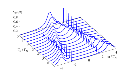
Figure 2: (color online) Particle and hole Fano-type lineshapes appearing at $\pm\varepsilon_{2}$ in the spectral function $\rho_{d1}(\omega)$ of the central quantum dot. Calculations are done for the following parameters $\varepsilon_{1}=0$, $\varepsilon_{2}=2\Gamma_{N}$, $U_{i}=0$, $t=0.2\Gamma_{N}$ and $\Delta=10\Gamma_{N}$.

In the simplest manner a development of the particle and hole interference Fano structures (see Fig. 2) can be explained restricting to the noncorrelated quantum dots. The selfenergies ${\mbox{\boldmath{$\Sigma$}}}_{j}^{0}(\omega)$ are given by

$${\mbox{\boldmath{$\Sigma$}}}_{j}^{0}(\omega)=\!\!\!\sum_{{\bf k},\beta}V_{{\bf k}\beta}\;\;{{\mbox{\boldmath{$g$}}}}_{\beta}({\bf k},\omega)\;V_{{\bf k}\beta}^{*}+t\;{{\mbox{\boldmath{$G$}}}}_{j^{\prime}}(\omega)\;t^{*},$$ (8)

where the inderdot hopping contribution refers to $j^{\prime}\neq j$. The Green’s functions of the conducting leads $\beta=N,D$ have diagonal form

$${{\mbox{\boldmath{$g$}}}}_{\beta}({\bf k},\omega)=\left(\begin{array}[]{cc}\frac{1}{\omega-\xi_{{\bf k}\beta}}&0\\ 0&\frac{1}{\omega+\xi_{{\bf k}\beta}}\end{array}\right)$$ (11)

whereas the superconducting lead is given by the BCS structure

$${{\mbox{\boldmath{$g$}}}}_{S}({\bf k},\omega)=\left(\begin{array}[]{cc}\frac{u^{2}_{\bf k}}{\omega-E_{\bf k}}+\frac{v^{2}_{\bf k}}{\omega+E_{\bf k}}&\frac{-u_{\bf k}v_{\bf k}}{\omega-E_{\bf k}}+\frac{u_{\bf k}v_{\bf k}}{\omega+E_{\bf k}}\\ \frac{-u_{\bf k}v_{\bf k}}{\omega-E_{\bf k}}+\frac{u_{\bf k}v_{\bf k}}{\omega+E_{\bf k}}&\frac{u^{2}_{\bf k}}{\omega+E_{\bf k}}+\frac{v^{2}_{\bf k}}{\omega-E_{\bf k}}\end{array}\right)$$ (14)

with the corresponding coefficients

$$u^{2}_{\bf k},v^{2}_{\bf k} = \frac{1}{2}\left[1\pm\frac{\xi_{{\bf k}S}}{E_{\bf k}}\right]$$

$$u_{\bf k}v_{\bf k} = \frac{\Delta}{2E_{\bf k}},$$

and the quasiparticle energy $E_{\bf k}\!=\!\sqrt{\xi_{{\bf k}S}^{2}+\Delta^{2}}$.

In the wide-band limit we obtain for $\beta=N,D$

$$\sum_{{\bf k}}V_{{\bf k}\beta}\;\;{{\mbox{\boldmath{$g$}}}}_{\beta}({\bf k},\omega)\;V_{{\bf k}\beta}^{*}=-i\frac{\Gamma_{\beta}}{2}\;\left(\begin{array}[]{cc}1&0\\ 0&1\end{array}\right)$$ (17)

and for the superconducting electrode

$$\sum_{{\bf k}}V_{{\bf k}S}\;{{\mbox{\boldmath{$g$}}}}_{S}({\bf k},\omega)\;V_{{\bf k}S}^{*}=-i\frac{\Gamma_{S}}{2}\gamma(\omega)\left(\begin{array}[]{cc}1&\frac{\Delta}{\omega}\\ \frac{\Delta}{\omega}&1\end{array}\right)$$ (20)

with

$$\gamma(\omega)=\frac{|\omega|\;\Theta(|\omega|\!-\!\Delta)}{\sqrt{\omega^{2}-\Delta^{2}}}-\frac{i\omega\;\Theta(\Delta\!-\!|\omega|)}{\sqrt{\Delta^{2}-\omega^{2}}}.$$ (21)

In a far subgap regime $|\omega|\ll\Delta$ only the off-diagonal terms of the matrix (20) are preserved tending to the static value $-\Gamma_{S}/2$. This atomic limit case has been studied by several groups and the results have been recently summarized in the Ref. Yamada-11 . For arbitrary $\Delta$ we obtain the following set of coupled equations

$${\mbox{\boldmath{$G$}}}_{1}(\omega)^{-1} = \left[\omega+i\;\frac{\Gamma_{N}+\gamma(\omega)\Gamma_{S}}{2}\right]{{\mbox{\boldmath{$I$}}}}\!-\!\varepsilon_{1}{{\mbox{\boldmath{$\sigma$}}}}_{z}$$ (22)

$$+\;i\;\frac{\gamma(\omega)\Delta\Gamma_{S}}{2\omega}{{\mbox{\boldmath{$\sigma$}}}}_{y}-|t|^{2}\;{{\mbox{\boldmath{$G$}}}}_{2}(\omega),$$

$${\mbox{\boldmath{$G$}}}_{2}(\omega)^{-1} = \left[\omega+i\;\frac{\Gamma_{D}}{2}\right]{{\mbox{\boldmath{$I$}}}}\!-\!\varepsilon_{2}{{\mbox{\boldmath{$\sigma$}}}}_{z}-|t|^{2}\;{{\mbox{\boldmath{$G$}}}}_{1}(\omega)$$ (23)

where $I$ stands for the identity matrix and ${{\mbox{\boldmath{$\sigma$}}}}_{y,z}$ denote the usual Pauli matrices.

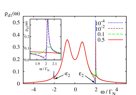
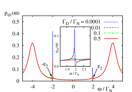
Figure 3: (color online) Spectral function $\rho_{d1}(\omega)$ of the central quantum dot in the equilibrium situation. The upper panel corresponds to $\Gamma_{S}=1.5\Gamma_{N}$ (when the quasiparticle energy $E_{d1}<\varepsilon_{2}$) while the lower one refers to $\Gamma_{S}=8\Gamma_{N}$ (when $E_{d1}>\varepsilon_{2}$). We used for computations the model parameters $\varepsilon_{1}=0$, $\varepsilon_{2}\!=\!2\Gamma_{N}$, $t=0.2\Gamma_{N}$, $U_{i}=0$ and several values of $\Gamma_{D}$.

Figure 2 shows the spectral function $\rho_{d1}(\omega)$ obtained in the equilibrium situation for both uncorrelated quantum dots ($U_{i}\!=\!0$) assuming a weak interdot hopping $t=0.2\Gamma_{N}$ (decoherence is not taken into account here). To focus on the subgap regime $|\omega|\ll\Delta$ we used $\Delta=10\Gamma_{N}$ and other effects related to the gap edge singularities are saparately discussed in the appendix A. For an increasing ratio $\Gamma_{S}/\Gamma_{N}$ we can notice the following qualitative changes: a) the initial lorentzian centered at $\varepsilon_{1}$ splits into two quasiparticle peaks centered at $\pm E_{1}\simeq\pm\sqrt{\varepsilon_{1}+(\Gamma_{S}/2)^{2}}$ (due to the proximity effect), b) the usual Fano-type lineshape formed at $\varepsilon_{2}$ is for larger values of $\Gamma_{S}$ accompanied by appearance of its mirror reflection at $-\varepsilon_{2}$ (we shall refer to these peaks as the particle/hole Fano structures), c) Fano-type lineshapes of these particle/hole features are characterized by an opposite sign of the asymmetry parameter $q$, d) the asymmetry parameters exchange the sign for such $\Gamma_{S}$ when the quasiparticle energy $\sqrt{\varepsilon_{1}^{2}+(\Gamma_{S}/2)^{2}}\!\sim\!\varepsilon_{2}$.

For a closer inspection on the above mentioned changes we examine in the upper (bottom) panel of Fig. 3 the spectral function $\rho_{d1}(\omega)$ obtained for $\Gamma_{S}/\Gamma_{N}=1.5$ ($8$) when $\varepsilon_{2}$ is smaller (larger) than the quasiparticle energy $E_{1}$. We also check the decoherence effect on these particle and hole Fano lineshapes. We notice that already a weak coupling $\Gamma_{D}$ to the floating lead washes out both these particle and hole Fano structures. Thus we conclude that decoherence has a detrimental effect on the quantum interferometric features. To provide some physical argumentation for this behavior let us recall that the resonant level at $\varepsilon_{2}$ gradually broadens uppon increasing $\Gamma_{D}$. For this reason the electron waves are scattered on the side-attached quantum dot without any sharp change of the phase, thereby the Fano-type interference is no longer possible Trocha-12 . In other words, the particle/hole Fano-type lineshapes seem to be rather fragile entities with respect to $\Gamma_{D}$. This remark should be taken into account by experimentalists while constructing the double quantum dot structures on a given substrate material.

IV Andreev spectroscopy

Any practical observation of the interferometric particle/hole Fano lineshapes could be detectable only in the tunneling spectroscopy. For this purpose one could measure e.g. the differential conductance at small bias (i.e. in the subgap regime $|eV|<\Delta$) when charge transport is provided solely via the anomalous Andreev current $I_{A}(V)$. Skipping the details we apply here the popular Landauer-type expression

$$I_{A}(V)=\frac{2e}{h}\int d\omega T_{A}(\omega)\left[f(\omega\!-\!eV,T)\!-\!f(\omega\!+\!eV,T)\right],$$ (24)

derived previously in the Refs Krawiec-04 ; Sun-99 . The Andreev current depends on occupancy $f(\omega\!\pm\!eV,T)$ of the conducting lead (N) convoluted with the transmittance $T_{A}(\omega)$. The latter quantity can be determined from the off-diagonal part of the retarded Green’s function ${{\mbox{\boldmath{$G$}}}}_{1}(\omega)$ via Sun-99 ; Domanski-08

$$T_{A}(\omega)=\Gamma_{N}^{2}\left|G_{1,12}(\omega)\right|^{2}.$$ (25)

The Andreev transmittance (25) is a dimensionless quantity and, roughly speaking, it is a measure of the proximity induced on-dot pairing. Of course (25) depends indirectly on various structures appearing in the spectrum of the central quantum dot, including the particle-hole Fano features.

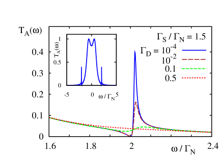
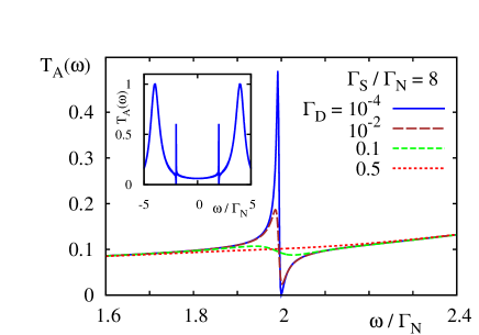
Figure 4: (color online) Andreev transmittance $T_{A}(\omega)$ for the same parameters as in Fig. 3 ($\Gamma_{D}$ is expressed in units of $\Gamma_{N}$).

In particular, the zero-bias differential conductance

$$G_{A}(V\!=\!0)=\frac{4e^{2}}{h}\int d\omega T_{A}(\omega)\left[-\;\frac{df(\omega,T)}{d\omega}\right]$$ (26)

is at low temperatures proportional to the transmittance

$$G_{A}(0)=\frac{4e^{2}}{h}\;T_{A}(\omega\!=\!0),$$ (27)

so the optimal Andreev conductance $4e^{2}/h$ occurs when $T_{A}(\omega)$ reaches the ideal value 1. In figure 4 we plot $\omega$-dependence of the Andreev transmittance for the same set of parameters as discussed in section III. We obtain the symmetric transmittance $T_{A}(-\omega)\!=\!T_{A}(\omega)$ because the anomalous Andreev scattering involves both the particle and hole degrees of freedom. For this reason we notice that at $\omega=\pm\varepsilon_{2}$ there appear the Fano-type structures of identical shapes but characterized by an opposite sign of the asymmetry parameter $q$. Again decoherence proves to have a detrimental influence on both these interferometric structures (compare the curves in Fig. 4 which correspond to several representative values of $\Gamma_{D}$).

V Correlation effects

Let us now consider additional changes of the Fano lineshapes caused by the electron correlations. We shall restrict to the Coulomb repulsion at the side-attached quantum dot $U_{2}$ because the effects of $U_{1}$ have been already studied previously Baranski-11 . Briefly summarizing those studies we can point out that the Coulomb repulsion $U_{1}$ leads to the charging effect and (at low temperatures) can induce the narrow Kondo resonance in the spectrum $\rho_{d1}(\omega)$ for $\omega\sim 0$. The latter effect is experimentally manifested by a slight enhancement of the zero-bias Andreev conductance Deacon_etal . Interference effects (originating from the inter-dot coupling $t$) would qualitatively affect such Kondo feature if $\varepsilon_{2}\sim 0$. Effects of the Fano interference depend also on the ratio $\Gamma_{S}/\Gamma_{N}$ controlling efficiency of the induced on-dot pairing which competes with the Kondo physics Domanski-08 .

So far the correlations have been intensively studied mainly for the case of single quantum dot coupled between the metallic and superconducting electrodes Rodero-11 . For this purpose there have been adopted various many-body techniques, such as: the mean field slave boson approach Fazio-98 , noncrossing approximation Clerk-00 , iterated perturbative scheme Cuevas-01 ; Yamada-11 , modified slave boson method Krawiec-04 , numerical renormalization group calculations Tanaka-07 ; Bauer-07 ; Hecht-08 and other Sun-99 ; Cho-99 ; Avishai-01 ; Domanski-08 ; Paaske-10 . The interests focused predominantly on an interplay between the on-dot pairing and the Kondo state Yamada-11 . It has been experimentally proved Deacon_etal that such interrelation is governed by the ratio $\Gamma_{S}/\Gamma_{N}$. For $\Gamma_{S}\gg\Gamma_{N}$ the on-dot pairing plays a dominant role (suppressing or completely destroying the Kondo resonance). In the opposite regime $\Gamma_{S}\ll\Gamma_{N}$ the Kondo state is eventually observed (coupling $\Gamma_{N}$ to the normal lead is necessary for that).

In this section we study the role of correlations $U_{2}$ in the side-coupled quantum dot taking also into account decoherence caused by the floating lead. For simplicity we shall neglect the impact of $U_{2}$ on the off-diagonal parts of ${{\mbox{\boldmath{$G$}}}}_{2}(\omega)$ because the pairing induced in QD₂ for small interdot hopping $t$ can be anyhow expected to be marginal. Thus we determine the Green’s function ${{\mbox{\boldmath{$G$}}}}_{2}(\omega)$ from the Dyson equation (4) imposing the diagonal selfenergy

$$\Sigma^{e-e}_{2}(\omega)\simeq\left(\begin{array}[]{cc}\Sigma_{N}(\omega)&0\\ 0&-\left[\Sigma_{N}(-\omega)\right]^{*}\end{array}\right).$$ (30)

Formally $\Sigma_{N}(\omega)$ denotes the selfenergy of the Anderson impurity immersed in the normal Fermi liquid. Obviously such selfenergy is not known exactly Hewson therefore we have to invent some approximations.

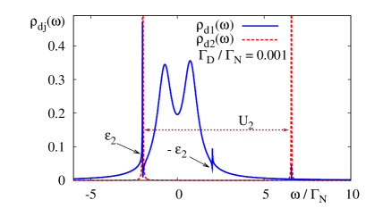
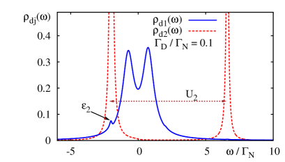
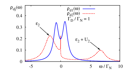
Figure 5: (color online) Evolution of the Fano-type lineshapes for several couplings $\Gamma_{D}$ as indicated. Calculations have been done for $T=0.001\Gamma_{N}$ (lower than $T_{K}$), using the model parameters $\varepsilon_{1}=0$, $\varepsilon_{2}=-2\Gamma_{N}$, $t=0.2\Gamma_{N}$, $\Gamma_{S}=1.5\Gamma_{N}$ and assuming the large superconducting gap $\Delta=10\Gamma_{N}$.

Among possible choices we adopt the equation of motion method EOM which is capable to reproduce qualitatively the Coulomb blockade and the Kondo effects. Besides its simplicity this method is however not very precise with regard to the low energy structure of the Kondo peak $\rho_{d2}(\omega\sim 0)=\frac{2}{\pi\Gamma_{D}}\frac{T_{K}^{2}}{\omega^{2}+T_{K}^{2}}$. Nevertheless our results might give some hints on the qualitative trends and quality of this information could be improved using more sophisticated tools. Skipping technicalities discussed by us in the appendix B of Ref. Baranski-11 we can express the selfenergy $\Sigma_{N}(\omega)$ through

$$\left[\omega\!-\!\varepsilon_{2}\!-\!\Sigma_{N}(\omega)\right]^{-1}=$$ (31)

$$\frac{\tilde{\omega}-\varepsilon_{2}-[\Sigma_{N3}(\omega)+U_{2}(1\!-\!\langle\hat{n}_{2\downarrow}\rangle)]}{[\tilde{\omega}\!-\!\varepsilon_{2}][\tilde{\omega}\!-\!\varepsilon_{2}\!-\!U_{2}\!-\!\Sigma_{N3}(\omega)]\!+\!U_{2}\Sigma_{N1}(\omega)}$$

where $\tilde{\omega}\!=\!\omega\!-\!\sum_{\bf k}|V_{{\bf k}D}|^{2}/(\omega\!-\!\xi_{{\bf k}D})\!\simeq\!\omega+\frac{i\Gamma_{D}}{2}$. The other symbols are defined as follows $\Sigma_{N1}(\omega)\!=\!\sum_{\bf k}|V_{{\bf k}D}|^{2}f(\xi_{{\bf k}D},T)[(\omega\!-\!\xi_{{\bf k}D})^{-1}+(\omega\!-\!U_{2}\!-2\varepsilon_{2}\!+\!\xi_{{\bf k}D})^{-1}]$ and $\Sigma_{N3}(\omega)\!=\!\sum_{\bf k}|V_{{\bf k}D}|^{2}[(\omega\!-\!\xi_{{\bf k}D})^{-1}+(\omega\!-\!U_{2}\!-2\varepsilon_{2}\!+\!\xi_{{\bf k}D})^{-1}]$. This expression (31) for $\Sigma_{N}(\omega)$ substituted to the selfenergy (30) yields the Green’s function ${{\mbox{\boldmath{$G$}}}}_{1}(\omega)$ of the central quantum dot via the exact relation (22). In this way we can numerically determine the effect of $U_{2}$ on $\rho_{d1}(\omega)$ and on the Andreev transport.

For a weak interdot hopping $t$ (which is necessary to allow for the Fano-type quantum interference) we notice that the correlations $U_{2}$ can be manifested in the spectral function $\rho_{d1}(\omega)$ by i) the charging effect and ii) another characteristic structure due to the Kondo effect.

i) The first effect can be observed only if a decoherence is sufficiently weak, strictly speaking for $\Gamma_{D}\leq 0.1\Gamma_{N}$. Under such circumstances the particle and hole Fano lineshapes (at $\pm\varepsilon_{2}$) are accompanied by two additional Coulomb satellites at $\pm(\varepsilon_{2}+U_{2})$. These interferometric features (see the top and middle panels of Fig. 5) are completely washed out from the spectrum when $\Gamma_{D}$ slightly exceeds the value $0.1\Gamma_{N}$. This destructive effect of a decoherence resembles the behavior discussed in section III (see Fig.  3) for the case of uncorrelated quantum dots.

ii) Instead of the particle/hole Fano lineshapes and their Coulomb satellites we can eventually observe a different qualitative structure at $\omega\sim 0$ when the coupling $\Gamma_{D}$ is large (provided that temperature $T<T_{K}(\Gamma_{D})$. Its appearance is related to the Kondo resonance formed at the side-attached quantum dot (see the dashed curve in the bottom panel of Fig. 5). Due to the inderdot hopping $t$ the mentioned Kondo resonance affects the central quantum dot in pretty much the same way as did the narrow resonant level $\varepsilon_{2}$ in a weak coupling regime $\Gamma_{D}$. Consequently we thus again observe the tiny Fano lineshape in the spectral function $\rho_{d1}(\omega)$ of the central quantum dot and in the Andreev transmittance $T_{A}(\omega)$ near $\omega\sim 0$.

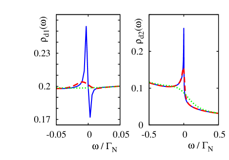
Figure 6: (color online) Influence of the Kondo effect appearing in $\rho_{d2}(\omega)$ on a tiny Fano-type structure of the central quantum dot spectrum $\rho_{d1}(\omega)$ near $\omega=0$. The curves have been calculated using the same parameters as in figure 5 for the following temperatures $T/\Gamma_{N}=0.001$ (solid line), $0.01$ (dashed line) and $0.1$ (dotted line).

Since the Kondo-induced interferometric structure is hardly noticeable on the large energy scale we show it separately in Fig. 6 restricting to a narrow regime around the Fermi level $\omega=0$. Let us remark that the Kondo resonance in $\rho_{d2}(\omega)$ and its Fano-type manifestation in $\rho_{d1}(\omega)$ are both very sensitive to temperature. This fact proves that the considered Fano lineshape at $\omega\sim 0$ is intimately related to the Kondo effect on the side-attached quantum dot.

VI Conclusions

In summary, we have investigated the influence of decoherence and electron correlations on the interferometric Fano-type lineshapes of the double quantum dot coupled in T-shape configuration to the conducting and superconducting leads. We find evidence that already a weak decoherence can consequently smear out the Fano lineshapes of the particle and hole states. On a microscopic level this detrimental influence can be assigned to a broadening of the resonant levels near $\pm\varepsilon_{2}$, so that the phase shift of the scattered electron waves is no longer sharp and therefore the Fano-type interference cannot be satisfied Miroshnichenko-10 .

The correlations $U_{2}$ on the side-attached quantum dot have the additional qualitative influence. For a weak decoherence the particle/hole Fano structures at $\pm\varepsilon_{2}$ are accompanied by appearance of their Coulomb satellites at $\pm(\varepsilon_{2}+U_{2})$. All these interferometric features gradually disappear upon increasing $\Gamma_{D}$ (i.e. for stronger decoherence). On the other hand, in the opposite regime of strong coupling $\Gamma_{D}$, the narrow Kondo resonance appears in the spectral function $\rho_{d2}(\omega)$ of the side-coupled quantum dot. Its formation gives rise to the new interferometric structure appearing in the spectrum of the central quantum dot at $\omega\sim 0$. This temperature dependent Fano-type lineshape is observable in the spectral function $\rho_{d1}(\omega)$ and would be detectable in the Andreev conductance. Such Kondo-induced Fano effect is however very tiny therefore its experimental verification might be challenging.

Appendix A Gap edge features

There is also another important energy scale, relevant for the present study. It is related to a magnitude of the energy gap $\Delta$ of superconducting lead. To illustrate its influence on the spectral function $\rho_{d1}(\omega)$ we show in figure 7 variation within the region $0\leq\Delta\leq 4\Gamma_{N}$. If the energy gap is small we see that the proximity effect is very fragile. For this reason we hardly notice the Fano-type structure at $-\varepsilon_{2}$ because the on-dot pairing is rather ineffective. The Fano resonance starts to be well pronounced at $-\varepsilon_{2}$ when $\Delta$ becomes comparable (or larger) than $\Gamma_{S}$. Additionally, the energy gap $\Delta$ is responsible for two tiny dips appearing at $\omega=\pm\Delta$. They are signatures of the gap edge singularities of superconducting lead. Roughly speaking, outside the energy regime $|\omega|>\mbox{\rm min}\left\{\Delta,\Gamma_{S}/2\right\}$ the charge tunneling occurs via the usual single particle channel and the Andreev tunneling is there no longer dominant Fazio-98 ; Clerk-00 ; Cuevas-01 ; Krawiec-04 ; Sun-99 ; Domanski-08 .

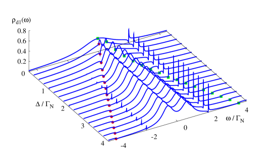
Figure 7: (color online) Evolution of the particle/hole Fano lineshapes at $\pm\varepsilon_{2}$ obtained for $\varepsilon_{1}=0$, $\varepsilon_{2}=2\Gamma_{N}$, $t=0.2\Gamma_{N}$, $\Gamma_{S}=1.5\Gamma_{N}$, $U_{i}=0$ and for the varying magnitude of $\Delta$. The filled circles and squares indicate the cusp-like signatures of the gap edge singularites at $-\Delta$ and $+\Delta$.

References

- (1) A. Martin-Rodero and A. Levy-Yeyati, Adv. Phys. 60, 899 (2011).
- (2) R.S. Deacon, Y. Tanaka, A. Oiwa, R. Sakano, K. Yoshida, K. Shibata, K. Hirakawa, and S. Tarucha, Phys. Rev. Lett. 104, 076805 (2010); R.S. Deacon, Y. Tanaka, A. Oiwa, R. Sakano, K. Yoshida, K. Shibata, K. Hirakawa, and S. Tarucha, Phys. Rev. B 81, 121308(R) (2010).
- (3) J.-D. Pillet, C.H.L. Quay, P. Morfin, C. Bena, A. Levy-Yeyati, and P. Joyez, Nature Phys. 6, 965 (2010).
- (4) R. Maurand, T. Meng, E. Bonet, S. Florens, L. Marty, and W. Wernsdorfer, Phys. Rev. X 2, 011009 (2012).
- (5) H.I. Jorgensen, K. Grove-Rasmussen, T. Novotny, K. Flensberg, and P.E. Lindelof, Phys. Rev. Lett. 96, 207003 (2006).
- (6) J.A. van Dam, Yu.V. Nazarov, E.P.A.M. Bakkers, S. De Franceschi, L.P. Kouwenhoven, Nature 442, 667 (2006).
- (7) J.-P. Cleuziou, W. Wernsdorfer, V. Bouchiat, T. Ondarcuhu, and M. Monthioux, Nature Nanotechnology 1, 53 (2006).
- (8) W.-Z. Gao, W.-J. Gong, Y.-S. Zheng, Y. Liu, and T.-Q. Lü, Commun. Theor. Phys. (Beijing) 49, 771 (2008).
- (9) R. Žitko, Phys. Rev. B 81, 115316 (2010).
- (10) Y. Tanaka, N. Kawakami, and A. Oguri, Phys. Rev. B 78, 035444 (2008); J. Phys.: Conf. Series 150, 022086 (2009).
- (11) Y. Yamada, Y. Tanaka, and N. Kawakami, J. Phys. Soc. Jpn. 79, 043705 (2010); Y. Tanaka, N. Kawakami, and A. Oguri, Phys. Rev. B 81, 075404 (2010).
- (12) J. Barański and T. Domański, Phys. Rev. B 84, 195424 (2011).
- (13) A.E. Miroshnichenko, S. Flach, and Y.S. Kivshar, Rev. Mod. Phys. 82, 2257 (2010).
- (14) P. Trocha, J. Phys.: Condens. Matter 24, 055303 (2012).
- (15) S. Sasaki, H. Tamura, T. Akazaki, and T. Fujisawa, Phys. Rev. Lett. 103, 266806 (2009).
- (16) K. Kobayashi, H. Aikawa, A. Sano, S. Katsumoto, and Y. Iye, Phys. Rev. B 70, 035319 (2004).
- (17) V. Madhavan, W. Chen, T. Jamneala, M.F. Crommie, and N.S. Wingreen, Phys. Rev. B 64, 165412 (2001).
- (18) C. Fühner, U.F. Keyser, R.J. Haug, D. Reuter, and A.D. Wieck, Phys. Rev. B 66, 161305 (2002).
- (19) P. Stefański, A. Tagliacozzo, and B.R. Bułka, Phys. Rev. Lett. 93, 186805 (2004); W. Hofstetter, J. König, and H. Schoeller, Phys. Rev. Lett. 87, 156803 (2001); B. Bułka, P. Stefański, Phys. Rev. Lett. 86, 5128 (2001).
- (20) A. Grigoriev, J. Sköldberg, G. Wendin, and Z. Crljen, Phys. Rev. B 74, 045401 (2006).
- (21) A.R. Schmidt, M.H. Hamidian, P. Wahl, F. Meier, A.V. Balatsky, J.D. Garrett, T.J. Williams, and G.M. Luke, Nature 465, 570 (2010).
- (22) L.E. Calvet, J.P. Snyder, and W. Wernsdorfer, Phys. Rev. B 83, 205415 (2011).
- (23) Y. Yamada, Y. Tanaka, and N. Kawakami, Phys. Rev. B 84, 075484 (2011).
- (24) R. Fazio and R. Raimondi, Phys. Rev. Lett. 80, 2913 (1998); Phys. Rev. Lett. 82, 4950 (1999); P. Schwab and R. Raimondi, Phys. Rev. B 59, 1637 (1999).
- (25) A.A. Clerk, V. Ambegaokar, and S. Hershfield, Phys. Rev. B 61, 3555 (2000).
- (26) J.C. Cuevas, A. Levy Yeyati, and A. Martin-Rodero, Phys. Rev. B 63, 094515 (2001).
- (27) M. Krawiec and K.I. Wysokiński, Supercond. Sci. Technol. 17, 103 (2004).
- (28) Y. Tanaka, N. Kawakami, and A. Oguri, J. Phys. Soc. Jpn. 76, 074701 (2007).
- (29) J. Bauer, A. Oguri, and A.C. Hewson, J. Phys.: Condens. Matter 19, 486211 (2007).
- (30) T. Hecht, A. Weichselbaum, J. von Delft, and R. Bulla, J. Phys. Condens. Matter 20, 275213 (2008).
- (31) Q.-F. Sun, J. Wang, and T.-H. Lin, Phys. Rev. B 59, 3831 (1999); Q.-F. Sun, H. Guo, and T.-H. Lin, Phys. Rev. Lett. 87, 176601 (2001).
- (32) S.Y. Cho, K. Kang, and C.-M. Ryu, Phys. Rev. B 60, 16874 (1999).
- (33) Y. Avishai, A. Golub, and A.D. Zaikin, Phys. Rev. B 63, 134515 (2001); T. Aono, A. Golub, and Y. Avishai, Phys. Rev. B 68, 045312 (2003).
- (34) T. Domański and A. Donabidowicz Phys. Rev. B 78, 073105 (2008); T. Domański, A. Donabidowicz, and K.I. Wysokiński, Phys. Rev. B 78, 144515 (2008); Phys. Rev. B 76, 104514 (2007).
- (35) V. Koerting, B.M. Andersen, K. Flensberg, and J. Paaske, Phys. Rev. B 82, 245108 (2010).
- (36) A.C. Hewson, The Kondo problem to heavy fermions Cambridge University Press, Cambridge (1993).
- (37) H. Haug and A.-P. Jauho, Quantum Kinetics in Transport and Optics of Semiconductors, Springer Verlag, Berlin (1996).