Gamma-expansion for a 1D Confined Lennard-Jones model with point defect

Abstract.

We compute a rigorous asymptotic expansion of the energy of a point defect in a 1D chain of atoms with second neighbour interactions. We propose the Confined Lennard-Jones model for interatomic interactions, where it is assumed that nearest neighbour potentials are globally convex and second neighbour potentials are globally concave. We derive the $\Gamma$-limit for the energy functional as the number of atoms per period tends to infinity and derive an explicit form for the first order term in a $\Gamma$-expansion in terms of an infinite cell problem. We prove exponential decay properties for minimisers of the energy in the infinite cell problem, suggesting that the perturbation to the deformation introduced by the defect is confined to a thin boundary layer.

1. Introduction

The analysis of discrete lattice systems and their relationship to continuum mechanics is currently a growing area of study within applied analysis. Many rigorous results have been obtained in the past ten years connecting discrete models with continuum limits, which are extensively surveyed in [BLBL07]. The most well-developed approaches have been either to apply $\Gamma$-convergence to discrete energy functionals parametrised by the number of atoms per unit volume in the model (see [Sch06, AC04, BG02]), or to apply forms of the inverse function theorem to show that for a discrete energy with the same parameter fixed, the Cauchy–Born rule holds; i.e. for a given atomistic deformation and a certain range of atomic densities there exist continuum deformations which are close in some norm, and have a similar energy (see [OT12, EM07]).

Here, we take the former approach. We build upon recent works on surface energies in discrete systems [SSZ11, BC07], which employ ‘$\Gamma$-development’ as first defined in [AB93], and extensively discussed in [BT08]. We define energy functionals with and without defects, and present the Confined Lennard-Jones model for interatomic interactions, which we motivate with a formal analysis. We then investigate the scaling of the perturbation to the energy which is introduced by the defect. We also provide a concrete cell problem that may be used for explicit computation of the first-order energy, and show that a minimiser of this cell problem decays exponentially away from the defect. This allows us to conclude that minimisers of the energies with and without a defect are essentially the same except on a thin boundary layer around the defect.

1.1. Motivation

The tools developed to study the relationship between atomistic and continuum models rely upon the high level of symmetry which is maintained after deforming a crystal. However, the pure lattice behaviour is not the only factor in determining the bulk properties of such materials. The last century saw a revolution in the materials science community, as it was realised that lattice defects can change the strength of an otherwise perfect crystal by orders of magnitude. Understanding defects, how they scale and in what rigorous ways one might modify the continuum approximation of crystalline solids to take them into account is therefore key to developing our understanding of how best to model and predict their behaviour.

As a first step towards this goal, we consider arguably the simplest crystalline defect, a dilute point defect. A point defect is an interruption of the pure lattice structure caused by changing an atom at some lattice site (called an impurity) or by inserting an atom into the structure at a point which is not a lattice site (called an interstitial). In 1D, impurities and interstitials are essentially identical when atoms are treated as point particles with hard-core interactions, since atoms cannot move past one another, and so it is easy to modify the reference configuration to take such a defect into account. In higher dimensions, the two defects are qualitatively different (see Figure 1), with an interstitial requiring an additional point in the reference configuration which breaks the symmetry.

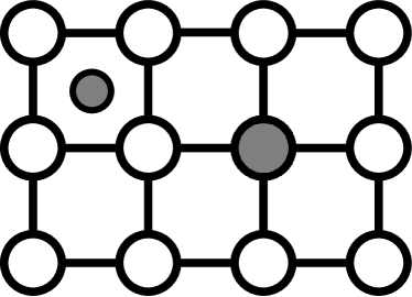
(a) 2D Defects

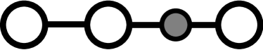
(b) 1D Defect

Figure 1. Impurities and Interstitials.

The model we analyse is one-dimensional, and to avoid surface effects, we use a periodic reference domain, so that in effect the atoms lie on a one-dimensional torus. The defect considered is dilute since only one atom in the chain is of a different type.

By computing the $\Gamma$-limit of the sequence of energy functionals for the model described here, we arrive at an energy which encodes some of the properties of the minimisers of the functionals along the sequence, but no quantitative information about the error made. Computing higher-order limits gives further, more quantitative control on the energy minima, and in this case will also allow us to say something more qualitative about the minimisers.

1.2. Outline

As discussed above, we apply $\Gamma$-convergence to a sequence of atomistic energy functionals that depend on the parameter $\varepsilon$, which is the inverse of the number of atoms per unit volume.

In the remainder of Section 1, we propose a model for interatomic interactions in a 1D chain including a point defect. We then make a formal analysis of the model to motivate this study and the Confined Lennard-Jones model which we propose, before reformulating the problem in a format amenable to analysis in the framework of the one-dimensional Calculus of Variations.

In Section 2, we derive the $\Gamma$-limit for the series of functionals defined in Section 1 as $\varepsilon$ tends to zero, and note that the introduction of the defect does not perturb the $\Gamma$-limit at this order.

In Section 3, we collect and prove some results about the minimum problem for the $0^{\text{th}}$-order $\Gamma$-limit of the atomistic energies, including existence, uniqueness and regularity for minimisers.

In Section 4, we proceed to derive a first-order $\Gamma$-limit, expressing it in terms of a minimisation problem in an infinite cell, and prove some properties of this minimum problem along the way.

1.3. Physical model

For now, fix $N\in\mathbb{N}$. We consider $2N$ atoms indexed by

$$i\in\{-N,\ldots,N-1\}$$

which have a spatial density of $2N/L$, where $L$ is the total length of the deformed configuration. To make the domain periodic, we identify an atom indexed by $i=N$ with the atom $i=-N$ so that we avoid boundary effects, and defining $\varepsilon=1/2N$, we choose to take reference positions for these atoms to be

$$x_{i}:=i\varepsilon\in\Omega_{\varepsilon}:=\big{\{}-{\textstyle\frac{1}{2}},-{\textstyle\frac{1}{2}}+\varepsilon,\ldots,{\textstyle\frac{1}{2}}\big{\}}.$$

We also define

$$\Omega:=[-{\textstyle\frac{1}{2}},{\textstyle\frac{1}{2}}],$$

so that $\Omega_{\varepsilon}=\Omega\cap\varepsilon\mathbb{Z}$. It should be noted at the outset that the choice to use $2N$ atoms will not be restrictive to our analysis but will make some of the concepts easier to elucidate, and that we will frequently write $\varepsilon\rightarrow 0$ to mean $N\rightarrow\infty$.

Fixing the coordinate system so that atom $-N$ lies at $0$, any configuration can be described by a map

$$y:\Omega_{\varepsilon}\rightarrow[0,L]\qquad\text{such that}\qquad y(-{\textstyle\frac{1}{2}})=0,y({\textstyle\frac{1}{2}})=L.$$

We will use the shorthand

$$y_{i}:=y(x_{i}),$$

and extend $y$ to a map on the whole of $\varepsilon\mathbb{Z}$ by defining

$$y_{2kN+i+1}-y_{2kN+i}:=y_{i+1}-y_{i}$$

for any $k\in\mathbb{Z}$.

The atoms in our model are assumed to interact through pair potentials which decay rapidly so that it suffices to consider an interaction between atoms and their 2 immediate neighbours on either side. As explained in Section 1.1, all atoms except one are of the same type, regarded as the ‘pure’ species. As in [BDMG99], the potential energy of a bond between atoms is assumed to be expressed as a function of the relative displacement

$$D_{j}y_{i}:=\frac{y_{i+j}-y_{i}}{x_{i+j}-x_{i}}=\frac{y_{i+j}-y_{i}}{j\varepsilon}.$$

In the case where all atoms are of the pure species, a bond with relative length $s$ has energy $\phi_{1}(t)$ for nearest neighbours, and $\phi_{2}(t)$ for second neighbours. The internal energy of the configuration arising from the interatomic forces is

$$E^{\varepsilon}_{\rm p}(y):=\sum_{i=-N}^{N-1}\phi_{1}(D_{1}y_{i})+\phi_{2}(D_{2}y_{i}).$$

Since in each configuration we assume there is a single defect, we assume without loss of generality that the defect is at index $i=0$. The energy of bonds of relative length $s$ between this atom and its neighbours are $\psi_{1}(t)$ for the nearest neighbours and $\psi_{2}(t)$ for second neighbours (see Figure 2).

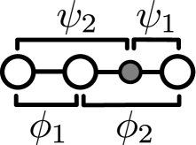
Figure 2. Pair Potentials

The introduction of the defect causes a modification of the energy which is given by the addition of the following energy term:

$$E_{\rm d}(y):=\psi_{2}(D_{2}y_{-2})-\phi_{2}(D_{2}y_{-2})+\psi_{1}(D_{1}y_{-1})-\phi_{1}(D_{1}y_{-1})$$

$$+\psi_{1}(D_{1}y_{0})-\phi_{1}(D_{1}y_{0})+\psi_{2}(D_{2}y_{0})-\phi_{2}(D_{2}y_{0}).$$

Finally, we also consider dead loads $f_{i}$ acting on each atom. Taking as initial positions the points $L(x_{i}+{\textstyle\frac{1}{2}})$, the work done by these forces is

$$E^{\varepsilon}_{\rm f}(y):=\sum_{i=-N}^{N-1}f_{i}\big{(}y_{i}-L(x_{i}+{\textstyle\frac{1}{2}})\big{)}.$$

This term can be though of as the work done by a linearisation of some external force field near the homogeneous linear state $y_{i}=L(x_{i}+{\textstyle\frac{1}{2}})$. To keep notation concise, we will frequently write $u_{i}$ to mean

$$u_{i}:=y_{i}-L(x_{i}+{\textstyle\frac{1}{2}}),$$

and we extend $f$ by periodicity to a map over $\varepsilon\mathbb{Z}$ by defining

$$f_{2kN+i}=f_{i}$$

for any $k\in\mathbb{Z}$.

The total energy for the atomistic system considered is therefore

$$E^{\varepsilon}(y):=E^{\varepsilon}_{\rm p}(y)+E_{\rm d}(y)+E^{\varepsilon}_{\rm f}(y).$$

1.4. Formal analysis

We expect that atoms should minimise the energy $E^{\varepsilon}$, and we therefore seek to characterise the minimal energy and the states which attain this minimum. We will consider the situation when $N$ is large, and when the material is behaving elastically. In this case, interatomic displacements should vary slowly over the domain, and so we assume the Cauchy–Born hypothesis holds (for more information, see [Zan96]). This states that interatomic displacements follow linear deformations of small volumes of the solid, and so we assume that

$$D_{1}y_{i},D_{2}y_{i} \simeq Dy(x_{i}),$$

where $y:\Omega\rightarrow[0,L]$ is some suitably smooth function describing the displacement. This means that the energy

$$\phi_{1}(D_{1}y_{i})+\phi_{2}(D_{2}y_{i}) \simeq\phi_{1}\big{(}Dy(x_{i})\big{)}+\phi_{2}\big{(}Dy(x_{i})\big{)}.$$

Motivated by this we define $W$, the continuum elastic energy density to be

$$W(t):=\phi_{1}(t)+\phi_{2}(t).$$ (1.1)

The total energy is now approximately

$$E^{\varepsilon}(y) \simeq\sum_{i=-N}^{N-1}W(Dy(x_{i}))+E_{\rm d}(y)+E^{\varepsilon}_{\rm f}(y).$$

We expect this energy to grow linearly as the number of atoms increases, so it makes sense to look at the mean energy per atom, $\varepsilon E^{\varepsilon}$, as $N$ gets large. The size of the defect is fixed and small, so $\varepsilon E_{\rm d}(y)$ should vanish as $\varepsilon\rightarrow 0$, and

$$\varepsilon E^{\varepsilon}(y) \simeq\varepsilon\sum_{i=-N}^{N-1}W\big{(}Dy(x_{i})\big{)}+f_{i}u_{i}$$

$$\simeq\mathcal{F}_{0}(y):=\int_{\Omega}W(Dy)+fu\,{\rm d}x,$$

where $u(x)=y(x)-L(x+{\textstyle\frac{1}{2}})$. The minimiser of the right hand side should satisfy the Euler–Lagrange equation for this functional,

$${\textstyle\frac{\rm d}{\,{\rm d}x}}\big{(}W^{\prime}(Dy)\big{)}=f(x).$$

This equation can be integrated to give

$$W^{\prime}(Dy)=\sigma(x)+\Sigma,\qquad\text{where}\qquad\sigma(x)=\int_{-1/2}^{x}f(t)\,{\rm d}t.$$

The defect should then contribute a further term proportional to its size, $O(\varepsilon)$, to the energy. Since the mean energy is only perturbed by a small amount, we should expect that any perturbation to the minimiser would also occur close to the defect, due to the mismatch between $\phi_{i}$ and $\psi_{i}$ there. The defect always remains at $i=0$, so when $N$ is large, we make the ansatz that close to the defect $D_{1}y_{i}\simeq F_{0}+r_{i}$, where $F_{0}:=Dy(0)$ and $r_{i}$ is a small perturbation. Defining

$$\sigma^{\varepsilon}_{-N} :=-{\textstyle\frac{1}{2}}\varepsilon f_{-N}\qquad\text{and}\qquad\sigma^{\varepsilon}_{i}:=\sigma^{\varepsilon}_{i-1}+\varepsilon f_{i-1},$$

then integrating by parts, we can rewrite the external force terms as

$$\sum_{i=-N}^{N-1}f_{i}u_{i}=\sum_{i=-N}^{N-1}\sigma^{\varepsilon}_{i}\,D_{1}u_{i}\quad\text{and}\quad\int_{\Omega}fu\,{\rm d}x=\int_{\Omega}\sigma\,Du\,{\rm d}x.$$

This then means the additional contribution is

$$\frac{\varepsilon E^{\varepsilon}(y)-\mathcal{F}_{0}(y)}{\varepsilon}\simeq\tilde{E}_{\infty}(r):=\tilde{E}_{\rm d}(r)+\sum_{i=-\infty}^{\infty}\Big{(}\phi_{1}\big{(}F_{0}+r_{i}\big{)}+\phi_{2}\big{(}F_{0}+{\textstyle\frac{r_{i}+r_{i+1}}{2}}\big{)}-W(F_{0})\\ +\sigma_{i}\big{(}F_{0}+r_{i}-L\big{)}-\sigma(0)\big{(}F_{0}-L\big{)}\Big{)},$$

where we have defined

$$E_{\rm d}(r):=\psi_{2}(F_{0}+{\textstyle\frac{r_{-2}+r_{-1}}{2}})-\phi_{2}(F_{0}+{\textstyle\frac{r_{-2}+r_{-1}}{2}})+\psi_{1}(F_{0}+r_{-1})-\phi_{1}(F_{0}+r_{-1})\\ +\phi_{1}(F_{0}+r_{0})-\psi_{1}(F_{0}+r_{0})+\psi_{2}(F_{0}+{\textstyle\frac{r_{0}+r_{1}}{2}})-\phi_{2}(F_{0}+{\textstyle\frac{r_{0}+r_{1}}{2}}).$$

If $f$ is smooth enough, then for $i$ close to $0$ and $\varepsilon$ small, $\sigma^{\varepsilon}_{i}\simeq\sigma(0)$, so the integrated Euler–Lagrange equation for $\mathcal{F}_{0}$ gives

$$\tilde{E}_{\infty}(r)\simeq E_{\rm d}(r)+\sum_{i=-\infty}^{\infty}\phi_{1}\big{(}F_{0}+r_{i}\big{)}+\phi_{2}\big{(}F_{0}+{\textstyle\frac{r_{i}+r_{i+1}}{2}}\big{)}-W(F_{0})-\big{(}W^{\prime}(F_{0})-\Sigma\big{)}r_{i}.$$

The sum of the $\Sigma\,r_{i}$ terms should vanish due to the boundary conditions. Since we expect decaying solutions, we linearise in $r_{i}$ away from the defect, giving

$$\tilde{E}_{\infty}(r)\simeq E_{c}(y)+{\textstyle\frac{1}{2}}\sum_{|i|\geq R}\phi_{1}^{\prime\prime}(F_{0})r_{i}^{2}+\phi_{2}^{\prime\prime}(F_{0})\big{(}{\textstyle\frac{r_{i}+r_{i+1}}{2}}\big{)}^{2}.$$

For a minimiser of this energy, the $r_{i}$ should approximately satisfy

$${\textstyle\frac{1}{2}}\phi_{2}^{\prime\prime}(F_{0})(r_{i-1}+r_{i})+\phi_{1}^{\prime\prime}(F_{0})r_{i}+{\textstyle\frac{1}{2}}\phi_{2}^{\prime\prime}(F_{0})(r_{i}+r_{i+1})=0.$$

Making the usual ansatz $r_{i}=a\lambda^{i}$, a solution must satisfy

$${\textstyle\frac{1}{2}}\phi_{2}^{\prime\prime}(F_{0})+W^{\prime\prime}(F_{0})\lambda+{\textstyle\frac{1}{2}}\phi_{2}^{\prime\prime}(F_{0})\lambda^{2}=0.$$

If $\phi_{1}$ and $W$ are convex and $\phi_{2}$ is concave at $F_{0}$, as is the case in Lennard-Jones type pair potentials, then a straightforward analysis of the roots of this equation implies that there are two positive real roots which multiply to give $1$. These two roots correspond to an exponentially decaying solution and an exponentially growing solution.

Rigorous versions of these formal results will be the subject of this paper, and motivate the assumptions we make about the potentials and external force in the following section.

1.5. Confined Lennard-Jones Model

Motivated by the formal analysis carried out in the previous section, this section details the assumptions that we make about the pair potentials and external force field.

We will assume that all potentials $\phi_{i}$ and $\psi_{i}$ are ${\rm C}^{2}$ on the interval $(0,\infty)$. Additionally, we assume the potentials and external forces satisfy the following conditions.

1. The nearest neighbour potentials are infinite for negative bond lengths and blow up as bond lengths approach zero, i.e.

   $$\phi_{1}(t),\psi_{1}(t) =+\infty\text{ for }s\leq 0,$$

   $$\lim_{s\searrow 0}\phi_{1}(t)=+\infty\quad \text{and}\quad\lim_{s\searrow 0}\psi_{1}(t)=+\infty.$$

2. The nearest neighbour potentials are $l$-convex, i.e. for any $s>0$,

   $$\phi_{1}^{\prime\prime}(t),\psi_{1}^{\prime\prime}(t)\geq l>0.$$

3. The second neighbour potentials $\phi_{2}$ and $\psi_{2}$ are concave.

4. The second neighbour potentials $\phi_{2}$ and $\psi_{2}$ are ‘dominated’ by the nearest neighbour potentials $\phi_{1}$ and $\psi_{1}$, i.e. there exist constants $\alpha\in(0,1)$ and $C\in\mathbb{R}$ such that

   $$\phi_{2}(x) \geq-\alpha\,\phi_{1}(x)+C, \phi_{2}(x) \geq-\alpha\,\psi_{1}(x)+C,$$

   $$\psi_{2}(x) \geq-\alpha\,\phi_{1}(x)+C, \psi_{2}(x) \geq-\alpha\,\psi_{1}(x)+C.$$

5. The ‘pure’ potentials are such that the resulting continuum elastic potential is $l$-convex, i.e. defining $W$ as in (1.1), for any $t>0$,

   $$W^{\prime\prime}(t)=\phi_{1}^{\prime\prime}(t)+\phi_{2}^{\prime\prime}(t)\geq l.$$

6. We assume $f_{i}=f(x_{i})$ where $f\in{\rm C}^{2}(\Omega)$.

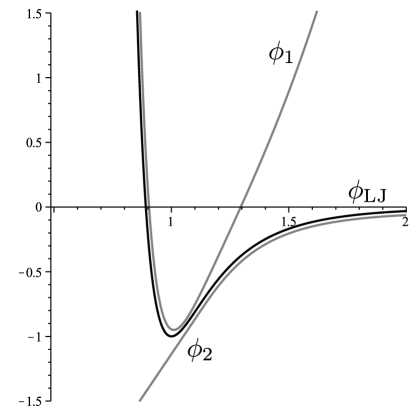
Figure 3. Possible choices of $\phi_{1}$ and $\phi_{2}$ with the assumptions prescribed which approximate a Lennard-Jones potential, $\phi_{\mathrm{LJ}}$.

Remark 1. Assumption (1) prevents atoms from exchanging positions with respect to the reference configuration, and ensures that we prevent plastic deformation.

Assumptions (2) and (3) are made to simulate the behaviour of a Lennard-Jones type potential, which is convex for short bond lengths, and then concave after for any bond length past some critical length; see for example Figure 3. When under strains in the elastic regime, the nearest neighbours lie in the convex part of the potential, and all other atoms lie in the concave part.

Assumption (4) enforces the elastic behaviour of the material and prevents fracture from being favourable.

Assumption (5) prevents any form of microstructure from forming, but since the decay of Lennard-Jones potentials used in applications is always relatively rapid, this assumption is reasonable, and for the sake of clarity we avoid significant complications to our analysis. ∎

These assumptions lead to the following facts which we will use frequently throughout this paper. The fact that $\phi_{2}$ is concave implies that

$${\textstyle\frac{1}{2}}\phi_{1}(a)+{\textstyle\frac{1}{2}}\phi_{1}(b)+\phi_{2}\big{(}{\textstyle\frac{a+b}{2}}\big{)}\geq{\textstyle\frac{1}{2}}W(a)+{\textstyle\frac{1}{2}}W(b).$$ (1.2)

By using the concavity of the second neighbour potentials again, we have

$${\textstyle\frac{1}{2}}\phi_{1}(a)+\psi_{2}({\textstyle\frac{a+b}{2}})+\psi_{1}(b)+\phi_{2}({\textstyle\frac{b+c}{2}})+\psi_{1}(c)+\psi_{2}({\textstyle\frac{c+d}{2}})+{\textstyle\frac{1}{2}}\phi_{1}(d)\\ \geq{\textstyle\frac{1}{2}}\big{(}\phi_{1}(a)+\psi_{2}(a)\big{)}+\big{(}\psi_{1}(b)+{\textstyle\frac{1}{2}}\phi_{2}(b)+{\textstyle\frac{1}{2}}\psi_{2}(b)\big{)}\\ +\big{(}\psi_{1}(c)+{\textstyle\frac{1}{2}}\psi_{2}(c)+{\textstyle\frac{1}{2}}\phi_{2}(c)\big{)}+{\textstyle\frac{1}{2}}\big{(}\phi_{1}(d)+\psi_{2}(d)\big{)}.$$

Assumption (4), that the behaviour of nearest neighbour potentials dominates, implies that

$${\textstyle\frac{1}{2}}\phi_{1}(a)+\psi_{2}({\textstyle\frac{a+b}{2}})+\psi_{1}(b)+\phi_{2}({\textstyle\frac{b+c}{2}})+\psi_{1}(c)+\psi_{2}({\textstyle\frac{c+d}{2}})+{\textstyle\frac{1}{2}}\phi_{1}(d)\\ \geq(1-\alpha)\Big{(}{\textstyle\frac{1}{2}}\phi_{1}(a)+\psi_{1}(b)+\psi_{1}(c)+{\textstyle\frac{1}{2}}\phi_{1}(d)\Big{)}+3C,\\ \geq{\textstyle\frac{1}{2}}l\,\Big{(}{\textstyle\frac{1}{2}}a^{2}+b^{2}+c^{2}+{\textstyle\frac{1}{2}}d^{2}\Big{)}+3C,$$ (1.3)

where on the last line we have adjusted the definition of $l$ to keep estimates concise throughout this paper. This estimate will allow us to prove coercivity results which ensure that sequences of deformations with uniformly bounded energies are compact.

1.6. Function spaces and topologies

In this section we define the topologies with respect to which we will carry out our analysis.

Throughout this paper, we use the usual notation for Lebesgue and Sobolev spaces, and use $\left\|\,\cdot\,\right\|_{p}$ and $\left\|\,\cdot\,\right\|_{1,p}$ to denote the usual norms on ${\rm L}^{p}(\Omega)$ and ${\rm W}^{1,p}(\Omega)$. We write $y^{\varepsilon}\rightarrow y$ in ${\rm L}^{p}$ or $y^{\varepsilon}\rightarrow y$ in ${\rm W}^{1,p}$ (or ${\rm H}^{1}$) to mean

$$\left\|y^{\varepsilon}-y\right\|_{p}\rightarrow 0\quad\text{or}\quad\left\|y^{\varepsilon}-y\right\|_{1,p}\rightarrow 0$$

respectively. We will also refer to convergence in the weak topology on ${\rm H}^{1}(\Omega)$; we say $y_{\varepsilon}\rightharpoonup y$ or $y_{\varepsilon}$ converges weakly to $y$ in ${\rm H}^{1}$ if for any $f\in{\rm H}^{-1}(\Omega)$,

$$\langle f,y^{\varepsilon}\rangle\rightarrow\langle f,y\rangle,$$

where $\langle\,\cdot\,,\cdot\,\rangle$ is the usual inner product on ${\rm H}^{1}(\Omega)$.

Since we wish to find the $\Gamma$-limit of the sequence of energy functionals $\varepsilon E^{\varepsilon}$ defined above, we need to ensure they are defined over the same space. Following Braides, Dal Maso and Garroni in [BDMG99], we associate any discrete deformation $y^{\varepsilon}$ with a piecewise linear interpolant defined everywhere on $\Omega$,

$$y^{\varepsilon}(x):=y^{\varepsilon}_{i}+D_{1}y^{\varepsilon}_{i}(x-x_{i})\quad\text{for any}\quad x\in(x_{i},x_{i+1}).$$

For each choice of $\varepsilon$, these linear interpolants lie in the spaces

$${\rm P}^{1}_{\varepsilon}(\Omega):=\big{\{}y\in{\rm W}^{1,\infty}(\Omega):y\text{ is linear on }(x_{i},x_{i+1}),\,x_{i},x_{i+1}\in\Omega_{\varepsilon}\big{\}}.$$

The admissible deformations $\mathcal{A}^{\varepsilon}(L)$ are defined to be the set of such interpolants with the correct boundary conditions:

$$\mathcal{A}^{\varepsilon}(L):=\big{\{}y\in{\rm P}^{1}_{\varepsilon}(\Omega):y(-{\textstyle\frac{1}{2}})=0,y({\textstyle\frac{1}{2}})=L\big{\}}.$$

For any $\varepsilon$,

$$\mathcal{A}^{\varepsilon}(L)\subseteq\mathcal{A}(L):=\big{\{}y\in{\rm H}^{1}(\Omega):y(-{\textstyle\frac{1}{2}})=0,y({\textstyle\frac{1}{2}})=L\big{\}};$$

in fact, in the weak topology on ${\rm H}^{1}(\Omega)$, it is well-known that the sequential closure

$${}\mkern 3.0mu\overline{\mkern-3.0mu\bigcup_{N=1}^{\infty}\mathcal{A}^{\varepsilon}(L)}=\mathcal{A}(L).$$

In Section 2.1, we will show that this topology arises from the assumptions made in Section 1.5.

We are now in a position to suitably extend the functionals $\varepsilon E^{\varepsilon}$ so that we can take a $\Gamma$-limit. Guided by other work for similar models (amongst others, see those used in [BC07, BG02, BDMG99]) we define $\mathcal{F}^{\varepsilon}:\mathcal{A}(L)\rightarrow\mathbb{R}$ to be

$$\mathcal{F}^{\varepsilon}(y):=\begin{cases}\varepsilon E^{\varepsilon}(y)&y\in\mathcal{A}^{\varepsilon}(L)\\ +\infty&\text{otherwise.}\end{cases}$$

2. The $0^{\text{th}}$-order $\Gamma$-limit

Our first result gives the first term in the $\Gamma$-expansion of $\mathcal{F}^{\varepsilon}$.

Theorem 1 ($0^{\text{th}}$-order $\Gamma$-limit). With respect to convergence in ${\rm L}^{2}$,

$$\operatorname*{\Gamma--\lim}_{\varepsilon\rightarrow 0}\mathcal{F}^{\varepsilon}(y)=\mathcal{F}_{0}(y):=\int_{\Omega}W(Dy)+f\big{(}y-L(x+{\textstyle\frac{1}{2}})\big{)}\,{\rm d}x.$$

The $\Gamma$-convergence of the internal energy in this result is already covered by Theorem 3.1 in [BC07], but we present a complete proof here in order to demonstrate the special structure of the Confined Lennard-Jones model described in Section 1.5. By exploiting the convexity and concavity of the potentials, we do not have to resort to a homogenisation formula to prove the liminf inequality.

As with any $\Gamma$-convergence result, we need to prove the relevant liminf and limsup inequalities. We present the proofs of these inequalities in turn.

2.1. The liminf inequality

The liminf inequality is the following statement:

Proposition 2. If $y^{\varepsilon}\rightarrow y$ in ${\rm L}^{2}$ then

$$\liminf_{\varepsilon\rightarrow 0}\mathcal{F}^{\varepsilon}(y^{\varepsilon})\geq\mathcal{F}_{0}(y).$$

To prove this, we use the fact that if

$$\sup_{\varepsilon>0}\mathcal{F}^{\varepsilon}(y^{\varepsilon})<+\infty\qquad\text{and}\qquad y^{\varepsilon}\rightarrow y\text{ in }{\rm L}^{2},$$

then $y^{\varepsilon}\rightharpoonup y$. This equicoercivity result is encoded in Lemma 2.1. We then prove that $\mathcal{F}^{\varepsilon}(y^{\varepsilon})$ is approximately bounded below by $\mathcal{F}_{0}(y^{\varepsilon})$ for any given deformation $y^{\varepsilon}\in\mathcal{A}^{\varepsilon}(L)$, and finally we can use the fact that $\mathcal{F}_{0}$ is lower semicontinuous with respect to weak convergence in ${\rm H}^{1}$ to obtain the inequality required.

Lemma 3 (Weak ${\rm H}^{1}$ coercivity). If $y^{\varepsilon}\rightarrow y$ in ${\rm L}^{2}$ and $\mathcal{F}^{\varepsilon}(y^{\varepsilon})$ is uniformly bounded for all $\varepsilon>0$, then $y^{\varepsilon}\rightharpoonup y$ in ${\rm H}^{1}$.

The proof of this result relies upon the growth assumptions and estimates made in Section 1.5, and is inspired by the argument used in the proof of Theorem 4.5 in [Bra02].

Proof.

First, we estimate the energy below away from the defect. For ease of reading, let

$$P_{\varepsilon}:=\{-N,\ldots,N-1\}\setminus\{-2,-1,0\},$$

i.e. the set of indices which have only pure interactions with their two neighbours on the right. We now use the inequalities from the end of Section 1.5. The estimate made in (1.2), and the $l$-convexity of $W$ imply that for any $y\in\mathcal{A}^{\varepsilon}(L)$

$$\varepsilon\sum_{i\in P_{\varepsilon}}{\textstyle\frac{1}{2}}\phi_{1}(D_{1}y_{i})+\phi_{2}(D_{2}y_{i})+{\textstyle\frac{1}{2}}\phi_{1}(D_{1}y_{i+1}) \geq\varepsilon\sum_{i\in P_{\varepsilon}}{\textstyle\frac{1}{2}}W(D_{1}y_{i})+{\textstyle\frac{1}{2}}W(D_{1}y_{i+1}),$$

$$\geq\varepsilon\sum_{i\in P_{\varepsilon}}{\textstyle\frac{1}{4}}l\,\Big{(}\big{|}D_{1}y_{i}\big{|}^{2}+\big{|}D_{1}y_{i+1}\big{|}^{2}\Big{)}+C.$$ (2.1)

The estimate made in (1.3) then allows us to bound the energy coming from bonds near the defect below.

$${\textstyle\frac{1}{2}}\phi_{1}(D_{1}y_{-2})+\psi_{2}(D_{2}y_{-2})+\psi_{1}(D_{1}y_{-1})+\phi_{2}(D_{2}y_{-1})+\psi_{1}(D_{1}y_{0})\\ +\psi_{2}(D_{2}y_{0})+{\textstyle\frac{1}{2}}\phi_{1}(D_{1}y_{1})\geq\sum_{i=-2}^{0}{\textstyle\frac{1}{4}}l\,\Big{(}|D_{1}y_{i}|^{2}+|D_{1}y_{i+1}|^{2}\Big{)}+C.$$ (2.2)

Combining these estimates, we have that

$$\varepsilon E^{\varepsilon}_{\rm p}(y^{\varepsilon})+\varepsilon E_{\rm d}(y^{\varepsilon}) \geq\varepsilon\sum_{i=-N}^{N-1}\Big{(}l\,\big{|}D_{1}y_{i}^{\varepsilon}\big{|}^{2}+C\Big{)}$$

$$=l\,\left\|Dy^{\varepsilon}\right\|_{2}^{2}+C.$$ (2.3)

Finally, Lemma 5.3 in [BDMG99] implies that

$$\varepsilon E^{\varepsilon}_{\rm f}(y^{\varepsilon})\rightarrow\int_{\Omega}f\big{(}y-L(x+{\textstyle\frac{1}{2}})\big{)}\,{\rm d}x,$$

so it follows that $\varepsilon E^{\varepsilon}_{\rm f}(y^{\varepsilon})$ is uniformly bounded. Combining this fact with estimate (2.3), the uniform bound on $\mathcal{F}^{\varepsilon}$ implies

$$\sup_{\varepsilon>0}\left\|Dy^{\varepsilon}\right\|_{2}<+\infty.$$

The argument is now concluded via the standard result that $y^{\varepsilon}\rightharpoonup y$ in ${\rm H}^{1}$ if and only if $\left\|y^{\varepsilon}\right\|_{1,2}$ is uniformly bounded and $y^{\varepsilon}\rightarrow y$ in ${\rm L}^{2}(\Omega)$. ∎

Remark 2. Lemma 2.1 can be interpreted as saying that if the mean energy is bounded along some sequence of atomistic deformations, then the interatomic strains do not get too large, since they are compact in the weak topology on ${\rm H}^{1}(\Omega)$. This reinforces the notion that we are in an elastic regime. ∎

Lemma 2.1 permits us to use the fact that as $W$ is $l$-convex, the map

$$y\longmapsto\int_{\Omega}W(Dy)\,{\rm d}x$$ (2.4)

is lower semicontinuous with respect to weak convergence in ${\rm H}^{1}(\Omega)$ (see for example Corollary 2.31 in [Bra02]). Fix $\delta>0$. The estimates made in (2.1) and (2.2) imply that

$$\varepsilon E^{\varepsilon}_{\rm p}(y^{\varepsilon})+\varepsilon E_{\rm d}(y^{\varepsilon})\geq\int_{\Omega\setminus(-\delta,\delta)}W(Dy^{\varepsilon})\,{\rm d}x+C\,\delta.$$

Using Lemma 2.1 and the weak lower semicontinuity of (2.4), we have that

$$\liminf_{\varepsilon\rightarrow 0}\big{(}\varepsilon E^{\varepsilon}_{\rm p}(y^{\varepsilon})+\varepsilon E_{\rm d}(y^{\varepsilon})\big{)} \geq\liminf_{\varepsilon\rightarrow 0}\int_{\Omega\setminus(-\delta,\delta)}W(Dy^{\varepsilon})\,{\rm d}x+C\delta,$$

$$\geq\int_{\Omega\setminus(-\delta,\delta)}W(Dy)\,{\rm d}x+C\,\delta.$$

Since $\delta$ was arbitrary, we let $\delta\rightarrow 0$, giving

$$\liminf_{\varepsilon\rightarrow 0}\big{(}\varepsilon E^{\varepsilon}_{\rm p}(y^{\varepsilon})+\varepsilon E_{\rm d}(y^{\varepsilon})\big{)}\geq\int_{\Omega}W(Dy)\,{\rm d}x.$$ (2.5)

Finally, convergence of the external force term is a consequence of Lemma 5.3 in [BDMG99]. This result implies that if $y^{\varepsilon}\rightarrow y$ in ${\rm L}^{2}(\Omega)$ and $\left\|Dy^{\varepsilon}\right\|_{2}$ is uniformly bounded, then we have that

$$\varepsilon E^{\varepsilon}_{\rm f}(y^{\varepsilon})\rightarrow\int_{\Omega}f\big{(}y-L(x+{\textstyle\frac{1}{2}})\big{)}\,{\rm d}x,$$ (2.6)

and combining (2.5) and (2.6) proves Proposition 2.1.

2.2. The limsup inequality

Now we have obtained the liminf inequality, we need to prove the limsup inequality to complete the proof of Theorem 2.

Proposition 4. For any $y\in\mathcal{A}(L)$, there exists a sequence of $y^{\varepsilon}\in\mathcal{A}^{\varepsilon}(L)$ such that $y^{\varepsilon}\rightarrow y$ in ${\rm L}^{2}$ and

$$\limsup_{\varepsilon\rightarrow 0}\mathcal{F}^{\varepsilon}(y^{\varepsilon})\leq\mathcal{F}_{0}(y).$$

The construction of the sequence $y^{\varepsilon}$ requires a diagonal argument which is similar in flavour to that employed in the proof of Theorem 4.5 in [Bra02]. This argument proceeds in two steps. In the first step, the convexity of $W$ is exploited to show that a naive approximation of $y\in\mathcal{A}(L)$ by $\mathcal{T}^{\varepsilon}y$ works for the ‘pure’ part of the energy. By linearising deformations near the defect, and therefore controlling the behaviour of the energy there, we can take a diagonal sequence to arrive at the correct inequality. Note that the inequality is trivial if $\mathcal{F}_{0}(y)=+\infty$, so we only need consider $y\in\mathcal{A}(L)$ such that $\mathcal{F}_{0}(y)<+\infty$.

Fix $y\in\mathcal{A}(L)$, and define the integrand

$$W_{\varepsilon}(x):=\sum_{i=-N}^{N-1}\Big{(}{\textstyle\frac{1}{2}}\phi_{2}(D_{2}y_{i-1})+\phi_{1}(D_{1}y_{i})+{\textstyle\frac{1}{2}}\phi_{2}(D_{2}y_{i})\Big{)}\cdot\chi_{i}(x),$$

where $\chi_{i}(x)$ is the indicator function for the interval $(x_{i},x_{i+1})$. Note that by construction,

$$\int_{\Omega}W_{\varepsilon}(x)\,{\rm d}x=\varepsilon E^{\varepsilon}_{\rm p}(y).$$

We will apply Fatou’s lemma to the functions $W_{\varepsilon}$.

Almost everywhere convergence of $W_{\varepsilon}$

For any $x\in\Omega$, define the sequence $i_{\varepsilon}:=\lfloor Nx\rfloor\in\mathbb{Z}$. Then

$$x_{\varepsilon}:=\varepsilon i_{\varepsilon}\rightarrow x$$

as $\varepsilon\rightarrow 0$, and applying Lebesgue’s Differentiation Theorem (see for example Corollary 2 in Section 1.7 of [EG92]) gives that for almost every $x\in\Omega$,

$$D_{j}y_{i_{\varepsilon}}=\mathchoice{{\vbox{\hbox{$\textstyle-$}}\kern-4.86108pt}}{{\vbox{\hbox{$\scriptstyle-$}}\kern-3.25pt}}{{\vbox{\hbox{$\scriptscriptstyle-$}}\kern-2.29166pt}}{{\vbox{\hbox{$\scriptscriptstyle-$}}\kern-1.875pt}}\!\int_{x_{\varepsilon}}^{x_{\varepsilon}+j\varepsilon}Dy(t)\,{\rm d}t\rightarrow Dy(x)$$

as $\varepsilon\rightarrow 0$. An immediate consequence of this and the continuity of the potentials $\phi_{i}$ is that

$$W_{\varepsilon}(x)\rightarrow W\big{(}Dy(x)\big{)}$$

for almost every $x\in\Omega$.

Pointwise upper bound on $W_{\varepsilon}$

Fix a point $x\in\Omega$ and the sequence $i_{\varepsilon}$ as above. Dropping the subscript, we estimate

$$W_{\varepsilon}(x) \leq{\textstyle\frac{1}{2}}\phi_{2}(D_{2}y_{i-1})+{\textstyle\frac{1}{2}}\phi_{1}(D_{2}y_{i-1})+\phi_{1}(D_{1}y_{i})+{\textstyle\frac{1}{2}}\phi_{1}(D_{2}y_{i})+{\textstyle\frac{1}{2}}\phi_{2}(D_{2}y_{i})+C,$$

$$={\textstyle\frac{1}{2}}W(D_{2}y_{i-1})+\phi_{1}(D_{1}y_{i})+{\textstyle\frac{1}{2}}W(D_{2}y_{i})+C,$$

where $-C\in\mathbb{R}$ is a lower bound for $\phi_{1}$. Next, Assumption (4) in Section 1.5 implies that for some $C\in\mathbb{R}$,

$${\textstyle\frac{1}{1-\alpha}}W(t)+C\geq\phi_{1}(t).$$

Hence, letting $A:=\max\{{\textstyle\frac{1}{2}},{\textstyle\frac{1}{1-\alpha}}\}$,

$$W_{\varepsilon}(x) \leq A\,\Big{(}W(D_{2}y_{i-1})+W(D_{1}y_{i})+W(D_{2}y_{i})\Big{)}+C,$$

$$\leq A\,\bigg{(}\,\mathchoice{{\vbox{\hbox{$\textstyle-$}}\kern-4.86108pt}}{{\vbox{\hbox{$\scriptstyle-$}}\kern-3.25pt}}{{\vbox{\hbox{$\scriptscriptstyle-$}}\kern-2.29166pt}}{{\vbox{\hbox{$\scriptscriptstyle-$}}\kern-1.875pt}}\!\int_{x_{i-1}}^{x_{i+1}}W(Dy)\,{\rm d}x+\mathchoice{{\vbox{\hbox{$\textstyle-$}}\kern-4.86108pt}}{{\vbox{\hbox{$\scriptstyle-$}}\kern-3.25pt}}{{\vbox{\hbox{$\scriptscriptstyle-$}}\kern-2.29166pt}}{{\vbox{\hbox{$\scriptscriptstyle-$}}\kern-1.875pt}}\!\int_{x_{i}}^{x_{i+1}}W(Dy)\,{\rm d}x+\mathchoice{{\vbox{\hbox{$\textstyle-$}}\kern-4.86108pt}}{{\vbox{\hbox{$\scriptstyle-$}}\kern-3.25pt}}{{\vbox{\hbox{$\scriptscriptstyle-$}}\kern-2.29166pt}}{{\vbox{\hbox{$\scriptscriptstyle-$}}\kern-1.875pt}}\!\int_{x_{i}}^{x_{i+2}}W(Dy)\,{\rm d}x\bigg{)}+C$$

by using Jensen’s inequality. Since $W$ is bounded below, we can extend the domain of integration in each interval, possibly changing the constant $C$, to reach the upper bound

$$W_{\varepsilon}(x)\leq g_{\varepsilon}(x):=3A\,\mathchoice{{\vbox{\hbox{$\textstyle-$}}\kern-4.86108pt}}{{\vbox{\hbox{$\scriptstyle-$}}\kern-3.25pt}}{{\vbox{\hbox{$\scriptscriptstyle-$}}\kern-2.29166pt}}{{\vbox{\hbox{$\scriptscriptstyle-$}}\kern-1.875pt}}\!\int_{x-2\varepsilon}^{x+2\varepsilon}W(Dy)\,{\rm d}t+C.$$

Convergence of $g_{\varepsilon}$

As $\mathcal{F}_{0}(y)$ is bounded, $W(Dy)$ is integrable and so Lebesgue’s Differentiation theorem implies that

$$g_{\varepsilon}(x)\rightarrow g(x):=3A\,W(Dy(x))+C$$

almost everywhere as $\varepsilon\rightarrow 0$. Furthermore, $g_{\varepsilon}$ is in fact the convolution

$$g_{\varepsilon}=g\star\rho_{\varepsilon},$$

where $\rho_{\varepsilon}$ is an approximation to a Dirac mass given by

$$\rho_{\varepsilon}(x):=\frac{1}{4\varepsilon}\rho\bigg{(}\frac{x}{4\varepsilon}\bigg{)},\quad\text{where}\quad\rho(x)=\chi_{\Omega}(x).$$

The functions $g_{\varepsilon}$ are in ${\rm L}^{1}(\Omega)$ because $g\in{\rm L}^{1}(\Omega)$ and $\rho_{\varepsilon}\in{\rm L}^{\infty}(\Omega)$, and by standard arguments

$$\int_{\Omega}g_{\varepsilon}(x)\,{\rm d}x\rightarrow\int_{\Omega}g(x)\,{\rm d}x$$

as $\varepsilon\rightarrow 0$. We can now apply Fatou’s Lemma to $g_{\varepsilon}-W_{\varepsilon}$, which is positive, measurable, and converges almost everywhere as in to get

$$\int_{\Omega}g\,{\rm d}x-\limsup_{\varepsilon\rightarrow 0}\int_{\Omega}W_{\varepsilon}\,{\rm d}x=\liminf_{\varepsilon\rightarrow 0}\int_{\Omega}g_{\varepsilon}-W_{\varepsilon}\,{\rm d}x\geq\int_{\Omega}g-W(Dy)\,{\rm d}x.$$

A rearrangement of this inequality allows us to conclude that

$$\limsup_{N\rightarrow\infty}\varepsilon E^{\varepsilon}_{\rm p}(y^{\varepsilon})=\limsup_{N\rightarrow\infty}\int_{\Omega}W_{\varepsilon}\,{\rm d}x\leq\int_{\Omega}W(Dy)\,{\rm d}x.$$ (2.7)

Controlling the energy near the defect

For any $y\in\mathcal{A}(L)$ and $\eta>0$, let $y^{\eta}$ be a linearisation close to $0$ of $y\in\mathcal{A}(L)$ given by

$$y^{\eta}(x):=\begin{cases}y(-\eta)+\frac{y(\eta)-y(-\eta)}{2\eta}(x+\eta)&\text{when }|x|<\eta,\\ y(x)&\text{otherwise}.\end{cases}$$

Let $F^{\eta}:=Dy^{\eta}(0)$. For $\varepsilon$ sufficiently small, the defect energy for $\mathcal{T}^{\varepsilon}y^{\eta}$ is:

$$\varepsilon E_{\rm d}(\mathcal{T}^{\varepsilon}y^{\eta}) =2\varepsilon\big{(}\psi_{2}(F^{\eta})-\phi_{2}(F^{\eta})+\psi_{1}(F^{\eta})-\phi_{1}(F^{\eta})\big{)}\leq C(\eta)\varepsilon$$ (2.8)

with $\eta$ fixed. To control $\varepsilon E^{\varepsilon}_{\rm f}$, we can once again employ the estimate that was proven in (2.6), since the argument used was for a more general sequence than that chosen here. Therefore, combining (2.6), (2.7) and (2.8), we deduce that

$$\limsup_{\varepsilon\rightarrow 0}\mathcal{F}^{\varepsilon}(\mathcal{T}^{\varepsilon}y^{\eta})\leq\mathcal{F}_{0}(y^{\eta}).$$

Since $y^{\eta}\rightarrow y$ in ${\rm L}^{2}$ as $\eta\rightarrow 0$, we would like to show that $\mathcal{F}_{0}(y^{\eta})\rightarrow\mathcal{F}_{0}(y)$ as $\eta\rightarrow 0$ in order to use a diagonalisation argument. This follows from the observation that

$$2\eta\cdot C\leq\int_{-\eta}^{\eta}W(Dy^{\eta})\,{\rm d}x\leq\int_{-\eta}^{\eta}W(Dy)\,{\rm d}x,$$

since $W$ is bounded below and convex. Both sides tend to 0 as $\eta\rightarrow 0$, so we can deduce that

$$\mathcal{F}_{0}(y^{\eta}) =\int_{\Omega}W(Dy^{\eta})+f\big{(}y^{\eta}-L(x+{\textstyle\frac{1}{2}})\big{)}\,{\rm d}x,$$

$$\leq\int_{\Omega\setminus(-\eta,\eta)}W(Dy)\,{\rm d}x+\int_{-\eta}^{\eta}W(Dy^{\eta})+\int_{\Omega}f\,u\,{\rm d}x+\left\|f\right\|_{2}\left\|y^{\eta}-y\right\|_{2},$$

$$\rightarrow\mathcal{F}_{0}(y)$$

as $\eta\rightarrow 0$, recalling that $u=y-L(x+{\textstyle\frac{1}{2}})$.

Conclusion of the argument

Finally, by taking a diagonal sequence from the collection of $\mathcal{T}^{\varepsilon}y^{\eta}$, there exists $\mathcal{T}^{\varepsilon}y^{\eta_{\varepsilon}}\rightarrow y$ in ${\rm L}^{2}$, along which

$$\limsup_{\varepsilon\rightarrow 0}\mathcal{F}^{\varepsilon}(\mathcal{T}^{\varepsilon}y^{\eta_{\varepsilon}})\leq\mathcal{F}_{0}(y),$$

proving Proposition 2.2, and therefore concluding the proof of Theorem 2.

Remark 3. The defect does not introduce a perturbation to the $\Gamma$-limit at this order – see Theorem 3.2 in [BC07] for the $\Gamma$-limit of this problem without a defect. This is to be expected, since the ‘defect set’ is null in the limit as $\varepsilon\rightarrow 0$, and it therefore becomes reasonable to ask whether there is a higher order change in the energy, which is the subject of the subsequent analysis. ∎

3. Properties of $\mathcal{F}_{0}$

The functional $\mathcal{F}_{0}$ is of a well-studied form, and the analysis of the minimum problem is classical. The following theorem collects relevant results regarding the functional and its minimisers which we will invoke in the following sections.

Proposition 5 (Properties of $0^{\text{th}}$-order limit). The problem

$$\operatorname*{\mathrm{argmin}}_{y\in\mathcal{A}(L)}\mathcal{F}_{0}(y)$$

has a unique solution $\bar{y}$, which has the following properties:

1. $\bar{y}$ satisfies the Euler–Lagrange Equations for this problem,

2. $\bar{y}\in{\rm C}^{2}(\Omega)$.

Proof.

The existence part of this proof is completely classical, and can be found in [Dac08] for example. If we suppose for the moment that minimisers are in ${\rm W}^{1,\infty}(\Omega)$ and satisfy the condition

$$D\bar{y}(x)\geq\delta>0$$

for almost every $x\in\Omega$, it is also easy to show that they satisfy

$$\int_{\Omega}\big{[}W^{\prime}\big{(}D\bar{y}\big{)}-\sigma\big{]}Dv\,{\rm d}x=0\qquad\forall\,v\in{\rm W}^{1,\infty}_{0}(\Omega),$$ (3.1)

where $\sigma(x):=\int_{0}^{x}f(t)\,{\rm d}t$. Since $W$ is $l$-convex, $W^{\prime}:\mathbb{R}^{+}\rightarrow\mathbb{R}$ is strictly increasing and is a ${\rm C}^{1}$ diffeomorphism. If $(W^{\prime})^{-1}$ is the inverse of $W^{\prime}$, it is possible to ‘explicitly’ define a solution of the Euler-Lagrange equations

$$\bar{y}(x):=\int_{-{\textstyle\frac{1}{2}}}^{x}(W^{\prime})^{-1}\big{(}\sigma(t)+\Sigma\big{)}\,{\rm d}t,$$

where $\Sigma$ is the solution of the following implicit equation:

$$\int_{\Omega}(W^{\prime})^{-1}\big{(}\sigma(t)+\Sigma\big{)}\,{\rm d}t=L.$$

We can show that this equation has a solution by regarding the left hand side as a function of $\Sigma$, showing it is ${\rm C}^{1}$, has a strictly positive derivative, and tends to $0$ as $\Sigma\rightarrow-\infty$, so attains all possible values $L>0$ only once. It is now simple to verify that $\bar{y}$ satisfies the Euler–Lagrange equation pointwise and is ${\rm C}^{2}$, so all that remains to do is show that this is in fact the minimiser. Suppose that $\tilde{y}\in\mathcal{A}(L)$ minimises $\mathcal{F}_{0}$ and is not equal to $\bar{y}$; then

$$0 \geq\int_{\Omega}W(D\tilde{y})-W(D\bar{y})-f(\tilde{y}-\bar{y})\,{\rm d}x,$$

$$=\int_{\Omega}W(D\tilde{y})-W(D\bar{y})+\sigma\big{(}D\tilde{y}-D\bar{y}\big{)}\,{\rm d}x,$$

$$\geq\int_{\Omega}\big{[}W^{\prime}(D\bar{y})-\sigma-\Sigma\big{]}\cdot\big{(}D\tilde{y}-D\bar{y}\big{)}\,{\rm d}x+{\textstyle\frac{1}{2}}l\left\|D\tilde{y}-D\bar{y}\right\|_{2}^{2},$$

where we have integrated by parts on the second line, and used the fact that $W$ is $l$-convex on the last line. Since $\bar{y}$ has been constructed to solve the Euler–Lagrange equation pointwise, the integrand vanishes, and hence $\tilde{y}=\bar{y}$. This argument clearly also implies uniqueness of solutions. ∎

4. The $1^{\text{st}}$-order $\Gamma$-limit

The approach taken in Section 2.2 gives a strong indication of the scaling of the next term in an asymptotic expansion of the energy: (2.8) suggests that the extra energy from the defect is only coming from a set near the defect that is of size $O(\varepsilon)$. Section 3 shows that we have a very clear understanding of the properties of $\bar{y}$, and thus we can reasonably hope to derive a good characterisation of the next order limit, as in [SSZ11, BC07].

For this purpose, we define some additional notation. Recalling from Section 3 that

$$\bar{y}=\operatorname*{\mathrm{argmin}}_{y\in\mathcal{A}(L)}\mathcal{F}_{0}(y),$$

the functional from which we obtain the first-order limit is

$$\mathcal{F}^{\varepsilon}_{1}(y):=\frac{\mathcal{F}^{\varepsilon}(y)-\mathcal{F}_{0}(\bar{y})}{\varepsilon}.$$

To make the notation used in this section more concise, we let $F_{0}:=D\bar{y}(0)$ as in Section 1.4, and define potentials

$$\Phi_{1}(t) :=\phi_{1}(F_{0}+t)-\phi_{1}(F_{0})-\phi_{1}^{\prime}(F_{0})\cdot t,$$

$$\Psi_{1}(t) :=\psi_{1}(F_{0}+t)-\phi_{1}(F_{0})-\phi_{1}^{\prime}(F_{0})\cdot t,$$

$$\Phi_{2}(t) :=\phi_{2}(F_{0}+t)-\phi_{2}(F_{0})-\phi_{2}^{\prime}(F_{0})\cdot t,$$

$$\Psi_{2}(t) :=\psi_{2}(F_{0}+t)-\phi_{2}(F_{0})-\phi_{2}^{\prime}(F_{0})\cdot t.$$

We will show that the first-order $\Gamma$-limit can be written in terms of the infinite cell problem

$$\inf_{r\in\ell^{2}(\mathbb{Z})}\tilde{E}_{\infty}(r),$$

where $\tilde{E}_{\infty}:\ell^{2}(\mathbb{Z})\rightarrow\mathbb{R}\cup\{+\infty\}$ is defined to be

$$\tilde{E}_{\infty}(r):=\sum_{i=-\infty}^{\infty}\Phi_{1}(r_{i})+\Phi_{2}({\textstyle\frac{r_{i+1}+r_{i}}{2}}\big{)}+\tilde{E}_{\rm d}(r),$$

and we have set

$$\tilde{E}_{\rm d}(r):=\psi_{2}\big{(}F_{0}+{\textstyle\frac{r_{-2}+r_{-1}}{2}}\big{)}-\phi_{2}\big{(}F_{0}+{\textstyle\frac{r_{-2}+r_{-1}}{2}}\big{)}+\psi_{1}\big{(}F_{0}+r_{-1}\big{)}-\phi_{1}\big{(}F_{0}+r_{-1}\big{)}\\ +\psi_{1}\big{(}F_{0}+r_{0})-\phi_{1}\big{(}F_{0}+r_{0}\big{)}+\psi_{2}\big{(}F_{0}+{\textstyle\frac{r_{0}+r_{1}}{2}})-\phi_{2}\big{(}F_{0}+{\textstyle\frac{r_{0}+r_{1}}{2}}\big{)}.$$

The second main result of this paper is the following theorem.

Theorem 6 ($1^{\text{st}}$-order $\Gamma$-limit). With respect to convergence in ${\rm L}^{2}$, we have that

$$\operatorname*{\Gamma--\lim}_{\varepsilon\rightarrow 0}\mathcal{F}^{\varepsilon}_{1}(y)=\mathcal{F}_{1}(y):=\begin{cases}\displaystyle\inf_{r\in\ell^{2}(\mathbb{Z})}\tilde{E}_{\infty}(r)&y=\bar{y},\\ +\infty&y\neq\bar{y}.\end{cases}$$

In contrast to the results of [SSZ11, BC07], we emphasise that we have an explicit representation of the $1^{\text{st}}$-order limit in terms of a minimisation problem in an infinite cell. Once more, the proof of this result divides into two parts, the liminf and limsup inequalities, which we prove in the next two sections.

4.1. The liminf inequality

The liminf inequality is the following statement.

Proposition 7. If $y^{\varepsilon}\rightarrow y$ in ${\rm L}^{2}$, then

$$\liminf_{\varepsilon\rightarrow 0}\mathcal{F}^{\varepsilon}_{1}(y^{\varepsilon})\geq\mathcal{F}_{1}(y).$$

As in the proof of Proposition 2.1, we use a coercivity result which says uniform boundedness of $\mathcal{F}^{\varepsilon}_{1}(y^{\varepsilon})$ implies a form of compactness. In this proof, there are two such results, which are employed at crucial steps in the main argument. The first of these results, Lemma 4.1, states that if $\mathcal{F}^{\varepsilon}_{1}(y^{\varepsilon})$ is uniformly bounded then the weak convergence of $y^{\varepsilon}$ in ${\rm H}^{1}$ proven in Lemma 2.1 improves to strong convergence in ${\rm H}^{1}$. The second, Lemma 4.1, describes coercivity in a topology which we use to describe perturbations to the minimiser of $\mathcal{F}_{0}$ close to the defect. Once these results have been obtained, the main argument will follow by applying Fatou’s Lemma to a suitable reinterpretation of $\mathcal{F}^{\varepsilon}_{1}(y^{\varepsilon})$.

The first key step before proving the coercivity results is to rewrite $\mathcal{F}^{\varepsilon}_{1}(y^{\varepsilon})$ by using integration by parts on the external force terms. For $\mathcal{F}_{0}(\bar{y})$,

$$\int_{\Omega}f\big{(}\bar{y}-L(x+{\textstyle\frac{1}{2}})\big{)}\,{\rm d}x=-\int_{\Omega}\sigma(D\bar{y}-L)\,{\rm d}x,$$

using the boundary conditions, where $\sigma(x):=\int_{-1/2}^{x}f(t)\,{\rm d}t$ as in Section 1.4. Analogously, recursively define

$$\sigma^{\varepsilon}_{-N} :=-{\textstyle\frac{1}{2}}\varepsilon f_{-N},$$

$$\sigma^{\varepsilon}_{i} :=\sigma^{\varepsilon}_{i-1}+\varepsilon f_{i-1},$$

This leads to the representation

$$\sum_{i=-N}^{N-1}f_{i}\,u_{i}=\sum_{i=-N}^{N-1}\frac{\sigma^{\varepsilon}_{i+1}-\sigma^{\varepsilon}_{i}}{\varepsilon}u_{i}=-\sum_{i=-N}^{N-1}\sigma^{\varepsilon}_{i+1}D_{1}u_{i}.$$

We define the step function $\sigma^{\varepsilon}:\Omega\rightarrow\mathbb{R}$

$$\sigma^{\varepsilon}(x):=\sum_{i=-N}^{N-1}\sigma^{\varepsilon}_{i+1}\,\chi_{(x_{i},x_{i+1})}(x),$$

so that if $y\in\mathcal{A}^{\varepsilon}(L)$,

$$\varepsilon E^{\varepsilon}_{\rm f}(y)=-\int_{\Omega}\sigma^{\varepsilon}\,Du\,{\rm d}x.$$

Using these definitions, we perform careful estimates of $\mathcal{F}^{\varepsilon}_{1}(y^{\varepsilon})$ by splitting the domain of integration over the intervals $(x_{i},x_{i+2})$. For $y^{\varepsilon}\in\mathcal{A}^{\varepsilon}(L)$, define

$$s_{i}^{\varepsilon}:=\phi_{2}(D_{2}y^{\varepsilon}_{i})+{\textstyle\frac{1}{2}}\phi_{1}(D_{1}y^{\varepsilon}_{i})+{\textstyle\frac{1}{2}}\phi_{1}(D_{1}y^{\varepsilon}_{i+1})-{\textstyle\frac{1}{2}}\sigma_{i+1}^{\varepsilon}D_{1}u^{\varepsilon}_{i}-{\textstyle\frac{1}{2}}\sigma_{i+2}^{\varepsilon}D_{1}u^{\varepsilon}_{i+1}\\ -\mathchoice{{\vbox{\hbox{$\textstyle-$}}\kern-4.86108pt}}{{\vbox{\hbox{$\scriptstyle-$}}\kern-3.25pt}}{{\vbox{\hbox{$\scriptscriptstyle-$}}\kern-2.29166pt}}{{\vbox{\hbox{$\scriptscriptstyle-$}}\kern-1.875pt}}\!\int_{x_{i}}^{x_{i+2}}W(D\bar{y})-\sigma\,D\bar{u}+\Sigma\,\big{(}Dy^{\varepsilon}-D\bar{y}\big{)}\,{\rm d}x.$$ (4.1)

if $i\in\{-N,\ldots,N-1\}$, and set $s_{i}^{\varepsilon}:=0$ otherwise. Then it is easy to check that

$$\mathcal{F}^{\varepsilon}_{1}(y^{\varepsilon})=\sum_{i=-\infty}^{\infty}s_{i}^{\varepsilon}+\tilde{E}_{\rm d}\big{(}D_{1}y^{\varepsilon}-F_{0}\big{)}.$$ (4.2)

We are now in a position to prove the coercivity results.

Lemma 8 (Strong ${\rm H}^{1}$ coercivity). If $y^{\varepsilon}\rightarrow y$ in ${\rm L}^{2}$, and $\mathcal{F}^{\varepsilon}_{1}(y^{\varepsilon})$ is uniformly bounded for all $\varepsilon>0$, then $y^{\varepsilon}\rightarrow\bar{y}$ in ${\rm H}^{1}$.

Proof.

Since $\mathcal{F}^{\varepsilon}_{1}(y^{\varepsilon})$ is uniformly bounded, we know that for some $C\in\mathbb{R}$,

$$\big{|}\mathcal{F}^{\varepsilon}(y^{\varepsilon})-\mathcal{F}_{0}(\bar{y})\big{|}\leq C\varepsilon,$$

which immediately implies that $\mathcal{F}^{\varepsilon}(y^{\varepsilon})\rightarrow\mathcal{F}_{0}(\bar{y})$ as $\varepsilon\rightarrow 0$. Consequently, Lemma 2.1 applies and so $\left\|Dy^{\varepsilon}\right\|_{2}$ is uniformly bounded. Let $i\in\{-N,\ldots,N-1\}$. We estimate $s_{i}^{\varepsilon}$ below:

$$s_{i}^{\varepsilon} \geq\mathchoice{{\vbox{\hbox{$\textstyle-$}}\kern-4.86108pt}}{{\vbox{\hbox{$\scriptstyle-$}}\kern-3.25pt}}{{\vbox{\hbox{$\scriptscriptstyle-$}}\kern-2.29166pt}}{{\vbox{\hbox{$\scriptscriptstyle-$}}\kern-1.875pt}}\!\int_{x_{i}}^{x_{i+2}}\Big{(}W(Dy^{\varepsilon})-W(D\bar{y})-\sigma^{\varepsilon}Du^{\varepsilon}+\sigma D\bar{u}-\Sigma\,\big{(}Dy^{\varepsilon}-D\bar{y}\big{)}\Big{)}\,{\rm d}x,$$

$$\geq\mathchoice{{\vbox{\hbox{$\textstyle-$}}\kern-4.86108pt}}{{\vbox{\hbox{$\scriptstyle-$}}\kern-3.25pt}}{{\vbox{\hbox{$\scriptscriptstyle-$}}\kern-2.29166pt}}{{\vbox{\hbox{$\scriptscriptstyle-$}}\kern-1.875pt}}\!\int_{x_{i}}^{x_{i+2}}\Big{(}W^{\prime}(D\bar{y})\big{(}Dy^{\varepsilon}-D\bar{y}\big{)}+l\,|Dy^{\varepsilon}-D\bar{y}|^{2}-\sigma^{\varepsilon}Du^{\varepsilon}+\sigma\,D\bar{u}-\Sigma\,\big{(}Dy^{\varepsilon}-D\bar{y}\big{)}\Big{)}\,{\rm d}x,$$

using the concavity of $\phi_{2}$ on the first line, and the $l$-convexity of $W$ on the second. Next, the Euler–Lagrange equation (3.1) implies that

$$s_{i}^{\varepsilon} \geq\mathchoice{{\vbox{\hbox{$\textstyle-$}}\kern-4.86108pt}}{{\vbox{\hbox{$\scriptstyle-$}}\kern-3.25pt}}{{\vbox{\hbox{$\scriptscriptstyle-$}}\kern-2.29166pt}}{{\vbox{\hbox{$\scriptscriptstyle-$}}\kern-1.875pt}}\!\int_{x_{i}}^{x_{i+2}}\Big{(}\sigma\big{(}Dy^{\varepsilon}-D\bar{y}\big{)}+l\,|Dy^{\varepsilon}-D\bar{y}|^{2}-\sigma^{\varepsilon}Du^{\varepsilon}+\sigma D\bar{u}\Big{)}\,{\rm d}x,$$

$$\geq\mathchoice{{\vbox{\hbox{$\textstyle-$}}\kern-4.86108pt}}{{\vbox{\hbox{$\scriptstyle-$}}\kern-3.25pt}}{{\vbox{\hbox{$\scriptscriptstyle-$}}\kern-2.29166pt}}{{\vbox{\hbox{$\scriptscriptstyle-$}}\kern-1.875pt}}\!\int_{x_{i}}^{x_{i+2}}\Big{(}\big{(}\sigma-\sigma^{\varepsilon}\big{)}Du^{\varepsilon}+l\,|Dy^{\varepsilon}-D\bar{y}|^{2}\Big{)}\,{\rm d}x.$$ (4.3)

The latter term in the above integral is of the form we are looking for, so it now remains to show that the other term vanishes in the limit. Once this is done, we then show that the defect energy is also suitably bounded below.

Pointwise estimate on $\sigma-\sigma^{\varepsilon}$

Noting that $Du^{\varepsilon}$ is constant on the intervals $(x_{i},x_{i+1})$ and using the definitions of $\sigma$ and $\sigma^{\varepsilon}$, we rewrite

$$\mathchoice{{\vbox{\hbox{$\textstyle-$}}\kern-4.86108pt}}{{\vbox{\hbox{$\scriptstyle-$}}\kern-3.25pt}}{{\vbox{\hbox{$\scriptscriptstyle-$}}\kern-2.29166pt}}{{\vbox{\hbox{$\scriptscriptstyle-$}}\kern-1.875pt}}\!\int_{x_{i}}^{x_{i+1}}\big{(}\sigma-\sigma^{\varepsilon}\big{)}\,{\rm d}x =\mathchoice{{\vbox{\hbox{$\textstyle-$}}\kern-4.86108pt}}{{\vbox{\hbox{$\scriptstyle-$}}\kern-3.25pt}}{{\vbox{\hbox{$\scriptscriptstyle-$}}\kern-2.29166pt}}{{\vbox{\hbox{$\scriptscriptstyle-$}}\kern-1.875pt}}\!\int_{x_{i}}^{x_{i+1}}\bigg{(}\int_{-1/2}^{x}f(t)\,{\rm d}t-\varepsilon\sum_{j=-N}^{i-1}{\textstyle\frac{1}{2}}\big{(}f_{j}+f_{j+1}\big{)}-{\textstyle\frac{1}{2}}\varepsilon f_{i}\bigg{)}\,{\rm d}x,$$

$$=\int_{-1/2}^{x_{i}}\Big{(}f(t)-\big{(}\mathcal{T}^{\varepsilon}f\big{)}(t)\Big{)}\,{\rm d}t+\mathchoice{{\vbox{\hbox{$\textstyle-$}}\kern-4.86108pt}}{{\vbox{\hbox{$\scriptstyle-$}}\kern-3.25pt}}{{\vbox{\hbox{$\scriptscriptstyle-$}}\kern-2.29166pt}}{{\vbox{\hbox{$\scriptscriptstyle-$}}\kern-1.875pt}}\!\int_{x_{i}}^{x_{i+1}}\bigg{(}\int_{x_{i}}^{x}f(t)\,{\rm d}t-{\textstyle\frac{1}{2}}\varepsilon f_{i}\bigg{)}\,{\rm d}x.$$

Since we know that $f\in{\rm C}^{2}$, standard results about interpolation error (see for example [SM03]) imply that

$$\bigg{|}\int_{-1/2}^{x_{i}}\Big{(}f(t)-\big{(}\mathcal{T}^{\varepsilon}f\big{)}(t)\Big{)}\,{\rm d}t\bigg{|}\leq{\textstyle\frac{1}{12}}\varepsilon^{2}\left\|f^{\prime\prime}\right\|_{\infty}.$$ (4.4)

For the other term, we Taylor expand $f(t)$ at $x_{i}$, then evaluate integrals to show that

$$\bigg{|}\,\mathchoice{{\vbox{\hbox{$\textstyle-$}}\kern-4.86108pt}}{{\vbox{\hbox{$\scriptstyle-$}}\kern-3.25pt}}{{\vbox{\hbox{$\scriptscriptstyle-$}}\kern-2.29166pt}}{{\vbox{\hbox{$\scriptscriptstyle-$}}\kern-1.875pt}}\!\int_{x_{i}}^{x_{i+1}}\int_{x_{i}}^{x}f(t)\,{\rm d}t-{\textstyle\frac{1}{2}}\varepsilon f_{i}\,{\rm d}x\bigg{|}\leq{\textstyle\frac{1}{6}}\varepsilon^{2}\left\|f^{\prime}\right\|_{\infty}.$$ (4.5)

Combining (4.4) and (4.5), we have

$$\bigg{|}\,\mathchoice{{\vbox{\hbox{$\textstyle-$}}\kern-4.86108pt}}{{\vbox{\hbox{$\scriptstyle-$}}\kern-3.25pt}}{{\vbox{\hbox{$\scriptscriptstyle-$}}\kern-2.29166pt}}{{\vbox{\hbox{$\scriptscriptstyle-$}}\kern-1.875pt}}\!\int_{x_{i}}^{x_{i+2}}(\sigma-\sigma^{\varepsilon})Du^{\varepsilon}\,{\rm d}x\bigg{|} \leq\Big{(}{\textstyle\frac{1}{12}}\varepsilon^{2}\left\|f^{\prime\prime}\right\|_{\infty}+{\textstyle\frac{1}{6}}\varepsilon^{2}\left\|f^{\prime}\right\|_{\infty}\Big{)}\frac{|D_{1}u^{\varepsilon}_{i}|+|D_{1}u^{\varepsilon}_{i+1}|}{2},$$

$$\leq C\varepsilon^{2}\Big{(}|D_{1}u^{\varepsilon}_{i}|^{2}+|D_{1}u^{\varepsilon}_{i+1}|^{2}\Big{)}^{1/2},$$

$$\leq C\varepsilon^{3/2}\left\|Du^{\varepsilon}\right\|_{2},$$ (4.6)

where on the second line we used Jensen’s inequality, and on the third line we used $\varepsilon^{1/2}$ and added further postive terms inside the brackets to get the estimate. This can be used in (4.3) to give

$$s_{i}^{\varepsilon}\geq-C\varepsilon^{3/2}\left\|Du^{\varepsilon}\right\|_{2}+l\,\mathchoice{{\vbox{\hbox{$\textstyle-$}}\kern-4.86108pt}}{{\vbox{\hbox{$\scriptstyle-$}}\kern-3.25pt}}{{\vbox{\hbox{$\scriptscriptstyle-$}}\kern-2.29166pt}}{{\vbox{\hbox{$\scriptscriptstyle-$}}\kern-1.875pt}}\!\int_{x_{i}}^{x_{i+2}}|Dy^{\varepsilon}-D\bar{y}|^{2}\,{\rm d}x.$$ (4.7)

Lower bound on defect energy

Using (2.2), the fact that $W(D\bar{y})-(\sigma+\Sigma)D\bar{u}$ is finite and estimate (4.6),

$$\sum_{i=-2}^{0}s_{i}^{\varepsilon}+\tilde{E}_{\rm d}(Dy^{\varepsilon}) \geq\sum_{i=-2}^{0}{\textstyle\frac{1}{4}}l\,\Big{(}\big{|}D_{1}y^{\varepsilon}_{i}\big{|}^{2}+\big{|}D_{1}y^{\varepsilon}_{i+1}\big{|}^{2}\Big{)}+C-\mathchoice{{\vbox{\hbox{$\textstyle-$}}\kern-4.86108pt}}{{\vbox{\hbox{$\scriptstyle-$}}\kern-3.25pt}}{{\vbox{\hbox{$\scriptscriptstyle-$}}\kern-2.29166pt}}{{\vbox{\hbox{$\scriptscriptstyle-$}}\kern-1.875pt}}\!\int_{x_{i}}^{x_{i+2}}\Big{(}\sigma^{\varepsilon}Du^{\varepsilon}+\Sigma\,Du^{\varepsilon}\Big{)}\,{\rm d}x,$$

$$=\sum_{i=-2}^{0}\,\mathchoice{{\vbox{\hbox{$\textstyle-$}}\kern-4.86108pt}}{{\vbox{\hbox{$\scriptstyle-$}}\kern-3.25pt}}{{\vbox{\hbox{$\scriptscriptstyle-$}}\kern-2.29166pt}}{{\vbox{\hbox{$\scriptscriptstyle-$}}\kern-1.875pt}}\!\int_{x_{i}}^{x_{i+2}}\Big{(}l\,|Dy^{\varepsilon}|^{2}-\sigma Du^{\varepsilon}-(\sigma^{\varepsilon}-\sigma)Du^{\varepsilon}-\Sigma\,Du^{\varepsilon}\Big{)}\,{\rm d}x+C,$$

$$\geq\sum_{i=-2}^{0}\mathchoice{{\vbox{\hbox{$\textstyle-$}}\kern-4.86108pt}}{{\vbox{\hbox{$\scriptstyle-$}}\kern-3.25pt}}{{\vbox{\hbox{$\scriptscriptstyle-$}}\kern-2.29166pt}}{{\vbox{\hbox{$\scriptscriptstyle-$}}\kern-1.875pt}}\!\int_{x_{i}}^{x_{i+2}}\Big{(}l\,|Dy^{\varepsilon}|^{2}-\left\|\sigma+\Sigma\right\|_{\infty}|Du^{\varepsilon}|+C\Big{)}\,{\rm d}x-C\varepsilon^{3/2}\left\|Dy^{\varepsilon}\right\|_{2}.$$

Since $D\bar{y}$ is bounded above and below, by adjusting constants suitably we have that

$$\sum_{i=-2}^{0}s_{i}^{\varepsilon}+\tilde{E}_{\rm d}(Dy^{\varepsilon}) \geq\sum_{i=-2}^{0}\mathchoice{{\vbox{\hbox{$\textstyle-$}}\kern-4.86108pt}}{{\vbox{\hbox{$\scriptstyle-$}}\kern-3.25pt}}{{\vbox{\hbox{$\scriptscriptstyle-$}}\kern-2.29166pt}}{{\vbox{\hbox{$\scriptscriptstyle-$}}\kern-1.875pt}}\!\int_{x_{i}}^{x_{i+2}}l\,|Dy^{\varepsilon}-D\bar{y}|^{2}\,{\rm d}x+C-C\varepsilon^{3/2}\left\|Dy^{\varepsilon}\right\|_{2}.$$ (4.8)

Conclusion of the argument

By summing over $i$ in (4.7), combining with (4.8), and using the fact that $\left\|Dy^{\varepsilon}\right\|_{2}$ is uniformly bounded, we have shown that

$$\mathcal{F}^{\varepsilon}_{1}(y^{\varepsilon})\geq-C\varepsilon^{1/2}+l\,\sum_{i=-N}^{N-1}\mathchoice{{\vbox{\hbox{$\textstyle-$}}\kern-4.86108pt}}{{\vbox{\hbox{$\scriptstyle-$}}\kern-3.25pt}}{{\vbox{\hbox{$\scriptscriptstyle-$}}\kern-2.29166pt}}{{\vbox{\hbox{$\scriptscriptstyle-$}}\kern-1.875pt}}\!\int_{x_{i}}^{x_{i+1}}|Dy^{\varepsilon}-D\bar{y}|^{2}\,{\rm d}x+C.$$

Multiplying this inequality by $\varepsilon$ and using the assumption that $\mathcal{F}^{\varepsilon}_{1}(y^{\varepsilon})$ is uniformly bounded, we have

$$C\varepsilon\geq l\left\|Dy^{\varepsilon}-D\bar{y}\right\|_{2}^{2},$$ (4.9)

which proves the result. ∎

To prove the second coercivity result, we define the sequence of operators $\mathcal{P}_{\varepsilon}:\mathcal{A}^{\varepsilon}(L)\rightarrow\ell^{2}(\mathbb{Z})$ by

$$\big{(}\mathcal{P}_{\varepsilon}y\big{)}_{i}:=\begin{cases}D_{1}y_{i}-D_{1}\bar{y}_{i}&i\in\{-N,\ldots,N-1\}\\ 0&\text{otherwise}.\end{cases}$$

Clearly $\mathcal{P}_{\varepsilon}y$ is well-defined since this sequence is non-zero only on a finite set.

Lemma 9 (Weak $\ell^{2}(\mathbb{Z})$ coercivity). If $\mathcal{F}^{\varepsilon}_{1}(y^{\varepsilon})$ is uniformly bounded, then there exists a subsequence of $\mathcal{P}_{\varepsilon}y^{\varepsilon}$ which converges weakly in $\ell^{2}(\mathbb{Z})$.

Proof.

By dividing (4.9) by $\varepsilon$ and using Jensen’s inequality, we have

$$C\geq l\sum_{i=-N}^{N-1}\mathchoice{{\vbox{\hbox{$\textstyle-$}}\kern-4.86108pt}}{{\vbox{\hbox{$\scriptstyle-$}}\kern-3.25pt}}{{\vbox{\hbox{$\scriptscriptstyle-$}}\kern-2.29166pt}}{{\vbox{\hbox{$\scriptscriptstyle-$}}\kern-1.875pt}}\!\int_{x_{i}}^{x_{i+1}}|Dy^{\varepsilon}-D\bar{y}|^{2}\,{\rm d}x\geq l\sum_{i=-N}^{N-1}\bigg{|}\,\mathchoice{{\vbox{\hbox{$\textstyle-$}}\kern-4.86108pt}}{{\vbox{\hbox{$\scriptstyle-$}}\kern-3.25pt}}{{\vbox{\hbox{$\scriptscriptstyle-$}}\kern-2.29166pt}}{{\vbox{\hbox{$\scriptscriptstyle-$}}\kern-1.875pt}}\!\int_{x_{i}}^{x_{i+1}}Dy^{\varepsilon}-D\bar{y}\,{\rm d}x\bigg{|}^{2}=l\left\|\mathcal{P}_{\varepsilon}y^{\varepsilon}\right\|_{\ell^{2}(\mathbb{Z})}^{2}.$$

We have shown that the sequence $\mathcal{P}_{\varepsilon}y^{\varepsilon}$ is uniformly bounded in $\ell^{2}(\mathbb{Z})$, so in particular, it must have a weakly convergent subsequence. ∎

To conclude the argument which will prove the liminf inequality, we will use the following characterisation of weak convergence in $\ell^{2}(\mathbb{Z})$ which follows easily from the Riesz Representation Theorem.

Lemma 10. A sequence $(r^{\varepsilon})\subseteq\ell^{2}(\mathbb{Z})$ converges weakly to $r\in\ell^{2}(\mathbb{Z})$ as $\varepsilon\rightarrow 0$ if and only if the following two conditions hold:

1. $\left\|r^{\varepsilon}\right\|_{\ell^{2}}$ is uniformly bounded,

2. $r^{\varepsilon}\rightarrow r$ pointwise (almost everywhere in the counting measure) as $\varepsilon\rightarrow 0$.

As indicated at the beginning of this section, we apply Fatou’s Lemma to the sum (4.2). Suppose that $\mathcal{F}^{\varepsilon}_{1}(y^{\varepsilon})$ is uniformly bounded and $y^{\varepsilon}\rightarrow y$. Take a subsequence $y^{\varepsilon_{k}}$ such that

$$\lim_{k\rightarrow\infty}\mathcal{F}_{1}^{\varepsilon_{k}}(y^{\varepsilon_{k}})=\liminf_{\varepsilon\rightarrow 0}\mathcal{F}^{\varepsilon}_{1}(y^{\varepsilon}),$$

and then using Lemma 4.1, a further subsequence (which we do not relabel) such that $\mathcal{P}_{\varepsilon_{k}}y^{\varepsilon_{k}}$ weakly converges to $r$ in $\ell^{2}(\mathbb{Z})$. Since $\bar{y}\in{\rm C}^{2}(\Omega)$, we have that

$$D_{1}\bar{y}_{i}=\mathchoice{{\vbox{\hbox{$\textstyle-$}}\kern-4.86108pt}}{{\vbox{\hbox{$\scriptstyle-$}}\kern-3.25pt}}{{\vbox{\hbox{$\scriptscriptstyle-$}}\kern-2.29166pt}}{{\vbox{\hbox{$\scriptscriptstyle-$}}\kern-1.875pt}}\!\int_{x_{i}}^{x_{i+1}}D\bar{y}\,{\rm d}x\rightarrow F_{0}:=D\bar{y}(0)$$

as $\varepsilon\rightarrow 0$. Fixing an index $i\in\mathbb{Z}$, Lemma 4.1 implies that

$$\big{(}\mathcal{P}_{\varepsilon_{k}}y^{\varepsilon_{k}}\big{)}_{i} =D_{1}y^{\varepsilon_{k}}_{i}-D_{1}\bar{y}_{i},$$

$$\rightarrow F_{0}+r_{i}-F_{0}$$

as $k\rightarrow\infty$, so that we may view $r$ as a perturbation to the deformation gradient in an ‘infinitesimal’ neighbourhood of the defect. The ‘pointwise’ estimate (4.7) implies that for $i\in\{-N,\ldots,N-1\}$

$$s_{i}^{\varepsilon}+C\varepsilon^{3/2}\geq 0,$$

so that

$$\liminf_{k\rightarrow\infty}\sum_{i=-N_{k}}^{N_{k}-1}s^{\varepsilon_{k}}_{i}+C\varepsilon_{k}^{3/2} \geq\sum_{i=-\infty}^{\infty}\liminf_{k\rightarrow\infty}\big{(}s_{i}^{\varepsilon_{k}}+C\varepsilon_{k}^{3/2}\big{)}.$$ (4.10)

Since the potentials $\phi_{i}$ are continuous and $\sigma^{\varepsilon}_{i}\rightarrow\sigma(0)$ as $\varepsilon\rightarrow 0$ with $i$ fixed, we have that

$$\liminf_{k\rightarrow\infty}\big{(}s_{i}^{\varepsilon_{k}}+\varepsilon_{k}^{3/2}\big{)}=\phi_{2}(F_{0}+{\textstyle\frac{r_{i}+r_{i+1}}{2}})+{\textstyle\frac{1}{2}}\phi_{1}(F_{0}+r_{i})+{\textstyle\frac{1}{2}}\phi_{1}(F_{0}+r_{i+1})-W(F_{0})\\ -\sigma(0)(F_{0}+{\textstyle\frac{r_{i}+r_{i+1}}{2}})+\sigma(0)F_{0}-\Sigma\,{\textstyle\frac{r_{i}+r_{i+1}}{2}}.$$

Recalling that $\bar{y}$ satisfies the Euler–Lagrange equations pointwise, we have that

$$\sigma(0)=W^{\prime}(F_{0})-\Sigma,$$

so that

$$\liminf_{k\rightarrow\infty}\big{(}s_{i}^{\varepsilon_{k}}+\varepsilon_{k}^{3/2}\big{)}=\Phi_{2}(r_{i}+r_{i+1})+{\textstyle\frac{1}{2}}\Phi_{1}(r_{i})+{\textstyle\frac{1}{2}}\Phi_{1}(r_{i+1}).$$ (4.11)

Note that

$$\lim_{k\rightarrow\infty}\sum_{i=-N_{k}}^{N_{k}-1}C\varepsilon_{k}^{3/2}=\lim_{k\rightarrow\infty}C\varepsilon_{k}^{1/2}=0,$$ (4.12)

so then combining (4.10), (4.11) and (4.12), we have that

$$\liminf_{k\rightarrow\infty}\sum_{i=-\infty}^{\infty}s_{i}^{\varepsilon_{k}}\geq\sum_{i=-\infty}^{\infty}\Phi_{2}\big{(}{\textstyle\frac{r_{i}+r_{i+1}}{2}}\big{)}+{\textstyle\frac{1}{2}}\Phi_{1}(r_{i})+{\textstyle\frac{1}{2}}\Phi_{1}(r_{i+1}).$$

Finally, by possibly taking further subsequences, we can assume that $\big{(}\mathcal{P}_{\varepsilon_{k}}y^{\varepsilon_{k}}\big{)}_{i}$ converges uniformly for $i\in\{-2,-1,0,1\}$, and then we have

$$\liminf_{\varepsilon\rightarrow 0}\mathcal{F}^{\varepsilon}_{1}(y^{\varepsilon}) =\liminf_{k\rightarrow\infty}\bigg{(}\sum_{i=-\infty}^{\infty}s_{i}^{\varepsilon_{k}}+\tilde{E}_{\rm d}(Dy^{\varepsilon_{k}})\bigg{)},$$

$$\geq\tilde{E}_{\infty}(r),$$

$$\geq\inf_{r\in\ell^{2}(\mathbb{Z})}\tilde{E}_{\infty}(r),$$

proving Proposition 4.1.

Remark 4. By definition, we have

$$\sum_{i=-N}^{N-1}\big{(}\mathcal{P}_{\varepsilon}y^{\varepsilon}\big{)}_{i}=0$$

for any $y^{\varepsilon}\in\mathcal{A}^{\varepsilon}(L)$. If $\mathcal{P}_{\varepsilon}y^{\varepsilon}\rightharpoonup r$ in $\ell^{1}(\mathbb{Z})$, we could conclude that

$$\sum_{i=-\infty}^{\infty}r_{i}=0;$$

however, since we have convergence only in $\ell^{2}(\mathbb{Z})$, this is not true in general. It is therefore clear that the set of compactly supported mean zero sequences is dense in the weak topology on $\ell^{2}(\mathbb{Z})$. ∎

4.2. The limsup inequality

The limsup inequality is the following statement.

Proposition 11. For every $y\in\mathcal{A}(L)$, there exists a sequence $y^{\varepsilon}\rightarrow y$ in ${\rm L}^{2}$ such that

$$\limsup_{\varepsilon\rightarrow 0}\mathcal{F}^{\varepsilon}_{1}(y^{\varepsilon})\leq\mathcal{F}_{1}(y).$$

This statement is trivial in the case where $y\neq\bar{y}$, so we only need to construct the sequence for $y=\bar{y}$. In order to construct the limsup sequence, we will show that there exists a minimiser of $\tilde{E}_{\infty}$, and then combine a suitable truncation of this minimiser with $\mathcal{T}^{\varepsilon}\bar{y}$ to get the result.

Proposition 12 (Properties of $1^{\text{st}}$-order limit). Let $\tilde{E}_{\infty}:\ell^{2}(\mathbb{Z})\rightarrow\mathbb{R}$ be defined as in Section 4. Then there exist minimisers of $\tilde{E}_{\infty}$ which satisfy an infinite system of nonlinear algebraic Euler–Lagrange equations, given in (4.13).

Proof.

Since $\tilde{E}_{\infty}(r)<+\infty$ for the constant sequence $r=0$, the infimum is less than $+\infty$. We show that existence follows from the direct method of the Calculus of Variations applied to $\tilde{E}_{\infty}$. It is easy to check that $\Phi_{2}$ is concave because $\phi_{2}$ is concave, hence

$$\tilde{E}_{\infty}(r)\geq\sum_{i=-\infty}^{\infty}\Phi_{1}(r_{i})+\Phi_{2}(r_{i})+\tilde{E}_{\rm d}(r).$$

Next,

$$\Phi_{1}(t)+\Phi_{2}(t)=W(F_{0}+t)-W(F_{0})-W^{\prime}(F_{0})t\geq{\textstyle\frac{1}{2}}l\,t^{2},$$

using the $l$-convexity of $W$. For $i\in\{-2,-1,0,1\}$, we can estimate below as in (2.2), so that for some constant $C\in\mathbb{R}$

$$\sum_{i=-2}^{1}\Big{(}{\textstyle\frac{1}{2}}\Phi_{1}(r_{i})+{\textstyle\frac{1}{2}}\Phi_{1}(r_{i+1})+\Phi_{2}\big{(}{\textstyle\frac{r_{i}+r_{i+1}}{2}}\big{)}\Big{)}+\tilde{E}_{\rm d}(r)\geq\sum_{i=-2}^{1}{\textstyle\frac{1}{2}}l\,|r_{i}|^{2}+C.$$

Hence we have that

$$\tilde{E}_{\infty}(r)\geq{\textstyle\frac{1}{2}}l\left\|r\right\|_{\ell^{2}(\mathbb{Z})}^{2}+C.$$

Next we need to show that $\tilde{E}_{\infty}$ is sequentially weakly lower semicontinuous. This follows by using Fatou’s lemma as above with the pointwise lower bounds just proven. A standard application of the direct method now yields existence.

To obtain the Euler–Lagrange equations, suppose $r$ is a minimiser of $\tilde{E}_{\infty}$. Let $e^{i}\in\ell^{2}(\mathbb{Z})$ be the sequence which has

$$e^{i}_{j}=\begin{cases}1&j=i,\\ 0&\text{otherwise}.\end{cases}$$

Let $i\notin\{-2,-1,0,1\}$; for small enough $t>0$, $\tilde{E}_{\infty}(r+te^{i})<+\infty$, and

$$0 \leq\frac{\tilde{E}_{\infty}(r+te^{i})-\tilde{E}_{\infty}(r)}{t},$$

$$=\int_{0}^{1}{\textstyle\frac{1}{2}}\Phi_{2}^{\prime}\big{(}{\textstyle\frac{r_{i-1}+r_{i}+st}{2}}\big{)}+\Phi_{1}^{\prime}(r_{i}+st)+{\textstyle\frac{1}{2}}\Phi_{2}^{\prime}\big{(}{\textstyle\frac{r_{i}+st+r_{i+1}}{2}}\big{)}\,{\rm d}s.$$

Applying the Dominated convergence theorem and repeating the argument for $t<0$ now implies that

$${\textstyle\frac{1}{2}}\Phi_{2}^{\prime}({\textstyle\frac{r_{i-1}+r_{i}}{2}})+\Phi_{1}^{\prime}(r_{i})+{\textstyle\frac{1}{2}}\Phi_{2}^{\prime}({\textstyle\frac{r_{i}+r_{i+1}}{2}}) =0.$$ (4.13a)

By the same argument, we also have that

$${\textstyle\frac{1}{2}}\Phi_{2}^{\prime}\big{(}{\textstyle\frac{r_{-3}+r_{-2}}{2}}\big{)} +\Phi_{1}^{\prime}(r_{-2})+{\textstyle\frac{1}{2}}\Psi_{2}^{\prime}\big{(}{\textstyle\frac{r_{-2}+r_{-1}}{2}}\big{)}=0,$$ (4.13b)

$${\textstyle\frac{1}{2}}\Psi_{2}^{\prime}\big{(}{\textstyle\frac{r_{-2}+r_{-1}}{2}}\big{)} +\Psi_{1}^{\prime}(r_{-1})+{\textstyle\frac{1}{2}}\Phi_{2}^{\prime}\big{(}{\textstyle\frac{r_{-1}+r_{0}}{2}}\big{)}=0,$$ (4.13c)

$${\textstyle\frac{1}{2}}\Phi_{2}^{\prime}\big{(}{\textstyle\frac{r_{-1}+r_{0}}{2}}\big{)} +\Psi_{1}^{\prime}(r_{0})+{\textstyle\frac{1}{2}}\Psi_{2}^{\prime}\big{(}{\textstyle\frac{r_{0}+r_{1}}{2}}\big{)}=0,$$ (4.13d)

$${\textstyle\frac{1}{2}}\Psi_{2}^{\prime}\big{(}{\textstyle\frac{r_{0}+r_{1}}{2}}\big{)} +\Phi_{1}^{\prime}(r_{1})+{\textstyle\frac{1}{2}}\Phi_{2}^{\prime}\big{(}{\textstyle\frac{r_{1}+r_{2}}{2}}\big{)}=0,$$ (4.13e)

completing the proof. ∎

In order to complete the proof of the limsup inequality, we will require a better understanding of minimisers of $\tilde{E}_{\infty}$, and so we prove the following sequence of results, which amount to regularity results for solutions of the Euler–Lagrange equations (4.13). From now on, we fix $r\in\ell^{2}(\mathbb{Z})$ as being one particular minimiser of $\tilde{E}_{\infty}$.

Lemma 13. Suppose that $r\in\ell^{2}(\mathbb{Z})$ solves (4.13a) for all $i\geq 2$. Then

$$r_{1}\geq 0\quad \Rightarrow\quad r_{1}=\max_{j\in\mathbb{N}}\{r_{j}\};$$

$$r_{1}\leq 0\quad \Rightarrow\quad r_{1}=\min_{j\in\mathbb{N}}\{r_{j}\}.$$

Proof.

We prove only the first conclusion, the proof of the second being similar. Suppose for a contradiction that $r_{M}$ is an interior maximum, i.e. that

$$r_{M}=\max_{j\in\mathbb{N}}\{r_{j}\}\geq 0.$$

Then because $\Phi_{2}$ is concave, we have that $\Phi_{2}^{\prime}$ is monotone decreasing, and hence

$$0 ={\textstyle\frac{1}{2}}\Phi_{2}^{\prime}({\textstyle\frac{r_{M-1}+r_{M}}{2}})+\Phi_{1}^{\prime}(r_{M})+{\textstyle\frac{1}{2}}\Phi_{2}^{\prime}({\textstyle\frac{r_{M}+r_{M+1}}{2}}),$$

$$\geq\Phi_{2}^{\prime}(r_{M})+\Phi_{1}^{\prime}(r_{M}),$$

$$=W^{\prime}(F_{0}+r_{M})-W^{\prime}(F_{0}),$$

$$=\int_{0}^{r_{M}}W^{\prime\prime}(F_{0}+s)\,{\rm d}s,$$

$$\geq l\,r_{M},$$ (4.14)

which implies that either $r_{i}=0$ for all $i\geq 1$ or a contradiction, concluding the proof. ∎

Corollary 14. If $(r_{i})_{i=1}^{\infty}\in\ell^{2}(\mathbb{N})$ solves the Euler–Lagrange equations with $r_{1}$ fixed, then

$$r_{1}\geq 0\quad \Rightarrow\quad r_{i}\geq r_{i+1}\geq 0\text{ for all }i\in\mathbb{N};$$

$$r_{1}\leq 0\quad \Rightarrow\quad r_{i}\leq r_{i+1}\leq 0\text{ for all }i\in\mathbb{N}.$$

Proof.

Estimate (4.14) states that if

$$r_{i}=\max\{r_{i-1},r_{i},r_{i+1}\},\quad\text{then}\quad r_{i}\leq 0.$$

Similarly, it is possible to show that if

$$r_{i}=\min\{r_{i-1},r_{i},r_{i+1}\},\quad\text{then}\quad r_{i}\geq 0.$$

Suppose that $r$ has a strict local maximum $r_{M}<0$ with $M>1$. Then $r_{M+1}\leq r_{M}<0$. Since local minima can only occur when $r_{i}\geq 0$, $r_{M+1}$ cannot be a local minimum, and so $r_{M+2}\leq r_{M+1}<0$. Proceeding by induction, $r_{i}\leq r_{M}<0$ for all $i\geq M$, which contradicts the fact that $r\in\ell^{2}(\mathbb{N})$. A similar argument prevents the existence of strict local minima.

Next suppose that $r_{M}=0$ is a local maximum for $M>1$. If $r_{M+1}<0$, then the previous argument applies. If $r_{M+1}=0$, then it too must be a local maximum or minimum, depending on the sign of $r_{M+2}$. If $r_{M+2}\neq 0$, then we can apply the previous arguments again to arrive at a contradiction, so by induction we have that $r_{i}=0$ for all $i\geq M$.

We have therefore shown that there can be no internal maxima, unless they are degenerate in the sense that $r$ is identically $0$ after the maximum, and by a similar argument, we can show that there can be no internal minima except if they are degenerate in the same sense. We can now conclude that any solution of (4.13a) must be increasing if $r_{1}\geq 0$, or decreasing if $r_{1}\leq 0$, which concludes the proof. ∎

Finally, we prove that minimisers have exponentially small ‘tails’.

Proposition 15 (Exponential decay). Let $C\geq 0$ be the constant such that for all $t\in(-r_{1},r_{1})$,

$$0\geq\Phi_{2}^{\prime\prime}(t) \geq-C.$$

Then if $\lambda:={\textstyle\frac{C}{l+C}}$, we have that

$$|r_{i}|\leq\lambda^{i-1}\,|r_{1}|.$$

Proof.

We will only prove the result for $r_{1}\geq 0$, since the other case is similar. The Euler–Lagrange equations may be rewritten using the Fundamental Theorem of Calculus as

$$\int_{0}^{r_{i}}W^{\prime\prime}\big{(}F_{0}+t\big{)}\,{\rm d}t+\int_{r_{i}}^{r_{i-1}}\Phi_{2}^{\prime\prime}(t)\,{\rm d}t+\int_{r_{i}}^{r_{i+1}}\Phi_{2}^{\prime\prime}(t)\,{\rm d}t=0.$$

Corollary 4.2 now gives that $r_{i-1}\geq r_{i}\geq r_{i+1}$, so we have

$$0 =\int_{0}^{r_{i}}W^{\prime\prime}\big{(}F_{0}+t\big{)}\,{\rm d}t+\int_{r_{i}}^{r_{i-1}}\Phi_{2}^{\prime\prime}(t)\,{\rm d}t-\int_{r_{i+1}}^{r_{i}}\Phi_{2}^{\prime\prime}(t)\,{\rm d}t,$$

$$\geq\int_{0}^{r_{i}}l\,\,{\rm d}t-\int_{r_{i}}^{r_{i-1}}C\,\,{\rm d}t,$$

using the assumed bound on the second derivative of $\Phi_{2}$, and the $l$-convexity of $W$. It immediately follows that

$$\frac{C}{l+C}\cdot r_{i-1}\geq r_{i},$$

which is true for any $i\geq 2$ and the decay estimate is obtained by using induction on this inequality. ∎

Remark 5. It should immediately be noted that since we know that $r_{i}$ converges to zero exponentially as $i\rightarrow\pm\infty$, it must be the case that $r\in\ell^{1}(\mathbb{Z})$. This will be crucial in what follows. ∎

We can now apply this characterisation of minimisers of $\tilde{E}_{\infty}$ to complete the proof of Proposition 4.2. Let the sequence of functions $y^{\varepsilon,\delta}$ be given by

$$y^{\varepsilon,\delta}(x):=\int_{-1/2}^{x}Dy^{\varepsilon,\delta}(t)\,{\rm d}t,$$

where we have set

$$Dy^{\varepsilon,\delta}(x) :=\begin{cases}D_{1}\bar{y}_{i}+r_{i}-\bar{r}^{\delta}&i\in\{-K,\ldots,K-1\},\\ D_{1}\bar{y}_{i}&\text{otherwise},\end{cases}$$

$$\bar{r}^{\delta} :=\delta\sum_{i=-K}^{K-1}r_{i},$$

$$\delta :=\frac{1}{2K}.$$

We will prove estimates for $y^{\varepsilon,\delta}$, and then set $\delta$ as a function of $\varepsilon$ in order to obtain the recovery sequence. Since $r\in\ell^{1}(\mathbb{Z})$, we have that

$$|\bar{r}^{\delta}| \leq\delta\sum_{i=-K}^{K-1}|r_{i}|\leq\delta\left\|r\right\|_{\ell^{1}(\mathbb{Z})}.$$ (4.15)

By construction, $y^{\varepsilon,\delta}\in\mathcal{A}^{\varepsilon}(L)$ as long as $\delta\geq\varepsilon$, i.e. $K\leq N$.

Ensuring $y^{\varepsilon,\delta}$ is well-defined

The first step we take is to check that $W(D_{1}y_{i}^{\varepsilon,\delta})$ is well-defined. Since $\tilde{E}_{\infty}(r)<+\infty$, we have that for all $i\in\mathbb{Z}$,

$$W(F_{0}+r_{i})<+\infty\quad\Rightarrow\quad F_{0}+r_{i}\geq F_{0}-\left\|r\right\|_{\ell^{\infty}(\mathbb{Z})}>0,$$

as $\ell^{2}(\mathbb{Z})\subseteq\ell^{\infty}(\mathbb{Z})$. Next, by using the Mean Value Theorem and (4.15), we estimate for $i\in\{-K,\ldots,K-1\}$ that

$$|D_{1}y^{\varepsilon,\delta}_{i}-F_{0}-r_{i}| =\bigg{|}\,\mathchoice{{\vbox{\hbox{$\textstyle-$}}\kern-4.86108pt}}{{\vbox{\hbox{$\scriptstyle-$}}\kern-3.25pt}}{{\vbox{\hbox{$\scriptscriptstyle-$}}\kern-2.29166pt}}{{\vbox{\hbox{$\scriptscriptstyle-$}}\kern-1.875pt}}\!\int_{x_{i}}^{x_{i+1}}D\bar{y}\,{\rm d}x-\bar{r}^{\delta}-D\bar{y}(0)\bigg{|},$$

$$=|D\bar{y}(\xi)-\bar{r}^{\delta}-D\bar{y}(0)|,$$

$$\leq\bigg{|}\int_{0}^{\xi}D^{2}\bar{y}(x)\,{\rm d}x\bigg{|}+\delta\left\|r\right\|_{\ell^{1}(\mathbb{Z})},$$

$$\leq|x_{i+1}|\left\|D^{2}\bar{y}\right\|_{\infty}+\delta\left\|r\right\|_{\ell^{1}(\mathbb{Z})},$$

$$\leq\frac{\varepsilon}{2\delta}\left\|D^{2}\bar{y}\right\|_{\infty}+\delta\left\|r\right\|_{\ell^{1}(\mathbb{Z})}.$$

On the second line, $\xi$ is some point in $(x_{i},x_{i+1})$, and on the final line we have used $|x_{i+1}|\leq K\varepsilon={\textstyle\frac{\varepsilon}{2\delta}}$. For fixed $i$, it is now clear that

$$\big{|}W(D_{1}y_{i}^{\varepsilon})-W(F_{0}+r_{i})\big{|}\leq C\sup\big{\{}|W^{\prime}(t)|:t\in(F_{0}+r_{i},D_{1}y_{i}^{\varepsilon})\big{\}}\big{(}{\textstyle\frac{\varepsilon}{\delta}}+\delta\big{)},$$

therefore $W(D_{1}y^{\varepsilon}_{i})$ is finite when $\varepsilon\ll\delta\ll 1$. We can additionally estimate

$$|D_{1}y^{\varepsilon,\delta}_{i}-D\bar{y}(x)| =\bigg{|}\,\mathchoice{{\vbox{\hbox{$\textstyle-$}}\kern-4.86108pt}}{{\vbox{\hbox{$\scriptstyle-$}}\kern-3.25pt}}{{\vbox{\hbox{$\scriptscriptstyle-$}}\kern-2.29166pt}}{{\vbox{\hbox{$\scriptscriptstyle-$}}\kern-1.875pt}}\!\int_{x_{i}}^{x_{i+1}}\Big{(}D\bar{y}\,{\rm d}x-\bar{r}^{\delta}-D\bar{y}(x)\Big{)}\,{\rm d}x\bigg{|},$$

$$\leq\varepsilon\left\|D^{2}\bar{y}\right\|_{\infty}+\delta\left\|r\right\|_{\ell^{2}(\mathbb{Z})}.$$ (4.16)

Pointwise upper bounds on $s_{i}^{\varepsilon,\delta}$

Next, we define $s_{i}^{\varepsilon,\delta}$ in a similar fashion to (4.1), but adding and subtracting an extra $\phi_{1}(D_{2}y^{\varepsilon,\delta}_{i})$ term, we have

$$s_{i}^{\varepsilon,\delta} =\bigg{(}W(D_{2}y^{\varepsilon,\delta}_{i})-\mathchoice{{\vbox{\hbox{$\textstyle-$}}\kern-4.86108pt}}{{\vbox{\hbox{$\scriptstyle-$}}\kern-3.25pt}}{{\vbox{\hbox{$\scriptscriptstyle-$}}\kern-2.29166pt}}{{\vbox{\hbox{$\scriptscriptstyle-$}}\kern-1.875pt}}\!\int_{x_{i}}^{x_{i+2}}W(D\bar{y})\,{\rm d}x\bigg{)}$$

$$\qquad\quad+\Big{(}{\textstyle\frac{1}{2}}\phi_{1}(D_{1}y^{\varepsilon,\delta}_{i})+{\textstyle\frac{1}{2}}\phi_{1}(D_{1}y^{\varepsilon,\delta}_{i+1})-\phi_{1}(D_{2}y_{i}^{\varepsilon,\delta})\Big{)}$$

$$\qquad\qquad\qquad+\mathchoice{{\vbox{\hbox{$\textstyle-$}}\kern-4.86108pt}}{{\vbox{\hbox{$\scriptstyle-$}}\kern-3.25pt}}{{\vbox{\hbox{$\scriptscriptstyle-$}}\kern-2.29166pt}}{{\vbox{\hbox{$\scriptscriptstyle-$}}\kern-1.875pt}}\!\int_{x_{i}}^{x_{i+2}}\Big{(}\sigma D\bar{u}-\sigma^{\varepsilon}Du^{\varepsilon,\delta}-\Sigma\,\big{(}Dy^{\varepsilon,\delta}-D\bar{y}\big{)}\Big{)}\,{\rm d}x,$$

$$=:T_{1}+T_{2}+T_{3}.$$

$T_{1}$ can be treated using Jensen’s inequality and the convexity of $W$:

$$T_{1} =W(D_{2}y_{i}^{\varepsilon,\delta})-\mathchoice{{\vbox{\hbox{$\textstyle-$}}\kern-4.86108pt}}{{\vbox{\hbox{$\scriptstyle-$}}\kern-3.25pt}}{{\vbox{\hbox{$\scriptscriptstyle-$}}\kern-2.29166pt}}{{\vbox{\hbox{$\scriptscriptstyle-$}}\kern-1.875pt}}\!\int_{x_{i}}^{x_{i+2}}W(D\bar{y})\,{\rm d}x$$

$$\leq{\textstyle\frac{1}{2}}W(D_{1}y_{i}^{\varepsilon,\delta})+{\textstyle\frac{1}{2}}W(D_{1}y^{\varepsilon,\delta}_{i+1})-\mathchoice{{\vbox{\hbox{$\textstyle-$}}\kern-4.86108pt}}{{\vbox{\hbox{$\scriptstyle-$}}\kern-3.25pt}}{{\vbox{\hbox{$\scriptscriptstyle-$}}\kern-2.29166pt}}{{\vbox{\hbox{$\scriptscriptstyle-$}}\kern-1.875pt}}\!\int_{x_{i}}^{x_{i+1}}W(D\bar{y})\,{\rm d}x,$$

$$\leq\mathchoice{{\vbox{\hbox{$\textstyle-$}}\kern-4.86108pt}}{{\vbox{\hbox{$\scriptstyle-$}}\kern-3.25pt}}{{\vbox{\hbox{$\scriptscriptstyle-$}}\kern-2.29166pt}}{{\vbox{\hbox{$\scriptscriptstyle-$}}\kern-1.875pt}}\!\int_{x_{i}}^{x_{i+2}}W(Dy^{\varepsilon,\delta})-W(D\bar{y})\,{\rm d}x,$$

$$\leq\mathchoice{{\vbox{\hbox{$\textstyle-$}}\kern-4.86108pt}}{{\vbox{\hbox{$\scriptstyle-$}}\kern-3.25pt}}{{\vbox{\hbox{$\scriptscriptstyle-$}}\kern-2.29166pt}}{{\vbox{\hbox{$\scriptscriptstyle-$}}\kern-1.875pt}}\!\int_{x_{i}}^{x_{i+1}}W^{\prime}(Dy^{\varepsilon,\delta})\big{(}Dy^{\varepsilon,\delta}-D\bar{y}\big{)}\,{\rm d}x.$$ (4.17)

The final integral term, $T_{3}$, is bounded by

$$T_{3} =\mathchoice{{\vbox{\hbox{$\textstyle-$}}\kern-4.86108pt}}{{\vbox{\hbox{$\scriptstyle-$}}\kern-3.25pt}}{{\vbox{\hbox{$\scriptscriptstyle-$}}\kern-2.29166pt}}{{\vbox{\hbox{$\scriptscriptstyle-$}}\kern-1.875pt}}\!\int_{x_{i}}^{x_{i+2}}\sigma D\bar{u}-\sigma^{\varepsilon}Du^{\varepsilon,\delta}-\Sigma\,\big{(}Du^{\varepsilon,\delta}-D\bar{u}\big{)}\,{\rm d}x$$

$$=\mathchoice{{\vbox{\hbox{$\textstyle-$}}\kern-4.86108pt}}{{\vbox{\hbox{$\scriptstyle-$}}\kern-3.25pt}}{{\vbox{\hbox{$\scriptscriptstyle-$}}\kern-2.29166pt}}{{\vbox{\hbox{$\scriptscriptstyle-$}}\kern-1.875pt}}\!\int_{x_{i}}^{x_{i+2}}(\sigma+\Sigma)\big{(}D\bar{u}-Du^{\varepsilon,\delta}\big{)}+(\sigma-\sigma^{\varepsilon})Du^{\varepsilon,\delta}\,{\rm d}x,$$

$$\leq\mathchoice{{\vbox{\hbox{$\textstyle-$}}\kern-4.86108pt}}{{\vbox{\hbox{$\scriptstyle-$}}\kern-3.25pt}}{{\vbox{\hbox{$\scriptscriptstyle-$}}\kern-2.29166pt}}{{\vbox{\hbox{$\scriptscriptstyle-$}}\kern-1.875pt}}\!\int_{x_{i}}^{x_{i+2}}W^{\prime}(D\bar{y})\big{(}D\bar{y}-Dy^{\varepsilon,\delta}\big{)}\,{\rm d}x+C\varepsilon^{3/2}\left\|Du^{\varepsilon,\delta}\right\|_{2},$$ (4.18)

using the Euler–Lagrange equations and the estimate proved in (4.6). The remaining part of the expression, $T_{2}$, can then be estimated as follows:

$$T_{2} ={\textstyle\frac{1}{2}}\phi_{1}(D_{1}y^{\varepsilon,\delta}_{i})+{\textstyle\frac{1}{2}}\phi_{1}(D_{1}y^{\varepsilon,\delta}_{i+1})-\phi_{1}\big{(}D_{2}y_{i}^{\varepsilon,\delta}\big{)}$$

$$=\frac{1}{4}\int_{D_{1}y_{i}^{\varepsilon,\delta}}^{D_{1}y_{i+1}^{\varepsilon,\delta}}\int_{D_{1}y_{i}^{\varepsilon,\delta}}^{D_{1}y_{i+1}^{\varepsilon,\delta}}\phi_{1}^{\prime\prime}\big{(}{\textstyle\frac{s+t}{2}}\big{)}\,{\rm d}s\,{\rm d}t,$$

$$\leq C\,\big{|}D_{1}y_{i+1}^{\varepsilon,\delta}-D_{1}y_{i}^{\varepsilon,\delta}\big{|}^{2},$$

where we have used the fact that $\phi_{1}^{\prime\prime}$ is bounded on the domain of integration for sufficiently small $\varepsilon$ and $\delta$, and $\phi_{1}\in{\rm C}^{2}$. If $i\in\{-K,\ldots,K-1\}$, then applying the Mean Value Theorem with $\xi\in(x_{i},x_{i+1})$ and $\zeta\in(x_{i+1},x_{i+2})$ gives

$${\textstyle\frac{1}{2}}\phi_{1}(D_{1}y^{\varepsilon,\delta}_{i})+{\textstyle\frac{1}{2}}\phi_{1}(D_{1}y^{\varepsilon,\delta}_{i+1})-\phi_{1}\big{(}D_{2}y_{i}^{\varepsilon,\delta}\big{)} \leq C|D\bar{y}(\xi)-D\bar{y}(\zeta)+r_{i+1}-r_{i}|^{2},$$

$$\leq C\Big{(}\left\|D^{2}\bar{y}\right\|_{\infty}\varepsilon+|r_{i}|+|r_{i+1}|\Big{)}^{2},$$

$$\leq C\Big{(}\left\|D^{2}\bar{y}\right\|^{2}_{\infty}\varepsilon^{2}+|r_{i}|^{2}+|r_{i+1}|^{2}\Big{)}.$$ (4.19)

In the case where $i\notin\{-K,\ldots,K-1\}$, we obtain

$${\textstyle\frac{1}{2}}\phi_{1}(D_{1}y^{\varepsilon,\delta}_{i})+{\textstyle\frac{1}{2}}\phi_{1}(D_{1}y^{\varepsilon,\delta}_{i+1})-\phi_{1}\big{(}D_{2}y_{i}^{\varepsilon,\delta}\big{)} \leq C\varepsilon^{2}\left\|D^{2}\bar{y}\right\|_{\infty}.$$

Adding together (4.17), (4.18) and (4.19), for $i\in\{-K-1,\ldots,K-1\}$ we have

$$s_{i}^{\varepsilon,\delta} \leq\mathchoice{{\vbox{\hbox{$\textstyle-$}}\kern-4.86108pt}}{{\vbox{\hbox{$\scriptstyle-$}}\kern-3.25pt}}{{\vbox{\hbox{$\scriptscriptstyle-$}}\kern-2.29166pt}}{{\vbox{\hbox{$\scriptscriptstyle-$}}\kern-1.875pt}}\!\int_{x_{i}}^{x_{i+2}}\Big{(}W^{\prime}(Dy^{\varepsilon,\delta})-W^{\prime}(D\bar{y})\Big{)}\big{(}Dy^{\varepsilon,\delta}-D\bar{y}\big{)}\,{\rm d}x+C\varepsilon^{3/2}\left\|Du^{\varepsilon,\delta}\right\|_{2}$$

$$\qquad\qquad+C\varepsilon^{2}+C\big{(}|r_{i}|^{2}+|r_{i+1}|^{2}\big{)},$$

$$\leq C\mathchoice{{\vbox{\hbox{$\textstyle-$}}\kern-4.86108pt}}{{\vbox{\hbox{$\scriptstyle-$}}\kern-3.25pt}}{{\vbox{\hbox{$\scriptscriptstyle-$}}\kern-2.29166pt}}{{\vbox{\hbox{$\scriptscriptstyle-$}}\kern-1.875pt}}\!\int_{x_{i}}^{x_{i+2}}|Dy^{\varepsilon,\delta}-D\bar{y}|^{2}\,{\rm d}x+C\Big{(}\varepsilon^{3/2}+\varepsilon^{2}+|r_{i}|^{2}+|r_{i+1}|^{2}\Big{)},$$

$$\leq C\,\Big{(}\big{(}\varepsilon+\delta\big{)}^{2}+\varepsilon^{3/2}+\varepsilon^{2}+|r_{i}|^{2}+|r_{i+1}|^{2}\Big{)},$$

$$\leq C\,\Big{(}\delta^{2}+\varepsilon^{3/2}+\varepsilon^{2}+|r_{i}|^{2}+|r_{i+1}|^{2}\Big{)},$$

using $W^{\prime}\in{\rm C}^{1}$, estimate (4.16) and Jensen’s inequality. For the other indices, we obtain

$$s_{i}^{\varepsilon,\delta} \leq\mathchoice{{\vbox{\hbox{$\textstyle-$}}\kern-4.86108pt}}{{\vbox{\hbox{$\scriptstyle-$}}\kern-3.25pt}}{{\vbox{\hbox{$\scriptscriptstyle-$}}\kern-2.29166pt}}{{\vbox{\hbox{$\scriptscriptstyle-$}}\kern-1.875pt}}\!\int_{x_{i}}^{x_{i+2}}\Big{(}W^{\prime}(Dy^{\varepsilon,\delta})-W^{\prime}(D\bar{y})\Big{)}\big{(}Dy^{\varepsilon,\delta}-D\bar{y}\big{)}\,{\rm d}x+C\varepsilon^{3/2}\left\|Du^{\varepsilon,\delta}\right\|_{2},$$

$$\leq C\,\big{(}\varepsilon^{2}+\varepsilon^{3/2}\big{)}.$$

Conclusion of the argument

The two pointwise estimates just obtained imply

$$\sum_{i=-\infty}^{\infty}s_{i}^{\varepsilon,\delta} \leq C\sum_{i=-N}^{N-1}\varepsilon^{3/2}+C\sum_{i=-K}^{K}\big{(}|r_{i}|^{2}+\delta^{2}\big{)},$$

$$\leq C\Big{(}\varepsilon^{1/2}+\left\|r\right\|_{\ell^{2}(\mathbb{Z})}^{2}+\delta\Big{)}.$$

By choosing $K=\lfloor\sqrt{N}\rfloor$, we have that $\delta\leq C\varepsilon^{1/2}$, and so an application of Fatou’s Lemma with the pointwise upper bound we have just proven implies that

$$\limsup_{\varepsilon\rightarrow 0}\sum_{i=-\infty}^{\infty}s_{i}^{\varepsilon,\delta}+\tilde{E}_{\rm d}(Dy^{\varepsilon}) \leq\sum_{i=-\infty}^{\infty}\limsup_{\varepsilon\rightarrow 0}s_{i}^{\varepsilon,\delta}+\lim_{\varepsilon\rightarrow 0}\tilde{E}_{\rm d}(Dy^{\varepsilon}),$$

$$=\tilde{E}_{\infty}(r).$$

This now proves Proposition 4.2, and concludes the proof of Theorem 4.

Remark 6. This result shows that the perturbation to the minimiser from the continuum model is confined to an exponentially thin boundary layer. Note that the linearisation of the functional $\tilde{E}_{\infty}$ in Section 1.4 yielded a similar solution structure; this exponential decay suggests that any interaction between defects of the type described here is likely to ‘decouple’ if one were to study a situation in which there were multiple defects of a fixed and finite number which are well-separated in the limit $\varepsilon\rightarrow 0$. ∎

Conclusion

We have presented an analysis of a model for a point defect in a 1D chain of atoms interacting under assumptions which attempt to replicate a Lennard-Jones type interactions in an elastic regime. We have derived the $0^{\mathrm{th}}$-order $\Gamma$-limit, which is identical to the limit when there is no defect.

We then proved that the $1^{\mathrm{st}}$-order $\Gamma$-limit exists and have given an explicit characterisation of this limit in terms of an infinite cell problem, and shown that the perturbation introduced by the defect is confined to an exponentially thin boundary layer.

References

• [AB93] Gabriele Anzellotti and Sisto Baldo. Asymptotic development by $\Gamma$-convergence. Appl. Math. Optim., 27(2):105–123, 1993.
• [AC04] Roberto Alicandro and Marco Cicalese. A general integral representation result for continuum limits of discrete energies with superlinear growth. SIAM J. Math. Anal., 36(1):1–37, 2004.
• [BC07] Andrea Braides and Marco Cicalese. Surface energies in nonconvex discrete systems. Math. Models Methods Appl. Sci., 17(7):985–1037, 2007.
• [BDMG99] Andrea Braides, Gianni Dal Maso, and Adriana Garroni. Variational formulation of softening phenomena in fracture mechanics: the one-dimensional case. Arch. Ration. Mech. Anal., 146(1):23–58, 1999.
• [BG02] Andrea Braides and Maria Stella Gelli. Continuum limits of discrete systems without convexity hypotheses. Math. Mech. Solids, 7(1):41–66, 2002.
• [BLBL07] Xavier Blanc, Claude Le Bris, and Pierre-Louis Lions. Atomistic to continuum limits for computational materials science. M2AN Math. Model. Numer. Anal., 41(2):391–426, 2007.
• [Bra02] Andrea Braides. $\Gamma$-convergence for beginners, volume 22 of Oxford Lecture Series in Mathematics and its Applications. Oxford University Press, Oxford, 2002.
• [BT08] Andrea Braides and Lev Truskinovsky. Asymptotic expansions by $\Gamma$-convergence. Contin. Mech. Thermodyn., 20(1):21–62, 2008.
• [Dac08] Bernard Dacorogna. Direct methods in the calculus of variations, volume 78 of Applied Mathematical Sciences. Springer, New York, second edition, 2008.
• [DM93] Gianni Dal Maso. An introduction to $\Gamma$-convergence. Progress in Nonlinear Differential Equations and their Applications, 8. Birkhäuser Boston Inc., Boston, MA, 1993.
• [EG92] Lawrence C. Evans and Ronald F. Gariepy. Measure theory and fine properties of functions. Studies in Advanced Mathematics. CRC Press, Boca Raton, FL, 1992.
• [EM07] Weinan E and Pingbing Ming. Cauchy-Born rule and the stability of crystalline solids: static problems. Arch. Ration. Mech. Anal., 183(2):241–297, 2007.
• [OT12] Christoph Ortner and Florian Theil. Nonlinear elasticity from atomistic mechanics, 2012. arXiv.org:1202.3858v3.
• [Sch06] B. Schmidt. A derivation of continuum nonlinear plate theory from atomistic models. Multiscale Model. Simul., 5(2):664–694, 2006.
• [SM03] Endre Süli and David F. Mayers. An introduction to numerical analysis. Cambridge University Press, Cambridge, 2003.
• [SSZ11] Lucia Scardia, Anja Schlömerkemper, and Chiara Zanini. Boundary layer energies for nonconvex discrete systems. Math. Models Methods Appl. Sci., 21(4):777–817, 2011.
• [Zan96] Giovanni Zanzotto. The Cauchy–Born Hypothesis, Nonlinear Elasticity and Mechanical Twinning in Crystals. Acta Crystallographica Section A, 52(6):839–849, Nov 1996.