Bistability between equatorial and axial dipoles during magnetic field reversals

Abstract

Numerical simulations of the geodynamo in presence of an heterogeneous heating are presented. We study the dynamics and the structure of the magnetic field when the equatorial symmetry of the flow is broken. If the symmetry breaking is sufficiently strong, the $m=0$ axial dipolar field is replaced by an hemispherical magnetic field, dominated by an oscillating $m=1$ magnetic field. Moreover, for moderate symmetry breaking, a bistability between the axial and the equatorial dipole is observed. In this bistable regime, the axial magnetic field exhibits chaotic switches of its polarity, involving the equatorial dipole during the transition period. This new scenario for magnetic field reversals is discussed within the framework of the Earth’s dynamo.

It is now commonly believed that magnetic fields of the planets, including the Earth, are generated by dynamo action due to the fluid motion of liquid iron inside their cores Moffatt. In most of the planets, the magnetic field at the surface is dominated by a dipolar magnetic field. In some cases, like the Earth, the dipole field is almost aligned with the axis of rotation. But recent observations have shown that for some planets, like Uranus or Neptune, the dipole axis can be tilted up to $45^{o}$ due to a significant contribution from the equatorial dipole Jones11 .

In the case of the Earth, paleomagnetic measurements also allow to reconstruct the dynamics of the magnetic field. The Earth’s dipolar field has reversed its polarity several hundred times during the past $160$ millions years, and polarity reversals are known to be strongly irregular and chaotic. Chaotic reversals have also been reported in numerical simulations Roberts00 , and in a laboratory experiment. In the VKS (Von Karman Sodium) experiment, the dynamo magnetic field is created by a turbulent von Karman swirling flow of liquid sodium due to two counter-rotating bladed disks Monchaux07 . In this experiment, reversals of the axial dipolar magnetic field have been reported, but only if the two impellers rotate at different frequencies, when the equatorial symmetry of the flow is broken Berhanu07 . These experimental observations are in a very good agreement with a recent theoretical model, in which reversals arise from the interaction between symmetric and antisymmetric components of the magnetic field, linearly coupled by the action of an antisymmetric velocity field Petrelis09 , PFD .

A growing number of studies seem to assess the effect of an equatorially antisymmetric velocity mode on geomagnetic field reversals. First, it has been observed that the ends of superchrons (large periods of time without geomagnetic reversals) are related to major flood basalt eruptions due to large thermal plumes ascending through the mantle Courtillot07 . In agreement with this observation, it has been shown in geodynamo numerical simulations that the dipole field reversals and the loss of equatorial symmetry seem to be tightly connected Kusano08 , and that taking an heterogeneous heat flux at the core-mantle boundary of the Earth strongly influences the frequency of magnetic field reversals Olson10 . Finally, a study recently suggested that an equatorially asymmetrical distribution of the continent is correlated with long term increase of geomagnetic reversal frequency Petrelis11 .

In this letter, we report 3D numerical simulations of an electrically conducting, thermally convecting Boussinesq fluid. The fluid is contained in a spherical shell that rotates about the $z-$axis at the rotation rate $\Omega$. The boundaries corresponds to fixed temperature boundary conditions. On the inner sphere of radius $r_{i}$, the temperature is homogeneously fixed to $T_{i}$, but an heterogeneous temperature pattern $g_{1}^{0}$ is used at the outer boundary (of radius $r_{o}$). The pattern corresponds to the simplest large scale mode breaking the equatorial symmetry of the flow:

$$T_{o}=T_{i}-\Delta T(1-C\cos\theta)$$ (1)

where $T_{o}$ is the temperature at the outer boundary, and $C$ is a free parameter measuring the amplitude of the equatorial symmetry breaking. The dimensionless equations system includes the Navier-Stokes equation coupled to the induction equation and the heat equation, and the conditions that both magnetic and velocity fields are divergence free. The dimensionless parameters are the magnetic Prandtl number $Pm=\nu/\eta$, the Ekman number $Ek=\nu/(\Omega D^{2})$, the Prandtl number $Pr=\nu/\kappa$ and the Rayleigh number $Ra=\alpha g_{0}\Delta TD/(\nu\Omega)$, where $D=(r_{o}-r_{i})$ is the typical lenghtscale. $\nu$, $\eta$, $\kappa$, $\alpha$ and $g_{0}$ are respectively the kinematic viscosity, the magnetic diffusivity, the thermal diffusivity, the thermal expansion coefficient and the gravity at the outer sphere. Time is expressed in viscous units. The radius ratio is fixed to $r_{i}/r_{o}=0.3$. The inner and outer spheres are electrical insulators, and no-slip boundary conditions are used on these boundaries. In all the results reported here, $Ra=120$, $Pm=20$, $Pr=1$ and $Ek=6.e-3$. Although these parameters are far from those of natural dynamos, they allow for long time integrations and statistical analysis Olson10 . $C$ is varied between $0$ and $0.25$.

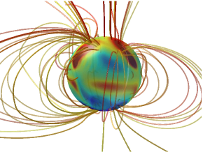
(a)

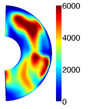
(b)

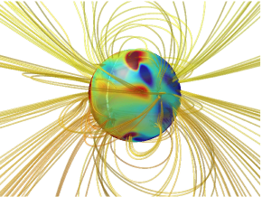
(c)

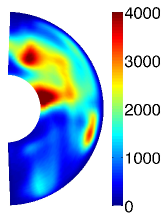
(d)

Figure 1: (a): radial magnetic field $B_{r}$ at the core-mantle boundary for the axial dipolar solution $D$. Magnetic field lines are also shown. (b): total magnetic energy (azimuthally averaged) in the meridional plane. The solution $D$ corresponds to a strong dipolar magnetic field, with a distribution of the magnetic energy relatively symmetrical, although slightly larger in the northern hemisphere. (b) and (c): same thing, but showing the equatorial dipolar solution $E$ observed at larger values of $C$. The solution $E$ takes the form of an equatorial dipole at the outer surface, but the total magnetic field in the bulk of the flow is strongly hemispherical.

Fig. 1a and 1b show the solution obtained for $C=0.1$, when the symmetry breaking is relatively weak. For this value, the magnetic field is strongly dominated by its axisymmetric component and the radial magnetic field measured at the core-mantle boundary shows a strong dipolar component (Fig. 1a). A weaker non-axisymmetric component, reminiscent from the $m=3$ convection pattern, is also visible. This magnetic structure is quite similar to the one obtained in the absence of symmetry breaking. Fig. 1b represents the total magnetic energy averaged in the $\phi$-direction, shown in the poloidal plane ($r,\theta$). Despite the heterogeneous temperature gradient, the magnetic energy remains largely symmetrical with respect to the equator.

For larger symmetry breaking, this dipole is replaced by a totally different solution, hereafter referred as solution $E$. Fig. 1c and 1d show the magnetic structure obtained for $C=0.2$. The magnetic field is now dominated by a non-axisymmetric $m=1$ component. At the outer sphere, the field corresponds to an equatorial dipole, rotating around the $z$-axis and slightly stronger in the northern hemisphere. In the bulk of the flow, the equatorial asymmetry of the field becomes more important, as shown by the magnetic energy distribution (Fig. 1d), and this new solution therefore takes the form of an hemispherical magnetic field (a similar behavior was reported in Stanley08 ). Although the thermal convection is made more vigorous in the southern hemisphere by the heterogeneous heating, note that the magnetic energy is surprisingly localized in the northern hemisphere.

The generation of an equatorial dipole has been reported in previous numerical studies. An equatorial dipole solution was described for Rayleigh number very close to the onset of convection Ishihara02 , and a similar solution was found in Aubert04 for smaller shell thickness. In our case, the breaking of the equatorial symmetry is directly responsible for the generation of the equatorial dipole. For the range of $C$ studied here, the total kinetic energy remains relatively symmetrical with respect to the equatorial plane (for $C=0.1$, the equatorially antisymmetric flow energy is only $10\%$ of the symmetrical one). However, this weak symmetry breaking is sufficient to strongly modify the axisymmetric velocity, by generating a large counter-rotating zonal flow. This toroidal $t_{2}^{0}$ flow introduces a strong shear in the equatorial plane which tends to favor the equatorial dipole at the expense of the axial one.

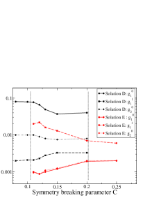
Figure 2: Bifurcation of the coefficients $g_{1}^{0}$, $g_{1}^{1}$ and $g_{2}^{0}$ of the magnetic energy as a function of the symmetry breaking parameter $C$. For $0.1<C<0.2$, there is a bistability between the axial dipole solution $D$ (black) and the equatorial dipole solution $E$ (red). Turbulent fluctuations connect the two solutions.

An interesting behavior occurs for intermediate values of the symmetry breaking. When $0.1<C<0.2$, a bistability between the axial dipole $D$ and the non-axisymmetric solution $E$ is indeed obtained. Fig. 2 illustrates this bistable regime by showing the bifurcation of both modes as a function of $C$. The axial dipolar solution $D$ is shown in black, and the solution $E$ dominated by $m=1$ magnetic modes in red. For each of these solutions, we show the coefficients of the axial dipole $g_{1}^{0}$, the equatorial dipole $g_{1}^{1}$, and the axial quadrupole $g_{2}^{0}$, where $g_{l}^{m}$ means the poloidal component of the spherical harmonic of order $l$ and degree $m$. The dashed vertical lines in Fig. 2 indicate the region for which the system is bistable: both solutions can be obtained depending on the initial conditions of the simulation. Note that for the solution $E$, dipolar and quadrupolar components possess the same amplitude, in agreement with the hemispherical structure of the magnetic field.

More interestingly, when the magnetic field is in this bistable regime, for $0.1<C<0.2$, the strong fluctuations generated by the turbulence of the flow allow the system to switch from one solution to the other. These transitions between the axial and the equatorial dipole are shown by the time series of the energy of the system in Fig. 3-left: the two states, although strongly fluctuating, are clearly distinguishable by different well defined mean values for the energies of axial (black) and equatorial (red) dipoles, and the system randomly switch from one state to the other. In addition, Fig. 3-right shows the time evolution of the $g_{1}^{0}$ and the $g_{1}^{1}$ at the core-mantle boundary. Since the phase space is symmetrical with respect to the symmetry $D\rightarrow-D$, we observe transitions from $E$ to $D$ as well as transitions from $E$ to $-D$. This bistability between the axial dipole and the equatorial one therefore takes the form of chaotic reversals of the polarity of the axial dipole. During a reversal, the dipolar magnetic field does not vanish, but rather tilts at $90^{o}$ and rotates in the equatorial plane.

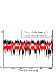
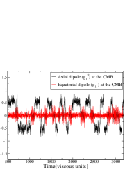
Figure 3: Time evolution of the magnetic field for $C=0.13$. The system chaotically jumps between the bistable solutions $E$ and $\pm D$. Left: Magnetic energy of the equatorial (red) and axial (black) dipoles. Right : Same thing, but at the core-mantle boundary. The bistability with the equatorial dipole yields chaotic polarity reversals of the axial dipolar magnetic field.

In Fig. 3, the dipolar magnetic field spends approximatively as much time aligned with the axis of rotation (solution $D$) as tilted at $90^{o}$ (solution $E$). In fact, the total time spent in one state or the other strongly depends on the amplitude of the symmetry breaking. Fig. 4 shows the probability density function of the dipolar component $g_{1}^{0}$ for different values of $C$. For $C\leq 0.1$ (black curve), the equatorial dipole $E$ is not excited, and only the dipolar configuration $D$ is accessible: the field does not reverse, and the probability picks around $D$ or $-D$, depending on the initial conditions. When $C$ is slightly increased, the system starts to briefly explore the equatorial dipolar state, in addition to $D$. The PDF is thus characterized by a non-zero value at $g_{1}^{0}=0$, corresponding to the solution $E$. By symmetry, this solution is identically connected to $D$ or $-D$, allowing the axial dipole to reverse the sign of its polarity. For $0.1<C<0.2$, the probability density function of the axial dipole is then trimodal. Finally, when $C$ is sufficiently large, only the equatorial dipole solution $E$ remains, and the probability of $g_{1}^{0}$ is centered around zero.

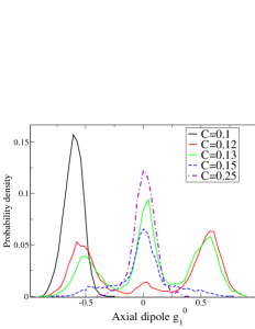
Figure 4: Probability density function of the axial dipolar component at the core-mantle boundary, for different values of $C$. Depending on the value of $C$, the distribution can be picked around a non-zero value of $g_{1}^{0}$ (small $C$, solution $D$) or around zero (large $C$, solution $E$). In the bistable regime, the distribution can be bimodal or trimodal.

During this transition from a non-reversing dipolar magnetic field to an oscillating $m=1$ mode, one can also study the direction of the dipole (Fig. 5). The black curve shows the probability $P_{D}$ of finding the system in the axial configuration (more precisely, $P_{D}$ is defined as the probability that $\sin(\theta_{D})<0.25$, where $\theta_{D}$ is the dipole tilt angle). The transition is very sharp, the axial dipole probability dropping abruptly from one to zero for $C>0.1$. On the contrary, the probability of finding the equatorial dipole ($\sin(\theta_{D})>0.75$) rapidly increases from zero to one when $C$ is increased. The red curve shows the reversal frequency of the dipolar solution $D$ versus the symmetry breaking $C$. When $C$ is increased, the connection with the attractor $E$ corresponding to the equatorial solution is larger. Consequently, the connections between the two opposite states $D$ and $-D$ are more frequent, and the number of reversals increases.

For $C\sim 0.1$, at the very beginning of this transition, the system spends a long time in the solution $D$. It still explores the equatorial configuration, but only for a very brief moment during reversals or excursions. In this case, the distribution tends to be bimodal (red curve, Fig. 4), despite the fact that three stable states are involved in the reversal. For instance, the inset of Fig. 5 shows the time evolution of the dipole tilt for $C=0.12$ and illustrates how a weak equatorial symmetry breaking can produce ’Earth-like’ reversals, with a bimodal distribution and a dipole tilt rapidly switching from $0^{o}$ to $180^{o}$.

It is possible to give a naive picture of this mechanism using the analogy with a heavily damped particle in a tristable potential (a different but close mechanism is described in Hoyng01 by picturing the geodynamo as a bistable oscillator): most of the time, the system is trapped inside one of the wells (corresponding to $D$ or $-D$). Due to turbulent fluctuations, the system eventually escapes one of these stable minima to reaches the opposite one. Between these two opposite states, there is a third stable potential well, the equatorial dipole $E$, which creates a connection between $D$ and $-D$. As $C$ is increased, an exchange of stability takes place from the potential wells $\pm D$ toward $E$, and reversals become more frequent (for $C>0.2$, when only $E$ persists, the axial dipole simply fluctuates around zero). Simply stated, reversals of the axial dipolar field thus rely on the presence of the equatorial dipole, which is used as a transitional field during each reversal.

Interestingly, this scenario shares strong similarities with the mechanism for reversals observed in classical geodynamo simulations: when an homogeneous heat flux is used, reversals of the dipole field are only observed within a particular transition region of the parameter space, between a regime in which the field is strongly dipolar and a regime strongly fluctuating characterized by a multipolar magnetic structure Olson06 , Schrinner10 . In this case, reversals also result from a bistability between the dipole and another mode (the multipolar mode), similarly to what happens here with the equatorial dipole. As in our case, ’Earth-like’ reversals are obtained only if the system is chosen inside the transition region, but only at the very beginning of this transition, close to the boundary with the dipolar regime.

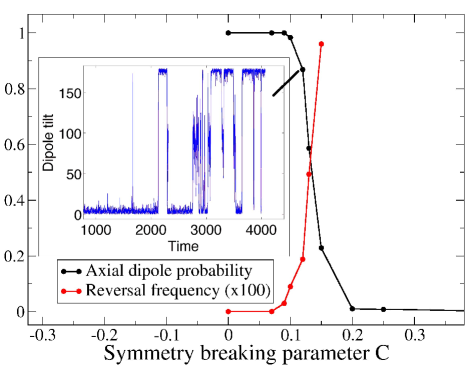
Figure 5: Black: probability for finding the axial dipolar solution, as a function of $C$. The transition from an axial to an equatorial dipole field is very sharp. Red: Reversal frequency of the axial dipole. As $C$ increases, the basin of attraction of the equatorial dipole extends, allowing for more and more reversals of the axial dipole. Inset: Time evolution of the dipole tilt $\theta_{D}$ for $C=0.12$: the system spends a very weak portion of time in the non-axisymmetric state, and ’Earth-like’ reversals can be obtained.

Although based on a different mechanism, the behavior of the magnetic field also has interesting similarities with the model proposed in Petrelis09 : reversals are triggered by the equatorial symmetry breaking, and result from the interaction between the so-called dipole and quadrupole families of the magnetic field. The intriguing generation of a strongly hemispherical solution at very small symmetry breaking is also predicted by this model Gallet09 . In fact, depending on the parameters, this model can lead to an hemispherical solution like the one reported here, or yields polarity reversals through a saddle-node bifurcation. However, numerical simulations have shown that this later mechanism is rather selected at sufficiently small $Pm$ Gissinger10 , whereas the simulations reported here are carried at $Pm=20$. Although small $Pm$ simulations are numerically challenging, it would be interesting to study how the mechanism described in this letter is modified as $Pm$ is decreased towards more realistic values.

To summarize, we have shown that an equatorial dipole solution can be generated in geodynamo simulations when the equatorial symmetry of the flow is broken by an heterogeneous heating at the core-mantle boundary. Moreover, for weak symmetry breaking, a bistable regime between this equatorial dipole and the axial dipole is obtained. Finally, this bistability leads to an interesting scenario for geomagnetic reversals: The symmetry breaking, by stabilizing the equatorial dipole, provides the system with a new solution for connecting the two axial dipole polarities, and sufficiently strong turbulent fluctuations trigger chaotic reversals of the field. During a reversal, the transitional field is strongly hemispherical in the bulk of the flow, and corresponds to an equatorial dipole field at the core-mantle boundary, rotating around the $z$-axis. In agreement with paleomagnetic observations, the reversal frequency is directly related to the equatorial asymmetry of the flow.