A Novel Robust Approach to Least Squares Problems with Bounded Data Uncertainties

Nargiz Kalantarova, Mehmet A. Donmez, and Suleyman S. Kozat, Senior Member, IEEE Suleyman S. Kozat, Nargiz Kalantarova, and Mehmet A. Donmez (skozat, nkalantarova, medonmez@ku.edu.tr) are with the EE Department at the Koc University, Istanbul, tel:+902123381000.
Abstract

In this correspondence, we introduce a minimax regret criteria to the least squares problems with bounded data uncertainties and solve it using semi-definite programming. We investigate a robust minimax least squares approach that minimizes a worst case difference regret. The regret is defined as the difference between a squared data error and the smallest attainable squared data error of a least squares estimator. We then propose a robust regularized least squares approach to the regularized least squares problem under data uncertainties by using a similar framework. We show that both unstructured and structured robust least squares problems and robust regularized least squares problem can be put in certain semi-definite programming forms. Through several simulations, we demonstrate the merits of the proposed algorithms with respect to the the well-known alternatives in the literature.

Index Terms:
Least squares, deterministic, regret, regularization, minimax.

EDICS Category: SPC-DETC

I Introduction

We study estimation of a deterministic signal observed through an unknown deterministic data matrix under additive noise [1]. Although the observation matrix and the output vector are not exactly known, estimates for both the data matrix and the output vector, as well as uncertainty bounds on them, are given [2, 3]. When there are uncertainties in the model parameters, a common approach to estimate the input signal is to use the robust least squares (LS) method [1], since the classical LS estimators perform poorly when the perturbations on the model parameters are relatively high [1, 3, 2]. Although the robust LS methods are able to minimize the data error for the worst case perturbations, however, they usually provide unsatisfactory results on the average [2]. Therefore, in order to counterbalance the conservative nature of the robust LS methods [1], we introduce a novel robust LS approach that minimizes a worst case “regret” that is defined as the difference between the squared data error and the smallest attainable squared data error with an LS estimator. By this regret formulation, we seek a linear estimator whose performance is as close as possible to that of the optimal estimator for all possible perturbations on the data matrix and the output vector. Our main goal in proposing the minimax regret formulation is to provide a trade-off between the robust LS methods tuned to the worst possible model parameters (under the uncertainty bounds) and the optimal LS estimator tuned to the underlying unknown model parameters. Furthermore, after studying the data estimation problems in the presence of bounded data uncertainties, we extend the regret formulation to the regularized LS problem, where the regret is defined as the difference between the cost of the regularized LS algorithm [4, 3], and the smallest attainable cost with a linear regularized LS estimator. Under these frameworks, we provide the solutions for the proposed regret based minimax LS and the regret based minimax regularized LS approaches in semi-definite programming (SDP) forms. We emphasize that SDP problems can be efficiently solved even for real-time applications [5].

A wide range of applications in the signal processing literature deal with LS problems [3, 2, 6, 1]. However, in different applications, the performance of the LS estimators may substantially degrade due to possible errors in the model parameters. One of the conventional approaches to find robust solutions to such estimation problems is the robust LS method [1, 3], in which the uncertainties in the data matrix and the output vector are incorporated in optimization via a minimax residual formulation. Another approach to compensate for data errors is the total least squares method [2], which may be undesirable since it may yield conservative results due to data de-regularization. Furthermore, in many linear regression problems, the data matrix has a known special structure, e.g., Toeplitz [1, 2]. The performance of the minimax methods usually improve when such a prior knowledge is integrated in the problem formulation [1, 2].

In order to mitigate the pessimistic nature of the worst case optimization methods, the minimax regret approaches have been introduced in the context of statistical signal processing literature [7, 8, 9, 10]. However, we emphasize that the robust methods studied in this correspondence substantially differ from [1, 3, 7, 8, 10]. The cost functions studied here are different than [1, 3], where the regret terms are directly appended in the cost functions. Although in [7, 8, 10] a similar regret notion is used, the cost function as well as the constraints are substantially different in this correspondence. Furthermore, note that in [7], the uncertainty is in the statistics of the transmitted signal. On the other hand, in [8] and [10], the uncertainty is in the transmitted signal and the channel parameters, respectively, unlike in here. In this correspondence, the uncertainty is both on the data matrix and the output vector. Furthermore, since the cost functions are different for our formulations, the solutions to the LS problems presented in this correspondence cannot be obtained from [7, 8, 10]. We emphasize that the proposed methods are formulated for given perturbation bounds and note that such bounds heavily depend on the estimation algorithms used to obtain the observation matrix and the data matrix. In this sense, different estimation algorithms can be readily incorporated in our framework with the corresponding uncertainty bounds [3].

Our main contributions are as follows. We first introduce a novel LS approach in which we seek to find the transmitted data by minimizing the worst case difference between the data error of the LS estimator and the data error with the optimal LS estimator. With this method, we aim to provide a trade off between the performance of the robust LS methods and the tuned LS estimator (tuned to the unknown data matrix and the output vector). Then, we develop a minimax regret approach for the regularized LS problem. We demonstrate that the proposed robust methods can be cast as SDP problems. In our simulations, we observe that the proposed approaches yield better performance compared to the robust methods optimized with respect to the worst case data error [1, 3], and the tuned LS and the tuned regularized LS estimators (tuned to the estimated data matrix and the output vector), respectively.

The organization of the correspondence is as follows. We initially provide an overview of the problem in Section II. In Section III, we introduce the unstructured and regularized LS approaches based on the regret formulation. We then continue to study the structured LS approach. The numerical examples are given in Section IV. Finally, the correspondence concludes with some remarks in Section V.

II System Overview

We consider the problem of estimating a deterministic vector $\mbox{$\mbox{$\mathbf{u}$}$}\in\mathbb{R}^{n}$ which is observed through a deterministic data matrix. However, instead of the actual coefficient matrix and the output vector, their estimates $\mbox{$\mbox{$\mathbf{H}$}$}\in\mathbb{R}^{m\times n}$ and $\mbox{$\mbox{$\mathbf{y}$}$}\in\mathbb{R}^{m}$ and uncertainty bounds on the estimates are provided, where $m\geq n$111All vectors are column vectors and denoted by boldface lowercase letters. Matrices are represented by boldface uppercase letters. For a vector $\mathbf{u}$, $\|\mbox{$\mbox{$\mathbf{u}$}$}\|=\sqrt{\mbox{$\mbox{$\mathbf{u}$}$}^{T}\mbox{$\mbox{$\mathbf{u}$}$}}$ is the $\ell_{2}$-norm, where $\mbox{$\mbox{$\mathbf{u}$}$}^{T}$ is the ordinary transpose. For a matrix $\mathbf{H}$, $\lVert\mbox{$\mbox{$\mathbf{H}$}$}\rVert$ implies the Frobenius norm. For a vector $\mathbf{u}$, $\mathrm{diag}(\mbox{$\mbox{$\mathbf{u}$}$})$ is a diagonal matrix constructed from the entries of $\mathbf{u}$. For a square matrix $\mathbf{H}$, $\mathrm{Tr}(\mbox{$\mathbf{H}$})$ is the trace. $\mathbf{0}$ denotes a vector or matrix with all zero elements and the dimension can be understood from the context. The operator $\mathrm{vec}(\cdot)$ stacks the columns of a matrix of dimension $m\times n$ into a $mn\times 1$ column vector, and the operator $\otimes$ is the Kronecker product [11].. Our goal is to find a solution to the data estimation problem $\mbox{$\mbox{$\mathbf{H}$}$}\mbox{$\mbox{$\mathbf{u}$}$}\approx\mbox{$\mbox{$\mathbf{y}$}$}$, such that $(\mbox{$\mbox{$\mathbf{H}$}$}+\Delta\mbox{$\mathbf{H}$})\mbox{$\mbox{$\mathbf{u}$}$}=\mbox{$\mbox{$\mathbf{y}$}$}+\Delta\mbox{$\mathbf{y}$}$ for deterministic perturbations $\Delta\mbox{$\mathbf{H}$}\in\mathbb{R}^{m\times n}$, $\Delta\mbox{$\mathbf{y}$}\in\mathbb{R}^{m}$, which are unknown but a bound on each of the perturbation is provided, i.e., $\lVert\Delta\mbox{$\mathbf{H}$}\rVert\leq\mbox{$\delta$}_{H}$ and $\lVert\Delta\mbox{$\mathbf{y}$}\rVert\leq\mbox{$\delta$}_{Y}$, where $\mbox{$\delta$}_{H},\mbox{$\delta$}_{Y}\geq 0$.

Even under the uncertainties, the unknown vector $\mathbf{u}$ can be naively estimated by simply substituting the estimates $\mathbf{H}$ and $\mathbf{y}$ into the LS estimator [4]. For the LS estimator we have $\hat{\mbox{$\mbox{$\mathbf{u}$}$}}=\mbox{$\mbox{$\mathbf{H}$}$}^{+}\mbox{$\mbox{$\mathbf{y}$}$}$, where $\mbox{$\mbox{$\mathbf{H}$}$}^{+}$ is the pseudo-inverse of $\mathbf{H}$ [11]. However, this approach does not yield acceptable results, when the errors in the estimates are relatively high [1, 7, 8]. A common approach to find a robust solution is to use a worst case residual optimization [1] as

$$\hat{\mbox{$\mbox{$\mathbf{u}$}$}}=\mathrm{arg}\min_{\mbox{$\mbox{$\mathbf{u}$}$}}\max_{\lVert\Delta\mbox{$\mathbf{H}$}\rVert\leq\mbox{$\delta$}_{H},\lVert\Delta\mbox{$\mathbf{y}$}\rVert\leq\mbox{$\delta$}_{Y},}{\lVert(\mbox{$\mbox{$\mathbf{H}$}$}+\Delta\mbox{$\mathbf{H}$})\mbox{$\mbox{$\mathbf{u}$}$}-(\mbox{$\mbox{$\mathbf{y}$}$}+\Delta\mbox{$\mathbf{y}$})\rVert}^{2},$$

where $\mathbf{u}$ is found by minimizing the worst case error in the uncertainty region. However, the solution may be highly conservative, since the solution is found with respect to the worst possible coefficient matrix and output vector in the uncertainty regions [2, 7, 8]. In order to alleviate the conservative nature of the worst case residual approach as well as to preserve robustness, we propose a novel LS approach, which provides a trade off between performance and robustness [7, 8]. The regret for not using the optimal LS estimator is defined as the difference between the squared data error with an estimate of the input vector and the squared data error with the optimal LS estimator

$${\cal R}(\Delta\mbox{$\mathbf{H}$},\Delta\mbox{$\mathbf{y}$})\stackrel{{\scriptstyle\bigtriangleup}}{{=}}{\lVert(\mbox{$\mbox{$\mathbf{H}$}$}+\Delta\mbox{$\mathbf{H}$})\mbox{$\mbox{$\mathbf{u}$}$}-(\mbox{$\mbox{$\mathbf{y}$}$}+\Delta\mbox{$\mathbf{y}$})\rVert}^{2}-\min_{\mbox{$\mbox{$\mathbf{w}$}$}}{\lVert(\mbox{$\mbox{$\mathbf{H}$}$}+\Delta\mbox{$\mathbf{H}$})\mbox{$\mbox{$\mathbf{w}$}$}-(\mbox{$\mbox{$\mathbf{y}$}$}+\Delta\mbox{$\mathbf{y}$})\rVert}^{2},$$

where $\lVert\Delta\mbox{$\mathbf{H}$}\rVert\leq\mbox{$\delta$}_{H}$, $\lVert\Delta\mbox{$\mathbf{y}$}\rVert\leq\mbox{$\delta$}_{Y}$, for some $\mbox{$\delta$}_{H},\mbox{$\delta$}_{Y}\geq 0$. In the next section, the proposed approaches to the LS problems are provided. First, the regret based unstructured LS method is introduced. Then, the unstructured regularized LS approach is presented in which the worst case regret is optimized, where the regret is defined as the difference between the cost function of the regularized LS algorithm [4] with an input vector and the cost function with the optimal regularized LS estimator. Finally, the structured LS approach is studied.

III Robust Least Squares Methods

III-A Unstructured Robust Least Squares

In this section, we develop a novel unstructured LS estimator based on a certain minimax criteria. Let $\mbox{$\mbox{$\mathbf{H}$}$}\in\mathbb{R}^{m\times n}$, $\mbox{$\mbox{$\mathbf{y}$}$}\in\mathbb{R}^{m}$, $m\geq n$, and $\mbox{$\delta$}_{H},\mbox{$\delta$}_{Y}\geq 0$. We find $\mathbf{u}$ that is the solution to the following optimization problem:

$$\min_{\mbox{$\mbox{$\mathbf{u}$}$}}\max_{\lVert\Delta\mbox{$\mathbf{H}$}\rVert\leq\mbox{$\delta$}_{H},\lVert\Delta\mbox{$\mathbf{y}$}\rVert\leq\mbox{$\delta$}_{Y}}\big{\{}{\lVert(\mbox{$\mbox{$\mathbf{H}$}$}+\Delta\mbox{$\mathbf{H}$})\mbox{$\mbox{$\mathbf{u}$}$}-(\mbox{$\mbox{$\mathbf{y}$}$}+\Delta\mbox{$\mathbf{y}$})\rVert}^{2}-\min_{\mbox{$\mbox{$\mathbf{w}$}$}}{\lVert(\mbox{$\mbox{$\mathbf{H}$}$}+\Delta\mbox{$\mathbf{H}$})\mbox{$\mbox{$\mathbf{w}$}$}-(\mbox{$\mbox{$\mathbf{y}$}$}+\Delta\mbox{$\mathbf{y}$})\rVert}^{2}\big{\}}.$$ (1)

Note that by unconstraint minimization over $\mathbf{w}$, we have $g(\mbox{$\tilde{\mbox{$\mathbf{H}$}}$},\mbox{$\tilde{\mbox{$\mathbf{y}$}}$})\stackrel{{\scriptstyle\bigtriangleup}}{{=}}\lVert(\mbox{$\mathbf{I}$}-\mbox{$\tilde{\mbox{$\mathbf{H}$}}$}\mbox{$\tilde{\mbox{$\mathbf{H}$}}$}^{+})\mbox{$\tilde{\mbox{$\mathbf{y}$}}$}\rVert^{2}=\min_{\mbox{$\mbox{$\mathbf{w}$}$}}{\lVert(\mbox{$\mbox{$\mathbf{H}$}$}+\Delta\mbox{$\mathbf{H}$})\mbox{$\mbox{$\mathbf{w}$}$}-(\mbox{$\mbox{$\mathbf{y}$}$}+\Delta\mbox{$\mathbf{y}$})\rVert}^{2}$, $\mbox{$\tilde{\mbox{$\mathbf{H}$}}$}\stackrel{{\scriptstyle\bigtriangleup}}{{=}}\mbox{$\mbox{$\mathbf{H}$}$}+\Delta\mbox{$\mathbf{H}$}$, $\mbox{$\tilde{\mbox{$\mathbf{y}$}}$}\stackrel{{\scriptstyle\bigtriangleup}}{{=}}\mbox{$\mbox{$\mathbf{y}$}$}+\Delta\mbox{$\mathbf{y}$}$. If we use the first order Taylor series expansion [11] for $g(\mbox{$\tilde{\mbox{$\mathbf{H}$}}$},\mbox{$\tilde{\mbox{$\mathbf{y}$}}$})$, then

$\displaystyle g(\mbox{$\tilde{\mbox{$\mathbf{H}$}}$},\mbox{$\tilde{\mbox{$\mathbf{y}$}}$})=g(\mbox{$\mbox{$\mathbf{H}$}$},\mbox{$\mbox{$\mathbf{y}$}$})+2\mathrm{Tr}\bigg{\{}\nabla g(\mbox{$\tilde{\mbox{$\mathbf{H}$}}$},\mbox{$\tilde{\mbox{$\mathbf{y}$}}$})|_{\mbox{$\tilde{\mbox{$\mathbf{H}$}}$}=\mbox{$\mbox{$\mathbf{H}$}$},\mbox{$\tilde{\mbox{$\mathbf{y}$}}$}=\mbox{$\mbox{$\mathbf{y}$}$}}^{T}\big{[}\Delta\mbox{$\mathbf{H}$}\hskip 7.22743pt\Delta\mbox{$\mathbf{y}$}\big{]}\bigg{\}}+O\big{(}\lVert\big{[}\Delta\mbox{$\mathbf{H}$}\hskip 7.22743pt\Delta\mbox{$\mathbf{y}$}\big{]}\rVert^{2}\big{)}.$ (2)

Clearly, the effect of this approximation vanishes as $\lVert\big{[}\Delta\mbox{$\mathbf{H}$}\hskip 7.22743pt\Delta\mbox{$\mathbf{y}$}\big{]}\rVert$ decreases, however, we observe through our simulations that even for relatively large perturbations a satisfactory performance is obtained. Since $\dfrac{\partial g(\mbox{$\tilde{\mbox{$\mathbf{H}$}}$},\mbox{$\tilde{\mbox{$\mathbf{y}$}}$})}{\partial\mbox{$\tilde{\mbox{$\mathbf{y}$}}$}}|_{\mbox{$\tilde{\mbox{$\mathbf{H}$}}$}=\mbox{$\mbox{$\mathbf{H}$}$},\mbox{$\tilde{\mbox{$\mathbf{y}$}}$}=\mbox{$\mbox{$\mathbf{y}$}$}}=2(\mbox{$\mathbf{I}$}-\mbox{$\mbox{$\mathbf{H}$}$}\mbox{$\mbox{$\mathbf{H}$}$}^{+})\mbox{$\mbox{$\mathbf{y}$}$}$ and based on the approximation (2), the regret in (1) can be written as

$\displaystyle{\cal R}(\Delta\mbox{$\mathbf{H}$},\Delta\mbox{$\mathbf{y}$})$ $\displaystyle\approx{\lVert(\mbox{$\mbox{$\mathbf{H}$}$}+\Delta\mbox{$\mathbf{H}$})\mbox{$\mbox{$\mathbf{u}$}$}-(\mbox{$\mbox{$\mathbf{y}$}$}+\Delta\mbox{$\mathbf{y}$})\rVert}^{2}-g(\mbox{$\mbox{$\mathbf{H}$}$},\mbox{$\mbox{$\mathbf{y}$}$})-2\mathrm{Tr}\bigg{\{}\nabla g(\mbox{$\tilde{\mbox{$\mathbf{H}$}}$},\mbox{$\tilde{\mbox{$\mathbf{y}$}}$})|_{\mbox{$\tilde{\mbox{$\mathbf{H}$}}$}=\mbox{$\mbox{$\mathbf{H}$}$},\mbox{$\tilde{\mbox{$\mathbf{y}$}}$}=\mbox{$\mbox{$\mathbf{y}$}$}}^{T}\big{[}\Delta\mbox{$\mathbf{H}$}\hskip 7.22743pt\Delta\mbox{$\mathbf{y}$}\big{]}\bigg{\}}$
$\displaystyle={\lVert(\mbox{$\mbox{$\mathbf{H}$}$}+\Delta\mbox{$\mathbf{H}$})\mbox{$\mbox{$\mathbf{u}$}$}-(\mbox{$\mbox{$\mathbf{y}$}$}+\Delta\mbox{$\mathbf{y}$})\rVert}^{2}-\mbox{$\xi$}-2\big{(}\mathrm{vec}(\mbox{$\mathbf{D}$})^{T}\mathrm{vec}(\Delta\mbox{$\mathbf{H}$})+2\Delta\mbox{$\mathbf{y}$}^{T}\mbox{$\mathbf{P}$}^{\perp}_{\mbox{$\mbox{$\mathbf{H}$}$}}\mbox{$\mbox{$\mathbf{y}$}$}+2\mbox{$\mbox{$\mathbf{y}$}$}^{T}\mbox{$\mathbf{P}$}^{\perp}_{\mbox{$\mbox{$\mathbf{H}$}$}}\Delta\mbox{$\mathbf{y}$}\big{)}$
$\displaystyle={\lVert(\mbox{$\mbox{$\mathbf{H}$}$}+\Delta\mbox{$\mathbf{H}$})\mbox{$\mbox{$\mathbf{u}$}$}-(\mbox{$\mbox{$\mathbf{y}$}$}+\Delta\mbox{$\mathbf{y}$})\rVert}^{2}-\big{(}\mbox{$\xi$}+\mbox{$\mathbf{c}$}^{T}\mbox{$\mathbf{h}$}+\mbox{$\mathbf{h}$}^{T}\mbox{$\mathbf{c}$}+\Delta\mbox{$\mathbf{y}$}^{T}\mbox{$\mathbf{b}$}+\mbox{$\mathbf{b}$}^{T}\Delta\mbox{$\mathbf{y}$}\big{)},$ (3)

where $\mbox{$\mathbf{D}$}\stackrel{{\scriptstyle\bigtriangleup}}{{=}}\dfrac{\partial g(\mbox{$\tilde{\mbox{$\mathbf{H}$}}$},\mbox{$\tilde{\mbox{$\mathbf{y}$}}$})}{\partial\mbox{$\tilde{\mbox{$\mathbf{H}$}}$}}|_{\mbox{$\tilde{\mbox{$\mathbf{H}$}}$}=\mbox{$\mbox{$\mathbf{H}$}$},\mbox{$\tilde{\mbox{$\mathbf{y}$}}$}=\mbox{$\mbox{$\mathbf{y}$}$}}$, $\mbox{$\mathbf{P}$}^{\perp}_{\mbox{$\mbox{$\mathbf{H}$}$}}\stackrel{{\scriptstyle\bigtriangleup}}{{=}}(\mbox{$\mathbf{I}$}-\mbox{$\mbox{$\mathbf{H}$}$}\mbox{$\mbox{$\mathbf{H}$}$}^{+})$ is the projection matrix of the space perpendicular to the range space of $\mathbf{H}$, $\mbox{$\xi$}\stackrel{{\scriptstyle\bigtriangleup}}{{=}}f(\mbox{$\mbox{$\mathbf{H}$}$},\mbox{$\mbox{$\mathbf{y}$}$})$, $\mbox{$\mathbf{h}$}\stackrel{{\scriptstyle\bigtriangleup}}{{=}}\mathrm{vec}(\Delta\mbox{$\mathbf{H}$})$, $\mbox{$\mathbf{c}$}\stackrel{{\scriptstyle\bigtriangleup}}{{=}}\mathrm{vec}(\mbox{$\mathbf{D}$})$ and $\mbox{$\mathbf{b}$}\stackrel{{\scriptstyle\bigtriangleup}}{{=}}2\mbox{$\mathbf{P}$}^{\perp}_{\mbox{$\mbox{$\mathbf{H}$}$}}\mbox{$\mbox{$\mathbf{y}$}$}$.

In the following theorem, we illustrate how the problem of minimization of the worst case regret (3) can be put in an SDP form.
Theorem 1: Let $\mbox{$\mbox{$\mathbf{H}$}$}\in\mathbb{R}^{m\times n}$, $\mbox{$\mbox{$\mathbf{y}$}$}\in\mathbb{R}^{m}$, $m\geq n$, and $\mbox{$\delta$}_{H},\mbox{$\delta$}_{Y}\geq 0$, then

$$\min_{\mbox{$\mbox{$\mathbf{u}$}$}}\max_{\lVert\Delta\mbox{$\mathbf{H}$}\rVert\leq\mbox{$\delta$}_{H},\lVert\Delta\mbox{$\mathbf{y}$}\rVert\leq\mbox{$\delta$}_{Y}}\bigg{\{}{\lVert(\mbox{$\mbox{$\mathbf{H}$}$}+\Delta\mbox{$\mathbf{H}$})\mbox{$\mbox{$\mathbf{u}$}$}-(\mbox{$\mbox{$\mathbf{y}$}$}+\Delta\mbox{$\mathbf{y}$})\rVert}^{2}-f(\mbox{$\mbox{$\mathbf{H}$}$},\mbox{$\mbox{$\mathbf{y}$}$})-2\mathrm{Tr}\big{\{}\nabla g(\mbox{$\tilde{\mbox{$\mathbf{H}$}}$},\mbox{$\tilde{\mbox{$\mathbf{y}$}}$})|_{\mbox{$\tilde{\mbox{$\mathbf{H}$}}$}=\mbox{$\mbox{$\mathbf{H}$}$},\mbox{$\tilde{\mbox{$\mathbf{y}$}}$}=\mbox{$\mbox{$\mathbf{y}$}$}}^{T}\big{[}\Delta\mbox{$\mathbf{H}$}\hskip 7.22743pt\Delta\mbox{$\mathbf{y}$}\big{]}\big{\}}\bigg{\}}$$ (4)

is equivalent to solving the following SDP problem

$$\min\mbox{$\gamma$}\mbox{ subject to}$$
$$\left[\begin{array}[]{cccc}\mbox{$\gamma$}+\mbox{$\xi$}-\tau-\theta&\left(\mbox{$\mbox{$\mathbf{H}$}$}\mbox{$\mbox{$\mathbf{u}$}$}-\mbox{$\mbox{$\mathbf{y}$}$}\right)^{T}&\mbox{$\delta$}_{H}\mbox{$\mathbf{c}$}^{T}&\mbox{$\delta$}_{Y}\mbox{$\mathbf{b}$}^{T}\\ \left(\mbox{$\mbox{$\mathbf{H}$}$}\mbox{$\mbox{$\mathbf{u}$}$}-\mbox{$\mbox{$\mathbf{y}$}$}\right)&\mbox{$\mathbf{I}$}&\mbox{$\delta$}_{H}\mbox{$\mathbf{U}$}&-\mbox{$\delta$}_{Y}\mbox{$\mathbf{I}$}\\ \mbox{$\delta$}_{H}\mbox{$\mathbf{c}$}&\mbox{$\delta$}_{H}\mbox{$\mathbf{U}$}^{T}&\tau\mbox{$\mathbf{I}$}&\mbox{$\mathbf{0}$}\\ \mbox{$\delta$}_{Y}\mbox{$\mathbf{b}$}&-\mbox{$\delta$}_{Y}\mbox{$\mathbf{I}$}&\mbox{$\mathbf{0}$}&\theta\mbox{$\mathbf{I}$}\end{array}\right]\geq 0,$$ (5)

where $g(\mbox{$\tilde{\mbox{$\mathbf{H}$}}$},\mbox{$\tilde{\mbox{$\mathbf{y}$}}$})=\mbox{$\tilde{\mbox{$\mathbf{y}$}}$}^{T}(\mbox{$\mathbf{I}$}-\mbox{$\tilde{\mbox{$\mathbf{H}$}}$}\mbox{$\tilde{\mbox{$\mathbf{H}$}}$}^{+})\mbox{$\tilde{\mbox{$\mathbf{y}$}}$}$, $\mbox{$\xi$}=\mbox{$\mbox{$\mathbf{y}$}$}^{T}(\mbox{$\mathbf{I}$}-\mbox{$\mbox{$\mathbf{H}$}$}\mbox{$\mbox{$\mathbf{H}$}$}^{+})\mbox{$\mbox{$\mathbf{y}$}$}$, $\tau,\theta\geq 0$, $\mbox{$\mathbf{c}$}=\mathrm{vec}\left(\dfrac{\partial g(\mbox{$\tilde{\mbox{$\mathbf{H}$}}$},\mbox{$\tilde{\mbox{$\mathbf{y}$}}$})}{\partial\mbox{$\tilde{\mbox{$\mathbf{H}$}}$}}|_{\mbox{$\tilde{\mbox{$\mathbf{H}$}}$}=\mbox{$\mbox{$\mathbf{H}$}$},\mbox{$\tilde{\mbox{$\mathbf{y}$}}$}=\mbox{$\mbox{$\mathbf{y}$}$}}\right)$, $\mbox{$\mathbf{b}$}=2\mbox{$\mathbf{P}$}^{\perp}_{\mbox{$\mbox{$\mathbf{H}$}$}}\mbox{$\mbox{$\mathbf{y}$}$}$, $\mathbf{U}$ is an $m\times mn$ matrix and defined as $\mbox{$\mathbf{U}$}\stackrel{{\scriptstyle\bigtriangleup}}{{=}}\mbox{$\mathbf{I}$}\otimes\mbox{$\mbox{$\mathbf{u}$}$}^{T}$.
Proof: The proof is in the Appendix. $\square$

As the special case, the pseudo-inverse of $\mathbf{H}$ is $\mbox{$\mbox{$\mathbf{H}$}$}^{+}=(\mbox{$\mbox{$\mathbf{H}$}$}^{T}\mbox{$\mbox{$\mathbf{H}$}$})^{-1}\mbox{$\mbox{$\mathbf{H}$}$}^{T}$, when $\mathbf{H}$ is full rank. For this case, we introduce the next lemma to explicitly calculate $\nabla f(\mbox{$\tilde{\mbox{$\mathbf{H}$}}$},\mbox{$\tilde{\mbox{$\mathbf{y}$}}$})$.

Lemma 1: Let $\mbox{$\mbox{$\mathbf{H}$}$}\in\mathbb{R}^{m\times n}$, $m\geq n$, be a full rank matrix, $\mbox{$\mbox{$\mathbf{y}$}$}\in\mathbb{R}^{n}$ and define $g(\mbox{$\mbox{$\mathbf{H}$}$},\mbox{$\mbox{$\mathbf{y}$}$})\stackrel{{\scriptstyle\bigtriangleup}}{{=}}\mbox{$\mbox{$\mathbf{y}$}$}^{T}(\mbox{$\mathbf{I}$}-\mbox{$\mbox{$\mathbf{H}$}$}\mbox{$\mbox{$\mathbf{H}$}$}^{+})\mbox{$\mbox{$\mathbf{y}$}$}$, then

$$\dfrac{\partial g(\mbox{$\mbox{$\mathbf{H}$}$},\mbox{$\mbox{$\mathbf{y}$}$})}{\partial\mbox{$\mbox{$\mathbf{H}$}$}}=-2\left(\mbox{$\mbox{$\mathbf{H}$}$}(\mbox{$\mbox{$\mathbf{H}$}$}^{T}\mbox{$\mbox{$\mathbf{H}$}$})^{-1}\mbox{$\mbox{$\mathbf{H}$}$}^{T}\mbox{$\mbox{$\mathbf{y}$}$}\mbox{$\mbox{$\mathbf{y}$}$}^{T}\mbox{$\mbox{$\mathbf{H}$}$}(\mbox{$\mbox{$\mathbf{H}$}$}^{T}\mbox{$\mbox{$\mathbf{H}$}$})^{-1}+\mbox{$\mbox{$\mathbf{y}$}$}\mbox{$\mbox{$\mathbf{y}$}$}^{T}\mbox{$\mbox{$\mathbf{H}$}$}(\mbox{$\mbox{$\mathbf{H}$}$}^{T}\mbox{$\mbox{$\mathbf{H}$}$})^{-1}\right).$$ (6)

Proof: Taking the partial derivative of $f(\mbox{$\mbox{$\mathbf{H}$}$},\mbox{$\mbox{$\mathbf{y}$}$})$ with respect to $\mbox{$\mbox{$\mathbf{H}$}$}_{ij}$ based on [11] yields

$\displaystyle\dfrac{\partial g(\mbox{$\mbox{$\mathbf{H}$}$},\mbox{$\mbox{$\mathbf{y}$}$})}{\partial\mbox{$\mbox{$\mathbf{H}$}$}_{ij}}$ $\displaystyle=-\mbox{$\mbox{$\mathbf{y}$}$}^{T}\left[\mbox{$\mbox{$\mathbf{e}$}$}_{i}\mbox{$\mbox{$\mathbf{e}$}$}_{l}^{T}(\mbox{$\mbox{$\mathbf{H}$}$}^{T}\mbox{$\mbox{$\mathbf{H}$}$})^{-1}\mbox{$\mbox{$\mathbf{H}$}$}^{T}-2\mbox{$\mbox{$\mathbf{H}$}$}(\mbox{$\mbox{$\mathbf{H}$}$}^{T}\mbox{$\mbox{$\mathbf{H}$}$})^{-1}\mbox{$\mbox{$\mathbf{H}$}$}^{T}\mbox{$\mbox{$\mathbf{e}$}$}_{i}\mbox{$\mbox{$\mathbf{e}$}$}_{j}^{T}(\mbox{$\mbox{$\mathbf{H}$}$}^{T}\mbox{$\mbox{$\mathbf{H}$}$})^{-1}\mbox{$\mbox{$\mathbf{H}$}$}^{T}+\mbox{$\mbox{$\mathbf{H}$}$}(\mbox{$\mbox{$\mathbf{H}$}$}^{T}\mbox{$\mbox{$\mathbf{H}$}$})^{-1}\mbox{$\mbox{$\mathbf{e}$}$}_{j}\mbox{$\mbox{$\mathbf{e}$}$}_{i}^{T}\right]\mbox{$\mbox{$\mathbf{y}$}$}$
$\displaystyle=2\mbox{$\mbox{$\mathbf{e}$}$}_{j}^{T}(\mbox{$\mbox{$\mathbf{H}$}$}^{T}\mbox{$\mbox{$\mathbf{H}$}$})^{-1}\mbox{$\mbox{$\mathbf{H}$}$}^{T}\mbox{$\mbox{$\mathbf{y}$}$}\mbox{$\mbox{$\mathbf{y}$}$}^{T}\mbox{$\mbox{$\mathbf{e}$}$}_{i}-2\mbox{$\mbox{$\mathbf{e}$}$}_{j}^{T}(\mbox{$\mbox{$\mathbf{H}$}$}^{T}\mbox{$\mbox{$\mathbf{H}$}$})^{-1}\mbox{$\mbox{$\mathbf{H}$}$}^{T}\mbox{$\mbox{$\mathbf{y}$}$}\mbox{$\mbox{$\mathbf{y}$}$}^{T}\mbox{$\mbox{$\mathbf{H}$}$}(\mbox{$\mbox{$\mathbf{H}$}$}^{T}\mbox{$\mbox{$\mathbf{H}$}$})^{-1}\mbox{$\mbox{$\mathbf{H}$}$}^{T}\mbox{$\mbox{$\mathbf{e}$}$}_{i}.$ (7)

By definition, the transpose of the term in (7) is the $ij^{\mathrm{th}}$ entry of the matrix
$-2\left[\mbox{$\mbox{$\mathbf{y}$}$}\mbox{$\mbox{$\mathbf{y}$}$}^{T}\mbox{$\mbox{$\mathbf{H}$}$}(\mbox{$\mbox{$\mathbf{H}$}$}^{T}\mbox{$\mbox{$\mathbf{H}$}$})^{-1}-\mbox{$\mbox{$\mathbf{H}$}$}(\mbox{$\mbox{$\mathbf{H}$}$}^{T}\mbox{$\mbox{$\mathbf{H}$}$})^{-1}\mbox{$\mbox{$\mathbf{H}$}$}^{T}\mbox{$\mbox{$\mathbf{y}$}$}\mbox{$\mbox{$\mathbf{y}$}$}^{T}\mbox{$\mbox{$\mathbf{H}$}$}(\mbox{$\mbox{$\mathbf{H}$}$}^{T}\mbox{$\mbox{$\mathbf{H}$}$})^{-1}\right]$, hence the result in (6) follows. $\square$
From[11], we have

$$\dfrac{\partial g(\mbox{$\mbox{$\mathbf{H}$}$},\mbox{$\mbox{$\mathbf{y}$}$})}{\partial\mbox{$\mbox{$\mathbf{y}$}$}}=2(\mbox{$\mathbf{I}$}-\mbox{$\mbox{$\mathbf{H}$}$}\mbox{$\mbox{$\mathbf{H}$}$}^{+})\mbox{$\mbox{$\mathbf{y}$}$}=2\mbox{$\mathbf{P}$}^{\perp}_{\mbox{$\mbox{$\mathbf{H}$}$}}\mbox{$\mbox{$\mathbf{y}$}$},$$ (8)

where $\mbox{$\mathbf{P}$}^{\perp}_{\mbox{$\mbox{$\mathbf{H}$}$}}=(\mbox{$\mathbf{I}$}-\mbox{$\mbox{$\mathbf{H}$}$}\mbox{$\mbox{$\mathbf{H}$}$}^{+})$. By using Lemma 1 and (8) in (2), we get

$\displaystyle g(\mbox{$\tilde{\mbox{$\mathbf{H}$}}$},\mbox{$\tilde{\mbox{$\mathbf{y}$}}$})$ $\displaystyle\approx\mbox{$\xi$}+2\mathrm{Tr}\left\{\begin{bmatrix}-(\mbox{$\mbox{$\mathbf{y}$}$}\mbox{$\mbox{$\mathbf{y}$}$}^{T}\mbox{$\mbox{$\mathbf{H}$}$}(\mbox{$\mbox{$\mathbf{H}$}$}^{T}\mbox{$\mbox{$\mathbf{H}$}$})^{-1}+\mbox{$\mbox{$\mathbf{H}$}$}\mbox{$\mbox{$\mathbf{H}$}$}^{+}\mbox{$\mbox{$\mathbf{y}$}$}\mbox{$\mbox{$\mathbf{y}$}$}^{T}\mbox{$\mbox{$\mathbf{H}$}$}(\mbox{$\mbox{$\mathbf{H}$}$}^{T}\mbox{$\mbox{$\mathbf{H}$}$})^{-1})&\mbox{$\mathbf{P}$}^{\perp}\mbox{$\mbox{$\mathbf{y}$}$}\end{bmatrix}^{T}\begin{bmatrix}\Delta\mbox{$\mathbf{H}$}&\Delta\mbox{$\mathbf{y}$}\end{bmatrix}\right\}$
$\displaystyle=\mbox{$\xi$}-4\left[\left(\mbox{$\mbox{$\mathbf{y}$}$}^{T}\Delta\mbox{$\mathbf{H}$}\mbox{$\mbox{$\mathbf{v}$}$}+\mbox{$\mbox{$\mathbf{y}$}$}^{T}\mbox{$\mbox{$\mathbf{H}$}$}\mbox{$\mbox{$\mathbf{H}$}$}^{+}\Delta\mbox{$\mathbf{H}$}\mbox{$\mbox{$\mathbf{v}$}$}\right)-\mbox{$\mbox{$\mathbf{y}$}$}^{T}\mbox{$\mathbf{P}$}^{\perp}_{\mbox{$\mbox{$\mathbf{H}$}$}}\Delta\mbox{$\mathbf{y}$}\right]$
$\displaystyle=\mbox{$\xi$}-4\left[\left(\mbox{$\mbox{$\mathbf{y}$}$}^{T}\mbox{$\mathbf{V}$}\mbox{$\mathbf{h}$}+\mbox{$\mbox{$\mathbf{y}$}$}^{T}\mbox{$\mbox{$\mathbf{H}$}$}^{+}\mbox{$\mathbf{V}$}\mbox{$\mathbf{h}$}\right)-\mbox{$\mbox{$\mathbf{y}$}$}^{T}\mbox{$\mathbf{P}$}^{\perp}_{\mbox{$\mbox{$\mathbf{H}$}$}}\Delta\mbox{$\mathbf{y}$}\right]$ (9)
$\displaystyle=\mbox{$\xi$}+\mbox{$\mbox{$\mathbf{z}$}$}^{T}\mbox{$\mathbf{h}$}+\mbox{$\mathbf{h}$}^{T}\mbox{$\mbox{$\mathbf{z}$}$}+2\Delta\mbox{$\mathbf{y}$}^{T}\mbox{$\mathbf{P}$}^{\perp}_{\mbox{$\mbox{$\mathbf{H}$}$}}\mbox{$\mbox{$\mathbf{y}$}$}+2\mbox{$\mbox{$\mathbf{y}$}$}^{T}\mbox{$\mathbf{P}$}^{\perp}_{\mbox{$\mbox{$\mathbf{H}$}$}}\Delta\mbox{$\mathbf{y}$},$

where $\mbox{$\xi$}=\mbox{$\mbox{$\mathbf{y}$}$}^{T}(\mbox{$\mathbf{I}$}-\mbox{$\mbox{$\mathbf{H}$}$}\mbox{$\mbox{$\mathbf{H}$}$}^{+})\mbox{$\mbox{$\mathbf{y}$}$}$, $\mbox{$\mathbf{h}$}=\mathrm{vec}\left({\Delta\mbox{$\mathbf{H}$}^{T}}\right)$, $\mbox{$\mbox{$\mathbf{v}$}$}=\mbox{$\mbox{$\mathbf{H}$}$}^{+}\mbox{$\mbox{$\mathbf{y}$}$}$, and $\mbox{$\mbox{$\mathbf{z}$}$}=-2(\mbox{$\mbox{$\mathbf{y}$}$}^{T}\mbox{$\mathbf{V}$}+\mbox{$\mbox{$\mathbf{y}$}$}^{T}\mbox{$\mbox{$\mathbf{H}$}$}(\mbox{$\mbox{$\mathbf{H}$}$}^{T}\mbox{$\mbox{$\mathbf{H}$}$})^{-1}\mbox{$\mbox{$\mathbf{H}$}$}^{T}\mbox{$\mathbf{V}$})^{T}$. Equation (9) follows since $\Delta\mbox{$\mathbf{H}$}\mbox{$\mbox{$\mathbf{v}$}$}=\mbox{$\mathbf{V}$}\mbox{$\mathbf{h}$}$ and $\mathbf{B}$ is an $m\times mn$ matrix defined as $\mbox{$\mathbf{V}$}\stackrel{{\scriptstyle\bigtriangleup}}{{=}}\mbox{$\mathbf{I}$}\otimes\mbox{$\mbox{$\mathbf{v}$}$}^{T}$.

If $\mathbf{H}$ is not full rank, then the pseudo-inverse of $\mathbf{H}$ can be written as $\mbox{$\mbox{$\mathbf{H}$}$}^{+}=\mbox{$\mathbf{V}$}\mbox{$\mathbf{\Sigma}$}^{+}\mbox{$\mathbf{U}$}^{T}$ by using the singular value decomposition [11], where $\mathbf{U}$ is an $m\times n$ unitary matrix, $\mathbf{\Sigma}$ is an $n\times n$ diagonal matrix with nonnegative real numbers on the diagonal, and $\mathbf{V}$ is an $n\times n$ unitary matrix. The nonzero diagonal entries of $\mbox{$\mathbf{\Sigma}$}\stackrel{{\scriptstyle\bigtriangleup}}{{=}}\mathrm{diag}[\sigma_{1},\sigma_{2},\ldots,\sigma_{r},0,\ldots,0]$ are known as the singular values of $\mathbf{H}$. In order to calculate $\nabla g(\mbox{$\tilde{\mbox{$\mathbf{H}$}}$},\mbox{$\tilde{\mbox{$\mathbf{y}$}}$})|_{\mbox{$\tilde{\mbox{$\mathbf{H}$}}$}=\mbox{$\mbox{$\mathbf{H}$}$},\mbox{$\tilde{\mbox{$\mathbf{y}$}}$}=\mbox{$\mbox{$\mathbf{y}$}$}}$, it is sufficient to calculate $\dfrac{\partial\mbox{$\mbox{$\mathbf{H}$}$}^{+}}{\partial A_{ij}}$. Then, the derivations follow the full rank case using

$$\dfrac{\partial\mbox{$\mbox{$\mathbf{H}$}$}^{+}}{\partial H_{ij}}=\dfrac{\partial\mbox{$\mathbf{V}$}}{\partial H_{ij}}\mbox{$\mathbf{\Sigma}$}^{+}\mbox{$\mathbf{U}$}^{T}+\mbox{$\mathbf{V}$}\dfrac{\partial\mbox{$\mathbf{\Sigma}$}^{+}}{\partial H_{ij}}\mbox{$\mathbf{U}$}^{T}+\mbox{$\mathbf{V}$}\mbox{$\mathbf{\Sigma}$}^{+}\dfrac{\partial\mbox{$\mathbf{U}$}}{\partial H_{ij}}^{T}=\dfrac{\partial\mbox{$\mathbf{V}$}}{\partial H_{ij}}\mbox{$\mathbf{\Sigma}$}^{+}\mbox{$\mathbf{U}$}^{T}+\mbox{$\mathbf{V}$}\mbox{$\mathbf{\Sigma}$}^{-1}\dfrac{\partial\mbox{$\mathbf{\Sigma}$}}{\partial H_{ij}}\mbox{$\mathbf{\Sigma}$}^{-1}\mbox{$\mathbf{U}$}^{T}+\mbox{$\mathbf{V}$}\mbox{$\mathbf{\Sigma}$}^{+}\dfrac{\partial\mbox{$\mathbf{U}$}}{\partial H_{ij}}^{T},$$

where the partial derivatives of $\mathbf{U}$, $\mathbf{V}$, and $\mathbf{\Sigma}$ with respect to $ij^{\mathrm{th}}$ element of $\mathbf{H}$ are derived in [12].

III-B Unstructured Robust Regularized Least Squares

A wide range of applications in signal processing literature require solutions to regularized LS problems [4]. In [3], a worst case optimization approach is developed to solve the regularized LS problem. To reduce the conservative nature of [3], we next develop a regret based regularized LS approach when the model parameters are subject to uncertainties. The regret for not using the optimal regularized LS method is defined as the difference between the cost function of the regularized LS algorithm with an estimate of the input vector and the cost function of the regularized LS algorithm with the regularized LS estimator as

$${\cal R}(\Delta\mbox{$\mathbf{H}$},\Delta\mbox{$\mathbf{y}$})\stackrel{{\scriptstyle\bigtriangleup}}{{=}}{\lVert(\mbox{$\mbox{$\mathbf{H}$}$}+\Delta\mbox{$\mathbf{H}$})\mbox{$\mbox{$\mathbf{u}$}$}-(\mbox{$\mbox{$\mathbf{y}$}$}+\Delta\mbox{$\mathbf{y}$})\rVert}^{2}+\mu\lVert\mbox{$\mbox{$\mathbf{u}$}$}\rVert^{2}-\min_{\mbox{$\mbox{$\mathbf{w}$}$}}\{\lVert(\mbox{$\mbox{$\mathbf{H}$}$}+\Delta\mbox{$\mathbf{H}$})\mbox{$\mbox{$\mathbf{w}$}$}-(\mbox{$\mbox{$\mathbf{y}$}$}+\Delta\mbox{$\mathbf{y}$})\rVert^{2}+\mu\lVert\mbox{$\mbox{$\mathbf{w}$}$}\rVert^{2}\},$$

where $\lVert\Delta\mbox{$\mathbf{H}$}\rVert\leq\mbox{$\delta$}_{H}$, and $\lVert\Delta\mbox{$\mathbf{y}$}\rVert\leq\mbox{$\delta$}_{Y}$ for some $\mbox{$\delta$}_{H},\mbox{$\delta$}_{Y}\geq 0$, and $\mu>0$ is a regularization parameter. We emphasize that there are different approaches to choose $\mu$, however, for the focus of this correspondence, we assume that it is already set before the optimization. Hence, we solve the the regularized LS problem for any given value of $\mu>0$.

Given $\mbox{$\mbox{$\mathbf{H}$}$}\in\mathbb{R}^{m\times n}$ and $m\geq n$, $\mbox{$\mbox{$\mathbf{y}$}$}\in\mathbb{R}^{m}$ we have

$$\min_{\mbox{$\mbox{$\mathbf{u}$}$}}\max_{\lVert\Delta\mbox{$\mathbf{H}$}\rVert\leq\mbox{$\delta$}_{H},\lVert\Delta\mbox{$\mathbf{y}$}\rVert\leq\mbox{$\delta$}_{Y}}\bigg{\{}{\lVert(\mbox{$\mbox{$\mathbf{H}$}$}+\Delta\mbox{$\mathbf{H}$})\mbox{$\mbox{$\mathbf{u}$}$}-(\mbox{$\mbox{$\mathbf{y}$}$}+\Delta\mbox{$\mathbf{y}$})\rVert}^{2}+\mu\lVert\mbox{$\mbox{$\mathbf{u}$}$}\rVert^{2}-\min_{\mbox{$\mbox{$\mathbf{w}$}$}}\big{\{}{\lVert(\mbox{$\mbox{$\mathbf{H}$}$}+\Delta\mbox{$\mathbf{H}$})\mbox{$\mbox{$\mathbf{w}$}$}-(\mbox{$\mbox{$\mathbf{y}$}$}+\Delta\mbox{$\mathbf{y}$})\rVert}^{2}+\mu\lVert\mbox{$\mbox{$\mathbf{w}$}$}\rVert^{2}\big{\}}\bigg{\}}.$$ (10)

Since $\mbox{$\tilde{\mbox{$\mathbf{H}$}}$}=\mbox{$\mbox{$\mathbf{H}$}$}+\Delta\mbox{$\mathbf{H}$}$, $\mbox{$\tilde{\mbox{$\mathbf{y}$}}$}=\mbox{$\mbox{$\mathbf{y}$}$}+\Delta\mbox{$\mathbf{y}$}$ and inserting the optimal regularized LS solution in (10) yields

$$\min_{\mbox{$\mbox{$\mathbf{u}$}$}}\max_{\lVert\Delta\mbox{$\mathbf{H}$}\rVert\leq\mbox{$\delta$}_{H},\lVert\Delta\mbox{$\mathbf{y}$}\rVert\leq\mbox{$\delta$}_{Y}}\big{\{}{\lVert\mbox{$\tilde{\mbox{$\mathbf{H}$}}$}\mbox{$\mbox{$\mathbf{u}$}$}-\mbox{$\tilde{\mbox{$\mathbf{y}$}}$}\rVert}^{2}+\mu\lVert\mbox{$\mbox{$\mathbf{u}$}$}\rVert^{2}-{\mbox{$\tilde{\mbox{$\mathbf{y}$}}$}^{T}(\mbox{$\mathbf{I}$}+\mu^{-1}\mbox{$\tilde{\mbox{$\mathbf{H}$}}$}\mbox{$\tilde{\mbox{$\mathbf{H}$}}$}^{T})^{-1}\mbox{$\tilde{\mbox{$\mathbf{y}$}}$}}\big{\}}.$$

Note that $(\mbox{$\mathbf{I}$}+\mu^{-1}\mbox{$\tilde{\mbox{$\mathbf{H}$}}$}\mbox{$\tilde{\mbox{$\mathbf{H}$}}$}^{T})>0$, hence it is invertible. Denoting $h(\mbox{$\tilde{\mbox{$\mathbf{H}$}}$},\mbox{$\tilde{\mbox{$\mathbf{y}$}}$})\stackrel{{\scriptstyle\bigtriangleup}}{{=}}\mbox{$\tilde{\mbox{$\mathbf{y}$}}$}^{T}(\mbox{$\mathbf{I}$}+\mu^{-1}\mbox{$\tilde{\mbox{$\mathbf{H}$}}$}\mbox{$\tilde{\mbox{$\mathbf{H}$}}$}^{T})^{-1}\mbox{$\tilde{\mbox{$\mathbf{y}$}}$}$, and using the first order Taylor series expansion [11] for $g(\mbox{$\tilde{\mbox{$\mathbf{H}$}}$},\mbox{$\tilde{\mbox{$\mathbf{y}$}}$})$ yields

$\displaystyle h(\mbox{$\tilde{\mbox{$\mathbf{H}$}}$},\mbox{$\tilde{\mbox{$\mathbf{y}$}}$})=h(\mbox{$\mbox{$\mathbf{H}$}$},\mbox{$\mbox{$\mathbf{y}$}$})+2\mathrm{Tr}\bigg{\{}\nabla h(\mbox{$\tilde{\mbox{$\mathbf{H}$}}$},\mbox{$\tilde{\mbox{$\mathbf{y}$}}$})|_{\mbox{$\tilde{\mbox{$\mathbf{H}$}}$}=\mbox{$\mbox{$\mathbf{H}$}$},\mbox{$\tilde{\mbox{$\mathbf{y}$}}$}=\mbox{$\mbox{$\mathbf{y}$}$}}^{T}\big{[}\Delta\mbox{$\mathbf{H}$}\hskip 7.22743pt\Delta\mbox{$\mathbf{y}$}\big{]}\bigg{\}}+O\bigg{(}\lVert\big{[}\Delta\mbox{$\mathbf{H}$}\hskip 7.22743pt\Delta\mbox{$\mathbf{y}$}\big{]}\rVert^{2}\bigg{)}.$ (11)

The following lemma is introduced to calculate $\nabla h(\mbox{$\tilde{\mbox{$\mathbf{H}$}}$},\mbox{$\tilde{\mbox{$\mathbf{y}$}}$})|_{\mbox{$\tilde{\mbox{$\mathbf{H}$}}$}=\mbox{$\mbox{$\mathbf{H}$}$},\mbox{$\tilde{\mbox{$\mathbf{y}$}}$}=\mbox{$\mbox{$\mathbf{y}$}$}}$ in (11).
Lemma 2: Let $\mbox{$\mbox{$\mathbf{H}$}$}\in\mathbb{R}^{m\times n}$, $\mbox{$\mbox{$\mathbf{y}$}$}\in\mathbb{R}^{n}$ and define $h(\mbox{$\mbox{$\mathbf{H}$}$},\mbox{$\mbox{$\mathbf{y}$}$})\stackrel{{\scriptstyle\bigtriangleup}}{{=}}\mbox{$\mbox{$\mathbf{y}$}$}^{T}(\mbox{$\mathbf{I}$}+\mu^{-1}\mbox{$\mbox{$\mathbf{H}$}$}\mbox{$\mbox{$\mathbf{H}$}$}^{T})^{-1}\mbox{$\mbox{$\mathbf{y}$}$}$, then

$$\dfrac{\partial h(\mbox{$\mbox{$\mathbf{H}$}$},\mbox{$\mbox{$\mathbf{y}$}$})}{\partial\mbox{$\mbox{$\mathbf{H}$}$}}=-2\mu^{-1}(\mbox{$\mathbf{I}$}+\mu^{-1}\mbox{$\mbox{$\mathbf{H}$}$}\mbox{$\mbox{$\mathbf{H}$}$}^{T})^{-1}\mbox{$\mbox{$\mathbf{y}$}$}\mbox{$\mbox{$\mathbf{y}$}$}^{T}(\mbox{$\mathbf{I}$}+\mu^{-1}\mbox{$\mbox{$\mathbf{H}$}$}\mbox{$\mbox{$\mathbf{H}$}$}^{T})^{-1}\mbox{$\mbox{$\mathbf{H}$}$}.$$ (12)

Proof: Taking the partial derivative of $h(\mbox{$\mbox{$\mathbf{H}$}$},\mbox{$\mbox{$\mathbf{y}$}$})$ with respect to $\mbox{$\mbox{$\mathbf{H}$}$}_{ij}$ based on [11] yields

$\displaystyle\dfrac{\partial h(\mbox{$\mbox{$\mathbf{H}$}$},\mbox{$\mbox{$\mathbf{y}$}$})}{\partial\mbox{$\mbox{$\mathbf{H}$}$}_{ij}}$ $\displaystyle=-\mbox{$\mbox{$\mathbf{y}$}$}^{T}(\mbox{$\mathbf{I}$}+\mu^{-1}\mbox{$\mbox{$\mathbf{H}$}$}\mbox{$\mbox{$\mathbf{H}$}$}^{T})^{-1}(\mu^{-1}\mbox{$\mbox{$\mathbf{e}$}$}_{i}\mbox{$\mbox{$\mathbf{e}$}$}_{j}^{T}\mbox{$\mbox{$\mathbf{H}$}$}^{T}+\mu^{-1}\mbox{$\mbox{$\mathbf{H}$}$}\mbox{$\mbox{$\mathbf{e}$}$}_{j}\mbox{$\mbox{$\mathbf{e}$}$}_{i}^{T})(\mbox{$\mathbf{I}$}+\mu^{-1}\mbox{$\mbox{$\mathbf{H}$}$}\mbox{$\mbox{$\mathbf{H}$}$}^{T})^{-1}\mbox{$\mbox{$\mathbf{y}$}$}$
$\displaystyle=-2\mu\mbox{$\mbox{$\mathbf{e}$}$}_{i}^{T}(\mbox{$\mathbf{I}$}+\mu^{-1}\mbox{$\mbox{$\mathbf{H}$}$}\mbox{$\mbox{$\mathbf{H}$}$}^{T})^{-1}\mbox{$\mbox{$\mathbf{y}$}$}\mbox{$\mbox{$\mathbf{y}$}$}^{T}(\mbox{$\mathbf{I}$}+\mu^{-1}\mbox{$\mbox{$\mathbf{H}$}$}\mbox{$\mbox{$\mathbf{H}$}$}^{T})^{-1}\mbox{$\mbox{$\mathbf{H}$}$}\mbox{$\mbox{$\mathbf{e}$}$}_{j}.$ (13)

By definition, the term in (13) is the $ij^{\mathrm{th}}$ entry of the matrix $-2\mu(\mbox{$\mathbf{I}$}+\mu\mbox{$\mbox{$\mathbf{H}$}$}\mbox{$\mbox{$\mathbf{H}$}$}^{T})^{-1}\mbox{$\mbox{$\mathbf{y}$}$}\mbox{$\mbox{$\mathbf{y}$}$}^{T}(\mbox{$\mathbf{I}$}+\mu\mbox{$\mbox{$\mathbf{H}$}$}\mbox{$\mbox{$\mathbf{H}$}$}^{T})^{-1}\mbox{$\mbox{$\mathbf{H}$}$}$, hence the result (12) follows. $\square$
Also, from [11] we have $\dfrac{\partial h(\mbox{$\mbox{$\mathbf{H}$}$},\mbox{$\mbox{$\mathbf{y}$}$})}{\partial\mbox{$\mbox{$\mathbf{y}$}$}}=2(\mbox{$\mathbf{I}$}+\mu^{-1}\mbox{$\mbox{$\mathbf{H}$}$}\mbox{$\mbox{$\mathbf{H}$}$}^{T})^{-1}\mbox{$\mbox{$\mathbf{y}$}$}$. Then, one can write the regret in (III-B) based on the expansion in (11) as

$${\cal R}(\Delta\mbox{$\mathbf{H}$},\Delta\mbox{$\mathbf{y}$})\approx(\mbox{$\tilde{\mbox{$\mathbf{H}$}}$}\mbox{$\mbox{$\mathbf{u}$}$}-\mbox{$\tilde{\mbox{$\mathbf{y}$}}$})^{T}(\mbox{$\tilde{\mbox{$\mathbf{H}$}}$}\mbox{$\mbox{$\mathbf{u}$}$}-\mbox{$\tilde{\mbox{$\mathbf{y}$}}$})+\mu\mbox{$\mbox{$\mathbf{u}$}$}^{T}\mbox{$\mbox{$\mathbf{u}$}$}-(\mbox{$\xi$}+\mbox{$\mathbf{c}$}^{T}\mbox{$\mathbf{h}$}+\mbox{$\mathbf{h}$}^{T}\mbox{$\mathbf{c}$}+\mbox{$\mathbf{b}$}^{T}\Delta\mbox{$\mathbf{y}$}+\Delta\mbox{$\mathbf{y}$}^{T}\mbox{$\mathbf{b}$}),$$ (14)

where $\mbox{$\xi$}=\mbox{$\mbox{$\mathbf{y}$}$}^{T}(\mbox{$\mathbf{I}$}+\mu^{-1}\mbox{$\mbox{$\mathbf{H}$}$}\mbox{$\mbox{$\mathbf{H}$}$}^{T})^{-1}\mbox{$\mbox{$\mathbf{y}$}$}$, $\mbox{$\mathbf{h}$}=\mathrm{vec}(\Delta\mbox{$\mathbf{H}$})$, $\mbox{$\mathbf{b}$}=2(\mbox{$\mathbf{I}$}+\mu^{-1}\mbox{$\mbox{$\mathbf{H}$}$}\mbox{$\mbox{$\mathbf{H}$}$}^{T})^{-1}\mbox{$\mbox{$\mathbf{y}$}$}$ and $\mbox{$\mathbf{c}$}=\mathrm{vec}\bigg{(}\dfrac{\partial h(\mbox{$\mbox{$\mathbf{H}$}$},\mbox{$\mbox{$\mathbf{y}$}$})}{\partial\mbox{$\mbox{$\mathbf{H}$}$}}\bigg{)}$. In the next theorem, we show that the minimization of the worst case regret (14) can be put into an SDP form.
Theorem 2: Let $\mbox{$\mbox{$\mathbf{H}$}$}\in\mathbb{R}^{m\times n}$, $m\geq n$, $\mbox{$\mbox{$\mathbf{y}$}$}\in\mathbb{R}^{m}$, and $\mbox{$\delta$}_{H},\mbox{$\delta$}_{Y}\geq 0$, then

$$\min_{\mbox{$\mbox{$\mathbf{u}$}$}}\max_{\lVert\Delta\mbox{$\mathbf{H}$}\rVert\leq\mbox{$\delta$}_{H},\lVert\Delta\mbox{$\mathbf{y}$}\rVert\leq\mbox{$\delta$}_{Y}}\big{\{}{\lVert(\mbox{$\mbox{$\mathbf{H}$}$}+\Delta\mbox{$\mathbf{H}$})\mbox{$\mbox{$\mathbf{u}$}$}-(\mbox{$\mbox{$\mathbf{y}$}$}+\Delta\mbox{$\mathbf{y}$})\rVert}^{2}+\mu\lVert\mbox{$\mbox{$\mathbf{u}$}$}\rVert^{2}-(\mbox{$\xi$}+\mbox{$\mathbf{c}$}^{T}\mbox{$\mathbf{h}$}+\mbox{$\mathbf{h}$}^{T}\mbox{$\mathbf{c}$}+\mbox{$\mathbf{b}$}^{T}\Delta\mbox{$\mathbf{y}$}+\Delta\mbox{$\mathbf{y}$}^{T}\mbox{$\mathbf{b}$})\big{\}}$$ (15)

is equivalent to solving the following SDP problem

$$\min\mbox{$\gamma$}\mbox{ subject to}$$
$$\left[\begin{array}[]{ccccc}\mbox{$\gamma$}+\mbox{$\xi$}-\tau-\theta&(\mbox{$\mbox{$\mathbf{H}$}$}\mbox{$\mbox{$\mathbf{u}$}$}-\mbox{$\mbox{$\mathbf{y}$}$})^{T}&\mbox{$\mbox{$\mathbf{u}$}$}^{T}&\mbox{$\delta$}_{H}\mbox{$\mathbf{c}$}^{T}&\mbox{$\delta$}_{Y}\mbox{$\mathbf{b}$}^{T}\\ (\mbox{$\mbox{$\mathbf{H}$}$}\mbox{$\mbox{$\mathbf{u}$}$}-\mbox{$\mbox{$\mathbf{y}$}$})&\mbox{$\mathbf{I}$}&\mbox{$\mathbf{0}$}&\mbox{$\delta$}_{H}\mbox{$\mathbf{U}$}&-\mbox{$\delta$}_{Y}\mbox{$\mathbf{I}$}\\ \mbox{$\mbox{$\mathbf{u}$}$}&\mbox{$\mathbf{0}$}&\mu\mbox{$\mathbf{I}$}&\mbox{$\mathbf{0}$}&\mbox{$\mathbf{0}$}\\ \mbox{$\delta$}_{H}\mbox{$\mathbf{c}$}&\mbox{$\delta$}_{H}\mbox{$\mathbf{U}$}^{T}&\mbox{$\mathbf{0}$}&\tau\mbox{$\mathbf{I}$}&\mbox{$\mathbf{0}$}\\ \mbox{$\delta$}_{Y}\mbox{$\mathbf{b}$}&-\mbox{$\delta$}_{Y}\mbox{$\mathbf{I}$}&\mbox{$\mathbf{0}$}&\mbox{$\mathbf{0}$}&\theta\mbox{$\mathbf{I}$}\end{array}\right]\geq 0,$$ (16)

where $\mu>0$ is a regularization parameter, $\tau,\theta\geq 0$, $\mbox{$\xi$}=\mbox{$\mbox{$\mathbf{y}$}$}^{T}(\mbox{$\mathbf{I}$}+\mu\mbox{$\mbox{$\mathbf{H}$}$}\mbox{$\mbox{$\mathbf{H}$}$}^{T})^{-1}\mbox{$\mbox{$\mathbf{y}$}$}$, $\mbox{$\mathbf{h}$}=\mathrm{vec}(\Delta\mbox{$\mathbf{H}$})$, $\mbox{$\mathbf{b}$}=2(\mbox{$\mathbf{I}$}+\mu^{-1}\mbox{$\mbox{$\mathbf{H}$}$}\mbox{$\mbox{$\mathbf{H}$}$}^{T})^{-1}\mbox{$\mbox{$\mathbf{y}$}$}$, $\mbox{$\mathbf{c}$}=\mathrm{vec}\bigg{(}\dfrac{\partial h(\mbox{$\mbox{$\mathbf{H}$}$},\mbox{$\mbox{$\mathbf{y}$}$})}{\partial\mbox{$\mbox{$\mathbf{H}$}$}}\bigg{)}$ for $h(\mbox{$\tilde{\mbox{$\mathbf{H}$}}$},\mbox{$\tilde{\mbox{$\mathbf{y}$}}$})=\mbox{$\tilde{\mbox{$\mathbf{y}$}}$}^{T}(\mbox{$\mathbf{I}$}+\mu^{-1}\mbox{$\tilde{\mbox{$\mathbf{H}$}}$}\mbox{$\tilde{\mbox{$\mathbf{H}$}}$}^{T})^{-1}\mbox{$\tilde{\mbox{$\mathbf{y}$}}$}$ and $\mathbf{U}$ is an $m\times mn$ matrix constructed by $\mathbf{u}$, where $\mbox{$\mathbf{U}$}\stackrel{{\scriptstyle\bigtriangleup}}{{=}}\mbox{$\mathbf{I}$}\otimes\mbox{$\mbox{$\mathbf{u}$}$}^{T}$.
Proof: The proof follows similar lines with the proof of Theorem 1, hence omitted here. $\square$

III-C Structured Robust Least Squares

In many engineering applications the data matrix has a special structure, e.g., Toeplitz, Hankel, Vandermonde, as well as the perturbations on them [1, 2]. Leveraging this prior knowledge may improve the performance of the regret based minimax LS approach [1, 2]. Therefore, in this section, we study a special case of the problem (1), where the associated perturbations for $\mathbf{H}$ and $\mathbf{y}$ are structured. The structure on the perturbations is defined as follows as: $\Delta\mbox{$\mathbf{H}$}=\sum_{i=1}^{p}\alpha_{i}\mbox{$\mbox{$\mathbf{H}$}$}_{i}$ and $\Delta\mbox{$\mathbf{y}$}=\sum_{i=1}^{p}\beta_{i}\mbox{$\mbox{$\mathbf{y}$}$}_{i}$, where $\mbox{$\mbox{$\mathbf{H}$}$}_{i}\in\mathbb{R}^{m\times n}$, $\mbox{$\mbox{$\mathbf{y}$}$}_{i}\in\mathbb{R}^{m}$, $m\geq n$, and $p$ are known but $\alpha_{i},\beta_{i}\in\mathbb{R}$, $i=1,\ldots,p$, are unknown. However, the bounds on the norm of $\mbox{\boldmath$\alpha$}\stackrel{{\scriptstyle\bigtriangleup}}{{=}}\begin{bmatrix}\alpha_{1}&\alpha_{2}&\ldots&\alpha_{p}\end{bmatrix}^{T}$ and $\mbox{\boldmath$\beta$}\stackrel{{\scriptstyle\bigtriangleup}}{{=}}\begin{bmatrix}\beta_{1}&\beta_{2}&\ldots&\beta_{p}\end{bmatrix}^{T}$ are provided as $\lVert\mbox{\boldmath$\alpha$}\rVert\leq\mbox{$\delta$}_{H},\lVert\mbox{\boldmath$\beta$}\rVert\leq\mbox{$\delta$}_{B}$, where $\mbox{$\delta$}_{H},\mbox{$\delta$}_{B}\geq 0$. We emphasize that this formulation can model a wide range of structural constraints. We seek to solve the following optimization problem

$$\min_{\mbox{$\mbox{$\mathbf{u}$}$}}\max_{\lVert\mbox{\boldmath$\alpha$}\rVert\leq\mbox{$\delta$}_{H},\lVert\mbox{\boldmath$\beta$}\rVert\leq\mbox{$\delta$}_{B}}\left[{\lVert\mbox{$\mbox{$\mathbf{H}$}$}(\mbox{\boldmath$\alpha$})\mbox{$\mbox{$\mathbf{u}$}$}-\mbox{$\mbox{$\mathbf{y}$}$}(\mbox{\boldmath$\beta$})\rVert}^{2}-\min_{\mbox{$\mbox{$\mathbf{w}$}$}}{\lVert\mbox{$\mbox{$\mathbf{H}$}$}(\mbox{\boldmath$\alpha$})\mbox{$\mbox{$\mathbf{w}$}$}-\mbox{$\mbox{$\mathbf{y}$}$}(\mbox{\boldmath$\beta$})\rVert}^{2}\right],$$ (17)

where $\mbox{$\mbox{$\mathbf{H}$}$}(\mbox{\boldmath$\alpha$})=\mbox{$\mbox{$\mathbf{H}$}$}+\sum_{i=1}^{p}\alpha_{i}\mbox{$\mbox{$\mathbf{H}$}$}_{i}$, and $\mbox{$\mbox{$\mathbf{y}$}$}(\mbox{\boldmath$\beta$})=\mbox{$\mbox{$\mathbf{y}$}$}+\sum_{i=1}^{p}\beta_{i}\mbox{$\mbox{$\mathbf{y}$}$}_{i}$.

We point out that $\min_{\mbox{$\mbox{$\mathbf{w}$}$}}{\lVert\mbox{$\mbox{$\mathbf{H}$}$}(\mbox{\boldmath$\alpha$})\mbox{$\mbox{$\mathbf{w}$}$}-\mbox{$\mbox{$\mathbf{y}$}$}(\mbox{\boldmath$\beta$})\rVert}^{2}=\lVert(\mbox{$\mathbf{I}$}-\mbox{$\mbox{$\mathbf{H}$}$}(\mbox{\boldmath$\alpha$})\mbox{$\mbox{$\mathbf{H}$}$}(\mbox{\boldmath$\alpha$})^{+})\mbox{$\mbox{$\mathbf{y}$}$}(\mbox{\boldmath$\beta$})\rVert^{2}$, where $\mbox{$\mbox{$\mathbf{H}$}$}(\mbox{\boldmath$\alpha$})^{+}\stackrel{{\scriptstyle\bigtriangleup}}{{=}}(\mbox{$\mbox{$\mathbf{H}$}$}(\mbox{\boldmath$\alpha$})^{T}\mbox{$\mbox{$\mathbf{H}$}$}(\mbox{\boldmath$\alpha$}))^{-1}\mbox{$\mbox{$\mathbf{H}$}$}(\mbox{\boldmath$\alpha$})^{T}$ is the pseudo-inverse of $\mbox{$\mbox{$\mathbf{H}$}$}(\mbox{\boldmath$\alpha$})$ and $\mbox{$\mathbf{P}$}^{\perp}_{\mbox{$\mathbf{\alpha}$}}\stackrel{{\scriptstyle\bigtriangleup}}{{=}}(\mbox{$\mathbf{I}$}-\mbox{$\mbox{$\mathbf{H}$}$}(\mbox{\boldmath$\alpha$})\mbox{$\mbox{$\mathbf{H}$}$}(\mbox{\boldmath$\alpha$})^{+})$ is the projection matrix of the space perpendicular to the range space of $\mbox{$\mbox{$\mathbf{H}$}$}(\mbox{\boldmath$\alpha$})$. Here, $\mathbf{H}$ and $\mbox{$\mbox{$\mathbf{H}$}$}(\mbox{\boldmath$\alpha$})$ are assumed to be full rank. We use the first order Taylor series expansion in order to express the term $\mbox{$\mbox{$\mathbf{y}$}$}(\mbox{\boldmath$\beta$})^{T}(\mbox{$\mathbf{I}$}-\mbox{$\mbox{$\mathbf{H}$}$}(\mbox{\boldmath$\alpha$})\mbox{$\mbox{$\mathbf{H}$}$}(\mbox{\boldmath$\alpha$})^{+})\mbox{$\mbox{$\mathbf{y}$}$}(\mbox{\boldmath$\beta$})$ as

$\displaystyle\mbox{$\mbox{$\mathbf{y}$}$}(\mbox{\boldmath$\beta$})^{T}(\mbox{$\mathbf{I}$}-\mbox{$\mbox{$\mathbf{H}$}$}(\mbox{\boldmath$\alpha$})\mbox{$\mbox{$\mathbf{H}$}$}(\mbox{\boldmath$\alpha$})^{+})\mbox{$\mbox{$\mathbf{y}$}$}(\mbox{\boldmath$\beta$})$ $\displaystyle=\mbox{$\mbox{$\mathbf{y}$}$}^{T}(\mbox{$\mathbf{I}$}-\mbox{$\mbox{$\mathbf{H}$}$}\mbox{$\mbox{$\mathbf{H}$}$}^{+})\mbox{$\mbox{$\mathbf{y}$}$}+2\mathrm{Tr}\{\nabla_{[\mbox{\boldmath$\alpha$}\hskip 5.69054pt\mbox{\boldmath$\beta$}]}\lVert\mbox{$\mathbf{P}$}^{\perp}_{\mbox{$\mathbf{\alpha}$}}\mbox{$\mbox{$\mathbf{y}$}$}\rVert^{2}\|_{[\mbox{\boldmath$\alpha$}\hskip 5.69054pt\mbox{\boldmath$\beta$}]=\mbox{$\mathbf{0}$}}^{T}[\mbox{\boldmath$\alpha$}\hskip 5.69054pt\mbox{\boldmath$\beta$}]\}$
$\displaystyle+O\left(\lVert[\mbox{\boldmath$\alpha$}\hskip 5.69054pt\mbox{\boldmath$\beta$}]\rVert^{2}\right).$ (18)

If we denote the regret term as ${\cal R}(\mbox{\boldmath$\alpha$},\mbox{\boldmath$\beta$})={\lVert\mbox{$\mbox{$\mathbf{H}$}$}(\mbox{\boldmath$\alpha$})\mbox{$\mbox{$\mathbf{u}$}$}-\mbox{$\mbox{$\mathbf{y}$}$}(\mbox{\boldmath$\beta$})\rVert}^{2}-\lVert(\mbox{$\mathbf{I}$}-\mbox{$\mbox{$\mathbf{H}$}$}(\mbox{\boldmath$\alpha$})\mbox{$\mbox{$\mathbf{H}$}$}(\mbox{\boldmath$\alpha$})^{+})\mbox{$\mbox{$\mathbf{y}$}$}(\mbox{\boldmath$\beta$})\rVert^{2}$, then the regret can be written based on (18) as

$${\cal R}(\mbox{\boldmath$\alpha$},\mbox{\boldmath$\beta$})\approx{\lVert\mbox{$\mbox{$\mathbf{H}$}$}(\mbox{\boldmath$\alpha$})\mbox{$\mbox{$\mathbf{u}$}$}-\mbox{$\mbox{$\mathbf{y}$}$}(\mbox{\boldmath$\beta$})\rVert}^{2}-\mbox{$\mbox{$\mathbf{y}$}$}^{T}(\mbox{$\mathbf{I}$}-\mbox{$\mbox{$\mathbf{H}$}$}\mbox{$\mbox{$\mathbf{H}$}$}^{+})\mbox{$\mbox{$\mathbf{y}$}$}-2\mathrm{Tr}\{\nabla_{[\mbox{\boldmath$\alpha$}\hskip 5.69054pt\mbox{\boldmath$\beta$}]}\lVert\mbox{$\mathbf{P}$}^{\perp}_{\mbox{$\mathbf{\alpha}$}}\mbox{$\mbox{$\mathbf{y}$}$}\rVert^{2}\|_{[\mbox{\boldmath$\alpha$}\hskip 5.69054pt\mbox{\boldmath$\beta$}]=\mbox{$\mathbf{0}$}}^{T}[\mbox{\boldmath$\alpha$}\hskip 5.69054pt\mbox{\boldmath$\beta$}]\}.$$ (19)

We introduce the following lemma to compute the last term in (19).
Lemma 3: Let $\mbox{$\mbox{$\mathbf{H}$}$},\mbox{$\mbox{$\mathbf{H}$}$}_{1},\ldots,\mbox{$\mbox{$\mathbf{H}$}$}_{p}\in\mathbb{R}^{m\times n}$, $\mbox{$\mbox{$\mathbf{y}$}$}\in\mathbb{R}^{m}$, $\mbox{$\mbox{$\mathbf{H}$}$}(\mbox{\boldmath$\alpha$})=\mbox{$\mbox{$\mathbf{H}$}$}+\sum_{i=1}^{p}\alpha_{i}\mbox{$\mbox{$\mathbf{H}$}$}_{i}$, $\mbox{\boldmath$\alpha$}=[\alpha_{1},\alpha_{2},\ldots,\alpha_{p}]$, where $m\geq n$, and let $\mathbf{H}$ and $\mbox{$\mbox{$\mathbf{H}$}$}(\mbox{\boldmath$\alpha$})$ be full rank. If we define $g(\mbox{$\mbox{$\mathbf{H}$}$}(\mbox{\boldmath$\alpha$}),\mbox{$\mbox{$\mathbf{y}$}$})\stackrel{{\scriptstyle\bigtriangleup}}{{=}}\mbox{$\mbox{$\mathbf{y}$}$}^{T}(\mbox{$\mathbf{I}$}-\mbox{$\mbox{$\mathbf{H}$}$}(\mbox{\boldmath$\alpha$})\mbox{$\mbox{$\mathbf{H}$}$}(\mbox{\boldmath$\alpha$})^{+})\mbox{$\mbox{$\mathbf{y}$}$}$, then $\dfrac{\partial g(\mbox{$\mbox{$\mathbf{H}$}$}(\mbox{\boldmath$\alpha$}),\mbox{$\mbox{$\mathbf{y}$}$})}{\partial\alpha_{i}}=-2\mbox{$\mbox{$\mathbf{y}$}$}^{T}\mbox{$\mathbf{P}$}^{\perp}_{\mbox{$\mathbf{\alpha}$}}\mbox{$\mbox{$\mathbf{H}$}$}_{i}\mbox{$\mbox{$\mathbf{H}$}$}(\mbox{\boldmath$\alpha$})^{+}\mbox{$\mbox{$\mathbf{y}$}$}$.
Proof: By using the result of Lemma 1,

$\displaystyle\dfrac{\partial g(\mbox{$\mbox{$\mathbf{H}$}$}(\mbox{\boldmath$\alpha$}),\mbox{$\mbox{$\mathbf{y}$}$})}{\partial\alpha_{i}}=\mathrm{Tr}\left\{\dfrac{\partial g(\mbox{$\mbox{$\mathbf{H}$}$}(\mbox{\boldmath$\alpha$}),\mbox{$\mbox{$\mathbf{y}$}$})}{\partial\mbox{$\mbox{$\mathbf{H}$}$}(\mbox{\boldmath$\alpha$})}^{T}\dfrac{\partial\mbox{$\mbox{$\mathbf{H}$}$}(\mbox{\boldmath$\alpha$})}{\partial\alpha_{i}}\right\}$
$\displaystyle=\mathrm{Tr}\bigg{\{}\bigg{(}-2(\mbox{$\mbox{$\mathbf{H}$}$}(\mbox{\boldmath$\alpha$})(\mbox{$\mbox{$\mathbf{H}$}$}(\mbox{\boldmath$\alpha$})^{T}\mbox{$\mbox{$\mathbf{H}$}$}(\mbox{\boldmath$\alpha$}))^{-1}\mbox{$\mbox{$\mathbf{H}$}$}(\mbox{\boldmath$\alpha$})^{T}\mbox{$\mbox{$\mathbf{y}$}$}\mbox{$\mbox{$\mathbf{y}$}$}^{T}\mbox{$\mbox{$\mathbf{H}$}$}(\mbox{\boldmath$\alpha$})(\mbox{$\mbox{$\mathbf{H}$}$}(\mbox{\boldmath$\alpha$})^{T}\mbox{$\mbox{$\mathbf{H}$}$}(\mbox{\boldmath$\alpha$}))^{-1}+\mbox{$\mbox{$\mathbf{y}$}$}\mbox{$\mbox{$\mathbf{y}$}$}^{T}\mbox{$\mbox{$\mathbf{H}$}$}(\mbox{\boldmath$\alpha$})(\mbox{$\mbox{$\mathbf{H}$}$}(\mbox{\boldmath$\alpha$})^{T}\mbox{$\mbox{$\mathbf{H}$}$}(\mbox{\boldmath$\alpha$}))^{-1})\bigg{)}^{T}\bigg{(}\dfrac{\partial\mbox{$\mbox{$\mathbf{H}$}$}(\mbox{\boldmath$\alpha$})}{\partial\alpha_{i}}\bigg{)}\bigg{\}}$
$\displaystyle=-2\mbox{$\mbox{$\mathbf{y}$}$}^{T}\mbox{$\mathbf{P}$}^{\perp}_{\mbox{$\mathbf{\alpha}$}}\mbox{$\mbox{$\mathbf{H}$}$}_{i}\mbox{$\mbox{$\mathbf{H}$}$}(\mbox{\boldmath$\alpha$})^{+}\mbox{$\mbox{$\mathbf{y}$}$},$

where $\mbox{$\mathbf{P}$}_{\mbox{\boldmath$\alpha$}}\stackrel{{\scriptstyle\bigtriangleup}}{{=}}\mbox{$\mbox{$\mathbf{H}$}$}(\mbox{\boldmath$\alpha$})\mbox{$\mbox{$\mathbf{H}$}$}(\mbox{\boldmath$\alpha$})^{+}$ is the projection matrix of the range space of $\mbox{$\mbox{$\mathbf{H}$}$}(\mbox{\boldmath$\alpha$})$. $\square$
From Lemma 2, it follows that $\dfrac{\partial}{\partial\alpha_{i}}\left[\mbox{$\mbox{$\mathbf{y}$}$}(\mbox{\boldmath$\beta$})^{T}\mbox{$\mathbf{P}$}^{\perp}_{\mbox{$\mathbf{\alpha}$}}\mbox{$\mbox{$\mathbf{y}$}$}(\mbox{\boldmath$\beta$})\right]=-2\mbox{$\mbox{$\mathbf{y}$}$}(\mbox{\boldmath$\beta$})^{T}\mbox{$\mathbf{P}$}^{\perp}_{\mbox{$\mathbf{\alpha}$}}\mbox{$\mbox{$\mathbf{H}$}$}_{i}\mbox{$\mbox{$\mathbf{H}$}$}(\mbox{\boldmath$\alpha$})^{+}\mbox{$\mbox{$\mathbf{y}$}$}(\mbox{\boldmath$\beta$}).$ Also, $\dfrac{\partial}{\partial\beta_{i}}\left[\mbox{$\mbox{$\mathbf{y}$}$}(\mbox{\boldmath$\beta$})^{T}\mbox{$\mathbf{P}$}^{\perp}_{\mbox{$\mathbf{\alpha}$}}\mbox{$\mbox{$\mathbf{y}$}$}(\mbox{\boldmath$\beta$})\right]=2\mbox{$\mbox{$\mathbf{y}$}$}(\mbox{\boldmath$\beta$})^{T}(\mbox{$\mathbf{I}$}-\mbox{$\mbox{$\mathbf{H}$}$}(\mbox{\boldmath$\alpha$})\mbox{$\mbox{$\mathbf{H}$}$}(\mbox{\boldmath$\alpha$})^{+})\mbox{$\mbox{$\mathbf{y}$}$}_{i}=2\mbox{$\mbox{$\mathbf{y}$}$}(\mbox{\boldmath$\beta$})^{T}\mbox{$\mathbf{P}$}^{\perp}_{\mbox{$\mathbf{\alpha}$}}\mbox{$\mbox{$\mathbf{y}$}$}_{i}.$ If we denote $\mbox{$\xi$}\stackrel{{\scriptstyle\bigtriangleup}}{{=}}\mbox{$\mbox{$\mathbf{y}$}$}^{T}(\mbox{$\mathbf{I}$}-\mbox{$\mbox{$\mathbf{H}$}$}\mbox{$\mbox{$\mathbf{H}$}$}^{+})\mbox{$\mbox{$\mathbf{y}$}$}$, $\mbox{$\mathbf{b}$}\stackrel{{\scriptstyle\bigtriangleup}}{{=}}\nabla_{\mbox{\boldmath$\alpha$}}\lVert\mbox{$\mathbf{P}$}^{\perp}_{\mbox{$\mathbf{\alpha}$}}\mbox{$\mbox{$\mathbf{y}$}$}(\mbox{\boldmath$\beta$})\rVert^{2}|_{\mbox{\boldmath$\alpha$}=\mbox{$\mathbf{0}$},\mbox{\boldmath$\beta$}=\mbox{$\mathbf{0}$}}$, and $\mbox{$\mathbf{c}$}\stackrel{{\scriptstyle\bigtriangleup}}{{=}}\nabla_{\mbox{\boldmath$\beta$}}\lVert\mbox{$\mathbf{P}$}^{\perp}_{\mbox{$\mathbf{\alpha}$}}\mbox{$\mbox{$\mathbf{y}$}$}(\mbox{\boldmath$\beta$})\rVert^{2}|_{\mbox{\boldmath$\alpha$}=\mbox{$\mathbf{0}$},\mbox{\boldmath$\beta$}=\mbox{$\mathbf{0}$}}$, then based on (18) we obtain

$$\mbox{$\mbox{$\mathbf{y}$}$}(\mbox{\boldmath$\beta$})^{T}(\mbox{$\mathbf{I}$}-\mbox{$\mbox{$\mathbf{H}$}$}(\mbox{\boldmath$\alpha$})\mbox{$\mbox{$\mathbf{H}$}$}(\mbox{\boldmath$\alpha$})^{+})\mbox{$\mbox{$\mathbf{y}$}$}(\mbox{\boldmath$\beta$})\approx\mbox{$\xi$}+\mbox{$\mathbf{b}$}^{T}\mbox{\boldmath$\alpha$}+\mbox{\boldmath$\alpha$}^{T}\mbox{$\mathbf{b}$}+\mbox{\boldmath$\beta$}^{T}\mbox{$\mathbf{c}$}+\mbox{$\mathbf{c}$}^{T}\mbox{\boldmath$\beta$}.$$ (20)

By using the result (20), in the next theorem we show that the problem of estimating $\mathbf{u}$ by minimizing the worst case regret (19) can be cast as an SDP problem.
Theorem 3: Let $\mbox{$\mbox{$\mathbf{H}$}$},\mbox{$\mbox{$\mathbf{H}$}$}_{1},\ldots,\mbox{$\mbox{$\mathbf{H}$}$}_{p}\in\mathbb{R}^{m\times n}$, $\mbox{$\mbox{$\mathbf{y}$}$},\mbox{$\mbox{$\mathbf{y}$}$}_{1},\ldots,\mbox{$\mbox{$\mathbf{y}$}$}_{p}\in\mathbb{R}^{m}$, $\mbox{$\delta$}_{A},\mbox{$\delta$}_{B}\geq 0$, where $m\geq n$, and let $\mathbf{H}$ and $\mbox{$\mbox{$\mathbf{H}$}$}(\mbox{\boldmath$\alpha$})$ be full rank, then

$$\min_{\mbox{$\mbox{$\mathbf{u}$}$}}\max_{\lVert\mbox{\boldmath$\alpha$}\rVert\leq\mbox{$\delta$}_{H},\lVert\mbox{\boldmath$\beta$}\rVert\leq\mbox{$\delta$}_{B}}\big{\{}{\lVert\mbox{$\mbox{$\mathbf{H}$}$}(\mbox{\boldmath$\alpha$})\mbox{$\mbox{$\mathbf{u}$}$}-\mbox{$\mbox{$\mathbf{y}$}$}(\mbox{\boldmath$\beta$})\rVert}^{2}-\mbox{$\mbox{$\mathbf{y}$}$}^{T}(\mbox{$\mathbf{I}$}-\mbox{$\mbox{$\mathbf{H}$}$}\mbox{$\mbox{$\mathbf{H}$}$}^{+})\mbox{$\mbox{$\mathbf{y}$}$}-2\mathrm{Tr}\{\nabla_{[\mbox{\boldmath$\alpha$}\hskip 5.69054pt\mbox{\boldmath$\beta$}]}\lVert\mbox{$\mathbf{P}$}^{\perp}_{\mbox{$\mathbf{\alpha}$}}\mbox{$\mbox{$\mathbf{y}$}$}\rVert^{2}|_{[\mbox{\boldmath$\alpha$}\hskip 5.69054pt\mbox{\boldmath$\beta$}]=\mbox{$\mathbf{0}$}}^{T}[\mbox{\boldmath$\alpha$}\hskip 5.69054pt\mbox{\boldmath$\beta$}]\}\big{\}},$$ (21)

is equivalent to solving the following SDP problem

$$\min\mbox{$\gamma$}\mbox{ subject to}$$
$$\left[\begin{array}[]{cccc}\mbox{$\gamma$}+\mbox{$\xi$}-\tau-\theta&\left(\mbox{$\mbox{$\mathbf{H}$}$}\mbox{$\mbox{$\mathbf{u}$}$}-\mbox{$\mbox{$\mathbf{y}$}$}\right)^{T}&\mbox{$\delta$}_{H}\mbox{$\mathbf{b}$}^{T}&\mbox{$\delta$}_{B}\mbox{$\mathbf{c}$}^{T}\\ \mbox{$\mbox{$\mathbf{H}$}$}\mbox{$\mbox{$\mathbf{u}$}$}-\mbox{$\mbox{$\mathbf{y}$}$}&\mbox{$\mathbf{I}$}&\mbox{$\delta$}\mbox{$\mathbf{G}$}&-\mbox{$\delta$}_{B}\mbox{$\mbox{$\mathbf{Q}$}$}\\ \mbox{$\delta$}_{H}\mbox{$\mathbf{b}$}&\mbox{$\delta$}\mbox{$\mathbf{G}$}^{T}&\tau\mbox{$\mathbf{I}$}&\mbox{$\mathbf{0}$}\\ \mbox{$\delta$}_{B}\mbox{$\mathbf{c}$}&-\mbox{$\delta$}_{B}\mbox{$\mbox{$\mathbf{Q}$}$}^{T}&\mbox{$\mathbf{0}$}&\theta\mbox{$\mathbf{I}$}\end{array}\right]\geq 0,$$ (22)

where $\mbox{\boldmath$\alpha$}\stackrel{{\scriptstyle\bigtriangleup}}{{=}}\begin{bmatrix}\alpha_{1}&\alpha_{2}&\ldots&\alpha_{p}\end{bmatrix}^{T}$, $\mbox{$\mbox{$\mathbf{H}$}$}(\mbox{\boldmath$\alpha$})=\mbox{$\mbox{$\mathbf{H}$}$}+\sum_{i=1}^{p}\alpha_{i}\mbox{$\mbox{$\mathbf{H}$}$}_{i}$, $\mbox{\boldmath$\beta$}\stackrel{{\scriptstyle\bigtriangleup}}{{=}}\begin{bmatrix}\beta_{1}&\beta_{2}&\ldots&\beta_{p}\end{bmatrix}^{T}$, $\mbox{$\mbox{$\mathbf{y}$}$}(\mbox{\boldmath$\beta$})=\mbox{$\mbox{$\mathbf{y}$}$}+\sum_{i=1}^{p}\beta_{i}\mbox{$\mbox{$\mathbf{y}$}$}_{i}$, $\mbox{$\mathbf{b}$}=\nabla_{\mbox{\boldmath$\alpha$}}\lVert\mbox{$\mathbf{P}$}^{\perp}_{\mbox{$\mathbf{\alpha}$}}\mbox{$\mbox{$\mathbf{y}$}$}(\mbox{\boldmath$\beta$})\rVert^{2}|_{\mbox{\boldmath$\alpha$}=\mbox{$\mathbf{0}$},\mbox{\boldmath$\beta$}=\mbox{$\mathbf{0}$}}$, $\mbox{$\mathbf{c}$}\stackrel{{\scriptstyle\bigtriangleup}}{{=}}\nabla_{\mbox{\boldmath$\beta$}}\lVert\mbox{$\mathbf{P}$}^{\perp}_{\mbox{$\mathbf{\alpha}$}}\mbox{$\mbox{$\mathbf{y}$}$}(\mbox{\boldmath$\beta$})\rVert^{2}|_{\mbox{\boldmath$\alpha$}=\mbox{$\mathbf{0}$},\mbox{\boldmath$\beta$}=\mbox{$\mathbf{0}$}}$, $\mbox{$\xi$}=\mbox{$\mbox{$\mathbf{y}$}$}^{T}(\mbox{$\mathbf{I}$}-\mbox{$\mbox{$\mathbf{H}$}$}\mbox{$\mbox{$\mathbf{H}$}$}^{+})\mbox{$\mbox{$\mathbf{y}$}$}$, $\tau,\theta\geq 0$, $\mbox{$\mathbf{G}$}\stackrel{{\scriptstyle\bigtriangleup}}{{=}}\begin{bmatrix}\mbox{$\mbox{$\mathbf{H}$}$}_{1}\mbox{$\mbox{$\mathbf{u}$}$}&\mbox{$\mbox{$\mathbf{H}$}$}_{2}\mbox{$\mbox{$\mathbf{u}$}$}&\ldots&\mbox{$\mbox{$\mathbf{H}$}$}_{p}\mbox{$\mbox{$\mathbf{u}$}$}\end{bmatrix}$, and $\mbox{$\mbox{$\mathbf{Q}$}$}=\begin{bmatrix}\mbox{$\mbox{$\mathbf{y}$}$}_{1}&\ldots&\mbox{$\mbox{$\mathbf{y}$}$}_{p}\end{bmatrix}$.
Proof: The outline of the proof follows similar lines to the proof of Theorem 1, hence it is omitted here. $\square$

In the following corollary, we provide a reduced version of Theorem 3, where the structure of the perturbations and the bounds on the perturbations are defined using the same parameters as commonly studied in [1, 2], i.e., if $\Delta\mbox{$\mathbf{H}$}=\sum_{i=1}^{p}\alpha_{i}\mbox{$\mbox{$\mathbf{H}$}$}_{i}$, then $\Delta\mbox{$\mathbf{y}$}=\sum_{i=1}^{p}\alpha_{i}\mbox{$\mbox{$\mathbf{y}$}$}_{i}$, where $\mbox{$\mbox{$\mathbf{H}$}$}\in\mathbb{R}^{m\times n}$, $\mbox{$\mbox{$\mathbf{y}$}$}\in\mathbb{R}^{m}$ and $\alpha_{i}\in\mathbb{R}$ for all $i=1,\ldots,p$.
Corollary: Let $\mbox{$\mbox{$\mathbf{H}$}$},\mbox{$\mbox{$\mathbf{H}$}$}_{1},\ldots,\mbox{$\mbox{$\mathbf{H}$}$}_{p}\in\mathbb{R}^{m\times n}$, $\mbox{$\mbox{$\mathbf{y}$}$},\mbox{$\mbox{$\mathbf{y}$}$}_{1},\ldots,\mbox{$\mbox{$\mathbf{y}$}$}_{p}\in\mathbb{R}^{m}$, $\mbox{$\delta$}\geq 0$, where $m\geq n$. Assume $\mathbf{H}$ and $\mbox{$\mbox{$\mathbf{H}$}$}(\mbox{\boldmath$\alpha$})$ are full rank, then $\min_{\mbox{$\mbox{$\mathbf{u}$}$}}\max_{\lVert\mbox{\boldmath$\alpha$}\rVert\leq\mbox{$\delta$}}\big{\{}{\lVert\mbox{$\mbox{$\mathbf{H}$}$}(\mbox{\boldmath$\alpha$})\mbox{$\mbox{$\mathbf{u}$}$}-\mbox{$\mbox{$\mathbf{y}$}$}(\mbox{\boldmath$\alpha$})\rVert}^{2}-\mbox{$\mbox{$\mathbf{y}$}$}^{T}(\mbox{$\mathbf{I}$}-\mbox{$\mbox{$\mathbf{H}$}$}\mbox{$\mbox{$\mathbf{H}$}$}^{+})\mbox{$\mbox{$\mathbf{y}$}$}-2\mathrm{Tr}\left\{\nabla_{\mbox{\boldmath$\alpha$}}\lVert\mbox{$\mathbf{P}$}^{\perp}_{\mbox{$\mathbf{\alpha}$}}\mbox{$\mbox{$\mathbf{y}$}$}\rVert^{2}|_{\mbox{\boldmath$\alpha$}=\mbox{$\mathbf{0}$}}^{T}\mbox{\boldmath$\alpha$}\right\}\big{\}}$ is equivalent to solving the following SDP problem

$$\min\mbox{$\gamma$}\mbox{ subject to}$$
$$\left[\begin{array}[]{ccc}\mbox{$\gamma$}+\mbox{$\xi$}-\tau&\left(\mbox{$\mbox{$\mathbf{H}$}$}\mbox{$\mbox{$\mathbf{u}$}$}-\mbox{$\mbox{$\mathbf{y}$}$}\right)^{T}&\mbox{$\delta$}\mbox{$\mathbf{b}$}^{T}\\ \mbox{$\mbox{$\mathbf{H}$}$}\mbox{$\mbox{$\mathbf{u}$}$}-\mbox{$\mbox{$\mathbf{y}$}$}&\mbox{$\mathbf{I}$}&\mbox{$\delta$}\mbox{$\mathbf{G}$}\\ \mbox{$\delta$}\mbox{$\mathbf{b}$}&\mbox{$\delta$}\mbox{$\mathbf{G}$}^{T}&\tau\mbox{$\mathbf{I}$}\end{array}\right]\geq 0,$$

where $\mbox{\boldmath$\alpha$}\stackrel{{\scriptstyle\bigtriangleup}}{{=}}\begin{bmatrix}\alpha_{1}&\alpha_{2}&\ldots&\alpha_{p}\end{bmatrix}^{T}$, $\mbox{$\mbox{$\mathbf{H}$}$}(\mbox{\boldmath$\alpha$})=\mbox{$\mbox{$\mathbf{H}$}$}+\sum_{i=1}^{p}\alpha_{i}\mbox{$\mbox{$\mathbf{H}$}$}_{i}$, $\mbox{$\mbox{$\mathbf{y}$}$}(\mbox{\boldmath$\alpha$})=\mbox{$\mbox{$\mathbf{y}$}$}+\sum_{i=1}^{p}\alpha_{i}\mbox{$\mbox{$\mathbf{y}$}$}_{i}$, $\mbox{$\mathbf{b}$}\stackrel{{\scriptstyle\bigtriangleup}}{{=}}\nabla_{\mbox{\boldmath$\alpha$}}\lVert\mbox{$\mathbf{P}$}^{\perp}_{\mbox{$\mathbf{\alpha}$}}\mbox{$\mbox{$\mathbf{y}$}$}(\mbox{\boldmath$\alpha$})\rVert^{2}|_{\mbox{\boldmath$\alpha$}=\mbox{$\mathbf{0}$}}$, $\mbox{$\mathbf{G}$}\stackrel{{\scriptstyle\bigtriangleup}}{{=}}\begin{bmatrix}\mbox{$\mbox{$\mathbf{H}$}$}_{1}\mbox{$\mbox{$\mathbf{u}$}$}-\mbox{$\mbox{$\mathbf{y}$}$}_{1}&\mbox{$\mbox{$\mathbf{H}$}$}_{2}\mbox{$\mbox{$\mathbf{u}$}$}-\mbox{$\mbox{$\mathbf{y}$}$}_{2}&\ldots&\mbox{$\mbox{$\mathbf{H}$}$}_{p}\mbox{$\mbox{$\mathbf{u}$}$}-\mbox{$\mbox{$\mathbf{y}$}$}_{p}\end{bmatrix}$, $\mbox{$\xi$}=\mbox{$\mbox{$\mathbf{y}$}$}^{T}(\mbox{$\mathbf{I}$}-\mbox{$\mbox{$\mathbf{H}$}$}\mbox{$\mbox{$\mathbf{H}$}$}^{+})\mbox{$\mbox{$\mathbf{y}$}$}$, and $\tau\geq 0$.

IV Simulations

We provide numerical examples in different scenarios in order to illustrate the merits of the proposed algorithms. In the first set of the experiments, we randomly generate a data matrix of size $m\times n$, and an output vector of size $m\times 1$, which are normalized to have unit norm. Then, we randomly generate $200$ random perturbations $\Delta\mbox{$\mathbf{H}$}$, $\Delta\mbox{$\mathbf{y}$}$, where $\lVert\Delta\mbox{$\mathbf{H}$}\rVert\leq\mbox{$\delta$}_{H}$, $\lVert\Delta\mbox{$\mathbf{y}$}\rVert\leq\mbox{$\delta$}_{Y}$, $m=5$, $n=3$, and $\mbox{$\delta$}_{H}=\mbox{$\delta$}_{Y}=0.4$. Here, we label the algorithm in Theorem 1 as “c-LS”, the robust LS algorithm of [1] as “r-LS”, and finally the LS algorithm tuned to the estimates of the data matrix and the output vector as “LS” where we solve $(\mbox{$\mbox{$\mathbf{H}$}$}+\Delta\mbox{$\mathbf{H}$})\mbox{$\mbox{$\mathbf{u}$}$}=\mbox{$\mbox{$\mathbf{y}$}$}+\Delta\mbox{$\mathbf{y}$}$. In Fig. 1, we plot the corresponding sorted errors in ascending order. Since the r-LS algorithm optimizes the worst case squared data error with respect to worst possible disturbance, it yields the smallest worst case squared error among all algorithms for these simulations. The largest errors are $1.585$ for the LS algorithm, $1.267$ for the c-LS algorithm and $1.120$ for the r-LS algorithm. Nevertheless, the overall performance of the r-LS algorithm is significantly inferior to the LS and the r-LS algorithms due to its highly conservative nature. Furthermore, we notice that the c-LS algorithm provides superior average performance compared to the LS and the r-LS algorithms, and superior worst case error compared to the LS algorithm for these simulations.

Refer to caption
Figure 1: Sorted errors for r-LS, c-LS and LS algorithms over $200$ trials when $\mbox{$\delta$}_{H}=\mbox{$\delta$}_{Y}=0.4$.
Refer to caption
Figure 2: Averaged errors for r-LS, c-LS and LS algorithms over 200 trials when $\mbox{$\delta$}\in[0.3,06]$.

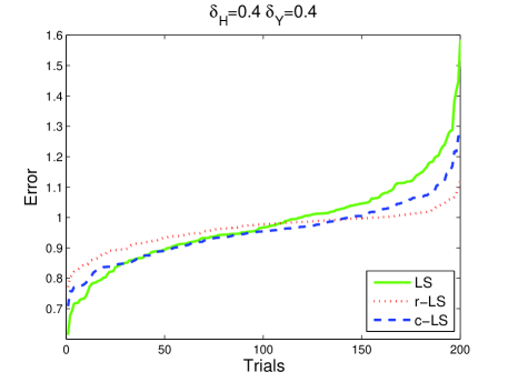
Note that the LS algorithm yields the highest worst case error. Although the worst case error of the c-LS algorithm is larger than the worst case error of the r-LS algorithm, the r-LS algorithm provides a superior performance on the average with respect to both the r-LS and the LS algorithms.

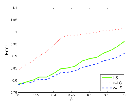
For the second experiment, we randomly generate $200$ random perturbations $\Delta\mbox{$\mathbf{H}$}$, $\Delta\mbox{$\mathbf{y}$}$, where $\lVert\Delta\mbox{$\mathbf{H}$}\rVert\leq\mbox{$\delta$}_{H}$, $\lVert\Delta\mbox{$\mathbf{y}$}\rVert\leq\mbox{$\delta$}_{Y}$, $m=5$, $n=3$ for different perturbation bounds and compute the averaged error over $200$ trials for the c-LS, the LS, and the r-LS algorithms. In Fig. 2, we present the averaged LS errors for the c-LS, the LS, and the c-LS algorithms where the perturbation bound varies, $\delta_{Y}=\delta_{H}=\delta\in[0.3,0.6]$. We observe that the proposed c-LS algorithm has the best average LS error performance over different perturbation bounds compared to the LS and r-LS algorithms.

Refer to caption
Figure 3: Sorted errors for sr-LS, sc-LS, SLS-BDU, and LS algorithms over 100 trials when $\mbox{$\delta$}_{H}=\mbox{$\delta$}_{Y}=0.4$.
Refer to caption
Figure 4: Sorted errors for r-RLS, s-RLS and RLS algorithms over 1000 trials when $\mbox{$\delta$}_{Y}=\mbox{$\delta$}_{H}=0.3$.

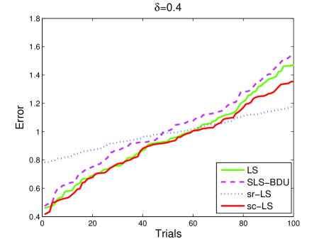
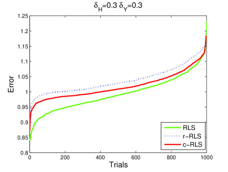
In the next experiment, we examine a system identification problem [2], which can be formulated as $\mbox{$\mathbf{U}$}_{0}\mbox{$\mathbf{h}$}=\mbox{$\mbox{$\mathbf{y}$}$}_{0}$, where $\mbox{$\mathbf{U}$}=\mbox{$\mathbf{U}$}_{0}+\mbox{$\mathbf{W}$}$ is the observed noisy Toeplitz matrix and $\mbox{$\mbox{$\mathbf{y}$}$}=\mbox{$\mbox{$\mathbf{y}$}$}_{0}+\mbox{$\mbox{$\mathbf{w}$}$}$ is the observed noisy output vector. Here, the convolution matrix $\mathbf{U}$ (which is Toeplitz) constructed from $\mathbf{u}$ which is selected as a random sequence of $\pm 1$’s. For a randomly generated filter $\mathbf{h}$ of length 3, we generate $100$ random structured perturbations for $\mbox{$\mathbf{U}$}_{0}$ and $\mbox{$\mbox{$\mathbf{y}$}$}_{0}$, where $\lVert\mbox{\boldmath$\alpha$}\rVert\leq 0.4\lVert\mbox{$\mathbf{U}$}_{0}\rVert$, and plotted the sorted errors in ascending order in Fig. 3. We observe that the largest errors are 1.53 for the structured least squares bounded data uncertainties, labeled as “SLS-BDU” and presented in [2], 1.47 for the LS algorithm, 1.35 for the structured regret LS algorithm “sc-LS” from the Corollary, and 1.17 for the structured robust LS algorithm “sr-LS”. We observe that the sr-LS algorithm yields the largest error on the average, however, it yields the smallest worst case error among other algorithms as expected. In addition, we observe that the sc-LS algorithm has a smaller worst case error compared to the LS and the SLS-BDU algorithms, and it has the smallest average error compared to the sr-LS, the SLS-BDU, and the LS algorithms, justifying its competitiveness in these simulations. Finally, in Fig. 4, we provide data errors sorted in ascending order for the algorithm in Theorem 2 as “c-RLS”, for the robust regularized LS algorithm in [3] as “r-RLS” and finally for the regularized LS algorithm as “RLS[4], where the experiment setup is the same as in the first experiment except the number of trials is 1000 and the perturbation bound is 0.3. The regularization parameter is chosen as $\mu=0.1$. In these simulations, we observe that the c-RLS algorithm trades off performance between the r-RLS and the RLS algorithms. The RLS algorithm yields the largest error compared to the r-RLS and c-RLS algorithms and we observe that although c-RLS has an inferior performance compared to the RLS algorithm on the average it yields a superior performance than the r-RLS algorithm.

V Conclusion

In this correspondence, we introduced a novel robust approach to LS problems with bounded data uncertainties based on a certain regret formulation. We investigated the LS problems for both unstructured and structured perturbations, and the robust regularized LS problem for unstructured perturbations. In each case, the data vectors that minimize the worst case regrets are found by solving certain SDP problems. In our simulations, we observed that the proposed algorithms provide a fair trade off between performance and robustness, better than the best available alternatives in different signal processing applications. Proof of Theorem 1: By applying S-procedure [5] to (4), and with some algebra one can show that (4) is equivalent to solving the following SDP problem

$$\min\mbox{$\gamma$}\mbox{ subject to}$$
$$0\leq\left[\begin{array}[]{cc}\mbox{$\gamma$}+\mbox{$\xi$}+\mbox{$\mathbf{c}$}^{T}\mbox{$\mathbf{h}$}+\mbox{$\mathbf{h}$}^{T}\mbox{$\mathbf{c}$}+\Delta\mbox{$\mathbf{y}$}^{T}\mbox{$\mathbf{b}$}+\mbox{$\mathbf{b}$}^{T}\Delta\mbox{$\mathbf{y}$}&\left(\mbox{$\tilde{\mbox{$\mathbf{H}$}}$}\mbox{$\mbox{$\mathbf{u}$}$}-\mbox{$\tilde{\mbox{$\mathbf{y}$}}$}\right)^{T}\\ \left(\mbox{$\tilde{\mbox{$\mathbf{H}$}}$}\mbox{$\mbox{$\mathbf{u}$}$}-\mbox{$\tilde{\mbox{$\mathbf{y}$}}$}\right)&\mbox{$\mathbf{I}$}\end{array}\right].$$ (23)

Rearranging terms in (23) results

$$-\left[\begin{array}[]{c}\mbox{$\mathbf{c}$}^{T}\\ \mbox{$\mathbf{U}$}\end{array}\right]\mbox{$\mathbf{h}$}\left[\begin{array}[]{cc}1&\mbox{$\mathbf{0}$}\end{array}\right]-\left[\begin{array}[]{c}1\\ \mbox{$\mathbf{0}$}\end{array}\right]\mbox{$\mathbf{h}$}^{T}\left[\begin{array}[]{cc}\mbox{$\mathbf{c}$}&\mbox{$\mathbf{U}$}^{T}\end{array}\right]\leq\left[\begin{array}[]{cc}\mbox{$\gamma$}+\mbox{$\xi$}+\Delta\mbox{$\mathbf{y}$}^{T}\mbox{$\mathbf{b}$}+\mbox{$\mathbf{b}$}^{T}\Delta\mbox{$\mathbf{y}$}&\left(\mbox{$\mbox{$\mathbf{H}$}$}\mbox{$\mbox{$\mathbf{u}$}$}-\mbox{$\tilde{\mbox{$\mathbf{y}$}}$}\right)^{T}\\ \left(\mbox{$\mbox{$\mathbf{H}$}$}\mbox{$\mbox{$\mathbf{u}$}$}-\mbox{$\tilde{\mbox{$\mathbf{y}$}}$}\right)&\mbox{$\mathbf{I}$}\end{array}\right].$$ (24)

Here we used the identity $\Delta\mbox{$\mathbf{H}$}\mbox{$\mbox{$\mathbf{u}$}$}=\mbox{$\mathbf{U}$}\mbox{$\mathbf{h}$}$, where $\mbox{$\mathbf{h}$}=\mathrm{vec}\left(\Delta\mbox{$\mathbf{H}$}\right)$. If we apply Proposition 2 of [7] into (24), we obtain

$$-\left[\begin{array}[]{c}\mbox{$\mathbf{b}$}^{T}\\ -\mbox{$\mathbf{I}$}\\ \mbox{$\mathbf{0}$}\end{array}\right]\Delta\mbox{$\mathbf{y}$}\left[\begin{array}[]{ccc}1&\mbox{$\mathbf{0}$}&\mbox{$\mathbf{0}$}\end{array}\right]-\left[\begin{array}[]{c}1\\ \mbox{$\mathbf{0}$}\\ \mbox{$\mathbf{0}$}\end{array}\right]\Delta\mbox{$\mathbf{y}$}^{T}\left[\begin{array}[]{ccc}\mbox{$\mathbf{b}$}&-\mbox{$\mathbf{I}$}&\mbox{$\mathbf{0}$}\end{array}\right]\leq\left[\begin{array}[]{ccc}\mbox{$\gamma$}+\mbox{$\xi$}-\tau&\left(\mbox{$\mbox{$\mathbf{H}$}$}\mbox{$\mbox{$\mathbf{u}$}$}-\mbox{$\mbox{$\mathbf{y}$}$}\right)^{T}&\mbox{$\delta$}_{H}\mbox{$\mathbf{c}$}^{T}\\ \left(\mbox{$\mbox{$\mathbf{H}$}$}\mbox{$\mbox{$\mathbf{u}$}$}-\mbox{$\mbox{$\mathbf{y}$}$}\right)&\mbox{$\mathbf{I}$}&\mbox{$\delta$}_{H}\mbox{$\mathbf{U}$}\\ \mbox{$\delta$}_{H}\mbox{$\mathbf{c}$}&\mbox{$\delta$}_{H}\mbox{$\mathbf{U}$}^{T}&\tau\mbox{$\mathbf{I}$}\end{array}\right].$$ (25)

Applying Proposition 2 of [7] again in (25) yields (5). $\square$

References

  • [1] L. El Ghaoui and H. Lebret, “Robust solutions to least-squares problems with uncertain data,” SIAM Journal Matrix Analysis and Applications, October 1997.
  • [2] M. Pilanci, O. Arikan, and M.C. Pinar, “Structured least squares problems and robust estimators,” IEEE Trans. on Signal Process., vol. 58, no. 5, pp. 2453 –2465, May 2010.
  • [3] A. H. Sayed, V. H. Nascimento, and F. A. M. Cipparrone, “Structured least squares problems and robust estimators,” SIAM J. Matrix Analysis and Applications, vol. 23, no. 4, pp. 1120–1142, May 2002.
  • [4] T. Kailath, A. H. Sayed, and B. Hassibi, Linear Estimation, Prentice-Hall, 2000.
  • [5] S. Boyd, L. El Ghaoui, E. Feron, and V. Balakrishnan, Linear Matrix Inequalities in System and Control Theory, Studies in Applied Mathematics, 1994.
  • [6] M. Pilanci and O. Arikan, “Recovery of sparse perturbations in least squares problems,” in IEEE International Conference on Acoustics, Speech and Signal Processing, May 2011, pp. 3912–3915.
  • [7] Y.C. Eldar and N. Merhav, “A competitive minimax approach to robust estimation and random parameters,” IEEE Trans. on Signal Process., vol. 52, no. 7, pp. 1931–1946, July 2004.
  • [8] Y.C. Eldar, A. Ben-Tal, and A. Nemirovski, “Linear minimax regret estimation of deterministic parameters with bounded data uncertainties,” IEEE Trans. on Signal Process., vol. 52, no. 8, pp. 2177 – 2188, August 2004.
  • [9] Y.C. Eldar and N. Merhav, “Minimax mse-ratio estimation with signal covariance uncertainties,” IEEE Trans. on Signal Process., vol. 53, no. 4, pp. 1335 – 1347, April 2005.
  • [10] S.S. Kozat and A.T. Erdogan, “Competitive linear estimation under model uncertainties,” IEEE Trans. on Signal Process., vol. 58, no. 4, pp. 2388 –2393, April 2010.
  • [11] A. Graham, Kronecker Products and Matrix Calculus: with Applications, John Wiley and Sons, 1981.
  • [12] D. Vernon (Ed.), Computer Vision - ECCV 2000, 6th European Conference on Computer Vision, Dublin, Ireland, June 26 - July 1, 2000, Proceedings, Part I. Lecture Notes in Computer Science, Springer, 2000.