The gravitational instability of a stream of co-orbital particles

Abstract

We describe the dynamics of a stream of equally spaced macroscopic particles in orbit around a central body (e.g. a planet or star). A co-orbital configuration of small bodies may be subject to gravitational instability, which takes the system to a spreading disordered and collisional state. We detail the linear instability’s mathematical and physical features using the shearing sheet model and subsequently track its nonlinear evolution with local N-body simulations. This model provides a convenient tool with which to understand the gravitational and collisional dynamics of narrow belts, such as Saturn’s F-ring and the streams of material wrenched from tidally disrupted bodies. In particular, we study the tendency of these systems to form long-lived particle aggregates. Finally, we uncover an unexpected connection between the linear dynamics of the gravitational instability and the magnetorotational instability.

1 Introduction

This paper is concerned with the gravitational and collisional dynamics of belts of material orbiting planets or stars. Of particular interest are Saturn’s F-ring and the tidal streams torn from disrupted satellites. The F-ring is thought to comprise a population of large objects (of some 10 km) swathed in dust (Showalter 2004, Esposito et al. 2008, Murray et al. 2008). Being located so near the Roche limit, the size distribution of these larger bodies evolves according to gravitational aggregation, and tidal and collisional disruption (Barbara and Esposito 2002, Esposito et al. 2012). The tidal environment is very different for those dense narrow rings located interior the Roche limit, such as the $\epsilon$-ring of Uranus or the dense ringlets ensconced in Saturn’s C-ring (Colwell et al. 2009). It is possible that these dense ringlets originated from the tidal disruption of small satellites (or the mantles thereof), with their early evolution controlled by gravitational instabilities (Leinhardt et al. 2012).

We would like to understand these several processes — tidal disruption, particle clumping, gravitational instability, collisions — in a single theoretical framework using a simple but illuminating analytical model and N-body simulations. The main configuration that we consider is the gravitational stability of a stream, or line, of many equally spaced particles. To facilitate its study, we employ a local model: the shearing sheet. In doing so we can more easily reproduce the famous result of Maxwell’s Adams Prize essay (Maxwell 1859, Cook and Franklin 1964) and form a more intuitive understanding of the instability’s physics. We find a stream of particles is susceptible to two kinds of disruption: a familiar gravitational clumping instability, and a growing epicyclic mode. Which instability the system selects depends on a single dimensionless parameter analogous to the Roche parameter that controls the tidal disruption of a satellite.

The nonlinear outcome of these instabilities is studied with N-body simulations using the code REBOUND (Rein and Liu 2012). We find that the precise form of the initial instability is unimportant; instead, the nonlinear evolution is entirely controlled by the tendency of the system to form particle aggregates. Existing clustering criteria are discussed (Weidenschilling et al. 1984, Ohtsuki 1993, Canup and Esposito 1995), and we simulate an interesting intermediate regime relevant to Saturn’s outer rings, whereby collisional aggregation is rare, but not impossible, and instead particles form temporary short-lived clusters (cf. ‘dynamical ephemeral bodies’, Weidenschilling et al. 1984).

These gravitational instabilities may illuminate other astrophysical contexts. For instance, the mechanism of instability we outline here could also be at work in the non-axisymmetric instabilities of narrow fluid rings and slender tori (Maxwell 1859, Goodman and Narayan 1988, Papaloizou and Lin 1989). It also manifests in the ‘propeller and frog’ resonance of Pan and Chiang (2010, 2012) which aims to describe the observed migration of large embedded objects (propellers) in Saturn’s A-ring. If the propeller is permitted to back-react on the rest of the ring, then an instability will arise, analogous to the one we study here. Lastly we show how the mechanism of instability in the growing epicyclic mode, relying on significant angular momentum exchange, shares some of the mathematical and physical characteristics of the magnetorotational instability (MRI) (Balbus and Hawley 1991). In fact, the two instabilities are nearly identical for a certain (somewhat artificial) equilibrium set-up.

The following section outlines the linear theory of the gravitational instability, connecting it to previous work by Maxwell (1859) and Fermi and Chandrasekhar (1953), while showing its similarities to the MRI. Section 3 presents N-body simulations of the instability’s nonlinear and collisional evolution. In Section 4 we summarise our results.

2 Linear Theory

2.1 Governing equations and setup

Consider a train of spherical particles in a circular orbit around a point mass or around a central mass with a point-mass potential. The particles initially inhabit the same orbital radius but are equally spaced in azimuth by a distance $h$. Each particle has the same mass $m$ which is much smaller than the central mass. If the spacing $h$ is sufficiently small and the ensuing dynamics remain confined to lengthscales much less than the orbital radius, we may adopt the shearing sheet model or local approximation (Goldreich and Lynden-Bell 1965), in which case we can write down the equations of motion for each particle in a convenient way. The shearing sheet is anchored at a radius $R_{0}$ from the central object around which it orbits with frequency $\Omega$. In this model, the motion of particle $n$ is governed by

$$\ddot{x}_{n}-2\Omega\dot{y}_{n} =3\Omega^{2}\,x_{n}+f_{x}^{n},$$ (1)

$$\ddot{y}_{n}+2\Omega\dot{x}_{n} =f_{y}^{n},$$ (2)

$$\ddot{z}_{n} =-\Omega^{2}\,z_{n}+f_{z}^{n},$$ (3)

where $(x_{n},\,y_{n},\,z_{n})$ denotes the coordinates of particle $n$ in the shearing box relative to the reference position $R_{0}$, an overdot indicates a time derivative, and $\mathbf{f}^{n}$ is the specific collective gravitational force of all the other particles on particle $n$. The gravitational force may be written as

$$\mathbf{f}^{n}=G\,m\sum_{j\neq n}\frac{\Delta x_{jn}\mathbf{e}_{x}+\Delta y_{jn}\mathbf{e}_{y}+\Delta z_{jn}\mathbf{e}_{z}}{[\Delta x_{jn}^{2}+\Delta y_{jn}^{2}+\Delta z_{jn}^{2}]^{3/2}},$$ (4)

where the sum is over all other particles, with $G$ as the gravitational constant, and the distances

$$\Delta x_{jn}=x_{j}-x_{n},\quad\Delta y_{jn}=y_{j}-y_{n},\quad\Delta z_{jn}=z_{j}-z_{n}.$$

In reality there are a large but finite number of particles in the ring, but in practice we take the above sum to be infinite and so $j$ runs between $-\infty$ and $\infty$. Even if the force is approximated as an infinite sum, it remains convergent because only nearby particles significantly influence any given particle’s dynamics. See Salo and Yoder (1988) or Vanderbei and Koleman (2007) for a discussion of situations in which the rings contain only a few massive particles.

2.2 Equilibrium

This set of equations admits as an equilibrium state a procession of equally spaced particles located in the central axis of the sheet, i.e. for

$$x_{n}=0,\quad y_{n}=hn,\quad z_{n}=0,\qquad\forall\,n\in\mathbb{Z},$$ (5)

where $h$ is the azimuthal spacing. The force $\mathbf{f}^{n}$ is zero for each $n$: the gravitational influences of the particles preceding a given particle $n$ are cancelled exactly by all the particles trailing particle $n$.

2.3 Linearised equations

We next perturb this stream of particles by a set of small displacements $(x_{n}^{\prime},\,y_{n}^{\prime})$ that lie only in the orbital plane. Vertical displacements are neglected as they decouple in the linear regime and do not lead to instability. The linearised equations for these time-dependent displacements are:

$$\ddot{x}_{n}^{\prime}-2\Omega\dot{y}_{n}^{\prime}-3\Omega^{2}x_{n}^{\prime}=\frac{Gm}{h^{3}}\sum_{j=-\infty}^{\infty}\frac{x_{j}^{\prime}-x_{n}^{\prime}}{|j-n|^{3}},$$ (6)

$$\ddot{y}_{n}^{\prime}+2\Omega\dot{x}_{n}^{\prime}=-2\frac{Gm}{h^{3}}\sum_{j=-\infty}^{\infty}\frac{y^{\prime}_{j}-y^{\prime}_{n}}{|j-n|^{3}}\,,$$ (7)

where both sums omit the $j=n$ term.

We now suppose the particle motions assume a collective Fourier mode of the type

$$x_{n}^{\prime}=X\,\text{e}^{st+nhk\text{i}},\qquad y_{n}^{\prime}=Y\,\text{e}^{st+nhk\text{i}},$$

with $X$ and $Y$ complex amplitudes, $s$ a growth rate (complex in general), and $k$ a (real) wavenumber. In order to avoid aliasing, the magnitude of $k$ is restricted to be equal or less than $\pi/h$. The equations reduce to two,

$$s^{2}X-2\Omega sY-3\Omega^{2}X=-\frac{Gm}{h^{3}}F\,X,$$ (8)

$$s^{2}Y+2\Omega sX=2\frac{Gm}{h^{3}}F\,Y,$$ (9)

in which we have introduced the dimensionless force function $F$. It can be manipulated into

$$F(K)=2\sum_{j=1}^{\infty}\frac{1-\cos(j\,K)}{j^{3}},$$ (10)

where we have introduced a dimensionless wavenumber $K=hk$. The force function depends only on $K$, and can be re-expressed in terms of the zeta and Clausen functions (Lewin 1981). We find that $F>0$ and is an increasing function of $K$, with $F\to 0$ as $K\to 0$. The following asymptotic expansion, for small $K$, offers a reasonable approximation for all physical wavenumbers:

$$F=\left(\frac{3}{2}-\ln K\right)\,K^{2}+\frac{1}{96}\,K^{4}+\mathcal{O}(K^{6}),$$

(for a derivation see, for example, Nicorovici et al. 1994).

2.4 Springs, clumping, and angular momentum exchange

Before moving on to the dispersion relation itself, we make some preliminary remarks. First, if the central object and the orbital motion are neglected, the terms involving $\Omega$ in Eqs (8) and (9) disappear. Consequently, the azimuthal and radial motions decouple and the azimuthal equation gives rise to an unstable longitudinal mode which tends to clump particles together. Its growth rate is clear from inspection and is equal to $\sqrt{2GmF/h^{3}}$. This unstable mode, which grows as the result of a release of gravitational potential energy, is the discrete analogue of the instability of an infinite self-gravitating cylinder described by Chandraskehar and Fermi (1953) (see also Chandrasekhar 1981).

Second, (8) and (9) are reminiscent of the equations governing two orbiting bodies attached by a spring, as popularised by Balbus in his interpretation of the magnetorotational instability (Balbus and Hawley 1991). There is, however, a crucial difference in that our ‘gravitational spring constant’ differs in both size and sign depending on the direction of the spring force. While the gravitational ‘spring’ seeks to resist extension in the radial direction (as in the MRI), it actively encourages it in the longitudinal direction. In some sense, the spring wants to become ‘clumpy’. At the same time the spring forces also facilitate angular momentum exchange, which introduces a separate route to instability, employed by the MRI and the Papaloizou-Pringle instability (Papaloizou and Pringle 1984). Outward angular momentum transfer liberates orbital energy which is channeled into exponential growth. The gravitational instabilities we study in this paper are the outcome of the interplay, and sometimes competition, between these two instability mechanisms.

2.5 Dispersion relation

We rescale time so that $\Omega=1$. Eliminating $X$ and $Y$ from Eqs (8) and (9) yields the following dispersion relation for $s$:

$$s^{4}+[1-gF(K)]s^{2}+2gF(K)[3-gF(K)]=0,$$ (11)

where we have introduced the important dimensionless quantity

$$g=\frac{(m/h^{3})\,G}{\Omega^{2}}.$$ (12)

It measures the influence of the stream’s self-gravity relative to its inertial forces.

The $g$ parameter bears a superficial resemblance to the ‘Roche parameter’ of an orbiting fluid satellite vulnerable to tidal disruption:

$$\mathcal{R}=\pi\frac{\rho\,G}{\Omega^{2}},$$ (13)

where $\rho$ is the mass density of the satellite. We find gravitational instability favours larger $g$ — hence greater mass densities and greater radii, $R_{0}$. In contrast, a larger $\mathcal{R}$ in the Roche problem corresponds to a greater resistance to disruption (Chandrasekhar 1987). This reflects the fact that the inertial forces are stabilising in the ring context and disruptive in the satellite context. As we show later, however, the parameter $g$ does not control the nonlinear saturation of gravitational instability.

Finally, note that by making the identification $gF(K)=v_{A}^{2}k^{2}/\Omega^{2}$, where $v_{A}$ denotes Alfvén speed, Eq. (11) becomes strikingly similar to the MRI dispersion relation (e.g. Eq. (79) in Balbus 2003). But differences in sign occur at key places, which we associate with the tendency to azimuthally clump.

2.6 Fastest growing modes and stability criterion

In this problem the shortest modes are the most unstable: they always grow the fastest and they are always the first to be destabilised. Therefore, our stability considerations need only make reference to these short scales. The shortest modes possess $K=\pi$ and the force function is, consequently, $F(\pi)=(7/2)\zeta(3)\approx 4.2$, where $\zeta(3)$ is Apéry’s constant. From the explicit solution to the (bi-) quadratic (11), we find three bifurcations as $g$ varies. In order of increasing $g$, these occur at

$$g=\frac{26\pm 8\sqrt{10}}{63\,\zeta(3)}\approx 0.00927,\,0.677,$$ (14)

and

$$g=\frac{6}{7\zeta(3)}\approx 0.714.$$ (15)

The first bifurcation corresponds to the onset of instability. When $g<0.00927$ there exist only neutral modes, and the system is stable. Two of the modes in this regime consist of near-epicyclic motion with frequency $|s|\lesssim\Omega$. As $g$ is increased through $0.00927$, there is a Hopf bifurcation and both these oscillations pick up equal and positive growth rates (in addition, there are decaying modes as the system is Hamiltonian). The gravitational instability takes the rather novel form of a pair of growing epicycles (as in the viscous overstability — Borderies et al. 1985, Schmit and Tscharnuter 1995, Latter and Ogilvie 2009). Note that the stability criterion, $g<0.00927$, can be reformulated into the following:

$$\frac{m}{M}<2.298657/N^{3},$$ (16)

where $N$ is the total number of particles and $M$ is the mass of the central object. Here we have defined the number of particles through $Nh=2\pi R_{0}$. Equation (16) is the famous stability criterion that Maxwell derived in his Adams Prize essay for the stability of $N$ co-orbital particles for large $N$ (Maxwell 1859, Cook and Franklin 1964).

Now, when $g$ is increased towards $0.677$, the next critical value, the oscillation frequencies of the two unstable modes are gradually suppressed by the self-gravity. At $g=0.677$ these oscillation frequencies are precisely zero, and there exists a double root to (11). When $g>0.677$ both unstable modes are monotonically growing, and cease to oscillate. As $g$ is increased further, these two modes decouple: one growing more quickly than the other. Eventually, when $g>0.714$ (the third bifurcation), the slower of the two becomes neutral, leaving only one growing mode. The instability now takes the more familiar form of longitudinal clumping. This is especially clear in the limit of large $g$, where the unstable mode’s growth rate approaches $\sqrt{2g\,F(\pi)}$, which is the value for a non-orbiting line of self-gravitating particles (cf. Section 2.4) .

2.7 Modes of general wavelength

Modes on longer scales (smaller $K$) follow the same pattern, though the critical values of $g$ are larger, and are different for each $K$. Note that sufficiently long modes are always stable for any given $g$. Once we stipulate $g$ — no matter how large — formally we can always find a sufficiently small $K$ so that $gF(K)\ll 1$. (In reality, of course, $K$ is limited by the circumference of the ring.) Expanding (11) in this small combination gives the growth rates:

$$s=\pm i\left[\sqrt{6gF}+\mathcal{O}(gF)\right],\quad s=\pm i\left[1+\mathcal{O}(gF)\right].$$ (17)

The instability scale is tied to the strength of self-gravity. Conversely, in the MRI context, once the strength of the imposed magnetic field is specified (via the Alfvén speed), we may always find a wavelength above which the MRI operates. In the gravitational instability, once the strength of the particles’ self-gravity is specified, we may always find a wavelength below which the GI operates (but only when $g>0.00927$).

2.8 Growth rates

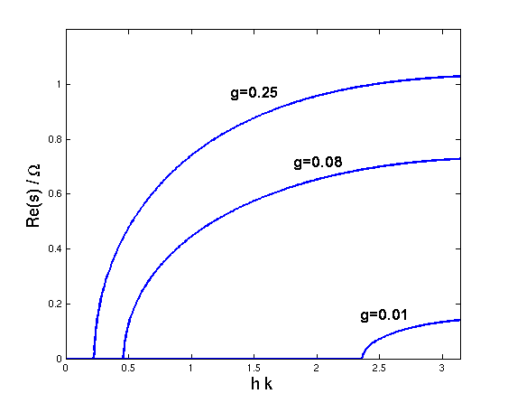
Figure 1: Growth rates of the gravitational instability as a function of dimensionless wavenumber $K$ for three different $g=$ 0.01, 0.08, and 0.25. Each curve is labelled with its corresponding value of $g$. There are two unstable modes with the same growth rate and both oscillating with a frequency $\approx\pm\Omega$.

In Fig. 1, we plot the real part of the growth rate $s$ of the unstable modes as a function of $K$, for various $g$. In this figure we concentrate on the growing epicycles; thus we limit $g$ to be less than $g<0.677$. Three values of $g$ are chosen: 0.01, 0.08, and 0.25. As explained earlier, the shortest modes (largest $K$) modes are the most unstable, but $K\leq\pi$. Note finally that for sufficiently long modes instability is quenched in all three cases.

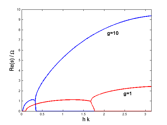
Figure 2: Growth rates as functions of $K$ for larger values of $g$. Two values are chosen: $g=1,\,10$. Above a critical $K$, in both cases, there exists only one monotonically growing mode. For $K$ below a second critical value, there are two unstable epicyclic modes growing at the same rate. This value occurs at the ‘branches’ in the dispersion relation. For $K$ less than a third critical value the modes are stable.

In Fig. 2, we extend the previous plot to larger $g$, in which we find the instability taking the form of gravitational clumping on shorter scales. Two values of $g$ are chosen above the value $0.677$. In both cases instability is quenched for small $K$. One may also observe the bifurcation at a second critical $K$ at which point the instability changes from being two growing epicycles, to two monotonic clumping modes. For $K$ greater than a slightly larger value, one of these modes stabilises, and only one growing mode remains.

2.9 Physical interpretation

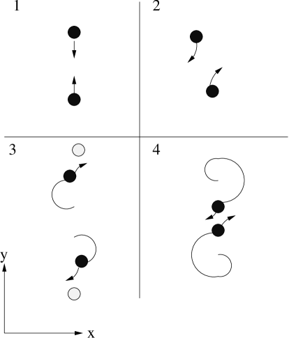
Figure 3: A cartoon of the onset of oscillatory instability. The first panel shows two adjacent particles given a small displacement toward one another. In the second, their mutual attraction gives rise to an epicyclic motion (akin to a ‘horseshoe’ turn), the amplitude of which is increased by a gravitational encounter with the particles on either side of the pair, shown in the third panel. In the last panel, the two particles kick each other once again giving rise to an even large (modified) epicyclic motion.

The instability associated with longitudinal clumping, at larger $g$, is relatively straightforward to understand. A pattern of compression and rarefaction is self-amplifying because gravitational attraction increases when neighbouring particles are displaced closer to each other. In contrast, the ‘epicyclic’ instability, which occurs for smaller values of $g$, relies on a mechanism that is a little more subtle and which we now describe using a simple cartoon.

Consider the four ‘snapshots’ of Fig. 3. In the first panel, we have drawn just two particles within the initial equilibrium state. These two particles have been displaced slightly towards each other (and away from their other immediate neighbours). As a result, there is a net gravitational attraction between them (the black arrows). This force ‘slows down’ the leading particle and ‘speeds up’ the trailing particle; thus an angular momentum exchange takes place. Consequently, both particles begin an epicycle around the two new radii that are associated with their new angular momenta: the leading particle moves to a smaller radius, while the trailing moves to a larger radius (Panel 2). Note that if the gravitational attraction is sufficiently strong (large $g$) then the particles would clump or collide before the epicyclic motion gets properly underway. Panel 3 describes what happens when the two particles complete half of their epicycle. At this stage they are closer to their other near neighbours (in white) than to each other. Both subsequently receive a second attractive force from the white particles that sends them into new (larger) epicycles. Finally, when our two black particles return to their initial radius (panel 4), they are azimuthally closer to each other than when they began (in panel 1). Their gravitational attraction is now stronger and sends them into new epicycles of greater amplitude, and the process runs away. Thus the instability relies on a sequence of gravitational encounters between neighbouring elements; and these act as an ‘epicyclic amplifier’.

The amplifier we describe here should be contrasted with the ‘propeller and frog’ resonance (Pan and Chiang 2010). In the set-up of Pan and Chiang, two ‘particles’ are held fixed ahead of and behind a third particle. This third particle, when displaced, feels the gravitational attraction of the other two, but does not act back upon them. Consequently, it undergoes a periodic epicyclic-like motion of a steady amplitude. However, as soon as we let the third particle react back on its two chaperones, an instability of the type we describe above should occur. Recently this seems to have been observed (Pan and Chiang 2012).

2.10 A gravitational analogue of the MRI

Before we move on to the nonlinear development of the gravitational instability, it is of interest to briefly examine a different but related model of instability, in which the dynamics of the incompressible MRI are reproduced in most of their details.

Consider, instead of a stream of particles extended along the azimuthal direction, a vertical line of particles located at a single radius and azimuth: $x_{n}=y_{n}=0$. The particles are equally spaced in $z$. However, in order to keep this configuration in equilibrium it is necessary to ‘switch-off’ the vertical tidal force of the central object in Eq. (3). It is also necessary to assume that the vertical line of particles is extremely long and that we study only particles at the midplane far from the unbalanced ends. This ‘equilibrium’ may then be written as

$$x_{n}=0,\quad y_{n}=0,\quad z_{n}=hn,\qquad\forall n\in\mathbb{Z}.$$

As before, we consider only linear planar disturbances to this basic state, and we describe this perturbation by

$$(x_{n}^{\prime},\,y_{n}^{\prime},\,0)=(X,\,Y,\,0)\,\text{e}^{st+nK\text{i}}.$$

Its linearised equations read

$$s^{2}X-2\Omega sY-3\Omega^{2}X=-\frac{Gm}{h^{3}}F\,X,$$ (18)

$$s^{2}Y+2\Omega sX=-\frac{Gm}{h^{3}}F\,Y,$$ (19)

where $F$ is given earlier in Eq. (10).

Equations (18)-(19) describe two bodies connected by a spring, with a single spring constant $(Gm/h^{3})F(K)$. The linear dynamics of the incompressible MRI can be described in precisely the same way if $v_{A}^{2}k^{2}$ is substituted for the spring constant (Balbus 2003). Under this substitution, the dispersion relations of the MRI and gravitational instability are almost identical! The only difference comes from $F$’s dependence on wavenumber, which is more complicated than $k^{2}$. Yet like $k^{2}$, it is an increasing function and goes to 0 as $k\to 0$.

So in this toy problem we have managed to reproduce the MRI dynamics by letting the gravitational force between particles do the job of magnetic tension in the MRI. And by extending the particles in the $z$-direction but suppressing their vertical motion we can nullify gravity’s tendency to clump the particles (the complicating process in Section 2.4). Particles at different $z$ are drawn apart from each other in the plane; but these displacements engender planar gravitational torques that transport angular momentum from particles at smaller radii to particles at larger radii. Particles then drift further apart, angular momentum is further exchanged, and the process runs away. The system develops a vertical sequence of planar jets, or ‘channel flows’, as in the MRI (Goodman and Xu 1984). Unlike the MRI, however, these flows are not nonlinear solutions to the equations of motion.

3 Nonlinear and collisional evolution

In this section we present three-dimensional N-body simulations of the nonlinear and collisional evolution of the gravitational instabilities discussed. The equations (1)-(3) are numerically evolved forward in time in a corotating local frame, which imposes a finite periodicity in the azimuthal ($y$) direction, but has no radial boundaries. Unlike the shearing box, particles cannot leave the box through one radial boundary and reappear through the other. The simulations can show how the saturation of the instability depends on the governing parameters of the system, and if the eventual outcome of the clumping form of the instability differs from the outcome of its oscillatory form.

3.1 Parameters

In addition to the dimensionless parameter $g$, which governs the linear stage, N-body simulations introduce three more parameters associated with the collisional energy losses, the particle diameter, and the number of particles $N$ in the box. We, however, have verified that our results do not depend on $N$, which has no direct physical meaning. Particles are assumed to be non-spinning inelastic spheres endowed with a constant normal coefficient of restitution, $\epsilon$. Therefore

$$v_{n}^{\prime}=-\epsilon\,v_{n},$$ (20)

where $v_{n}$ and $v_{n}^{\prime}$ denote the normal relative velocities of two colliding particles before and after the collision respectively.

The particles’ diameter we denote by $d$, which suggests a dimensionless parameter analogous to $g$. For consistency with previous work (Ohtsuki 1993, Canup and Esposito 1995), we use the ratio

$$r_{p}=\frac{d}{r_{\text{H}}}=\left(\frac{2G\,m}{3d^{3}\,\Omega^{2}}\right)^{-1/3},$$ (21)

where $r_{\text{H}}$ is the mutual Hill radius of the particles. The parameter $r_{p}$ may be recast as

$$r_{p}=12^{1/3}\left(\frac{\rho_{c}}{\rho_{p}}\right)^{1/3}\left(\frac{R_{c}}{R_{0}}\right),$$ (22)

where $\rho_{p}$ is the mass density of a particle, $\rho_{c}$ is the mass density of the central body, with $R_{c}$ denoting its radius. In the case of Saturn’s rings, it follows that $r_{p}<1$ at radii greater than roughly 125,000 km, if we take $\rho_{p}$ to be that of crystalline water ice (900 g/m³). At the radius of the F-ring, $r_{p}$ falls to 0.89.

Finally we can derive the ratio of the particle radius and initial particle spacing from $d/h=0.873\,r_{p}\,g^{1/3}$. Because we must have $d<h$ (or else particles overlap), there is a restriction on the size of $r_{p}$ given $g$, which is easy to calculate: $r_{p}<1.145\,g^{-1/3}$.

3.2 Clustering criteria

The key to the long-term evolution of the ring is the capacity of ring particles to form long-lived aggregates. In this subsection we discuss a number of simple criteria that might help us understand the simulation outcomes.

Initially we consider whether simple aggregates of two particles in contact can resist tidal disruption. The simplest case is that of an aggregate in synchronous rotation, which appears as a non-rotating aggregate in the frame of reference used in this paper. The particle locations are given by $y_{1}=y_{2}=0$ and $x_{1}=-d/2$ and $x_{2}=d/2$. By testing the limiting case of no contact force, Eqs (1) and (2) tell us that this configuration is an equilibrium solution if

$$r_{p}\leq 1,$$ (23)

(Weidenschilling et al. 1984, Longaretti 1989).

This ‘force’ condition provides a clear criterion, but it applies only when two particles are touching in this special configuration. How particles ever reach such an arrangement is not addressed: they may not be all that likely in real collisional systems. Consequently, force criteria may overestimate clump formation. Another approach is taken by Ohtsuki (1993) and Canup and Esposito (1995) who examine the energetics of a collision via the Jacobi integral and compute a condition for accretion during a binary collision. These criteria relate $r_{p}$ and $\epsilon$. Canup and Esposito find that when

$$\epsilon<\sqrt{\frac{v_{e}^{2}+(2/3)r_{p}^{2}-9}{v_{e}^{2}+c^{2}+(2/3)r_{p}^{2}}},$$ (24)

colliding particles should aggregate. Here $v_{e}$ is escape velocity and $c$ is the velocity dispersion of the system. Both are scaled by $r_{\text{H}}\Omega$, and so $v_{e}=\sqrt{6/r_{p}}$. If we assume that $c\sim v_{e}$ in equilibrium, then we have a relationship between $\epsilon$ and $r_{p}$ that tells us whether a typical collision results in aggregation, and hence whether our system has a tendency to become clumpy. In the limit of perfectly dissipative collisions ($\epsilon=0$), which is the most conducive to aggregate formation, the criterion becomes

$$r_{p}\leq 0.691,$$ (25)

significantly less favourable than (23).

These criteria hold only for binary aggregates or binary collisions; but if a binary (or larger) clump has already formed then additional particles can attach themselves to it with greater ease (Weidenschilling et al. 1984). It follows that if criterion (23) is satisfied and yet (24) is not satisfied, a rare event may occur whereby a long-lived aggregate forms and then successfully absorbs other particles, thereby growing larger and larger. For fixed $\epsilon$, it follows that an intermediate regime may exist, with $r_{p}$ lying between the limits obtained from (24) and (23) (Salo 1995). For $\epsilon=0$, this would be $0.691<r_{p}<1$. In this regime long-lived clumps do not form in general — almost all collisions do not result in capture — but given sufficient time a rare particle encounter occurs that does result in an aggregate. This aggregate may then grow successfully, an embedded blob in an otherwise monodisperse ring.

3.3 Numerical method

Using the collisional N-body code REBOUND (Rein and Liu 2012) we study the gravitational instability by directly evolving Eqs. (1)-(3). Because of the small number of particles, we can use direct summation to accurately calculate self-gravity and do not have to use a tree or FFT-based gravity solver.

We use the mixed-variable symplectic epicycle integrator SEI (Rein and Tremaine 2011) which is ideally suited for this study. A symplectic integrator does not introduce artificial trends in formally conserved quantities. The mixed-variable integrator gives a large accuracy gain when the particle motion is dominated by epicyclic motion. Because of these properties, we have numerically converged results in most simulations using a time-step as large as one tenth of the dynamical time, $dt=10^{-1}\Omega^{-1}$.

Usually, one employs several ghost boxes in local N-body simulations to ensure that there is no special place in the shearing sheet. The more ghost boxes are used, the better. Here, we find it is sufficient to use only one ghost box in both the positive as well as the negative $y$ direction. There are no ghost boxes in the $x$ direction, since we are dealing with a string of particles. Thus each particle feels the attraction of $3N-1$ other particles.

We pre-calculate the residual force error $E_{i}$ in the calculation of $f_{y}$ comparing the initial numerical setup to a truly infinite string of particles with perfect periodic spacing $h$, cf. Eq. (5). This is similar to the idea of Ewald summation, and the error can be written down explicitly in terms of the first derivative of the digamma function

$$E_{i}=\frac{Gm}{h^{2}}\left(\psi^{\prime}(2N-i)-\psi^{\prime}(1+i+N)\right),$$ (26)

where $i$ is the index of the particle running from $0$ (left) to $N-1$ (right), and a prime denotes differentiation. This error is then subtracted from the numerically calculated forces at every time-step. Using this trick, artificial effects are minimised at the box boundaries even when the instability is followed over many dynamical timescales and grows by many orders of magnitude.

We use an instantaneous collision model. Hence multiple collisions during one time-step may not be treated correctly. Furthermore, we use a minimal impact velocity ($0.05\,d\Omega$ ) so as to avoid overlapping particles when aggregates form. This velocity scale is set much smaller than the velocity dispersion and so should not affect the outcome.

3.4 Linear regime

Figure 4: Largest growth rate of the system in numerical simulations and linear theory as a function of the parameter $g$. Note that the detailed structure at small $g$ is captured perfectly. Here $N=200$.

As a numerical check, the analytic growth rate given by Eq. (11) is verified using the N-body code. We take $N=200$ particles initially lined up in a string and simulate their early evolution. The particles’ location and velocity are perturbed with the unstable eigenfunction of fastest growth. The initial perturbations possess amplitudes of $10^{-7}$ and we stop the evolution when they have grown by 2 orders of magnitude.

In Fig.4 we plot the largest growth rate as a function of the dimensionless parameter $g$. We also show the analytic result from linear theory. One can see that the agreement is excellent, which provides a useful validation of the numerical integrator, and also a check on the analytic theory.

3.5 Nonlinear evolution

Figure 5: Snapshots of a simulation of gravitational instability. Parameters are: $g=0.1$, $r_{p}=0.2$, $\epsilon=0.5$, $N=200$. Note that only a central portion of the computational domain is shown. Particle sizes have been inflated to aid their visualisation; hence particle aggregates appear as overlapping particles. The simulation is initialised by small amplitude random noise.

Figure 6: As in Fig. 5, but with parameters $g=0.1$, $r_{p}=0.8$, $\epsilon=0.5$, $N=200$. .

Long time simulations were ran for a variety of parameters, though first we concentrate on the following four parameter sets presented in Table I.

Case	$g$	$r_{p}$	Instability	Aggregation	$d/h$
(i)	0.1	0.2	Oscill.	Likely	0.081
(ii)	0.1	0.8	Oscill.	Unlikely	0.32
(iii)	1	0.2	Monot.	Likely	0.17
(iv)	1	0.8	Monot.	Unlikely	0.7

Table 1: Parameter sets for the four runs discussed in detail in Section 3.5

In the table, ‘Oscill./Monot. ’ refers to the form of the initial instability, oscillatory or monotonic (determined by $g$), and ‘likely’ or ‘unlikely’ aggregation refers to the likelihood of clumping as decided by (24). In all cases we set $\epsilon=0.5$ and $N=200$. Note that the $r_{p}=0.8$ cases fall within the ‘intermediate regime’ discussed earlier: aggregates can still exist in principle. These parameter choices hence let us observe the potentially different outcomes of the two forms of gravitational instability, while also testing the clustering criteria of Section 3.2.

We find that on medium to long times the simulations yield two typical evolution tracks depending on the parameter $r_{p}$. It appears that after a few orbits the ensuing disordered state retains little memory of the linear instability that gave rise to it. We take simulations (i) and (ii) as examples of these two tracks.

First we treat case (i), as it is the simplest. These parameters yield oscillatory instability and physical collisions that usually lead to capture. In Fig. 5 screenshots of the evolution are presented corresponding to different times. In order to better visualise the results, these images only represent the central portion of the computational domain, comprising initially of 40 particles. Particles are represented by black circles and their radius has been inflated so they are more easily seen. In panel 1, the equilibrium set-up is shown, while in panel 2, the system is on the verge of departing from the linear regime of the oscillatory instability. However, the perturbations are still too small to be easily observed. Panel 3 shows the outcome of the first round of collisions. These initial collisions induce accretion and precipitate disordered non-planar motion in the resulting aggregates. Gravitational encounters liberate orbital shear energy and the ring ‘warms’ up with a velocity dispersion $\sim v_{e}$; in addition, angular momentum is transported and the ring spreads, its width eventually $\propto t^{p}$, for $p$ close to $1/2$. Particles and particle aggregates continue accreting through physical collisions, in accordance with the criterion (24), and after 8 orbits the number of bodies has decreased significantly. Because we have inflated the particle radiuses in the images, the aggregates appear as overlapping circles.

The evolution of case (ii) is represented by eight screenshots in Fig. 6. Unlike case (i), the system does not steadily collapse into a smaller set of aggregates. Instead it swiftly degenerates into a disordered spreading state characterised by a velocity dispersion, as before, of order $v_{e}$ (consistent with Ohtsuki 1999 and Ohtsuki and Emori 2000). The eight panels clearly describe this spreading. However, what they also show is the continuous generation and dissolution of small particle aggregates. Particles come together and then are disrupted by tidal forces, spin, or forceful collisions with other particles. These temporary aggregates resemble the dynamic ephemeral bodies (DEBs) proposed by Weidenschilling et al. (1984). Alternatively, we may think of them as analogues of the gravity wakes exhibited by optically thicker rings (Salo 1992). We have found that some aggregates persist for the length of the simulation. These bodies may have become sufficiently large to pass the tidal disruption threshold for these parameters. Simulations were also run for $r_{p}=0.85,\,0.9,$ and 1 and long-lived clusters failed to appear, though occasional two-particle aggregates were spotted.

These runs confirm an intermediate regime of $r_{p}$ between continuous aggregation and no aggregation at all. This regime is characterised, in particular, by temporary aggregates and by the potential formation of persistent growing clusters that resist disruption amidst the surrounding melee.

3.6 Clumping criterion

In order to measure the efficiency of clustering in detail we conducted a parameter survey of $\epsilon$ and $r_{p}$. We employ a convenient ‘one-dimensional’ measure of the system’s degree of clustering which we now describe. Particles are sorted along the azimuthal direction and the azimuthal distances between neighbouring particles $\Delta y$ calculated. (Their relative radial distances are discarded.) The mean of the resulting distance distribution $\langle\Delta y\rangle$ stays constant throughout a simulation and is equal to $h$. However, its standard deviation will evolve over time. We average this standard deviation over the length of the run and scale it by $h$; the final averaged quantity we denote by $q$ and associate it with the degree of aggregation throughout the run. Note that $q=0$ in the perfectly ordered equilibrium state that we start with, while $q=1$ if the particles are distributed entirely randomly. In the latter case, $\Delta y$ exhibits an exponential distribution with scale parameter $h$. Aggregation corresponds to $q>1$, with $q$ taking its maximum value $q\approx\sqrt{N}$ when all the particles lie in a single cluster. In our simulations, we find that $q$ never exceeds about 6. The one-dimensional measure $q$ is well-suited to a narrow spreading ring, and is also simpler to implement than the two-dimensional Renyi entropy employed in Karjalainen and Salo (2004). Like the Renyi entropy $q$ cannot distinguish between the continuous formation of many temporary clusters and permanent aggregates.

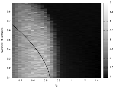
Figure 7: The measure of clumpiness $q$ as a function of $\epsilon$ and $r_{p}$. Superimposed on the greyscale plot is the Canup and Esposito criterion (1995) for gravitational capture after a binary collision (the black line). The other parameters are $g=0.1$ and $N=200$.

Figure 7 plots $q$ in greyscale as a function of $\epsilon$ and $r_{p}$. It summarises 2240 separate simulations each run up to 200 orbits. The figure illustrates clearly the hard boundary at $r_{p}=1$; for larger $r_{p}$, we find $q=1$ and the particles are distributed randomly with little aggregation. Moreover, our results show that aggregation is insignificant until at least $r_{p}\approx 0.8$, though this limit decreases for larger $\epsilon$. The $q$ value jumps abruptly near this critical $r_{p}$, from slightly greater than 1 (little accumulation), to $q\approx 5$, which we associate with the onset of continuous accretion. In addition we have overplotted the Canup and Esposito criterion (1995) given in Eq. (24), which appears to underestimate the prevalence of clustering, especially for higher $\epsilon$.

At small $r_{p}$ it appears that $q$ decreases slightly. This is perhaps due to the fact that in this regime the particles are so small that they rarely collide with each other. Extremely long time integrations are hence required to reach the systems’ accretion time-scales. Our simulations, which were run up to 200 orbits, were perhaps too short. It is also possible that accretion is suppressed in hot rings composed of very small particles.

The numerical results are compatible with self-gravitating simulations of broad rings (Salo 1995, Karjalainen and Salo 2004), which also generate long-lived aggregates. However, the optical depth is much greater in those simulations, and they are significantly perturbed by gravity wakes — conditions that make aggregate formation more likely and more rapid than in our work. In particular, Karjalainen and Salo (2004) find that when $\tau=0.25$ continuous accretion occurs for $r_{p}\lesssim 0.87$ if $\epsilon=0.1$, and for $r_{p}\lesssim 0.85$ if $\epsilon=0.5$. These critical values are larger than ours, but at lower $\tau$ their critical $r_{p}$ approaches 0.8, which is closer to our critical value. It should be noted that these low $\tau$ runs were undertaken with a varying coefficient of restitution.

4 Conclusion

In this paper we have studied the gravitational and collisional dynamics of a stream of co-orbital particles, plotting the course of the system’s evolution from initial instability to its nonlinear saturation. Gravitational instability attacks the equilibrium in one of two ways: as either a monotonic clumping or as growing epicyclic motions. The latter’s mechanism is particularly interesting, as it consists of the interaction of gravitational attraction and angular momentum exchange. In this way it shares some properties with other disc instabilities, such as the Papaloizou-Pringle instability and the MRI.

The nonlinear collisional evolution of the instabilities are tracked with N-body simulations. These show that the final saturated state is relatively insensitive to the form of the initial instability and is instead controlled by the inelasticity of collisions (measured by $\epsilon$, the coefficient of restitution) and the ratio of particle diameter to the mutual Hill radius ($r_{p}$). The system tends to move towards three regimes: (a) for $r_{p}\gtrsim 0.83$ a hot disordered flow ensues with little or no clumping; (b) for $r_{p}$ less than 0.83 but greater than a second critical value $r_{c}(\epsilon)$, the system continuously forms short-lived small aggregates and occasionally a permanent cluster; (c) when $r_{p}<r_{c}$ most collision result in accretion and the system accumulates into permanent and continuously growing conglomerates.

Regime (b) is especially relevant to conditions in the F-ring of Saturn, where the $r_{p}$ parameter is close to 0.83. Our simulations, like Salo (1995) and Karjalainen and Salo (2004), are hence consistent with observations of embedded large bodies in the F-ring, and theories that attribute their prevalence to a size distribution dynamics comprising gravitational aggregation, and tidal and collisional disruption (Barbara and Esposito 2002, Esposito et al. 2011). Our simulations directly animate these processes from first principles, though the real system exhibits many more physical effects than our model. These include ‘stirring’ by moons, adhesive surface forces, and a size distribution.

Finally, the linear instabilities presented here may have analogues in dense narrow rings that exhibit orbital shear (Goodman and Narayan 1988, Papaloizou and Lin 1989). Gravitationally unstable streams of material torn from tidally disrupted satellites may be the progenitors of these narrow rings, including the Uranian $\epsilon$-ring (Leinhardt et al. 2012). Allowing for the modifications wrought by shear, the basic mechanism of instability should be much the same, combining gravitational clumping and angular momentum exchange. The simple system we study here, which permits us to isolate and understand the salient physics, can then provide an inroad into the more complicated dynamics of the confined shearing system.

References

- (1) Balbus, S. A., 2003. ARAA, 41, 555.
- (2) Balbus, S. A., Hawley, J. F., 1991. ApJ, 376, 214.
- (3) Barbara, J. M., Esposito, L. W., 2002. Icarus, 160, 161.
- (4) Borderies, N., Goldreich, P., Tremaine, S., 1985. Icarus, 63, 406.
- (5) Canup, R. M., Esposito, L. W., 1995. Icarus, 113, 331.
- (6) Chandrasekhar, S., 1981. Hydrodynamic and hydromagnetic stability, Dover, New York.
- (7) Chandrasekhar, S., 1987. Ellipsoidal figures of equilibrium, Dover, New York.
- (8) Chandrasekhar, S., Fermi, E., 1953. ApJ, 118, 116.
- (9) Colwell, J. E., Nicholson, M. S., Tiscareno, M. S., Murray, C. D., French, R. G., Marouf, E. A., 2009. In: Doughert M. K., Esposito, L. W., Krimigis, S. M. (Eds), Saturn from Cassini-Huygens, Springer, Dordrecht.
- (10) Cook, A. F., Franklin, F. A., 1964. AJ, 69, 173.
- (11) Esposito, L. W., Meinke, B. K., Colwell, J. E., Nicholson, P. D., Hedman, M. M., 2008. Icarus, 194, 278.
- (12) Esposito, L. W., Albers, N., Meinke, B. K., Sremcevic, M., Madhusudhanan, P., Colwell, J. E., Jerousek, R. G., 2012. Icarus, 217, 103.
- (13) Goldreich, P., Lynden-Bell, D., 1965. MNRAS, 130, 125.
- (14) Goodman, J., Narayan, R., 1988. MNRAS, 231, 97.
- (15) Goodman, J., Xu, G., 1994. ApJ, 432, 213.
- (16) Karjalainen, R., Salo, H., 2004. Icarus, 172, 328.
- (17) Latter, H. N., Ogilvie, G. I., 2009. Icarus, 202, 565.
- (18) Leinhardt, Z. M., Ogilvie, G. I., Latter, H. N., Kokubo, I, 2012. MNRAS, in preparation.
- (19) Lewin, L., 1981. Polylogarithms and associated functions, North-Holland, New York.
- (20) Longaretti, P.-Y, 1989. Icarus, 81, 51.
- (21) Maxwell, J. C., 1859, On the Stability of the Motions of Saturn’s Rings, MacMillan and Co., Cambridge and London.
- (22) Murray, C. D., Beurle, K., Cooper, N. J., Evans, M. W., Williams, G. A., Charnoz, S., 2008. Nature, 453, 739.
- (23) Nicorovici, N. A., McPhedran, R. C., Petit, R., 1994. Phys Rev. E, 49, 4563.
- (24) Ohtsuki, K., 1993. Icarus, 106, 228.
- (25) Ohtsuki, K., 1999. Icarus, 137, 152.
- (26) Ohtsuki, K., Emori, H., 2000. AJ, 119, 403.
- (27) Pan, M., Chiang, E., 2010. ApJ, 722, 178.
- (28) Pan, M., Chiang, E., 2012. AJ, 143, 9.
- (29) Papaloizou, J. C. B., Pringle, J. E., 1984. MNRAS, 208, 721.
- (30) Papaloizou, J. C. B., Lin, D. N. C., 1989. ApJ, 344, 645.
- (31) Rein, H., Liu, S-F., 2012. AA, 537, A128.
- (32) Salo, H., 1992. Nature, 359, 619.
- (33) Salo, H., 1995. Icarus, 117, 287.
- (34) Salo, H., Yoder, C. F., 1988. AA, 205, 309.
- (35) Schmit, U., Tscharnuter, W. M., 1995. Icarus, 115, 304.
- (36) Showalter, M., 2004. Icarus, 171, 356.
- (37) Vanderbei, R. J., Koleman, E., 2007. AJ, 133, 656.
- (38) Weidenschilling, S. J., Chapman, C. R., Davis, D. R., Greenberg, R., 1984. In: Greenberg, R., Brahic, A. (Eds), Planetary Rings, Tucson, University of Arizona Press.
- (39) Willerding, E., 1986. AA, 161, 403.