Linear stability analysis of the Hall magnetorotational instability in a spherical domain

Abstract

We investigate the stability of the Hall-MHD system and determine its importance for neutron stars at their birth, when they still consist of differentially rotating plasma permeated by extremely strong magnetic fields. We solve the linearised Hall-MHD equations in a spherical shell threaded by a homogeneous magnetic field. With the fluid/flow coupling and the Hall effect included, the magnetorotational instability and the Hall effect are both acting together. Results differ for magnetic fields aligned with the rotation axis and anti-parallel magnetic fields. For a positive alignment of the magnetic field the instability grows on a rotational time-scale for any sufficiently large magnetic Reynolds number. Even the magnetic fields which are stable against the MRI due to the magnetic diffusion are now susceptible to the shear-Hall instability. In contrast, the negative alignment places strong restrictions on the growth and the magnitude of the fields, hindering the effectiveness of the Hall-MRI. While non-axisymmetric modes of the MRI can be suppressed by strong enough rotation, there is no such restriction when the Hall effect is present. The implications for the magnitude and the topology of the magnetic field of a young neutron star may be significant.

1 Introduction

Neutron stars are usually formed as a result of the gravitational collapse of a star at least eight times more massive than the Sun. Degenerate electron pressure, diminishing as the most energetic electrons begin interacting with the protons in the nuclei producing neutrons and neutrinos, is unable to stop the gravitational collapse until the nuclear densities are reached (Shapiro & Teukolsky 1983).

The transition from the collapsing stellar core to a stable neutron star occurs through the protoneutron star stage. At the end of the collapse, the remnant stabilises into a hot, superdense, degenerate nuclear fluid confined beneath the bounce shock zone of the ensuing supernova (Page et al. 2006) . The proto-neutron star (PNS) has initially a diameter of around $100\ \mbox{km}$ which reduces to the canonical $20\ \mbox{km}$ in one second (Burrows & Lattimer 1986). The final transformation of the core remnant into a young neutron star lasts for additional one hundred seconds, during which it settles in the state of cold catalysed matter (Bonanno et al. 2006).

Simulations of the core collapse show that almost any initial rotation profile, including rigid rotation, results in a differentially rotating PNS (Akiyama et al. 2003; Obergaulinger et al. 2006; Ott et al. 2006). Depending on the initial spin of the progenitor core, the collapse may result in a strong differential rotation with a negative radial gradient. Such conditions are favourable for the occurrence of the magnetorotational instability (MRI) (Balbus & Hawley 1991).

Because of the very short time-frame during which hydrodynamical instabilities can take place in the PNS, the exponential growth of the magnetic field provided by the MRI may be an essential ingredient in bridging the gap between the relatively weak progenitor magnetic fields and those observed in strongly magnetised neutron stars. It may also play an important role in the mechanism which powers supernova explosions (Akiyama et al. 2003; Ardeljan et al. 2005; Obergaulinger et al. 2006; Burrows et al. 2007; Obergaulinger et al. 2009).

The magnitudes of the magnetic field during the PNS stage of up to $10^{15}\ \mathrm{G}$ raise the question of how important the Hall effect may be for its evolution. So far, the theory of the interaction between the MRI and the Hall effect has mostly been flourishing in the context of weakly ionised accretion disks.

The local analysis of the Hall-MHD in differentially rotating disks (Wardle 1999; Balbus & Terquem 2001; Urpin & Rüdiger 2005) revealed that the influence can be both stabilising or destabilising, depending on a number of factors, including the orientation of the magnetic field. Rüdiger & Kitchatinov (2005) found similar results concerning the global instability in protostellar disks and determined threshold magnetic fields for which the Hall induced instability would occur.

An interesting feature observed in the these works was that an instability occurs even when the conditions for the usual MRI are not fulfilled. For fields parallel to rotation axis, weaker than expected magnetic fields are susceptible to the instability. In addition, even a positive differential rotation gradient – stable against the MRI – can be destabilised. This is an indication that there are new channels through which the magnetic field taps into the energy of the shear when the Hall effect is present. This is even more obvious in models with pure shear without rotation (Kunz 2008; Bejarano et al. 2011).

Kondić et al. (2011) examined the instability driven by the Hall effect itself, the shear-Hall instability (SHI), in the context of protoneutron stars. Like the MRI, it feeds off the shear energy and grows on the time-scale of the rotation period. They show that the SHI may, if the conditions are fulfilled, occur in the PNS, but they focus solely on solving the induction equation, thus leaving out the back-reaction of the field on the flow.

Unlike Kondić et al. (2011), this works includes the back-reaction leading to the interplay between the Hall effect and MRI. Stability maps and growth rates of the global Hall-MRI instability follow from numerical calculations of the Hall-MHD equations in a spherical shell. These results are compared to the properties of a protoneutron star.

2 Model

The coupling between the magnetic field and the flow responsible for the MRI and the SHI is contained in the Navier-Stokes and the induction equations of the MHD system. In the incompressible and isothermal case, these read

$$\frac{\partial\vec{u}}{\partial t}+(\vec{u}\cdot\nabla)\vec{u}=-\nabla p+\frac{1}{4\pi\rho}(\nabla\times\vec{B})\times\vec{B}+\nu\Delta\vec{u},$$ (1)

$$\frac{\partial\vec{B}}{\partial t}=-\nabla\times\left(\frac{c^{2}}{4\pi\sigma}{R_{B}}(\nabla\times\vec{B})\times\vec{e}_{B}\right)-$$ (2)

$$\quad\quad\nabla\times\left(\frac{c^{2}}{4\pi\sigma}\nabla\times\vec{B}\right)+\nabla\times(\vec{u}\times\vec{B}).$$

The variables $\vec{u}$ and $\vec{B}$ are, respectively, the velocity and the magnetic field, while $p$ is the pressure. The Hall parameter ${R_{B}}$ is the ratio of the off-diagonal to the transverse component of the conductivity tensor and scales linearly with the magnetic field. The viscosity is represented by $\nu$, mass density by $\rho$ and the isotropic diagonal element of the electric conductivity tensor by $\sigma$. The unit vector $\vec{e}_{B}$ gives the orientation of the magnetic field.

Equations (1) and (2) do not differ from those used in many other works dealing with weakly ionised plasmas. However, the physics behind the interactions of different plasma species is not the same. The two charged components considered implicitly in this model are fully ionised atoms and electrons. The Eq. (2) is what remains after all the terms of order $m_{\mathrm{e}}/m_{\mathrm{i}}$ are neglected, where $m_{\rm e,i}$ are the masses of electrons and ions. This can be interpreted as if the motion of the fluid is entirely due to the ions, while the current carriers are the much lighter electrons. If the magnetic field is weak, or the collisional frequency between the species is large, ${R_{B}}$ tends to zero and ordinary MHD is recovered. The Hall effect is then a correction to the ordinary MHD which arises from a response of electrons to the magnetic field.

Because the aim of this work is the investigation of the conditions under which the instability occurs, the system can be linearised around a stable (or a very slowly evolving) state. We chose a spherical shell with radial boundaries at $r_{\rm i}=0.7$ and $r_{\rm o}=1$. The shear necessary for the operation of the MRI and the SHI is provided by a hydrodynamically stable differential rotation profile

$$\Omega(s)=\Omega_{0}\left[1+(s/s_{0})^{2}\right]^{-1/2},$$ (3)

where $\Omega_{0}$ is the angular velocity on the rotation axis, $s$ the cylinder distance from it and $s_{0}=0.5$. The spherical components of the background velocity, $u_{r}$, $u_{\theta}$, $u_{\phi}$ are thus $\vec{u_{0}}(s)=(0,0,s\Omega)$. A homogeneous magnetic field $B_{0}\mathrm{\vec{e_{z}}}$ is imposed in the direction of the rotation axis. This choice prevents a coupling between the flow and the field in the absence of a perturbation.

The domain of linear solutions is restricted to a spherical shell of constant mass density interfacing to the current-free surroundings on both of its sides. This choice was made for the sake of numerical tractability of the problem, even though this is a considerable simplification for the inner boundary.

It is now possible to write the linear form of the equations. With the separation of the magnetic field into perturbations and background field, $\vec{B}=\vec{b}+\vec{B}_{0}$, we can write

$$\frac{\partial\vec{u}}{\partial t}={S}^{2}(\nabla\times\vec{b})\times\vec{e}_{z}\ -\nabla f+$$ (4)

$$\quad\quad\vec{u}_{0}\times\nabla\times\vec{u}+\vec{u}\times\nabla\times\vec{u}_{0}+\mathrm{Pm}\Delta\vec{u},$$

$$\frac{\partial\vec{b}}{\partial t}=-R_{B}\nabla\times\left[(\nabla\times\vec{b})\times\vec{e}_{z}\right]-$$ (5)

$$\quad\quad\nabla\times(\nabla\times\vec{b})+\nabla\times(\vec{u}_{0}\times\vec{b}+\vec{u}\times\vec{B}_{0}),$$

where all gradient terms are collected in $\nabla f$, which will vanish as we are taking the curl of Eq. (4) for the solution. The time is normalised to the diffusion time-scale $\tau_{\mathrm{D}}=R^{2}/\eta,\ \eta=c^{2}/(4\pi\sigma)$ and all the units of length to the radius of the outer boundary $R$ of the star in Eqs. (4) and (5). The Lundquist number is the ratio between the diffusion time and the Alfvén time, $\tau_{{\mathrm{A}}}=\sqrt{4\pi\rho}\,R/{B_{0}}$), whence

$$S=\frac{RB_{0}}{\sqrt{4\pi\rho}\,\eta}.$$ (6)

The magnetic Prandtl number $\mathrm{Pm}$ is the ratio of viscosity to magnetic diffusivity and is set to unity in the computations presented in this paper. The magnetic Reynolds number is ${\mathrm{Rm}=R^{2}\Omega_{0}/\eta}$. Finally, $R_{B}$ denotes the Hall parameter fixed by the magnetic field $B_{0}$. As the density is taken to be constant, these parameters do not vary in the domain.

The information about the conditions for the onset of the instability and the time-scale of its development is contained in the growth rate of the eigenvalue solution of the system (4)–(5). A linearised version of the pseudo-spectral, spherical MHD code by Hollerbach (2000) was used to determine the growth rates and the stability criteria.

The results of a local instability analysis are useful to determine the numerical limitations of the global approach. According to the ideal MRI dispersion relation (Balbus & Hawley 1998), the length-scale of the fastest growing MRI mode, for a given magnetic field tends to zero as the shear becomes weaker. An ideal numerical simulation would face a lower limit of the shear of showing instability because of the non-vanishing numerical diffusivity. In our case, the presence of a physical diffusivity sets a lower limit on the shear (as well as on the magnetic field for given shear) to be MRI unstable. We can compare the growth rate of the instabilities with the decay rate of the diffusion for a given wavenumber $k$, $\omega_{\rm d}=-\eta\,k^{2}$, and thus derive a maximum wavenumber $k_{\rm max}$ which the unstable mode of the MRI should have to be excited at a given finite $\eta$. From

$$\omega=\left|\frac{1}{2}\frac{{\rm d}\,\Omega}{{\rm d}\,\ln\,s}\right|=-k_{\rm max}^{2}\,\eta$$ (7)

we obtain

$$k_{\rm max}=\frac{1}{2}\sqrt{\frac{\Omega_{0}}{\sqrt{2}\,\eta}}$$ (8)

for the assumed rotation profile and ${s=s_{0}=1/2}$. In our dimensionless units, this corresponds to $k_{\rm max}=13$ at ${\rm Rm}=1000$ and $k_{\rm max}=23$ at ${\rm Rm}=3000$. The resolution of 20 Chebyshev polynomials and 70 Legendre polynomials was enough to resolve all the corresponding length scales in the range of investigated values of ${\rm Rm}$ and $S$.

3 Results

The eigensolutions of the system (4)–(5) are divided in separate classes defined by the transformation properties of the equations. The system is invariant under both rotations around $\vec{e}_{z}$ and reflection in the equatorial plane. The former implies on $\rm{e}^{im\phi}$ behaviour in the azimuthal direction, while the latter distinguishes between antisymmetric field (accompanied by symmetric flow) and symmetric field (antisymmetric flow) behaviour in the ($r$, $\theta$)-plane. The symmetric field has the property that only its $\theta$-component reverses sign under symmetry transformation, while the radial and azimuthal components remain the same. The opposite holds for the antisymmetric field. The antisymmetric and symmetric ${m=0}$ solutions are labeled with A0 and S0, respectively, in this manuscript. The label A0 thus means that $b_{r}(r,\theta,\phi)=-b_{r}(r,\pi-\theta,\alpha\phi)$, $b_{\theta}(r,\theta,\phi)=b_{\theta}(r,\pi-\theta,\alpha\phi)$, $b_{\phi}(r,\theta,\phi)=-b_{\phi}(r,\pi-\theta,\alpha\phi)$, while $u_{r}(r,\theta,\phi)=u_{r}(r,\pi-\theta,\alpha\phi)$, $u_{\theta}(r,\theta,\phi)=-u_{\theta}(r,\pi-\theta,\alpha\phi)$, $u_{\phi}(r,\theta,\phi)=u_{\phi}(r,\pi-\theta,\alpha\phi)$ for arbitrary $\alpha$.

We note that there is a difference between symmetries of the linearised and the full induction equation. While the solutions of the linearised equation can be of either A or S symmetry types, only the A type is possible in the nonlinear case (see Hollerbach & Rüdiger 2002 for detailed explanation of the symmetries of the Hall induction equation). The absence of total equatorial symmetry has exciting consequences for the resulting topology of the magnetic field, as we shall explain in the final section.

Figure 1: Pure MRI stability curves for axisymmetric perturbations ($m=0$) which are symmetric (S0) and antisymmetric (A0) with respect to the equator.

Figure 2: Hall-MRI stability curves for the S0 and A0 modes. The instability region is inside the curves. The influence of the Hall effect, for a fixed background field ($S={\rm const}$) is represented by $\beta=R_{B}/|S|$. Pure SHI corresponds to $S=0$ case.

Figure 3: Hall-MRI stability curves for S0 and A0 modes. The instability region is inside the curves. The influence of the Hall effect, for a fixed background field ($S={\rm const}$) is represented by $\beta=R_{B}/|S|$. The solid and long-dashed curves are solely due to the SHI.

3.1 Stability maps

The curves in Figs. 1, 2, and 3 show the marginal stability of the Hall-MRI system. In Figs. 2 and 3, $\beta$ is the ratio between the Hall parameter and the absolute value of the Lundquist number, $\beta=R_{B}/|S|$. For non-quantising fields, it depends only on the sign of the magnetic field and the structural properties of the plasma. It can be thought of as a measure of importance of the Hall effect for a fixed background field.

The curves in Fig. 1 represent the pure MRI. Note the transition to stability for ${S\la 25}$ due to diffusion. Here, the influence of the field on the fluid is exerted through the Lorentz force, but there is no transformation of toroidal into poloidal magnetic field since there is no Hall effect.

The limit of small $S$ is the opposite case. For a very long Alfvén time, there is only amplification of magnetic perturbations by the differential rotation. This case is represented by the ${S=0}$ line in Figs. 2 and 3. In the framework of ordinary MHD, this would be a stable situation. As it can be seen, however, the Hall effect gives rise to the SHI. The shear feeds the energy into the toroidal field, and the Hall effect channels it back to poloidal creating a positive feedback. This is the same as in Kondić et al. (2011). The consequence is that, due to the shear-Hall mechanism, there is an instability even in the range $S=0$ to $S=25$.

Outside of the diffusion zone, the stability is under larger influence of the interaction between Navier-Stokes and induction equation (positive $\beta$ in Figs. 2 and 3) than the shear-Hall mechanism, with the critical $\mathrm{Rm}$ being closer to the pure MRI values. For a certain window of $\beta$, the presence of the momentum equation has a slightly stabilizing effect compared to pure SHI in the induction equation only.

The results for $\vec{B}_{0}$ anti-parallel to the rotation axis are more dramatic. There is no pure SHI in this case, but the Hall effect still produces some important differences. The instability zone now also possesses an upper limit of Rm beyond which the system becomes stable. On approaching the upper boundary, the length-scale of unstable perturbations increases, until it finally exceeds the domain size at the critical line. A similar effect was noted in a local approximation by Balbus & Terquem (2001).

The fact that the opposite orientation of $\vec{B}_{0}$ and $\vec{\Omega}$ is less stable than when the two vectors are aligned, is already known from accretion disk theory (Rüdiger & Kitchatinov 2005). In this case, the Hall effect enhances the MRI mechanism. However, for large enough $|\beta|$ at a given $S$ or for small enough $S$ at a given $\beta$, the Hall effect suppresses the instability, rendering the system stable. Apparently, there is no way for the MRI to set in for substantially lower critical Rm with the help of the Hall effect.

The comparison of Figs. 2 and 3 also shows how the “depth” (minimal unstable $\beta$) of the instability zone increases, if the field grows to larger strengths (larger $|S|$).

To summarise, if the field and the angular velocity vector are anti-aligned, the Hall effect severely restricts the maximal magnetic field that can be MRI unstable. There is no such restriction for the positive orientation. This is a crucial result, calling for reassessment of any conclusions about the field patterns emerging in differentially rotating, strongly magnetised systems, derived assuming the validity of ordinary MHD approximation (for example, a body of work dealing with the MRI in PNS).

3.2 Growth rates

We varied the strength of the magnetic field but kept the ratio of Hall parameter to Lundquist number, $\beta$, fixed. The resulting growth rates are shown in Fig. 4.

Similar to the findings by Rüdiger & Kitchatinov (2005), the Hall effect shifts the extrema of the graph with, again, evident stabilising influence for the positive orientation (for $S\lower 1.72218pt\hbox{$\;\buildrel>\over{\scriptstyle\sim}\;$}70$, $R_{B}>0$). Also the largest growth rate obtained for Hall-MRI is limited and smaller than the growth rates of the MRI for large enough $S$. For $S\lower 1.72218pt\hbox{$\;\buildrel<\over{\scriptstyle\sim}\;$}100$, the growth rates of the Hall-MRI is smaller for an anti-parallel orientation of the magnetic field and the rotation than for parallel orientation. Only for very strong anti-parallel magnetic fields, the growth rates exceed the parallel case, but never exceeds the growth rate of the pure MRI for $S\gg 1$. The maximal growth rate was of the order of the inverse rotation period, the smallest time-scale of the system, similar to what was found by Kondić et al. (2011) for the SHI above.

Figure 4: The relationship between the growth rate (normalised to $\Omega_{0}/(2\pi)$) and the magnetic field. In this graph the ratio between the Hall parameter and the Lundquist number is kept constant. Therefore, changing $S$ amounts to changing the strength of the $B_{0}$ field. The magnetic Reynolds number is kept fixed.

(a)                                               (b)                                               (c)

Figure 5: Vertical cross-sections of the magnetic field (black-blue) and the velocity field (red-yellow). (a) Toroidal fields for $R_{B}=1$ and $S=0$, pure SHI. (b) Toroidal fields for $R_{B}=0$ and $S=70$, pure MRI. (c) Toroidal fields for $R_{B}=1$ and $S=70$, Hall-MRI.

Figure 6: Critical magnetic Reynolds number for the pure MRI and the Hall-MRI for the $m=1$ mode for which the magnetic field is symmetric with respect to the equator. The Lundquist number $S$ is varied, while the Hall parameter $R_{B}=1$ is fixed.

3.3 Field topology

Figure 5 illustrates the topology of the toroidal component of the most unstable A0 mode for ${\mathrm{Rm}=3000}$ in the situations when the pure SHI, or the pure MRI or both mechanisms responsible for the field amplification are at work. The rotation axis and the background magnetic field are parallel here. The formation of zones which grow in number with the increase of the magnetic Reynolds number (here ${\mathrm{Rm}=3000}$) is already known from Kondić et al. (2011). Another interesting feature, evident from comparing Figs. 5a and 5b, is that the corresponding sections of the two wound-up toroidal field plots have the opposite signs. This effect is a consequence of the entirely different manner in which the MRI and the SHI generate the radial field component (which is then wound up into the toroidal field by the shear). Both mechanisms acting together will interfere and decrease the efficiency of the amplification.

Additionally, since the Lorentz force is invariant under the transformation ${B_{0}\rightarrow-B_{0}}$, while the Hall term changes sign, after the transformation the Hall term will produce the toroidal field in the opposite direction. The stability limit is increased correspondingly for positive $\beta$ in Fig. 3 as compared to the $\beta=0$ stability limit. This is why both processes interfere constructively in case of $B_{0}<0$ (anti-parallel to the rotation axis) and small enough $\beta$. The stability limit goes below the $\beta=0$ limit in the left-hand side of Fig. 3. These results are comparable to the local linear stability analysis of Balbus & Terquem (2001).

Figure 7: Critical magnetic Reynolds number as in Fig. 6 but for the $m=1$ mode which is anti-symmetric with respect to the equator.

4 Non-axisymmetry

The marginal stability of an $m=1$ perturbation was also studied in this setup. The critical magnetic Reynolds numbers for pure MRI and the Hall-MRI are shown in Figs. 6 and 7 for the S1 and A1 modes, respectively, as a function of $S$. A typical feature for the stability of non-axisymmetric perturbations in differentially rotating system is the presence of an upper limit for the Reynolds number (see also Kitchatinov & Rüdiger 2010 for similar behaviour in disks). At $S=40$, for example, there is an instability window for S1 between $1130<{\rm Rm}<5410$. There is no instability for ${S<33}$, while the system is still unstable against $m=0$ perturbations. For small fields, the MRI only produces axisymmetric field geometries. The A1 mode is unstable for ${1030<{\rm Rm}<5130}$ at ${S=40}$ and entirely stable against pure MRI for $S<30.5$.

The situation is again changed by the presence of the Hall effect. Figure 6 shows the critical Rm for ${R_{B}=1}$. There is practically no longer any dependence on $S$, with critical Rm always being near 1000. The critical values are usually slightly above the marginal Rm for the $m=0$ modes, but can be lower for large Lundquist numbers $S$ (e.g. compare $S=70$ in Fig. 6 with $\beta=0.014$ in Fig. 3). There is obviously more non-axisymmetry possible in this differentially rotating system if the Hall effect is present.

A surface plot of the magnetic field pattern emerging from an unstable A1 mode is shown in Fig. 8. Like for the axisymmetric modes, the eigenmode is concentrated near the equatorial plane. There is no indication for distinct magnetic poles as one would expect for a tilted dipole. The $m=1$ instability will probably not directly serve as an explanation for the non-axisymmetric magnetic fields of pulsars.

5 Discussion

The physical model of PNS can be related to the stability map in Fig. 1 using the code developed by Potekhin (2008) for calculating the electrical conductivity tensor of dense plasmas, by taking into account the electron-ion interaction. However, at ${T\gtrsim 10^{10}}\ \mathrm{K}$, the plasma of the protoneutron star envelope contains a distribution of fully ionised atoms, free neutrons, protons and electrons (Haensel et al. 2007). An exact calculation of electrical conductivities, which are necessary for reconstructing the evolution of the magnetic field, would need to include the interaction between all the different particles. This manuscripts considers only the electron-ion contribution calculated by the code of Potekhin (2008). The values of the magnetic diffusivity and the Hall parameter used in this manuscript should be taken as order-of-magnitude estimates (see Figs. 9 and 10).

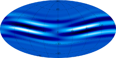
Figure 8: Surface map of the radial component of the magnetic field for an the case of an unstable A1 mode at ${{\rm Rm}=5000}$, ${S=35}$, and ${\beta=1}$. Light areas represent $b_{r}>0$, while dark areas are $b_{r}<0$.

According to Fig. 10, the Hall parameter and, therefore, the Hall effect vanish in deeper layers of a PNS’s envelope even for a moderate magnetic field of $10^{12}\ {\rm G}$. Only the outer layers with densities in the range of $\rho\sim 10^{10}$–$10^{11}\,{\rm g}\,\mbox{cm}^{-3}$ are characterised by the $R_{B}$ closer to unity.

Figure 9: Microphysical magnetic diffusivity as a function of density for a temperature of $10^{10}\ \mathrm{K}$.

Figure 10: The Hall parameter as a function of density for a temperature of $10^{10}\ \mathrm{K}$.

If the flow is laminar, $\mathrm{Rm}$ and $S$ are orders of magnitude larger than the examined parameter space in the stability map of Fig. 1, due to the low diffusivity (see Fig. 9). If, however, the flow becomes turbulent, the turbulent diffusivity is much larger (Naso et al. 2008), leading to much lower $\mathrm{Rm}$ (${\sim}10^{4}$, as noted by Kondić et al. 2011, and which are doable numerically), but still above the threshold for the onset of the Hall-MRI. An interesting feature of turbulent flows is that $S$ is close to unity for densities larger than or equal to $10^{13}\ {\rm g}\,\mbox{cm}^{-3}$. These regions will be purely SHI unstable, because the MRI is inhibited by diffusion.

Therefore, the Hall-MRI instabilities shall set in after the seed field of the progenitor is sufficiently amplified. They would probably first destabilise the outer regions, perhaps spreading inward provided that the fields in the interior become sufficiently strong (because the Hall parameter $R_{B}$ scales linearly with the magnetic field). If the flow is already turbulent for other reasons, even the pure SHI may be encountered in regions where the Lundquist number is small enough.

Given that we have shown the growth rates of the instability to depend on a general orientation of the magnetic field, those multipolar field components which have the opposite directions in different hemispheres, e.g. a quadrupole or a tilted dipole, will experience different growth. The fields with dominant negative orientation would be strongly restricted in their growth. This may have interesting implications for observable properties of the field, with one hemisphere having different field strength and patterns than the other.

The nonlinear effects related to this process are the self-coupling of the magnetic field through the quadratic Hall term, as well as the nonlinear nature of the flow/field interaction where Maxwell stresses redistribute the angular momentum in the fluid, braking the differential rotation on the time-scale comparable to the Alfvén time (shorter than any time-scale related to viscosity effects). These effects will need to be taken into account in order to obtain the estimates of the final amplitude and topology of the magnetic field available through the Hall-MRI. The proximity of the excitation thresholds of axisymmetric and non-axisymmetric modes is another interesting outcome of this paper; the nonlinear coupling of the modes may lead to different classes of surface field topologies with implications for the observability of neutron stars.

References

- Akiyama et al. (2003) Akiyama, S., Wheeler, J.C., Meier, D.L., Lichtenstadt, I.: 2003, ApJ 584, 954
- Ardeljan et al. (2005) Ardeljan, N.V., Bisnovatyi-Kogan, G.S., Moiseenko, S.G.: 2005, MNRAS 359, 333
- Balbus & Hawley (1991) Balbus, S.A., Hawley, J.F.: 1991, ApJ 376, 214
- Balbus & Hawley (1998) Balbus, S.A., Hawley, J.F.: 1998, Rev. of Modern Phys. 70, 1
- Balbus & Terquem (2001) Balbus, S.A., Terquem, C.: 2001, ApJ 552, 235
- Bejarano et al. (2011) Bejarano, C., Gómez, D.O., Brandenburg, A.: 2011, ApJ 737, 62
- Bonanno et al. (2006) Bonanno, A., Urpin, V., Belvedere, G.: 2006, A&A 451, 1049
- Burrows & Lattimer (1986) Burrows, A., Lattimer, J.M.: 1986, ApJ 307, 178
- Burrows et al. (2007) Burrows, A., Dessart, L., Livne, E., Ott, C.D., Murphy, J.: 2007, ApJ 664, 416
- Haensel et al. (2007) Haensel, P., Potekhin, A.Y., Yakovlev, D.G.: 2007, Neutron Stars 1: Equation of State and Structure, ASSL 326, Springer, New York
- Hollerbach (2000) Hollerbach, R.: 2000, Int. J. Numer. Meth. Fluids 32, 773
- Hollerbach & Rüdiger (2002) Hollerbach, R., Rüdiger, G.: 2002, MNRAS 337, 216
- Kitchatinov & Rüdiger (2010) Kitchatinov, L. L., Rüdiger, G.: 2010, A&A 513, L1
- Kondić et al. (2011) Kondić, T., Rüdiger, G., Hollerbach, R.: 2011, A&A 535, L2
- Kunz (2008) Kunz, M.W.: 2008, MNRAS 385, 1494
- Naso et al. (2008) Naso, L., Rezzolla, L., Bonanno, A., Paternò, L.: 2008, A&A 479, 167
- Obergaulinger et al. (2006) Obergaulinger, M., Aloy, M.A., Müller, E.: 2006, A&A 450, 1107
- Obergaulinger et al. (2009) Obergaulinger, M., Cerdá-Durán, P., Müller, E., Aloy, M.A.: 2009, A&A 498, 241
- Ott et al. (2006) Ott, C.D., Burrows, A., Thompson, T.A., Livne, E., Walder, R.: 2006, ApJS 164, 130
- Page et al. (2006) Page, D., Geppert, U., Weber, F.: 2006, Nucl. Phys. A 777, 497
- Potekhin (2008) Potekhin, A.Y.: 2008, Electron Conductivity of Stellar Plasmas, http://www.ioffe.ru/astro/conduct/index.html
- Rüdiger & Kitchatinov (2005) Rüdiger, G., Kitchatinov, L.L.: 2005, A&A 434, 629
- Shapiro & Teukolsky (1983) Shapiro, S.L., Teukolsky, S.A.: 1983, Black Holes, White Dwarfs, and Neutron Stars: The Physics of Compact Objects, Wiley-Interscience, New York
- Urpin & Rüdiger (2005) Urpin, V., Rüdiger, G.: 2005, A&A 437, 23
- Wardle (1999) Wardle, M.: 1999, MNRAS 307, 849