Measurability of the tidal polarizability of neutron stars in late-inspiral gravitational-wave signals

Abstract

The gravitational wave signal from a binary neutron star inspiral contains information on the nuclear equation of state. This information is contained in a combination of the tidal polarizability parameters of the two neutron stars and is clearest in the late inspiral, just before merger. We use the recently defined tidal extension of the effective one-body formalism to construct a controlled analytical description of the frequency-domain phasing of neutron star inspirals up to merger. Exploiting this analytical description we find that the tidal polarizability parameters of neutron stars can be measured by the advanced LIGO-Virgo detector network from gravitational wave signals having a reasonable signal-to-noise ratio of $\rho=16$. This measurability result seems to hold for all the nuclear equations of state leading to a maximum mass larger than $1.97M_{\odot}$. We also propose a promising new way of extracting information on the nuclear equation of state from a coherent analysis of an ensemble of gravitational wave observations of separate binary merger events.

I Introduction

Binary neutron star (BNS) inspirals are among the most promising sources for the advanced version of the ground based gravitational wave (GW) detector network LIGO-Virgo. BNS’s evolve under the influence of gravitational radiation reaction leading to a GW inspiral signal whose amplitude increases up to the merger, while its frequency also increases up to a merger frequency $f_{\rm merger}\lesssim 2000$ Hz. One of the goals of the observation of GW signals from BNS systems is to improve our knowledge about neutron star (NS) structure and the highly uncertain equation of state (EOS) of NS matter. Advanced LIGO is expected to be able to detect about 40 BNS merger events per year Abadie:2010cf with signal to noise ratio (SNR) $\rho\geq 8$. The question that we shall address here is whether such observations can allow us to learn something useful about the EOS of neutron star matter via the measurement of tidal polarizability parameters from the inspiral signal.

In Newtonian gravity the (quadrupolar) tidal polarizability of a body is usually measured by means of the dimensionless Love number $k_{2}$ such that $\mu_{2}=2/(3G)k_{2}R^{5}$, where $R$ denotes the radius of the NS, yields the ratio between the tidally induced quadrupole moment $Q_{ab}$ and the companion’s perturbing tidal gradient $G_{ab}=\partial_{ab}U$. The generalization of the concept of tidal Love number $k_{2}$ to strongly self-gravitating objects (NS or black holes) was discussed long ago by one of us as part of the theory of motion of compact bodies Damour:1983 . This work indicated how, by matching a quadrupolar deformed NS geometry treated à la Thorne and Campolattaro thorne:1967 , one could compute $k_{2}$ for a given neutron star EOS. Recently, an explicit, simple, way of doing this matching computation of $k_{2}$ has been obtained by Hinderer Hinderer:2007mb . The resulting numerical values for $k_{2}$ obtained in Ref. Hinderer:2007mb have then been used in a preliminary analysis of the measurability of tidal effects in BNS GW inspiral signals Flanagan:2007ix . However, this early work has been marred by a calculational error in Hinderer:2007mb leading to a substantial overestimate of the value of $k_{2}$. Later work Damour:2009vw ; Binnington:2009bb emphasized that $k_{2}$ is a strongly decreasing function of the NS compactness ${\cal C}\equiv GM/(c^{2}R)$, such that $k_{2}({\cal C})$ formally vanishes in the black hole limit ${\cal C}\to 1/2$, and generalized the computation of Love numbers so as to include gravito-magnetic tidal polarizability coefficients as well as higher multipolar contributions. Recently Hinderer:2009ca the tidal polarization parameter $\mu_{2}$ was computed for a wide range of EOS. Moreover, the question of discriminating between NS EOSs via GW observations with the advanced LIGO-Virgo detector network, using the early part (frequencies $f<450$ Hz) of the inspiral signal, has been discussed and answered in the negative in Hinderer:2009ca : only if one has a GW signal with very high SNR $\rho=35$, and if the actual EOS of NS matter is unusually stiff, can one start distinguishing (at the $68\%$ confidence level) the early-inspiral tidal signal from the noise.

The reason why Refs. Flanagan:2007ix ; Hinderer:2009ca performed a conservative data analysis based only on the early inspiral GW signal, $f<450$ Hz, was that their analysis was based on using a purely post-Newtonian (PN) expanded description of the phasing, without having any way of controlling the validity of this description for frequencies above 450 Hz. More precisely, they use a TaylorF2-type Damour:2000zb description of the frequency-domain GW phase of the form $\Psi(f)=\Psi^{0}_{\rm PN}(f)+\Psi^{T}_{\rm N}(f)$, with a point-mass phasing $\Psi^{0}_{\rm PN}(f)$ treated at 3.5PN accuracy Damour:2000zb and with a tidal phasing $\Psi^{T}_{\rm N}(f)$ treated at leading, Newtonian order Flanagan:2007ix .

Recently, a new, improved description of the dynamics, waveform and phasing of compact binary systems has been developed based on the effective one body (EOB) formalism Buonanno:1998gg ; Buonanno:2000ef ; Damour:2000we ; Damour:2001tu ; Damour:2008gu ; Damour:2009ic . In particular, the way to extend the EOB formalism so as to include tidal effects has been presented in Damour:2009wj . Let us recall that the EOB formalism is an analytical framework which combines several different theoretical results and approaches, and, in particular, contains resummed versions of the usual PN-expanded results. Such a framework has proven to be a powerful tool for constructing analytic waveforms that agree with numerical simulations. In the binary black hole case, EOB waveforms are in agreement with high-accuracy numerical waveforms at the remarkable level of 0.01 rad up to merger Damour:2009kr ; Pan:2009wj ; Pan:2011gk . In addition, the tidal-EOB formalism of Damour:2009wj has been successfully compared to state-of-the-art numerical simulations of BNS systems Baiotti:2010xh ; Baiotti:2011am . This comparison showed that the tidal-EOB formalism could reproduce the numerical phasing essentially up to merger within numerical uncertainties.

This successful comparison (together with recent analytical progress Bini:2012gu in the computation of the EOB tidal interaction potential) motivates us here to use the tidal-EOB formalism as a way to define a controlled analytical description of the phasing of tidally interacting BNS systems up to merger. More precisely, we will show below that the tidal contribution $\Psi^{T}_{\rm EOB}(f)$ to the Fourier domain phase predicted by the tidal-EOB approach can be represented (within less than 0.3 rad) by a certain (PN-type) analytical expression up to merger. This will allow us to perform a data analysis using the full tidal phasing signal up to merger, while keeping the convenience of having an explicit analytical representation of the tidal phasing (instead of the well-defined, but more indirect, full EOB description of tidally interacting BNS systems). Using such a EOB-controlled description of the tidal phasing up to merger, we will show (see Fig. 4 below) that the EOS-dependent tidal polarizability parameters $G\mu_{2}$ of NSs can be measured, at the $95\%$ confidence level, with the advanced LIGO-Virgo detector network using GW signals with reasonable SNRs ($\rho=16$) for all EOS in the sample we shall consider (only restricted by the observational constraint of yielding a maximum mass larger than $1.97M_{\odot}$ Demorest:2010bx ). In addition we shall propose a new way of extracting EOS-dependent information from a coherent analysis of a collection of GW observations of separate BNS merger events, which promises a large increase in measurement accuracy.

In this paper we will focus on BNS systems, but the formalim we present can be used as it is for discussing the measurability of tidal parameters in mixed BH-NS binary systems. This would allow one to go beyond the recent works Pannarale:2011pk ; Lackey:2011vz dealing with some aspects of the measurability of tidal polarizability coefficients from mixed binary systems.

The paper is organized as follows: in Sec. II we will review the main elements of the tidal-EOB formalism and present the analytic tidal phasing model in the frequency domain that we will use in estimating the measurability of $\mu_{2}$. The theoretical aspects of our measurability analysis are given in Sec. III. The numerical results for the measurability of $\mu_{2}$ are presented in Sec. IV, while concluding remarks are gathered in Sec. V. The paper is completed by two Appendices. In Appendix A we extend and complete the review of the tidal-EOB formalism of Sec. II, giving in particular the explicit analytical expressions for the tidal corrections to the EOB waveform. Finally, Appendix B collects the PN-expanded formulas for the tidal phasing for a general relativistic binary that are used in the main text. When convenient, we use geometrized units with $G=c=1$.

II Analytical tidal phasing models in the frequency domain

The main aim of the present paper will be to estimate the measurability of tidal parameters by making use of the full BNS inspiral signal, including the late-inspiral part just before merger, where tidal effects are strongest. We will do so by taking advantage of the recent development of an analytical model which can accurately describe the full inspiral signal up to merger. Indeed, in Refs. Baiotti:2010xh ; Baiotti:2011am state-of-the-art numerical simulations of inspiralling BNS systems were compared to several analytical models. It was found that the EOB model (in its tidally extended version as defined in Damour:2009wj ) was able to match the numerical results up to merger. The EOB model (dynamics and waveform) is originally defined in the time domain. For the data-analysis purpose of the present paper it will be convenient to have in hands an analytic representation of the waveform in the frequency domain. The derivation of such an analytic frequency-domain phasing model will be the topic of the present Section.

II.1 Tidal effects in EOB dynamics

Let us recall that the EOB formalism Buonanno:1998gg ; Buonanno:2000ef ; Damour:2001tu consists of three main elements: (i) a resummed Hamiltonian describing the conservative dynamics; (ii) a radiation-reaction force computed from the instantaneous angular momentum loss; (iii) a resummed waveform.

For a nonspinning binary black hole (BBH) system of masses $M_{A}$, $M_{B}$ the EOB Hamiltonian is given by

$$H_{\rm EOB}(r,p_{r_{*}},p_{\varphi})\equiv Mc^{2}\sqrt{1+2\nu(\hat{H}_{\rm eff}-1)}\ ,$$ (1)

where

$$\hat{H}_{\rm eff}\equiv\sqrt{p_{r_{*}}^{2}+A(r)\left(1+\frac{p_{\varphi}^{2}}{r^{2}}+z_{3}\,\frac{p_{r_{*}}^{4}}{r^{2}}\right)}\,.$$ (2)

Here $M\equiv M_{A}+M_{B}$ is the total mass, $\nu\equiv M_{A}\,M_{B}/(M_{A}+M_{B})^{2}$ is the symmetric mass ratio, and $z_{3}\equiv 2\nu(4-3\nu)$. In addition, we are using rescaled dimensionless (effective) variables, namely $r\equiv r_{AB}c^{2}/GM$ and $p_{\varphi}\equiv P_{\varphi}c/(GM_{A}M_{B})$, and $p_{r_{*}}$ is canonically conjugated to a “tortoise” modification of $r$ Damour:2009ic . The crucial input entering this Hamiltonian is the “radial potential” $A(r)$, whose leading-order approximation is $A(r)\approx 1-2/r+\dots\equiv 1-2GM/(c^{2}r_{AB})+\dots$

The proposal of Ref. Damour:2009wj for including dynamical tidal effects in the conservative part of the dynamics consists in using a tidally-augmented radial potential of the form

$$A(r)=A^{0}(r)+A^{\rm tidal}(r).$$ (3)

where $A^{0}(r)$ is the point-mass potential defined in Eq. (88) of Appendix A, while $A^{\rm tidal}(r)$ is a supplementary “tidal contribution” describing the tidal interaction potential. In terms of the dimensionless gravitational potential $u\equiv GM/(c^{2}r_{AB})\equiv 1/r$ it reads

$$A^{\rm tidal}=\sum_{\ell\geq 2}-\kappa_{\ell}^{T}u^{2\ell+2}\hat{A}^{\rm tidal}_{\ell}(u).$$ (4)

Here the term $\kappa^{T}_{\ell}u^{2\ell+2}$ represents the multipolar tidal interaction of degree $\ell$, taken at Newtonian order in a PN expansion. The dimensionless EOB tidal parameter $\kappa_{\ell}^{T}$ entering Eq. (4) is related to the tidal polarizability coefficients $G\mu_{\ell}^{A,B}$ of each neutron star as Damour:2009wj

$${\kappa}_{\ell}^{T} \equiv\kappa^{A}_{\ell}+\kappa_{\ell}^{B}$$ (5)

where

$$\kappa_{\ell}^{A}\equiv\left(2\ell-1\right)!!\dfrac{X_{B}}{X_{A}}\dfrac{G\mu_{\ell}^{A}}{(GM/c^{2})^{2\ell+1}}.$$ (6)

where we recall that $M=M_{A}+M_{B}$ denotes the total mass of the binary and $X_{A}\equiv M_{A}/M$. The tidal polarizability coefficient $G\mu_{\ell}^{A}$ has the dimension $[\rm length]^{2\ell+1}$. It measures the ratio between the $\ell$-th multipole moment induced in body $A$ and the external tidal gradient felt by body $A$. Among these multipolar tidal polarizability coefficients, the dominant one is the quadrupolar, $\ell=2$, one, $G\mu_{2}^{A}$. [Note that $\mu_{2}$ is denoted by $\lambda$ in Refs. Flanagan:2007ix ; Hinderer:2009ca ; Pannarale:2011pk ]. In addition, if $R_{A}$ denotes the radius of body $A$, $G\mu_{\ell}^{A}$ is related to the corresponding dimensionless Love number $k_{\ell}^{A}$ by

$$(2\ell-1)!!\,G\mu^{A}_{\ell}=2k_{\ell}^{A}\,R_{A}^{2\ell+1},$$ (7)

so that

$$\kappa_{\ell}^{A}=2k_{\ell}^{A}\dfrac{X_{B}}{X_{A}}\left(\dfrac{R_{A}}{G(M_{A}+M_{B})/c^{2}}\right)^{2\ell+1}.$$ (8)

The additional factor $\hat{A}^{\rm tidal}_{\ell}(u)$ in Eq. (4) represents the effect of distance-dependent, higher-order relativistic contributions to the dynamical tidal interactions: 1PN, i.e. first order in $u$, 2PN, i.e. of order $u^{2}$, etc. Here we will use the following “Taylor-expanded” form of $\hat{A}^{\rm tidal}_{\ell}$

$$\hat{A}^{\rm tidal}_{\ell}(u)=1+\bar{\alpha}_{1}^{(\ell)}u+\bar{\alpha}_{2}^{(\ell)}u^{2}\ ,$$ (9)

where $\bar{\alpha}_{n}^{(\ell)}$ are functions of $M_{A}$, ${\cal C}_{A}$, and $k_{\ell}^{A}$ for a general binary and are defined as (see Eq. (37) of Damour:2009wj )

$$\bar{\alpha}_{n}^{(\ell)}\equiv\dfrac{\kappa_{\ell}^{A}\alpha^{A(\ell)}_{n}+\kappa_{\ell}^{B}\alpha^{B(\ell)}_{n}}{\kappa_{\ell}^{A}+\kappa_{\ell}^{B}},$$ (10)

where $\alpha^{A(\ell)}_{n}$ is the coefficient of the the $n$PN fractional correction to the tidal interaction potential of body $A$. (see Sec. IIIC of Damour:2009wj ). The individual dimensionless coefficient $\alpha_{n}^{A(\ell)}$ is a function of the dimensionless ratio $X_{A}\equiv M_{A}/M$. [Note that $X_{B}\equiv M_{B}/M=1-X_{A}$]. The analytical expression of the first post-Newtonian, quadrupolar ($\ell=2$) coefficient $\alpha_{1}^{A(2)}$ has been reported in Damour:2009wj (and then confirmed in Vines:2010ca ) and reads

$$\alpha_{1}^{A(2)}=\dfrac{5}{2}X_{A}.$$ (11)

Recently, Ref. Bini:2012gu has succeeded in computing the first post-Newtonian octupolar ($\ell=3$) coefficient $\alpha_{1}^{A(3)}$, as well as the second post-Newtonian quadrupolar ($\ell=2$) and octupolar ($\ell=3$) coefficients $\alpha_{2}^{A(\ell)}$. The most relevant 2PN quadrupolar coefficient reads

$$\alpha_{2}^{A(2)}=\dfrac{337}{28}X_{A}^{2}+\dfrac{1}{8}X_{A}+3.$$ (12)

In the equal-mass case, $X_{A}=1/2$, the values of these coefficients are $\alpha_{1}^{A(2)}=\bar{\alpha}^{(2)}_{1}=5/4=1.25$ and $\alpha_{2}^{A(2)}=\bar{\alpha}_{2}^{(2)}=85/14\approx 6.071429$. A recent comparison Baiotti:2010xh ; Baiotti:2011am between EOB predictions and BNS numerical simulations concluded that $\bar{\alpha}^{(2)}_{2}\lesssim 40$. In the following, we shall restrict ourselves to considering only tidal quadrupolar contributions, i.e. we will take only the $\ell=2$ value in Eqs. (4) and (9). It is shown in Section A.2 of Appendix A that the effect of higher-$\ell$ tidal corrections is small. It will be neglected in our analysis.

II.2 EOB waveform and its stationary phase approximation

When considering tidally interacting binary systems, one needs to augment the point-mass waveform $h_{{\ell m}}^{0}$ by tidal contributions. Similarly to the additive tidal modification (4) of the $A$ potential, we will here consider an additive modification of the waveform, having the structure

$$h_{{\ell m}}=h_{{\ell m}}^{0}+h_{\ell m}^{\rm tidal}.$$ (13)

See Appendix A for the explicit expressions of $h_{{\ell m}}^{0}$ and $h_{\ell m}^{\rm tidal}$. In turn, this tidally modified waveform defines a corresponding tidally modified radiation reaction force ${\cal F}_{\varphi}$ through its instantaneous angular momentum loss.

The radiation-driven EOB dynamics defined by $H_{\rm EOB}(A)$ and ${\cal F}_{\varphi}$ (where both $A$ and ${\cal F}_{\varphi}$ are tidally modified) allows us to compute a time-domain multipolar GW signal $h_{\ell m}(t)=A_{{\ell m}}(t)e^{-{\rm i}\phi_{\ell m}(t)}$. Following Refs. Baiotti:2010xh ; Baiotti:2011am , we characterize the (time-domain) phasing of the quadrupolar waveform $h_{22}(t)$ by means of the following function of the instantaneous quadrupolar GW frequency $\omega=\omega(t)\equiv d\phi/dt$ [where $\phi(t)\equiv\phi_{22}(t)$]

$$Q_{\omega}(\omega)\equiv\dfrac{d\phi(t)}{d\ln\omega(t)}\equiv\dfrac{[\omega(t)]^{2}}{\dot{\omega}(t)}.$$ (14)

In the stationary phase approximation (SPA), the phase $\Psi(f)$ of the frequency-domain waveform $\tilde{h}(f)$, i.e. the phase of the Fourier transform of the time-domain (quadrupolar) waveform,

$$\tilde{h}_{22}(f)\equiv\tilde{A}(f)e^{-{\rm i}\Psi(f)},$$ (15)

is simply the Legendre transform of the quadrupolar time-domain phase $\phi(t)$, namely

$$\Psi_{\rm SPA}(f)=2\pi ft_{f}-\phi(t_{f})-\dfrac{\pi}{4},$$ (16)

where $t_{f}$ is the saddle point of the Fourier transform, i.e. the solution of the equation $\omega(t_{f})=2\pi f$. Differentiating Eq. (16) twice with respect to $f$ leads to the following link between $\Psi_{\rm SPA}(f)$ and the function $Q_{\omega}(\omega)$

$$\dfrac{d^{2}\Psi_{\rm SPA}(\omega_{f})}{d\omega_{f}^{2}}=\dfrac{Q_{\omega}(\omega_{f})}{\omega_{f}^{2}},$$ (17)

where $\omega_{f}$ now denotes the Fourier domain circular frequency $\omega_{f}\equiv 2\pi f$. Below we will simply denote the Fourier domain frequency $\omega_{f}$ as $\omega$ without bothering to distinguish it from the time-domain $\omega(t)$.

In the following we shall decompose the result (17) in its point-mass and tidal parts, thereby relating the “tidal part” of the Fourier-domain phase $\Psi_{\rm SPA}(f)$ to the “tidal part” of $Q_{\omega}(\omega)$. On the one hand, the tidal part, say $Q_{\omega}^{T}(\omega)$, of $Q_{\omega}(\omega)$ is computed as

$$Q_{\omega}^{T}(\omega)=Q_{\omega}(\omega)-Q_{\omega}^{0}(\omega),$$ (18)

where $Q_{\omega}^{0}(\omega)$ is the outcome of a point-mass EOB simulation, i.e., one without tidal effects in both the dynamics and the waveform. Then, the corresponding tidal part,

$$\Psi^{T}_{\rm EOB}(\omega)=\Psi_{\rm EOB}(\omega)-\Psi^{0}_{\rm EOB}(\omega),$$ (19)

of the Fourier-domain EOB phase satisfies, within the SPA approximation, the relation

$$\dfrac{d^{2}\Psi^{T}_{\rm EOB_{SPA}}(\omega)}{d\omega^{2}}=\dfrac{Q^{T}_{\omega}(\omega)}{\omega^{2}}.$$ (20)

Let us emphasize that we expect the SPA approximation to the phasing to remain accurate up to the merger. Indeed the small parameter that controls the validity of the SPA is essentially $\epsilon_{\rm adiab}=\dot{\omega}/\omega^{2}\equiv 1/Q_{\omega}$. For instance, Ref. Damour:2000gg , Eqs. (3.9)-(3.10), has computed the next contribution beyond the leading SPA and found that it introduces a dephasing $\delta\Psi$ which, in the case of Newtonian chirps, is equal to $\delta\Psi=(23/24)\times(2/9)\times 1/Q_{\omega}$. The quantity $Q_{\omega}$ is very large during early inspiral and decreases towards the merger. Looking at the value of the full $Q_{\omega}=Q_{\omega}^{0}+Q_{\omega}^{T}$ in the exact EOB description of tidally interacting BNS systems, we have checked that the (equal-mass) value of $Q_{\omega}(\omega)$ for $\omega=\omega^{\rm contact}$ (where $\omega^{\rm contact}$ is the EOB approximation to the merger frequency, see below) remains larger than about 20 for realistic compactnesses (${\cal C}=0.14-0.18$). Though this value is reduced (by $\sim 10$) from the corresponding point-mass value $Q_{\omega}^{0}(\omega_{\rm contact})$, it is still comfortably large compared to $1$, so that one can expect the phasing error linked to the use of the SPA to be a small fraction of a radian.

II.3 PN-expansion of the EOB tidal phasing

In Sec. IV below we shall estimate the measurability of the tidal parameter $\kappa_{2}^{T}$ by computing the Fisher matrix ${\bf F}$ corresponding to the simultaneous measurement of a tidal parameter, say $\lambda_{T}\propto\kappa_{2}^{T}$, with several other, non tidal, parameters, say $\lambda_{a}$, $a=1,\dots,n$. Though, in principle we could numerically compute the relevant Fisher matrix ${\bf F}$ by evaluating the numerical derivatives of the full, Fourier domain, EOB waveform $\tilde{h}_{\rm EOB}(f;\,\lambda_{T},\lambda_{a})$ with respect to all the parameters $(\lambda_{T},\lambda_{a})$, it will be convenient to estimate ${\bf F}$ by replacing the numerically computed $\tilde{h}_{\rm EOB}(f;\,\lambda_{T},\lambda_{a})$ (which involves computing the numerical Fourier transform of a numerically generated time-domain EOB waveform $h_{\rm EOB}(t;\,\lambda_{T},\lambda_{a})$) by some sufficiently accurate analytic approximation. We will do so by combining several approximations, the validity of which we shall control. The first approximation we shall use is the SPA, which we have discussed in the previous section. The second approximation will consist in using post-Newtonian expansions to derive adequately accurate expressions of the two parts of the Fourier domain phase

$$\Psi(f)=\Psi^{0}(f;\,\lambda_{a})+\Psi^{T}(f;\,\lambda_{T},\lambda_{a}).$$ (21)

In this section we study how many terms in the PN expansion of the tidal phase $\Psi^{T}(f;\,\lambda_{T},\lambda_{a})$ we must retain to obtain an approximation to $\Psi^{T}(f)$ which remains reasonably close to the EOB prediction up to merger. From Eq. (19) we see (in the SPA) that to answer this question we need to compare the PN-expansion of the tidal part of $Q_{\omega}^{T}(\omega)$ of $Q_{\omega}(\omega)$ to the “exact” value of $Q_{\omega}^{T}(\omega)$ defined by the EOB model. During most of the inspiral , not only is the phase evolution quasi-adiabatic, i.e. $Q_{\omega}\gg 1$, as already discussed above, but the dynamical evolution can also be well approximated by an adiabatic quasi-circular inspiral. In the latter approximation, the function $Q_{\omega}=\omega^{2}/\dot{\omega}$ is obtained by writing the balance equation between the instantaneous energy flux $F$ at infinity and the adiabatic evolution of the energy of the system (i.e., the Hamiltonian, $H(\omega)$) expressed as a function of the instantaneous GW frequency $\omega=2\Omega$ (where $\Omega$ is the orbital frequency). This yields $-F=dH/dt=\left(dH/d\omega\right)\dot{\omega}$, from which one obtains

$$Q_{\omega}^{\rm adiab}(\omega)=-\omega^{2}\dfrac{dH(\omega)/d\omega}{F(\omega)}.$$ (22)

Reexpressing this result in terms of the dimensionless rescaled angular momentum $j\equiv J/(G\mu M)$, the Newton normalized energy flux $\hat{F}\equiv F/F^{\rm Newton}\equiv{\cal F}_{\varphi}/{\cal F}^{\rm Newton}_{\varphi}$, and replacing the independent variable $\omega$ by the usual, dimensionless PN ordering parameter

$$x\equiv\left(\dfrac{1}{2}\dfrac{GM\omega}{c^{3}}\right)^{2/3}\equiv\left(\dfrac{\pi GMf}{c^{3}}\right)^{2/3}$$ (23)

leads to an expression of the form

$$Q^{\rm adiab}_{\omega}(x;\,\nu,\lambda_{T})=\dfrac{5}{48\nu}x^{-5/2}b(x;\,\nu,\lambda_{T})$$ (24)

where the function $b(x;\,\nu,\lambda_{T})$, defined as

$$b(x;\,\nu,\lambda_{T})=-2x^{3/2}\dfrac{\partial_{x}j(x;\,\nu,\lambda_{T})}{\hat{F}(x;\,\nu,\lambda_{T})},$$ (25)

is simply equal to 1 in the Newtonian approximation. More precisely, it starts as

$$b(x;\,\nu,\lambda_{T})=1+\dfrac{1}{336}\left(743+924\nu\right)x-4\pi x^{3/2}+{\cal O}(x^{2}).$$ (26)

Starting from the adiabatic EOB dynamics, the function $j(x)$ is obtained by eliminating $u=1/r$ between the EOB expression $j^{2}(u)=-A^{\prime}(u)/(u^{2}A(u))^{\prime}$ (obtained by minimizing the effective potential for circular orbits $A(r)(1+j^{2}/r^{2})$) and the expression of $\Omega$ in terms of $u$ obtained from the Hamilton equation $\Omega=\partial H/\partial J$.[See Sec. III and IV of Ref. Damour:2009wj and Appendix A for more details about the EOB circular dynamics]. On the other hand, the function $\hat{F}(x)$ is obtained by as a sum of various resummed circular multipolar waveforms $h_{\ell m}(x)$ of Ref. Damour:2008gu .

In the following, we shall replace the (EOB-resummed) adiabatic approximation $Q_{\omega}^{\rm adiabatic}$, Eq. (22), to $Q_{\omega}^{\rm EOB}$, by a sufficiently accurate PN expansion of $Q_{\omega}^{\rm adiabatic}$. This is to avoid an inaccurate feature of $Q_{\omega}^{\rm adiabatic}$ during the late inspiral. From Eq. (22) we see that $Q_{\omega}^{\rm adiabatic}(\omega)$ is proportional to the derivative $dH(\omega)/d\omega$ which, by construction, vanishes at the Last Stable Orbit (LSO), where the circular energy $H(\omega)$ reaches a minimum. By contrast, the exact $Q_{\omega}^{\rm EOB}$ does not vanish at the LSO, nor the PN expanded version of $Q_{\omega}^{\rm EOB}$ that we shall use. The frequency corresponding to the tidal-EOB defined LSO happens to be quite close to the contact frequency. Using $Q_{\omega}^{\rm adiabatic}$ up to contact might then introduce inaccuracies in the phasing just before merger. Our use below of a suitable PN-expanded representation of $Q_{\omega}$ avoids this source of uncertainty and maintains consistency with the SPA by allowing the value of $Q_{\omega}$ at contact to remain of order 20 for all cases considered.

Current analytical knowledge that has been incorporated in the EOB description of tidal effects Baiotti:2010xh ; Baiotti:2011am allows us to compute the tidal part $Q_{\omega}^{T}(\omega)$ of $Q_{\omega}(\omega)$ and therefore, using Eq. (20), the tidal part $\Psi^{T}(\omega)$ of the Fourier domain phase $\Psi(\omega)$ beyond the 1PN accuracy obtained in Ref. Vines:2011ud . First, the fact that the EOB formalism naturally accomodates the inclusion of tail effects in the waveform allows us to obtain a PN-expanded tidal phasing model that is analytically complete up to 1.5PN order. [In addition, the EOB formalism already contains the next order tail effects at 2.5PN order]. Second, the EOB approach is designed in a way which makes it easy to complete it beyond current analytical knowledge by using effective field theory methods. In particular, Ref. Bini:2012gu recently computed the 2PN tidal contributions to the EOB radial potential $A(u)$, i.e. the coefficient $\bar{\alpha}_{2}$ of $u^{2}$ in Eq. (9) (see Eq. (94)). As mentioned in Ref. Bini:2012gu , a straightforward extension of the method used to derive the 2PN tidal contribution to $A(u)$ can allow one to derive the 2PN tidal contribution to the waveform. However this calculation has not yet been completed. Waiting for this result, we shall here use the natural flexibility of the EOB formalism, to parametrize the 2PN tidal corrections to the multipolar waveform by means of some parameters that we will call $\beta_{n}^{\ell m}$. Let us recall that in order to obtain $Q_{\omega}^{T}$ at, say, the fractional 2.5PN accuracy, the energy flux $F$ must be computed by retaining all the $\ell=2$ and $\ell=3$ multipolar contributions to the waveform. Then, to obtain the flux to 2.5PN accuracy we need the quadrupolar $\ell=m=2$ waveform (stripped of its tail factor) to 2PN fractional accuracy, and the odd-parity $\ell=2$, $m=1$ and $\ell=m=3$ and $\ell=3$, $m=1$ even-parity waveforms at 1PN fractional accuracy. Following Refs. Damour:2009wj ; Baiotti:2011am , we shall parametrize such higher-PN tidal corrections to the waveform along the following model

$$h_{\ell m}^{\rm tidal}=h_{\ell m}^{A\,{\rm tidal}}+h_{\ell m}^{B\,{\rm tidal}},$$ (27)

with

$$h_{\ell m}^{A\,{\rm tidal}}=h_{\ell m}^{A\,{\rm tidal_{Newt}}}\left(1+\beta^{{\ell m}}_{1}(X_{A})x+\beta^{{\ell m}}_{2}(X_{A})x^{2}+\dots\right).$$ (28)

For the time being, the only such PN fractional tidal waveform correction which is known is $\beta_{1}^{22}(X_{A})$. Using the 1PN-accurate results of Ref. Vines:2011ud one can indeed derive the following explicit analytical expression

$$\beta_{1}^{22}(X_{A})=\dfrac{-202+560X_{A}-340X_{A}^{2}+45X_{A}^{3}}{42(3-2X_{A})}.$$ (29)

However, at 2.5PN, the final result depends on several other higher-corrections, namely $\beta_{2}^{22}(X_{A})$, $\beta_{1}^{21}(X_{A})$, $\beta_{1}^{33}(X_{A})$ and $\beta_{1}^{31}(X_{A})$ , that account respectively for 2PN fractional tidal corrections to the $\ell=m=2$ multipole and for 1PN fractional tidal corrections to the $\ell=2$, $m=1$ and $\ell=3$, $m=1$ and $m=3$ subdominant multipoles. In Appendix B we present the explicit expressions for $Q_{\omega}^{T}$ and $\Psi^{T}$ at 2.5PN accuracy for the general case of unequal mass binary systems. In the text below we shall specify those general formulas to the particular, but physically most relevant, case of equal-mass neutron star binaries (having therefore equal-compactnesses and equal tidal parameters).

In the equal-mass case, because of symmetry reasons, the only higher-order tidal waveform parameter that contributes to the phasing is $\beta_{2}^{22}$. We then arrive at the following explicit expression for the 2.5PN accurate tidal contribution to $Q_{\omega}$

$$Q_{\omega}^{T}(x) =-{\kappa_{2}^{T}}\dfrac{65}{6}x^{5/2}\bigg{[}1+\dfrac{4361}{624}x-4\pi x^{3/2}$$

$$+\left(\dfrac{4614761}{122304}+\dfrac{4}{3}\bar{\alpha}_{2}^{(2)}+\dfrac{4}{13}\beta_{2}^{22}\right)x^{2}-\dfrac{4283}{156}\pi x^{5/2}\bigg{]},$$ (30)

where we recall that $\bar{\alpha}^{(2)}_{22}=\alpha_{2}^{A(2)}(X_{A}=1/2)=85/14$ and where $\beta_{2}^{22}$ denotes the value of the (unknown) function $\beta^{2}_{22}(X_{A})$ for $X_{A}=1/2$. Using Eq. (20), the corresponding 2.5PN accurate tidal phase of the Fourier transform of the GW signal reads (in the SPA)

$$\Psi^{T}_{\rm 2.5PN}(x) =-{\kappa_{2}^{T}}\dfrac{39}{4}x^{5/2}\bigg{\{}1+\dfrac{3115}{1248}x-\pi x^{3/2}$$

$$+\left(\dfrac{23073805}{3302208}+\dfrac{20}{81}\bar{\alpha}_{2}^{(2)}+\dfrac{20}{351}\beta_{2}^{22}\right)x^{2}$$

$$-\dfrac{4283}{1092}\pi x^{5/2}\bigg{\}}.$$ (31)

Such an explicit representation of a Fourier domain phase as a polynomial in $x(f)\propto f^{2/3}$ is usually called TaylorF2 Damour:2000zb . The 2.5PN TaylorF2 formula (II.3) improves the 1PN result of Ref. Vines:2011ud in that: (i) tail effects are included up to 2.5PN order; (ii) a large part of the 2PN term is explicitly computed, although it still depends on the yet uncalculated quantity $\beta_{2}^{22}$ (2PN tidal correction to the waveform). Note that at leading, Newtonian, order, Eq. (II.3) predicts that the (equal-mass) tidal dephasing at contact, i.e. for $x_{\rm contact}={\cal C}_{A}={\cal C}_{B}$ (see Eq. (36)) is of order

$$\Psi_{\rm Newt-equal-mass}^{\rm contact}=-\dfrac{39}{32}\dfrac{k_{2}^{A}}{{\cal C}_{A}^{5/2}},$$ (32)

which, for the typical values $k_{2}=0.08$ and ${\cal C}=1/6$, yields $-8.6$ rad. With the further amplification of PN effects discussed below this means that the tidal dephasing at contact is of order $-10$ rad (see Fig. 1).

Let us now indicate why we expect that the contribution to the tidal phase coming from $\beta_{2}^{22}$ is likely to be numerically subdominant compared to the currently known terms. Let us first note that at leading, Newtonian order the overall coefficient $(39/4)\kappa_{2}^{T}$ in the tidal phase Eq. (II.3), is, in view of Eq. (22), the sum of a tidal contribution from the Hamiltonian $H$ and a tidal contribution from the energy flux $F$. More precisely, one finds that

$$\dfrac{39}{4}=\dfrac{3}{4}\left(9_{H}+4_{F}\right)$$ (33)

where the indices indicate the origin ($H$ or $F$) of the contribution. Already at this leading-order level, one notices that the contribution from the energy flux is subdominant (by a factor 2.25) with respect to the contribution from the Hamiltonian, i.e. from the radial potential $A(u)$. When pursuing this analysis at the 1PN level and considering the fractional PN modification of the tidal phase $\hat{\Psi}^{T}_{\rm 2.5PN}\equiv\Psi^{T}_{\rm 2.5PN}/\Psi^{T}_{\rm Newt}\equiv 1+{\cal O}(x)$ in Eq. (II.3) one finds (still for the equal-mass case)

$$\hat{\Psi}^{T}_{\rm 1PN} =1+\left(\dfrac{125795}{61152}+\dfrac{55}{156}\bar{\alpha}_{1}^{(2)}+\dfrac{10}{91}\beta_{1}^{22}\right)x$$

$$\approx 1+\left(2.05709+0.35256\bar{\alpha}_{1}^{(2)}+0.10989\beta_{1}^{22}\right)x,$$ (34)

where we decomposed the 1PN fractional contribution into three parts: i) one coming from the leading order tidal terms in $H$ and $F$; ii) one coming from the 1PN tidal correction to $H$ (term $\propto\bar{\alpha}_{1}^{(2)}$); and (iii) one coming from the 1PN tidal correction to the quadrupolar waveform (and flux, term $\propto\beta_{1}^{22}$). In the equal-mass case one has $\bar{\alpha}_{1}^{(2)}=5/4=1.25$ and $\beta_{1}^{22}=-11/672\approx-0.0164$. As a consequence of these numerical values, we see that: a) the coefficient of $\beta_{1}^{22}$ is smaller by a factor 3.2 than the coefficient of $\bar{\alpha}_{1}^{(2)}$; b) in addition, as the numerical value of $\beta_{1}^{22}$ is $\approx-0.0164$, its contribution to the total 1PN fractional coefficient is $0.10989\times 0.0164/2.05709\approx 8.8\times 10^{-4}$ times smaller than the first term 2.057 and $7.2\times 10^{-4}$ times smaller than the sum of the first two contributions. Performing a similar analysis at the 2.5PN level (now inserting the known numerical values of $\bar{\alpha}_{1}^{(2)}$ and $\beta_{1}^{22}$) yields

$$\hat{\Psi}^{T}_{\rm 2.5PN} \approx 1+2.50x-\pi x^{3/2}$$ (35)

$$+(6.99+0.25\bar{\alpha}_{2}^{(2)}+0.057\beta_{2}^{22})x^{2}-3.92\pi x^{5/2}.$$

Again we see that the contribution from $\beta_{2}^{22}$ is likely to be subdominant. Indeed, not only is the coefficient of $\beta_{2}^{22}$ 4.3 times smaller than the one of $\bar{\alpha}_{2}^{(2)}$, but it is also about 149 times smaller than the known 2PN coefficient $6.99+0.25\bar{\alpha}_{2}^{(2)}\approx 8.51$. Independently of these numerical arguments, let us note that, as already mentioned above, an important feature of the adiabatic approximation to the function $Q_{\omega}(\omega)$ is that it vanishes at the adiabatic LSO. Since tidal effects strongly influence the LSO location (see Ref. Damour:2009wj ) this indicates that tidal corrections to the Hamiltonian (i.e., to $A(u)$) have a dominant influence on the shape of the $Q_{\omega}(\omega)$ function below the LSO frequency and thereby on the tidal corrections to $\Psi^{T}(\omega)$. In view of these arguments, in the following we will neglect the effect of $\beta_{2}^{22}$ both in the exact EOB phase and its 2.5PN approximant, $\Psi^{T}_{\rm 2.5PN}(\omega)$. We will then work with Eq. (II.3) with $\beta^{22}_{2}=0$ (but $\bar{\alpha}_{2}^{(2)}=85/14\approx 6$) as a numerically acceptable approximation to the 2.5PN tidal phase.

II.4 Accuracy of PN-expanded representations of the EOB phasing

Let us now study to what extent the “exact” EOB tidal phasing $\Psi_{\rm EOB_{SPA}}^{T}$ obtained by integrating Eq. (20) with the exact (time-domain) $Q_{\omega}(\omega)$ defined by Eq. (14) on the right hand side, can be represented by various PN expansions.

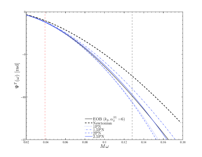
Figure 1: Successive PN approximants to the (SPA) tidal contribution to the EOB phase as function of the $\ell=m=2$ GW frequency. The leftmost vertical line indicates 450 Hz for a $1.4M_{\odot}+1.4M_{\odot}$ BNS system. The rightmost vertical line indicates the contact frequency that is taken as a fiducial analytical definition of the moment of merger. The plot refers to a ${\cal C}=0.16$, $\gamma=2$ polytropic model.

Fig. 1 illustrates the performance of Eq. (II.3) (considered at different orders of truncation) in reproducing $\Psi_{\rm EOB_{SPA}}^{T}$. The figure refers to an equal-mass binary, with $\gamma=2$ polytropic EOS $p=K\mu^{\gamma}$, with compactness ${\cal C}=0.16$. In addition, each star has $M_{A}=1.47838M_{\odot}$, $R_{A}=13.6438$ km, $k_{2}^{A}=0.063122$ so that the EOB dimensionless tidal parameter of the system is equal to $\kappa_{2}^{T}=75.2476$, which yields $G\mu_{2}=19896\,{\rm km}^{5}$. As mentioned above, we use $\beta_{2}^{22}=0$, and $\bar{\alpha}_{2}^{(2)}=6$ for simplicity. The phase $\Psi^{T}_{\rm{EOB}_{SPA}}(\omega)$ is computed by integrating numerically Eq. (20) starting from the frequency $\omega_{0}$ that marks the beginning of the inspiral waveform obtained when solving the EOB equations of motion numerically. This integration is done using the 2.5PN result for $\Psi^{T}$ and $d\Psi^{T}/d\omega$ as initial boundary conditions, and thus $\omega_{0}$ needs to be chosen sufficiently small (i.e., the EOB inspiral waveform has to be sufficiently long) so to have $Q_{\omega}^{\rm 2.5PN}\approx Q_{\omega}^{\rm EOB}$. We refer the reader to Appendix A.1 to get further technical details related to Fig. 1.

The various PN approximations gathered in Fig. 1 are obtained from Eq. (II.3) and are represented as: thick dashed line (black online) for the Newtonian, dotted line (blue online) for the 1PN, dash-dotted line (red online) for the 1.5PN, dashed line (red online) for the 2PN and solid line (red online) for the full, 2.5PN phase. The leftmost vertical line indicates the frequency 450 Hz (used as cutoff in Refs. Flanagan:2007ix ; Hinderer:2009ca ), while the rightmost vertical line indicates the frequency of “bare” contact, that defines within the EOB formalism the merger frequency. This bare contact is defined as the GW frequency where the relative distance $R=M/u\approx M/x$ is equal to the sum of the radii of the two NS $R_{A}+R_{B}=M_{A}/{\cal C}_{A}+M_{B}/{\cal C_{B}}$, i.e.

$$\dfrac{1}{x_{\rm contact}}=\dfrac{X_{A}}{{\cal C}_{A}}+\dfrac{X_{B}}{{\cal C}_{B}}$$ (36)

from which the gravitational wave frequency at contact is computed using $M\omega_{\rm contact}=2\pi Mf_{\rm contact}=2(x_{\rm contact})^{3/2}$. In the equal-mass case Eq. (36) yields the simple result $x_{\rm contact}={\cal C}_{A}={\cal C}_{B}$.

Among the useful informations contained in this figure let us note that: i) the Newtonian approximation substantially differs from the EOB phase even at low frequencies, and exhibits a discrepancy of about 3 rad at merger; ii) as the PN order $n$ is increased, the convergence towards the EOB prediction is non monotonic and the sign of the difference $\Delta_{n}=\Psi_{\rm nPN}-\Psi_{\rm EOB}$ alternates as $n$ takes the successive values $0,1,1.5,2$. This is linked to the alternating signs in $\hat{\Psi}^{T}_{\rm 2.5PN}$ in Eq. (II.3). In particular the difference $\Delta_{1}$ reaches the value $-0.6$ rad at contact; iii) it is only at 2.5PN accuracy that we get a rather accurate representation of the EOB tidal phase. Note that at merger, where the frequency parameter $x$ reaches the value $x^{\rm contact}={\cal C}=0.16$, the fractional PN modification of the tidal phase is equal to

$$\hat{\Psi}^{T}_{\rm 2.5PN}(x^{\rm contact})\approx 1+0.40_{1}-0.20_{1.5}+0.22_{2}-0.13_{2.5}\approx 1.29$$ (37)

which illustrates the effect of the successive PN approximations, labelled here by the corresponding PN order, $(1,1.5,2,2.5)$.

To firm up the conclusions drawn from the particular model (with compactness ${\cal C}=0.16$) considered in Fig. 1, we studied what happens when the compactness varies within a realistic range. Let us recall that the magnitude of the dimensionless EOB tidal parameter $\kappa_{2}^{T}=\kappa_{2}^{A}+\kappa_{2}^{B}$ is related (in the equal-mass case) to the Love number $k_{2}$ and to the compactness ${\cal C}$ by

$$\kappa_{2}^{T}=\dfrac{1}{8}\dfrac{k_{2}}{{\cal C}^{5}}.$$ (38)

[For a general multipolar index one has $\kappa_{\ell}^{T}=1/(2^{2\ell-1})k_{\ell}/{\cal C}^{2\ell+1}$]. For a given EOS, as ${\cal C}$ increases, $k_{2}$ decreases in a correlated manner Damour:2009vw ; Hinderer:2009ca , so that $\kappa_{2}^{T}$ varies by about a factor 9 in a range of realistic compactnesses. For instance, in the case of the $\gamma=2$ polytrope that we are currently discussing, as ${\cal C}$ varies between 0.14 and 0.19, $\kappa_{2}^{T}$ decreases from 183.37 down to 21.757, with radii correspondingly varying from 14.369 km down to 12.435 km. We generalized the comparison reported in Fig. 1 for three different compactnesses ${\cal C}=\{0.14,0.16,0.18\}$. The results for the differences

$$\Delta^{\rm PNEOB}\Psi^{T}(\omega)=\Psi^{T}_{\rm 2.5PN}(\omega)-\Psi^{T}_{\rm EOB}(\omega)$$ (39)

are shown in Fig. 2. In all cases these differences are rather small, being $\lesssim 0.3$ rad at merger. In addition, let us note that the positive sign of $\Delta^{\rm PNEOB}\Psi^{T}$ (given the fact that $\Psi^{T}$ is negative) means that using $\Psi^{T}_{2.5PN}$ instead of the more exact EOB phasing $\Psi^{T}_{\rm EOB}$ is a conservative way of estimating the measurability of tidal parameters.

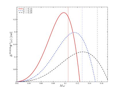
Figure 2: Difference between the 2.5PN-expanded tidal (Fourier) phase and the corresponding exact EOB one obtained by integrating Eq. (20). Each curve refers to a $\gamma=2$ polytropic model with different compactness. The vertical lines indicate the corresponding contact frequency.

III Measurability of tidal parameters: theoretical discussion

III.1 Fisher matrix formalism

Under usual simplifying assumptions (Gaussian noise, sufficiently high SNR) the variance $\sigma_{{\kappa_{2}^{T}}}^{2}$ in the measurement of ${\kappa_{2}^{T}}$ is computed using the standard Fisher matrix formalism, as already used in the context of binary systems in Refs. Cutler:1994ys ; Poisson:1995ef ; Flanagan:2007ix ; Hinderer:2009ca ; Pannarale:2011pk . When considering a Fourier–domain waveform $\tilde{h}(f;\,\lambda_{i})$ that is a function of $n+1$ parameters $\{\lambda_{i}\}=\{\lambda_{a},\lambda_{T}\}$, the Fisher information matrix is a $(n+1)\times(n+1)$ matrix whose elements are given by

$$F_{ij}\,=\,\langle\partial_{\lambda_{i}}h,\partial_{\lambda_{j}}h\rangle$$ (40)

where $\langle,\rangle$ denotes the Wiener scalar product between two signal $\tilde{h}(f)$ and $\tilde{k}(f)$, defined as

$$\langle h,k\rangle\equiv 4\,\Re\,\int\limits_{0}^{+\infty}df\dfrac{\tilde{h}^{*}(f)\tilde{k}(f)}{S_{n}(f)},$$ (41)

with $S_{n}(f)$ denoting the one-sided strain noise of the detector. In absence of specific prior, the variance in the measurement of each parameter $\lambda_{i}$ is given by the corresponding diagonal element of the inverse Fisher matrix (or covariance matrix),

$$\sigma_{\lambda_{i}}^{2}=(F^{-1})^{ii}.$$ (42)

Assuming the SPA approximation and neglecting relativistic corrections to the amplitude, the Fourier transform of the waveform is

$$\tilde{h}(f)=Af^{-7/6}e^{-{\rm i}\Psi(f)}\theta(f^{\rm contact}-f),$$ (43)

where $\theta(f^{\rm contact}-f)$ denotes a Heaviside step function indicating that we cut off the inspiral signal above the contact frequency defined above in Eq. (36).[ This is a coarse approximation to the post-merger signal that might be improved by extending the EOB representation to an effective description of the post-contact GW signal]. The amplitude parameter $A$ has been shown to be uncorrelated to the other parameters Cutler:1994ys ; Poisson:1995ef , so that we shall forget about it in the following.

From this equation, the squared signal to noise ratio (SNR) is written as

$$\rho^{2}=4\,\int\limits_{0}^{+\infty}df\dfrac{|\tilde{h}(f)|^{2}}{S_{n}(f)}=4\,A^{2}\int\limits_{0}^{{f^{\rm c}}}df\dfrac{f^{-7/3}}{S_{n}(f)},$$ (44)

where $f^{c}\equiv f^{\rm contact}$, and the elements of the Fisher matrix are

$$F_{ij}=4\,A^{2}\,\int\limits_{0}^{{f^{\rm c}}}\dfrac{df}{S_{n}(f)}f^{-7/3}\partial_{\lambda_{i}}\Psi\partial_{\lambda_{j}}\Psi$$ (45)

In view of the common proportionality of both $\rho^{2}$ and $F_{ij}$ to the (randomly vaying) squared signal amplitude $A^{2}$, it is convenient to define the following “reduced” Fisher matrix

$$\hat{F}_{ij}\equiv\dfrac{F_{ij}}{\rho^{2}}.$$ (46)

One then sees that this reduced Fisher matrix can be written as

$$\hat{F}_{ij}=\int\limits_{0}^{f^{\rm c}}df\,\gamma(f)\,\partial_{\lambda_{i}}\Psi(f)\partial_{\lambda_{j}}\Psi(f),$$ (47)

whre $\gamma(f)df$ denotes the following measure

$$\gamma(f)df\equiv\dfrac{df\,f^{-7/3}S_{n}^{-1}(f)}{\int\limits_{0}^{{f^{\rm c}}}df\,f^{-7/3}S_{n}^{-1}(f)}.$$ (48)

Note that this measure is normalized to unity, $\int\limits_{0}^{{f^{\rm c}}}\gamma(f)df=1$. This measure naturally leads to defining a new (Euclidean) scalar product among real phase functions

$$(a|b)\equiv\int\limits_{0}^{f^{\rm c}}df\gamma(f)\,a(f)\,b(f),$$ (49)

in terms of which we can write the rescaled Fisher matrix as

$$\hat{F}_{ij}=\left(\partial_{\lambda_{i}}\Psi|\partial_{\lambda_{j}}\Psi\right).$$ (50)

The elements of the inverse of this reduced Fisher matrix then give the “SNR-normalized probable errors”, $\rho\,\sigma_{\lambda_{i}}$ on each parameter, namely

$$\hat{\sigma}_{\lambda_{i}}\equiv\rho\,\sigma_{\lambda_{i}}=\sqrt{(\hat{F}^{-1})^{ii}}.$$ (51)

In the following $S_{n}$ is taken to be the ${\tt ZERO\_DET\_high\_P}$ anticipated sensitivity curve of Advanced Ligo shoemaker . The minimum of the effective dimensionless strain noise $fS_{n}(f)$ for this sensitivity curve is located at frequency $f_{0}=56.56$ Hz. In the following we shall often work with the reduced frequency parameter ${\hat{f}}\equiv f/f_{0}$.

III.2 Phasing model and parameter dependence

Concretely, we shall use a Fourier domain waveform of the type of Eq. (43), with a phase $\Psi(f)$ in the form

$$\Psi(f)=\Psi^{0}(f)+\Psi^{T}(f),$$ (52)

where, as above, $\Psi^{0}(f)$ denotes the point-mass contribution to the SPA phase and $\Psi^{T}(f)$ the tidal part. We shall approximate both contributions with some PN expansion. As already discussed above, the tidal contribution will be approximated by the 2.5PN accurate expression of Eq. (II.3). Concerning the point-mass phase, it is currently analytically known up to 3.5PN order Damour:2002kr ; Buonanno:2009zt . As we shall further discuss below, for the purpose of the present paper it will be enough to use the following 2PN Blanchet:1995ez accurate representation of the point-mass phase

$$\Psi^{0}\left({\hat{f}};\,\lambda_{1},\lambda_{2},\lambda_{3},\lambda_{4},\beta,\sigma\right) =\lambda_{1}+2\pi{\hat{f}}\lambda_{2}$$

$$+\frac{3}{128}(\pi\lambda_{3}f_{0}{\hat{f}})^{-5/3}\bigg{[}1+\frac{20}{9}\left(\frac{743}{336}+\frac{11}{4}\lambda_{4}\right)v_{\lambda_{3},\lambda_{4}}^{2}{\hat{f}}^{2/3}-4(4\pi-\beta)v_{\lambda_{3},\lambda_{4}}^{3}{\hat{f}}$$

$$+10\left(\dfrac{3058673}{1016064}+\dfrac{5429}{1008}\nu+\dfrac{617}{144}\nu^{2}-\sigma\right)v_{\lambda_{3},\lambda_{4}}^{4}{\hat{f}}^{4/3}\bigg{]},$$ (53)

where

$$v_{\lambda_{3},\lambda_{4}}\equiv\left(\pi\lambda_{3}\lambda_{4}^{-3/5}f_{0}\right)^{1/3}$$ (54)

and where the parameters the $(\lambda_{i})_{[1..4]}$ have the following meaning

$$\lambda_{1} =-\phi_{c}-\pi/4,$$ (55)

$$\lambda_{2} =f_{0}t_{c},$$ (56)

$$\lambda_{3} ={\cal M},$$ (57)

$$\lambda_{4} =\nu.$$ (58)

Here $\phi_{c}$ is a reference phase and $t_{c}$ a reference time, ${\cal M}\equiv\nu^{3/5}M$ is the chirp mass and $\nu=M_{A}M_{B}/M^{2}$ the symmetric mass ratio. In addition, the parameter $\beta$ is a spin-orbit parameter and $\sigma$ a spin-spin one.

As for the (quadrupolar) tidal contribution $\Psi^{T}(f)$ we can write it in various forms depending on the choice of tidal parameters we want to fit for. For instance, if we choose as tidal parameter $\lambda_{T}$ determining the overall scale of the tidal phase the following symmetric combination of the two $\ell=2$ tidal polarizability coefficients $G\mu_{2}^{A,B}=(2/3)k^{A,B}_{2}R_{A,B}^{5}$ (with the dimensions of $[\rm length]^{5}$),

$$\lambda_{T} =G\bar{\mu}_{2}\equiv\frac{G}{26}\left[\left(1+12\frac{X_{B}}{X_{A}}\right)\mu_{2}^{A}+\left(1+12\frac{X_{A}}{X_{B}}\right)\mu_{2}^{B}\right]\,,$$ (59)

we obtain a tidal signal of the form

$$\Psi^{T}_{\rm 2.5PN}({\hat{f}};\,\lambda_{T},\lambda_{a})=-\lambda_{T}\frac{117}{8M_{\lambda_{3},\lambda_{4}}^{5}\lambda_{4}}v_{\lambda_{3},\lambda_{4}}^{5}{\hat{f}}^{5/3}\hat{\Psi}^{T}_{\rm 2.5PN}({\hat{f}};\lambda_{a}),$$ (60)

where $M_{\lambda_{3},\lambda_{4}}\equiv\lambda_{3}\lambda_{4}^{-3/5}$ denotes the total mass expressed as a function of the chirp mass $\lambda_{3}$ and the symmetric mass ratio $\lambda_{4}$. In this form the $\lambda_{a}$-dependence of the factor $v_{\lambda_{3},\lambda_{4}}^{5}/(M_{\lambda_{3},\lambda_{4}}^{5}\lambda_{4})$ introduces correlations when fitting for $\lambda_{T}$ together with the $\lambda_{a}$’s. An alternative choice might be to consider as tidal parameter the (dimensionless) combination

$$\lambda_{T}^{\prime}=G\bar{\mu}_{2}\frac{v_{\lambda_{3},\lambda_{4}}^{5}}{M_{\lambda_{3},\lambda_{4}}^{5}\lambda_{4}},$$ (61)

so as to minimize the correlations when fitting $\lambda_{T}^{\prime}$ together with the $\lambda_{a}$’s. Note, however, that there will always remain correlations due to the $\lambda_{a}$-dependence in the fractional PN correction factor $\hat{\Psi}^{T}_{\rm 2.5PN}({\hat{f}};\lambda_{a})$. The $\lambda_{a}$-dependence of $\hat{\Psi}^{T}_{\rm 2.5PN}({\hat{f}};\lambda_{a})$ has several sources: i) an explicit dependence on ${\cal M}$ and $\nu$ coming through the argument $v=v_{\lambda_{3},\lambda_{4}}{\hat{f}}^{1/3}$; ii) an implicit dependence on the mass ratio coming from the individual Love numbers and the radii entering the definition of $\hat{\Psi}^{T}_{\rm 2.5PN}$ (see Appendix B). However, when computing the corresponding Fisher-matrix elements involving the partial derivative with respect to $\lambda_{a}$ of $\Psi$, the contributions from the $\lambda_{a}$-dependence of the tidal part $\Psi^{T}$ are largely subdominant compared to the large, early-inspiral dominating contribution coming from $\partial_{\lambda_{a}}\Psi^{0}$. We have indeed checked that taking into account the variability of the $\lambda_{a}$’s within $\hat{\Psi}_{\rm 2.5PN}^{T}({\hat{f}};\,\lambda_{a})$ or neglecting it only changes the error $\sigma_{\lambda_{T}}$ at the $1.5\times 10^{-3}$ fractional level. As for the $\lambda_{a}$ variability of the prefactor of $\hat{\Psi}^{T}_{\rm 2.5PN}$ in Eq. (60), when using (59) as tidal parameter, it was found (when $\beta$ and $\sigma$ are fixed, or well constrained), because of the signs of the correlations between $\lambda_{T}$ and $\lambda_{a}$, to lead to a small, ${\cal O}(2\%)$, improvement in the measurability of $\lambda_{T}$ compared to that of $\lambda^{\prime}_{T}$ given by Eq. (61). In the following we shall fit for $\lambda_{T}$, Eq. (59), taking into account the variability of the $\lambda_{a}$’s in the prefactor of the tidal phase [as displayed in Eq. (60)], however, for simplicity (and easier comparison with the unequal-mass case discussed below) we shall neglect the variability of the $\lambda_{a}$’s entering the PN-correction factor $\hat{\Psi}^{T}_{\rm 2.5PN}({\hat{f}};\,\lambda_{a})$, (i.e. neglect their small contribution to $\partial_{\lambda_{a}}\Psi^{T}$ computing the Fisher matrix).

In this work we keep in the tidal signal $\Psi^{T}_{\rm 2.5PN}(f)$ only the contribution associated to the quadrupolar tidal deformation as measured by $\kappa_{2}^{A}$ or $G\mu_{2}^{A}$. Actually, the EOB formalism takes into account higher multipolar tidal interactions, as already done in previous work Damour:2009wj ; Baiotti:2010xh ; Baiotti:2011am . Using this theoretical result, we show however in Appendix A.2 that the numerical contribution of higher multipole moments ($\ell=3,4$) to the tidal signal is rather small ($\Delta\Psi^{T}\sim-0.2$ rad), so that we are entitled to neglect it to estimate the measurability of ${\kappa_{2}^{T}}$. However, we recommend that in fitting real GW signals to tidal EOB templates one includes also the higher multipolar tidal contributions. But, in order not to introduce new parameters to be fitted, one should express the higher-order polarizability parameters, $G\mu_{\ell}$, in terms of $G\mu_{2}$ only. More precisely, using $G\mu_{2}\sim k_{2}R^{5}$, $G\mu_{3}\sim k_{3}R^{7}$ and $G\mu_{4}\sim k_{4}R^{9}$, one can reexpress $G\mu_{3}$ and $G\mu_{4}$ in terms of $G\mu_{2}$ and of the following combination of Love numbers

$$k_{3/2}\equiv\dfrac{k_{3}}{k_{2}^{7/5}}$$ (62)

$$k_{4/2}\equiv\dfrac{k_{4}}{k_{2}^{9/5}}$$ (63)

e.g., $G\mu_{3}\sim k_{3/2}\,(G\mu_{2})^{7/5}$. Replacing then the modified Love numbers $k_{3/2}$ and $k_{4/2}$ by some constant numbers (say of order 0.7 so as to approximately mimick the result of realistic EOSs) we end up with an approximate description of higher multipolar contributions that is entirely expressed in terms of the quadrupole polarizability parameter $G\mu_{2}$.

Let us now comment on the form, Eq. (III.2), of the point-mass phase that we shall use in this work. This point-mass phase is only 2PN accurate. The reason for limiting our accuracy to this level is that, as we will see explicitly below, the terms in the Fisher matrix that determine the measurability of the two dynamical parameters entering the point-mass phase, namely the chirp mass $\lambda_{3}={\cal M}$ and the symmetric mass ratio $\lambda_{4}=\nu$, are essentially proportional to integrals of the following types: $I_{-10}=\int d\ln f\,f\gamma(f)v(f)^{-10}$ and $I_{-6}=\int d\ln f\,f\gamma(f)v(f)^{-6}$. While the integral giving the signal to noise ratio, Eq. (44) is proportional to $I_{0}=\int d\ln ff\gamma(f)$ and is roughly concentrated around a couple of frequency octaves around ${\hat{f}}=f/f_{0}=1$, the integrals $I_{-10}$ and $I_{-6}$ are mainly concentrated towards (different) lower frequencies.

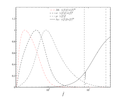
Figure 3: Integrands, per frequency octave, of the integrals determining the measurability of ${{\cal M}}$, $\nu$, $\rho$ (SNR) and $\lambda_{T}$. While most of the SNR is gathered around frequencies ${\hat{f}}=f/(56.56~{}{\rm Hz})\sim 1$, the measurability of ${\cal M}$ and $\nu$ is concentrated towards lower frequencies (${\hat{f}}=f/f_{0}<1$), and that of the tidal parameter $\lambda_{T}$ gets its largest contribution from the late inspiral up to the merger. The rightmost vertical line indicates the merger frequency for ${\cal C}=0.1645$, while the leftmost vertical line marks 450 Hz for a $1.4M_{\odot}+1.4M_{\odot}$ BNS system.

The concentration on the logarithmic frequency axis of several relevant measurability signals is illustrated in Fig. 3. Note in particular how the integrands of $I_{-10}$ (chirp mass) and $I_{-6}$ (symmetric mass ratio) are peaked at frequencies below the SNR integrand of $I_{0}$. Physically, this corresponds to saying that most of the useful cycles for the measurability of ${\cal M}$ and $\nu$ come from the early inspiral. As the PN expansion converges reasonably well for such low frequencies, using a 2PN accurate phasing is guaranteed to be a reasonably good approximation for the point-mass part of the phase. This has been checked by Ref. Poisson:1995ef for the measurement of ${\cal M}$ and $\nu$, which found (see their Table II) that using a 2PN accurate (instead of a 1.5PN accurate, as in Ref. Cutler:1994ys ) template led to only $\sim 10\%$ differences in the fractional uncertainties in $\nu$ and ${\cal M}$. We found, as expected, that the situation is even better for the measurement of $\lambda_{T}$: namely, we found that the fractional uncertainty on $\lambda_{T}$ is changed (and actually improved) when using a 2PN template for $\Psi^{0}$, rather than a 1.5PN one, only at the $5\times 10^{-3}$ level By contrast to the cases of ${\cal M}$ and $\nu$, the measurability of the tidal parameter $\lambda_{T}$ is associated in the Fisher matrix to an integral of the type $I_{+10}=\int d\ln ff\gamma(f)v(f)^{10}$, which gets its largest contribution from the late inspiral up to the merger (see solid line in Fig. 3). More specifically, the integrand of $I_{+10}$, i.e. $\propto f\gamma(f)f^{10/3}$ is equal to $f^{2}/S_{n}(f)$. The ${\tt ZERO\_DET\_high\_P}$ advanced LIGO noise curve $S_{n}(f)$ happens to be a rather flat function of $f$ between $\sim 50$ Hz and $\sim 800$ Hz and then increases to reach a shot noise behavior $S_{n}(f)\propto f^{2}$ at high frequencies. This implies that the integrand of $I_{+10}$, i.e. $f^{2}/S_{n}(f)$, roughly grows like $f^{2}$ between 50 Hz and 800 Hz, to then asymptote towards a finite limit at high frequencies. The clear separation between, on the one hand, the two SNR curves associated to ${\cal M}$ and $\nu$ (which are relatively close to each other) and on the other hand the SNR curve associated to $\lambda_{T}$ also indicates (as we shall discuss below) that ${\cal M}$ and $\nu$ are strongly correlated among themselves, while $\lambda_{T}$ is not so strongly correlated to ${\cal M}$ and $\nu$. The figure also displays two possible cut-off frequencies for the measurements of the tidal signal: the conservative value 450 Hz (dashed vertical line) used in Refs. Flanagan:2007ix ; Hinderer:2009ca , ${\hat{f}}=7.956$, or the compactness–dependent contact frequency that we shall use here, $(\pi Mf)_{\rm contact}={\cal C}^{3/2}$ (dash-dotted vertical line, computed using EOS BSK21 with a model with $M=1.4M_{\odot}$ and ${\cal C}=0.1645$). Evidently, the use of the late-inspiral cut-off frequency ${\hat{f}}_{\rm contact}$ calls for a formalism able to describe the phasing up to the merger (here, the EOB formalism and its accurate high PN expanded representation discussed in the previous section).

In Eq. (III.2) we have included also a parameter $\beta$ associated to the spin-orbit interaction and a parameter $\sigma$ associated to the spin-spin one Blanchet:1995ez . These parameters are equal to

$$\beta =\dfrac{1}{12}\left(113X_{A}^{2}+75\nu\right){\bf\hat{L}}\cdot{\bf\hat{a}}_{A}+(A\leftrightarrow B),$$ (64)

$$\sigma =\dfrac{\nu}{48}\left(-247{\bf\hat{a}}_{A}\cdot{\bf\hat{a}}_{B}+721\,{\bf\hat{L}}\cdot{\bf\hat{a}}_{A}\,{\bf\hat{L}}\cdot{\bf\hat{a}}_{B}\right),$$ (65)

where ${\bf\hat{a}}_{A}={\bf S}_{A}/(GM_{A}^{2})$ is the dimensionless spin parameter of body $A$. Previous work Cutler:1994ys ; Poisson:1995ef ; Hinderer:2009ca discussing data-analysis including the spin parameters $\beta$ and $\sigma$ had incorporated Bayesian priors à la Cutler:1994ys constraining the magnitudes of $|\beta|$ and $|\sigma|$ to be smaller than $8.5$ and $5.0$ respectively, which are plausible theoretical upper limits on them. However, such values are very conservative bounds on $\beta$ and $\sigma$ in view of observed binary pulsar systems (as already pointed out in Refs. Cutler:1994ys ; Blanchet:1995ez ). Indeed, recent estimates of the event-rate for BNS GW observations are mainly obtained from extrapolation of the currently observed binary pulsar systems. All the known binary pulsar systems have rather small observed spin parameters. Considering the fastest spinning pulsar observed in a BNS system, namely PSR J0737-3039A, whose spin period is 23 ms Lorimer:2008se , we concluded from the calculations of moments of inertia by Bejger et al. Bejger:2005jy (who work with the EOSs: BPAL12, APR, SLy, BGN2H1 and GNH3) and by Morrison et al.Morrison:2004df (who use FPS), that the initial dimensionless spin parameter $\hat{a}$ is between approximatively $0.017$ (for BPAL12) and $0.03$ (for GNH3). This leads to an initial range for the corresponding parameter $\beta$ of order $|\beta|\,\in\,\left[0.11;0.196\right]$, while the 2PN-level spin-spin parameter $\sigma$ is at most of the order $|\sigma|\lesssim 10^{-4}$. Taking into account the slowing down of the spin until the moment of merger, we estimated that $\beta$ at the time of the merger would be within the range $[0.09;0.17]$ so that we decided to use the conservative upper limit of $0.2$ for $\beta$. Hence, we studied the measurability of $\beta$ together with the five other parameters $\{\lambda_{1,\dots,4};\,\lambda_{T}\}$ submitted to a Gaussian Bayesian prior $\propto\exp[-1/2(\beta/0.1)^{2}]$ constraining $|\beta|$ to be smaller than 0.2 at the $95\%$ confidence level. The result of the error estimates coming from such a constrained, six-parameter Fisher matrix formalism will be presented in Table 2 below, where they are compared to the result of a five-parameter Fisher matrix formalism where $\beta$ is set to zero from the beginning. One sees from the numbers in Table 2 that such a constrained six-parameter analysis leads to only a very slight increase of the error estimates. In view of this, in the following we shall neglect (i.e. set to zero from the start) $\beta$. Similarly, and a fortiori, in view of the very small upper bound quoted above on $\sigma$, we can also neglect the 2PN level spin-spin parameter $\sigma$. Let us emphasize that if, by contrast, one keeps the parameter $\beta$ while using the very conservative prior $\beta\leq 8.5$, this leads to a very large increase of the error bars on ${\cal M}$ and $\nu$, and a noticeable increase of the error bar on $\lambda_{T}$. As it will be exemplified in Table 2, the use of the very conservative prior constraining $\beta\leq 8.5$ instead of the “realistic” one leading to $\beta\leq 0.2$, increases the statistical measurement error on $G\mu_{2}$ by a factor which varies between 1.28 (for EOS BSK19) and 1.10 (for EOS GNH3). In addition, if one does not neglect the spin-spin parameter $\sigma$ (as we shall do here), or alternatively, does not put a realistic prior on it, but instead fits for it using a seven parameter Fisher matrix, constrained by the very conservative bound $|\sigma|<5.0$, this leads to a further, substantial increase of the measurement errors.

IV Measurability of tidal parameters: numerical results

IV.1 A sample of equations of state

Table 1: Properties of a $M_{A}=1.4M_{\odot}$ neutron star for the 11 EOSs considered in this paper. From left to right, the columns report: the name of the EOS; the radius of the star $R$; its compactness ${\cal C}$; the value of the $\ell=2$ Love number $k_{2}$; the value of the tidal parameters ${\kappa_{2}^{T}}$ and $G\mu_{2}$; the value of the bare contact frequency $f^{\rm c}_{\rm bare}$ in Hz and the corresponding dimensionless contact frequency ${\hat{f}}^{\rm c}_{\rm bare}=f^{\rm c}_{\rm bare}/f_{0}$ with $f_{0}=56.56$ Hz.

EOS	$R$ [km]	${\cal C}$	$k_{2}$	$\kappa_{2}^{T}$	$G\mu_{2}~{}[{\rm km}^{5}]$	$f^{\rm c}$ [Hz]	${\hat{f}}^{\rm c}$
MS1	14.92	0.1390	0.1100	264.9895	53360.36	1196.09	21.15
GNH3	14.19	0.1457	0.0852	162.099	32641.6	1284.06	22.702
MS2	13.71	0.1510	0.0883	140.6002	28312.35	1354.28	23.94
BSK21	12.57	0.1645	0.0930	96.4647	19424.9	1540.29	27.23
MPA1	12.47	0.1660	0.0924	91.6308	18451.49	1561.00	27.60
AP3	12.09	0.1710	0.0858	73.3528	14770.89	1632.06	28.85
BSK20	11.75	0.1760	0.0810	59.8628	12054.4	1704.83	30.14
SLy	11.74	0.1766	0.0767	55.8421	11244.8	1712.55	30.2785
APR	11.37	0.1819	0.0768	48.2159	9709.13	1790.2	31.6514
FPS	10.85	0.1907	0.0662	32.7966	6604.17	1922.7	33.99
BSK19	10.75	0.1924	0.0647	30.6662	6175.14	1948.14	34.444

In this paper we consider a sample of EOSs taken from the literature. The sample is chosen to include EOS with a large range of variation in radius $R$, Love number $k_{2}$ and tidal parameter $G\mu_{2}$. We consider eleven state-of-the-art EOSs. Seven among them, namely, MS1, MS2 Mueller:1996pm , MPA1, AP3 PhysRevC.58.1804 , APR, SLy and FPS, have normal matter content ($npe\mu$). One, namely GNH3 Glendenning:1984jr , also incorporates some mixture of hyperons, pion condensates and quarks. Finally, the three labels BSK19, BSK20 and BSK21 refer to Skyrme–force–related energy density functionals (fitted to nuclear mass data) from which one can compute the EOS of cold neutron star matter Chamel:2011aa . Among these equations of state, seven of them (MS1, MS2, MPA1, AP3, SLy, FPS and GNH3) have been used in Ref. Hinderer:2009ca . Table 1 lists, by order of decreasing radius (or increasing compactness) the main characteristics of Tolman-Oppenheimer-Volkoff neutron star models built from these EOS having mass $1.4M_{\odot}$. These NS properties were computed starting from the tabulated EOS, using Hermite polynomials interpolation Bernuzzi:2008fu , for all EOS but (MS1, MS2, MPA1, AP3), that we read instead from Table I of Ref. Hinderer:2009ca . In our Table 1, ${\kappa_{2}^{T}}$ refers to a fiducial $1.4M_{\odot}+1.4M_{\odot}$ binary system and $f^{\rm c}\equiv f^{\rm contact}$ refers to the contact frequency defined above (see Eq. (36)). Note that ${\kappa_{2}^{T}}$ and $G\mu_{2}$ decrease correlatively with the radius due to the dominant influence of the fifth power of the radius in ${\kappa_{2}^{T}}$ and $G\mu_{2}$, and in spite of the nonmonotonic behavior of $k_{2}$. The fifth root of $G\mu_{2}$ defines a length scale which we can call the tidal radius of the NS. It is related to the radius $R$ according to

$$R_{\rm tidal}\equiv\left(G\mu_{2}\right)^{1/5}=\left(\dfrac{2}{3}k_{2}\right)^{1/5}R.$$ (66)

The values of the tidal radius for the $1.4M_{\odot}$ models listed in Table 1 vary between 8.8195 km (for MS1) and 5.7297 km (for BSK19). The median value is around 7 km. In the following we shall focus on a subsample of the EOS listed above, namely we shall consider only GNH3, BSK21, BSK20, SLy, APR, FPS and BSK19, which span a plausible subrange of values of $G\mu_{2}$ (note that we conservatively eliminate for instance the very stiff EOS MS1 which yields an extremely large value of $G\mu_{2}$).

IV.2 Measurability of $G\mu_{2}$: equal-mass case

In this section we focus on the measurability of tidal parameters in equal-mass BNS systems. We shall see below that, within the reasonable range of mass ratios expected from observational data, this equal-mass study is a sufficiently accurate indicator of the general case.

Among the EOSs listed in the previous section, two of them (FPS and BSK19), which would have given the two smallest values of $G\mu_{2}$, lead to maximum neutron star masses which are smaller than the recently reported value Demorest:2010bx $M_{\rm NS}=(1.97\pm 0.04)M_{\odot}$. Because of this we shall first discuss the measurability of tidal parameters within the restricted, observationally compatible, EOS subsample GNH3, BSK21, BSK20, SLy, APR. For each of these EOS we computed the $5\times 5$ reduced Fisher matrix $\hat{F}_{ij}$, Eq. (47), corresponding to the parameters $[\lambda_{1},\dots,\lambda_{4};\,\lambda_{T}]$ where the first four parameters refer to the binary system (see Eqs. (55)-(58)), while the tidal parameter $\lambda_{T}$, defined in Eq. (59), reduces simply to $G\mu_{2}=G\mu_{2}^{A}=G\mu_{2}^{B}$ in the equal-mass case. The computation of the Fisher matrix elements is performed by considering that the GW signal is cut off above the (compactness dependent) contact frequency, Eq. (36), i.e. each integral is taken over the frequency window $[f_{\rm min},f_{\rm max}]$, with $f_{\rm min}=10$ Hz and $f_{\rm max}=f_{\rm contact}$.

The diagonal elements of the inverse of the matrix $\hat{F}_{ij}$ yield, according to Eq. (51), the SNR-normalized probable (statistical) errors $\hat{\sigma}_{\lambda_{i}}\equiv\rho\sigma_{\lambda_{i}}$ on each parameter $\lambda_{i}$. Before discussing the measurability of the nontidal parameters, let us start by considering the measurability of the tidal parameter $\lambda_{T}=G\mu_{2}$.

Figure 4: Measurability of the tidal polarizability parameter $G\mu_{2}$ (in units of km⁵) as a function of the neutron star mass for a sample of realistic EOS from Table 1. This plot refers to the observation (at the SNR level $\rho=16$) of the gravitational wave signal from an equal-mass BNS merger as seen by a single advanced LIGO detector. The solid lines represent the values of $G\mu_{2}$ as a function of the NS mass, while the dashed lines represent the $1~{}\sigma$ ($68\%$ confidence level) expected statistical errors. The vertical line marks the canonical NS mass $1.4M_{\odot}$. Note that over a wide range of masses each solid line lies comfortably above the corresponding measurability threshold, therefore indicating that the advanced LIGO-Virgo detector network can significantly measure $G\mu_{2}$.

Table 2: Measurability of the tidal parameter $G\mu_{2}$ for a $M=1.4M_{\odot}+1.4M_{\odot}$ neutron star binary obtained using the TaylorF2 frequency-domain approximant to the phase, truncated at 2.5PN fractional accuracy for the tidal part and at 2PN accuracy in the point-mass part. From left to right the columns report: the name of the EOS; the value of the spin-orbit parameter and of the prior on it; the radius of the star; its compactness; the value of the $\ell=2$ tidal parameter $G\mu_{2}$; the SNR-normalized relative errors on the chirp mass $\hat{\sigma}_{\cal M}/{\cal M}$ and on the $\nu$ parameter $\hat{\sigma}_{\nu}/\nu$ when cutting at bare contact frequency; the SNR-normalized absolute error, $\hat{\sigma}_{G\mu_{2}}$, and relative error $\hat{\sigma}_{G\mu_{2}}/(G\mu_{2})$ on $G\mu_{2}$. The last two columns refer to the absolute and relative errors on $G\mu_{2}$ that are obtained by taking as cut-off frequency the conservative value 450Hz.

EOS	$\beta$	$R$ [km]	${\cal C}$	$G\mu_{2}\,[{\rm km}^{5}]$	$\hat{\sigma}_{\ln{\cal M}}$	$\hat{\sigma}_{\ln\nu}$	$\hat{\sigma}_{G\mu_{2}}$ [km5]	$\hat{\sigma}_{\ln G\mu_{2}}$	$\hat{\sigma}_{G\mu_{2}}^{450\rm Hz}$ [km5]	$\hat{\sigma}_{\ln G\mu_{2}}^{450\rm Hz}$
GNH3	$|\beta|<+\infty$	14.19	0.1457	32641.6	0.00415853	3.18959	186 292	5.70720	1 476 380	45.23
	$|\beta|<8.5$	14.19	0.1457	32641.6	0.00405962	3.09906	182 612	5.59447	1 236 580	37.8835
	$|\beta|<0.2$	14.19	0.1457	32641.6	0.000447397	0.122751	165 714	5.07679	874 001	26.7757
	$\beta=0$	14.19	0.1457	32641.6	0.000450135	0.117804	165 652	5.07487	873 019	26.7456
BSK21	$|\beta|<+\infty$	12.57	0.1645	19424.9	0.003946	2.98317	158 080	8.13801	1 539 610	79.2596
	$|\beta|<8.5$	12.57	0.1645	19424.9	0.0038749	2.91796	155 190	7.98922	1 284 240	66.1132
	$|\beta|<0.2$	12.57	0.1645	19424.9	0.000434397	0.115657	133 108	6.85246	876 337	45.1141
	$\beta=0$	12.57	0.1645	19424.9	0.000436901	0.110806	133 046	6.84928	875 290	45.0603
BSK20	$|\beta|<+\infty$	11.75	0.1760	12054.4	0.00384331	2.88426	148 380	12.3092	1 575 360	130.687
	$|\beta|<8.5$	11.75	0.1760	12054.4	0.00378349	2.82927	145 750	12.0910	1 311 380	108.788
	$|\beta|<0.2$	11.75	0.1760	12054.4	0.000428026	0.112247	118 815	9.85656	877 640	72.8064
	$\beta=0$	11.75	0.1760	12054.4	0.000430414	0.107437	118 751	9.85125	876 558	72.7166
SLy	$|\beta|<+\infty$	11.74	0.1766	11244.8	0.00383898	2.8801	148 911	13.2426	1 579 310	140.448
	$|\beta|<8.5$	11.74	0.1760	11244.8	0.00377961	2.82552	146 254	13.0064	1 314 390	116.888
	$|\beta|<0.2$	11.74	0.1760	11244.8	0.000427755	0.112104	118 271	10.5179	877 784	78.0612
	$\beta=0$	11.74	0.1760	11244.8	0.000430139	0.107295	118 206	10.5121	876 697	77.9646
APR	$|\beta|<+\infty$	11.37	0.1819	9709.13	0.00379747	2.84028	142 857	14.7136	1 586 810	163.434
	$|\beta|<8.5$	11.37	0.1819	9709.13	0.00374226	2.78947	140 408	14.4615	1 320 100	135.964
	$|\beta|<0.2$	11.37	0.1819	9709.13	0.000425161	0.110728	112 643	11.6018	878 055	90.436
	$\beta=0$	11.37	0.1819	9709.13	0.000427498	0.105935	112 580	11.5953	876 961	90.3233
FPS	$|\beta|<+\infty$	10.85	0.1907	6604.17	0.00373437	2.77992	135 473	20.5133	1 602 010	242.575
	$|\beta|<8.5$	10.85	0.1907	6604.17	0.00368509	2.73448	133 267	20.1792	1 331 690	201.644
	$|\beta|<0.2$	10.85	0.1907	6604.17	0.000421197	0.108641	104 424	15.8118	878 605	133.038
	$\beta=0$	10.85	0.1907	6604.17	0.000423462	0.103871	104 362	15.8025	877 496	132.87
BSK19	$|\beta|<+\infty$	10.75	0.1924	6175.14	0.00372323	2.76928	134 005	21.7007	1 604 110	259.769
	$|\beta|<8.5$	10.75	0.1924	6175.14	0.00367495	2.72475	131 846	21.3511	1 333 300	215.914
	$|\beta|<0.2$	10.75	0.1924	6175.14	0.000420494	0.108273	102 998	16.6795	878 681	142.293
	$\beta=0$	10.75	0.1924	6175.14	0.000422746	0.103507	102 937	16.6696	877 570	142.113

A recent summary Abadie:2010cf of the expected event rate of BNS coalescences suggests that at the standard SNR detection threshold $\rho=8$ a “realistic” estimate of the number of events per year detectable by the advanced LIGO-Virgo network is $\sim 40$. This means that at the SNR $\rho=16$ one can reasonably expect to detect $\sim 40/(2^{3})=5$ events per year. Considering such a SNR $\rho=16$ we plot in Fig. 4, for each of the five EOS selected above, the following two curves: (i) the value of the tidal parameter $G\mu_{2}$ (in $[{\rm km}^{5}]$) as a function of the mass of each NS (thick, solid lines); and (ii) the corresponding value of the absolute statistical error $\sigma_{G\mu_{2}}$ (in $[{\rm km}^{5}]$). To guide the eye, a vertical line indicates the “canonical” mass value $M=1.4M_{\odot}$. If we first focus on this mass value, this figure shows that a single advanced LIGO or Virgo detector can measure $G\mu_{2}$ for all considered EOS (with $M_{\max}\geq 1.97M_{\odot}$) at a signal to noise ratio $G\mu_{2}/\sigma_{G\mu_{2}}$ that varies between 1.4 for the APR EOS up to 3.1 for the GNH3 one .

For mass values smaller than $1.4M_{\odot}$ the measurability of $G\mu_{2}$ is even better (larger ratio between $G\mu_{2}$ and $\sigma_{G\mu_{2}}$), while for mass values larger than 1.4$M_{\odot}$ the measurability degrades. The intersection points in Fig. 4 between solid and dashed curves corresponding to the same EOS mark the value the mass where $G\mu_{2}$ is only measurable at the “$1\sigma$” ($68\%$ confidence) level, i.e., $\sigma_{G\mu_{2}}=G\mu_{2}$. For instance, for the APR EOS, still assuming a SNR $\rho=16$, equal-mass BNS systems with individual NS masses larger than $1.52M_{\odot}$ cannot allow one to extract $G\mu_{2}$ at a significant level. By contrast, in the case of BSK21 and GNH3 EOS one can extract tidal parameters for BNS systems up to individual masses larger than about $1.74M_{\odot}$.

In summary, Fig. 4 shows that gravitational wave observations from a single advanced detector are able to extract tidal parameters at a significant level, even for the soft EOSs that lead to the smallest values of $G\mu_{2}$. This conclusion strikingly contrasts with that of Hinderer et al. Hinderer:2009ca . We will discuss below the reasons behind this difference in conclusion.

To complement the graphical representation of our results in Fig. 4, we present in Table 2 numerical data referring not only to the $5\times 5$, spinless, Fisher matrix calculation behind this figure, but to other calculations. More precisely, this table gives SNR-normalized errors $\hat{\sigma}_{\lambda_{i}}$ for all parameters of direct physical significance, namely $\lambda_{3}={\cal M}$, $\lambda_{4}=\nu$ and $\lambda_{T}=G\mu_{2}$. [ Note that the numerical value of each $\hat{\sigma}_{\lambda_{i}}$ formally gives the error corresponding to a unit SNR, $\rho=1$. For larger values of $\rho$ the error has to be divided by $\rho$.]. This table now considers the larger sample of EOS made by GNH3, BSK21, BSK20, SLy, APR, FPS and BSK19. For each one of these EOS we computed a $6\times 6$ (or $5\times 5$, see below) reduced Fisher matrix $\hat{F}_{ij}$, Eq. (47), corresponding now to the parameters $[\lambda_{1},\dots,\lambda_{4};\,\beta;\,\lambda_{T}]$. Here, in addition to the first four binary–system parameters considered above and of the tidal parameter $\lambda_{T}$ we also consider the spin-orbit parameter $\beta$ (which will be treated with various different constraints, see below). We use the same frequency window ( $[f_{\rm min},f_{\rm max}]$, with $f_{\rm min}=10$ Hz and $f_{\rm max}=f_{\rm contact}$) as above. We now consider the diagonal elements of the inverse of the matrix $\hat{F}_{ij}$ for all the parameters of direct physical significance, namely $\lambda_{3}={\cal M}$, $\lambda_{4}=\nu$ and $\lambda_{T}=G\mu_{2}$, we list in Table 2 the corresponding SNR-normalized errors $\hat{\sigma}_{\lambda_{i}}$.

For each EOS, the results are displayed along four rows. On each row, the first four columns give: (i) information about the treatment of the spin-orbit parameter $\beta$; (ii) the value of the neutron star radius (in km); (iii) the value of the compactness; (iv) the value of the tidal parameter $G\mu_{2}$. The following four columns give: (v) the fractional, SNR normalized, error on the chirp mass $\hat{\sigma}_{\ln{\cal M}}\equiv\hat{\sigma}_{\cal M}/{\cal M}$; (vi) the fractional SNR normalized, error on the symmetric mass ratio, $\hat{\sigma}_{\ln\nu}\equiv\hat{\sigma}_{\nu}/\nu$; (vii) the absolute, SNR normalized error $\hat{\sigma}_{G\mu_{2}}$ on $G\mu_{2}$ (in $[{\rm km}^{5}]$); and finally (viii) the fractional, SNR normalized error $\hat{\sigma}_{\ln G\mu_{2}}\equiv\hat{\sigma}_{G\mu_{2}}/(G\mu_{2})$ on $G\mu_{2}$. Concerning the treatment of the spin-orbit parameter, the first row, labelled with $|\beta|<+\infty$ refers to a $6\times 6$ Fisher matrix analysis where $\beta$ is included as a sixth unconstrained parameter. The second row, $|\beta|<8.5$, refers to a a $6\times 6$ Fisher matrix analysis where $\beta$ is constrained by adding a Gaussian prior proportional to $\exp[-1/2(2\beta/8.5)^{2}]$. Similarly, the third row corresponds to a more constraining prior proportional to $\exp[-1/2(2\beta/0.2)^{2}]$. Finally, the fourth row corresponds to a $5\times 5$ Fisher matrix analysis where $\beta$ is set to zero from the beginning without being fitted for, which was used to obtain the data displayed in Fig. 4. As already mentioned above, the results for the strong prior $|\beta|<0.2$ (3rd row) are nearly indistinguishable from the results of the $5\times 5$ Fisher matrix analysis (4th row). This justifies our use of the $5\times 5$ Fisher matrix results in Fig. 4 above. By contrast, we see that the results corresponding either to the conservative prior $|\beta|<8.5$ (second row) or the lack of any prior (first row) are close to each other but differ from the strongly $\beta$-constrained results by very significant factors. To be precise, the measurability of the chirp mass is worsened by a factor larger than seven; that of the symmetric mass ratio is worsened by a factor of order 30!; finally, that of $G\mu_{2}$ is only worsened by about $20\%$. These results are linked to the different origins of the effective signals contributing to the measurability of the various parameters displayed in Fig. 3.

Table 3: Measurability of the tidal parameter $\bar{\mu}_{2}$, Eq. (59), for a $M=1.1529M_{\odot}+1.6470M_{\odot}$ neutron star binary ($M_{A}/M_{B}=0.7$) obtained using the TaylorF2 frequency-domain approximant at 2.5PN fractional accuracy in the tidal part of the phase and at 2PN accuracy in the point-mass part of the phase. From left to right the columns report: the name of the EOS; the compactnesses of the stars; the values of the $\ell=2$ tidal polarizability parameters $G\mu_{A}$ and $G\mu_{B}$ of the stars; the value of the tidal parameter $G\bar{\mu}_{2}$; the bare contact frequency $f^{\rm c}_{\rm bare}$ in Hz; the SNR-normalized relative errors on the chirp mass $\hat{\sigma}_{\cal M}/{\cal M}$ and on the $\nu$ parameter $\hat{\sigma}_{\nu}/\nu$; the absolute (in km⁵) and relative errors on $G\bar{\mu}_{2}$. For each EOS, the second row recalls the corresponding results for equal masses.

EOS	${\cal C}_{A}$	${\cal C}_{B}$	$G\mu_{2}^{A}[{\rm km}^{5}]$	$G\mu_{2}^{B}[{\rm km}^{5}]$	$G\bar{\mu}_{2}[{\rm km}^{5}]$	$f^{\rm c}_{\rm bare}$ [Hz]	$\hat{\sigma}_{\ln{\cal M}}$	$\hat{\sigma}_{\ln\nu}$	$\hat{\sigma}_{G\bar{\mu}_{2}}$ [km5]	$\hat{\sigma}_{\ln G\bar{\mu}_{2}}$
GNH3	0.118	0.178	41115.1	20711.1	36178.1	1301.97	0.000429438	0.115405	158 647	4.38517
GNH3	0.1457	0.1457	32641.6	32641.6	32641.6	1284.06	0.000450135	0.117804	165 652	5.07487
BSK21	0.1361	0.1938	22049.1	15623.7	21034.5	1547.11	0.000417681	0.108921	129 240	6.1442
BSK21	0.1645	0.1645	19424.9	19424.9	19424.9	1540.29	0.000436901	0.110806	133 046	6.84928
BSK20	0.1446	0.2091	14638.3	8891.9	13429.4	1713.76	0.00041153	0.105588	115 330	8.5879
BSK20	0.1760	0.1760	12054.4	12054.4	12054.4	1704.83	0.000430414	0.107437	118 751	9.85125
SLy	0.144	0.2116	14347.3	7696.2	12794.1	1723.62	0.000411201	0.105412	114 634.	8.95991
SLy	0.1760	0.1760	11244.8	11244.8	11244.8	1712.55	0.000430139	0.107295	118 206	10.5121
APR	0.14934	0.2157	11874.0	7144.9	10868.9	1797.14	0.000408861	0.104155	109 549	10.0792
APR	0.1819	0.1819	9709.13	9709.13	9709.13	1790.2	0.000427498	0.105935	112 580	11.5953
FPS	0.154	0.2345	9443.33	3433.1	7830.8	1956.63	0.000404363	0.101758	100 125	12.7862
FPS	0.1907	0.1907	6604.17	6604.17	6604.17	1922.7	0.000423462	0.103871	104 362	15.8025
BSK19	0.1553	0.2352	8866.4	3386.96	7411.5	1973.3	0.000403933	0.101529	99 261	13.3929
BSK19	0.1924	0.1924	6175.14	6175.14	6175.14	1948.14	0.000422746	0.103507	102 937	16.6696

We can roughly summarize the results for the measurability of the nontidal parameters (in the strongly constrained $\beta$ cases) in the following way:

$$\dfrac{\sigma_{\cal M}}{{\cal M}}\approx\dfrac{4.3\times 10^{-4}}{\rho},$$ (67)

and

$$\dfrac{\sigma_{\nu}}{\nu}\approx\dfrac{0.11}{\rho}.$$ (68)

For instance, when $\rho=10$ this means that the chirp mass is measured to a fractional precision of $4\times 10^{-5}$, while the symmetric mass ratio is measured at a fractional precision of 0.01. As usual, the fractional precision on ${\cal M}$ is excellent (and has not been very significantly worsened by the inclusion of the tidal term, as shown by comparing to the results of Refs. Cutler:1994ys ; Poisson:1995ef ). By contrast, the fractional precision on $\nu$ has been significantly worsened (by a factor of order $1.7$) compared to Refs. Cutler:1994ys ; Poisson:1995ef when fitting for an extra tidal parameter. This worsening in the measurability of $\nu$ might make it difficult to distinguish stars with a mass ratio between 0.75 and 1. For instance, if we considered a BNS with $M_{A}=1.2M_{\odot}$, $M_{B}=1.6M_{\odot}$ (i.e., $M_{A}/M_{B}=0.75$) its symmetric mass ratio is $\nu\approx 0.2449$, so that $1-4\nu=0.0204$, corresponding to a fractional $\delta\nu/\nu\approx 0.02$. Comparing this with the measurement error in $\nu$ for $\rho=8$, Eq. (68), this is only a $2\sigma$-level deviation. Actually, this problem may be cured by doing two separate analyses of the GW data, one using inspiral data only up to a cut-off frequency small enough to be able to neglect tidal effects (without trying to fit for tidal parameters), which will probably give a better estimate of the mass ratio. And a separate analysis of the data up to (and possibly beyond) the merger aimed at extracting EOS–dependent information.

The last two columns of the table exhibit the SNR-normalized absolute and relative errors on $G\mu_{2}$ in the case where one uses as upper frequency cut-off $f_{\rm max}=450$ Hz as done in Ref. Hinderer:2009ca ; Flanagan:2007ix . The use of such a lower cut-off leads to a dramatic worsening (by a factor $\sim 7$) of the measurability of $G\mu_{2}$ (the origin of this worsening is illustrated in Fig. 2, which includes a line at 450 Hz).

On the other hand, Hinderer et al. Hinderer:2009ca computed a SNR-normalized uncertainty on $G\mu_{2}$ for the $1.4M_{\odot}+1.4M_{\odot}$ system equal to $\hat{\sigma}_{G\mu_{2}}^{\rm Hinderer}=35\times 19.3\times 0.6674310^{4}\,{\rm km}^{5}=450.84\times 10^{4}\,{\rm km}^{5}$ (see second row of their Table II which corresponds to a SNR $\rho=35$). Considering for example the SLy EOS, this is a factor 38 larger than the corresponding result in Table 2 for our preferred $5$-parameter analysis. This large factor can be viewed as originating from the product of several subfactors: (i) a factor of order $(f^{c}/450~{}{\rm Hz})^{2.2}=(1704/450)^{2.2}\approx 18.7$ due (according to Eq. (23) of Ref. Hinderer:2009ca ) to their use of a cut-off at 450 Hz; (ii) a factor $\sim 1.24$ due their use of a conservative prior ($8.5$) on $\beta$; iii) a supplementary factor coming from the fact they also fit for the 2PN spin-spin parameter $\sigma$ (with a conservative prior), thereby working with seven correlated parameters.

IV.3 Measurability of $G\bar{\mu}_{2}$: unequal-mass case

Let us now consider the measurability of tidal parameters in unequal-mass BNS systems. Following Refs. Bulik:2003nc ; Hinderer:2009ca we focus on comparing the measurability of $G\mu_{2}$ in a system with a large, but plausible, mass ratio $M_{A}/M_{B}=0.7$ (corresponding to $\nu=0.2422$) to an equal-mass system. Taking the total mass of the system to be the canonical $M=2.8M_{\odot}$, the mass ratio we chose determines $M_{A}=1.1529M_{\odot}$ and $M_{B}=1.6470M_{\odot}$. Here we use the $5$-parameter Fisher-matrix analysis with $\beta=0$. For the same sample of EOS as in Table 2, Table 3 lists the individual compactnesses, the tidal parameters $G\mu_{2}^{A,B}$, their combination $G\bar{\mu}_{2}$ and the SNR-normalized absolute uncertainty on $G\bar{\mu}_{2}$, $\hat{\sigma}_{G\bar{\mu}_{2}}$ as well as the relative one $\hat{\sigma}_{\ln G\bar{\mu}_{2}}$. For improved readability of the table, for each EOS we also include the equal-mass result of Table 2 in a second row.

As the numbers in this table show, even the large mass ratio 0.7 that we consider does not influence much the measurability of tidal parameters. In all cases it improves both the absolute and the fractional measurability of $G\bar{\mu}_{2}$ by about $10-15\%$ (for the EOSs that lead to $M_{\rm max}>1.97M_{\odot}$, i.e. excluding FPS and BSK19).

Note that the computations behind the results in Table 2-3 have assumed a cut-off frequency which was a function of the individual compactnesses of the two stars. In an actual GW data analysis situation we won’t have an a priori knowledge of these compactnesses and therefore we will need a way to internally fix the value of the frequency up to which the EOB template can be considered as a reliable description of the observed GW signal. One can think of several ways in which this could be done.

A first way is to use the fact that, for a given EOS, the contact frequency $f^{\rm contact}$, or the contact frequency parameter $x_{\rm contact}$ given by Eq. (36) is symmetric under the $A\leftrightarrow B$ exchange, and therefore it can (in principle) be considered as a function of $G\bar{\mu}_{2}$, $M$, and $\nu$ (which are all $A\leftrightarrow B$-symmetric functions). Moreover, in view of the strong, approximately universal, dependence of $G\mu_{2}^{A}$ on ${\cal C}^{A}$ ($G\mu_{2}^{A}\propto k_{2}^{A}({\cal C}_{A}){\cal C}_{A}^{-5}$, with $k_{2}^{A}({\cal C}_{A})\approx A-B{\cal C}_{A}$, as per Eq. (116) of Damour:2009vw , using for $(A,B)$ values appropriate for an “average” EOS) the function determining $f^{\rm contact}$ in terms of $G\bar{\mu}_{2}$, $M$ and $\nu$ can be considered as approximately universal and known. A second way is, separately from a tidal–parameter–fitting data analysis of the inspiral signal, to use the full GW data including the post-merger signal to extract information both about the frequency of merger and the post-merger dynamics, so as to have some independent handle on the EOS. Indeed, recent numerical results Baiotti:2008ra ; Bernuzzi:2010xj ; Hotokezaka:2011dh ; Bauswein:2011tp on BNS merger have shown that the GW signal contains definite imprints both of the merger and post-merger dynamics. For instance, on Fig. 2 of Ref. Bauswein:2011tp both the frequency marking the end of inspiral (corresponding to $f^{\rm contact}$ in our EOB setup), and the characteristic frequency of post-merger oscillations stand out above the advanced LIGO noise.

IV.4 Correlations

Table 4: Correlations, as given by Eq. (69), between the dynamically relevant parameters, $\{{\cal M},\nu,G\mu_{2}\}$ of the $1.4M_{\odot}+1.4M_{\odot}$ binaries of Table 2 as obtained from the $5\times 5$ Fisher matrix analysis (the spin parameters, $(\beta,\sigma)$, are set to zero from the start). From left to right the columns report: the name of the EOS, the cut-off frequency (either contact frequency or 450 Hz), the correlation between $(G\mu_{2},{\cal M})$, the correlation between $(G\mu_{2},\nu)$ and the correlation between $({\cal M},\nu)$. The correlations between $G\mu_{2}$ and $({\cal M},\nu)$ decrease when the cutoff frequency is increased.

EOS	$f^{\rm max}$ [Hz]	$C^{({\cal M},G\mu_{2})}_{35}$	$C^{(\nu,G\mu_{2})}_{45}$	$C^{({\cal M},\nu)}_{34}$
GNH3	1284.06	0.568314	0.755652	0.911907
GNH3	450	0.693511	0.859695	0.93168
BSK21	1540.29	0.551751	0.73937	0.909245
BSK21	450	0.694515	0.860478	0.93168
BSK20	1704.83	0.543526	0.730951	0.907868
BSK20	450	0.695072	0.860911	0.93168
SLy	1712.55	0.543398	0.730791	0.907809
SLy	450	0.695133	0.860959	0.93168
APR	1790.2	0.539288	0.726584	0.907232
APR	450	0.695249	0.861049	0.93168
FPS	1922.7	0.539288	0.726584	0.907232
FPS	450	0.695249	0.861049	0.93168
BSK19	1948.14	0.532037	0.719014	0.906174
BSK19	450	0.695515	0.861256	0.93168

Table 5: The quantities $G_{i}$, as defined by Eq. (70), for the physically relevant parameters, $\{{\cal M},\nu,G\mu_{2}\}$ of the $1.4M_{\odot}+1.4M_{\odot}$ binaries of Table 2. These values are obtained from the $5\times 5$ Fisher matrix analysis, where the spin parameters, $(\beta,\sigma)$, are set to zero from the start. From left to right the columns report: the name of the EOS, the cut-off frequency (either contact frequency or 450 Hz), and the $G_{i}$’s. The value of $G_{i}$ decreases when the the cutoff frequency is increased.

EOS	$f^{\rm max}$ [Hz]	$G_{3}^{({\cal M})}$	$G_{4}^{(\nu)}$	$G_{5}^{(G\mu_{2})}$
GNH3	1284.06	3.80973	12.7126	4.94471
GNH3	450	5.04097	21.973	10.9479
BSK21	1540.29	3.69651	11.959	4.44276
BSK21	450	5.04099	21.982	10.9764
BSK20	1704.83	3.6412	11.5971	4.20174
BSK20	450	5.041	21.987	10.9923
SLy	1712.55	3.63886	11.5821	4.19293
SLy	450	5.04101	21.9876	10.994
APR	1790.2	3.57594	11.1741	3.91152
APR	450	5.04101	21.9886	10.9973
FPS	1922.7	3.58202	11.2133	3.9388
FPS	450	5.04101	21.9908	11.004
BSK19	1948.14	3.57594	11.1741	3.91152
BSK19	450	5.04102	21.9911	11.0049

To complement the results about the measurability of $G\mu_{2}$ (and $G\bar{\mu}_{2}$) given in the previous two sections, let us discuss the issue of the correlations among the various parameters and their influence on the measurability of $G\mu_{2}$. Usually, correlations are measured via the nondiagonal terms of the covariance matrix, that is by

$$C_{ij}=\dfrac{(\hat{F}^{-1})^{ij}}{\sqrt{(\hat{F}^{-1})^{ii}(\hat{F}^{-1})^{jj}}},$$ (69)

which are numbers that vary between $-1$ and $+1$. We focus on canonical $1.4M_{\odot}+1.4M_{\odot}$ equal-mass binaries built from our sample of EOSs. The values of the correlations (for the dynamical parameters $\{{\cal M},\nu,G\mu_{2}\}$) $C_{ij}$ for the $5\times 5$ Fisher matrix analysis are listed in Table 4. For each EOS, we list the values of $C_{ij}$ when one takes as cutoff frequency the contact frequency (top row) as well as their values when taking 450 Hz as cutoff frequency (bottom row). Note first that $G\mu_{2}$ is only (especially when using the contact frequency as cutoff) moderately correlated to ${\cal M}$ and $\nu$: by contrast to the $({\cal M},\nu)$ correlation, the $({\cal M},G\mu_{2}$) and $(\nu,G\mu_{2})$ correlations are always comfortably smaller than $0.9$. For a given cut-off frequency, the values of the correlations $C_{ij}$ decrease when the compactness of the model increases. This decrease is mild. To be precise, considering the variability between GNH3 and BSK19, we have that $C^{({\cal M},G\mu_{2})}_{35}$ varies by $6.4\%$, $C^{(\nu,G\mu_{2})}_{45}$ by $4.8\%$ and $C^{({\cal M},\nu)}_{34}$ by $0.6\%$. On the other hand, the values of the correlation increase when the cutoff frequency is decreased from the contact frequency to 450 Hz. This is expected since up to 450 Hz the tidal part of the phasing is quite weak and thus rather difficult to disentangle from the nontidal signal. Note that $G\mu_{2}$ is only moderately correlated to ${\cal M}$ and $\nu$: by contrast to the $({\cal M},\nu)$ correlation, the $({\cal M},G\mu_{2}$) and $(\nu,G\mu_{2})$ correlations are always comfortably smaller than $0.9$.

It is also useful to look at the quantity (for each parameter $\lambda_{i}$)

$$G_{i}=\sqrt{(\hat{F}^{-1})^{ii}\hat{F}_{ii}}.$$ (70)

For each EOS we list the values of $G_{i}$ (for $i=3,4,5$, i.e. ${\cal M}$, $\nu$ and $G\mu_{2}$) in Table 5. The quantity $G_{i}$ measures the global correlation coefficient, say $c_{i}^{\rm global}$, of the parameters $\lambda_{i}$ with respect to all other parameters $\lambda_{j}$, $j\neq i$, via

$$G_{i}=\dfrac{1}{\sqrt{1-\left(c_{i}^{\rm global}\right)^{2}}}.$$ (71)

Here, $c_{i}^{\rm global}$ is the larger possible correlation between $\lambda_{i}$ and a linear combination of the other parameters $\lambda_{j}$, $j\neq i$. Let us discuss in more detail the meaning of the quantities $G_{i}$. We recall that it is convenient to interpret the measurability of the various parameters $\lambda_{i}$ entering the phasing signal $\Psi({\hat{f}};\lambda_{i})$ in terms of geometrical concepts related to the scalar product (49) (which is the SPA version of the Wiener scalar product). When considering small variations $\delta\lambda_{i}$ of the parameters, to each parameter $\lambda_{i}$ is associated the vector $\Psi_{i}\equiv\partial_{\lambda_{i}}\Psi$ so that the infinitesimal signal associated to a simultaneous variation of all the parameters is the following linear combination of individual vectors: $\delta\Psi=\sum_{i}\delta\lambda_{i}\Psi_{i}$. The geometrical transcription of the fact that the measurement of a particular parameter $\lambda_{i}$ is correlated to the measurement of the other parameters $\lambda_{j}$, $j\neq i$, is that the signal vector $\Psi_{i}$ associated to $\delta\lambda_{i}$ is not orthogonal to the other signal vectors $\Psi_{j}$. [Remember that the Fisher matrix is the matrix of scalar products $\hat{F}_{ij}=(\Psi_{i}|\Psi_{j})$.] The global correlation between $\lambda_{i}$ and all the other $\lambda_{j}$’s, $j\neq i$, is then measured by the “inclination angle” $\theta_{i}$ between the vector $\Psi_{i}$ and the hyperplane $H_{i}$ spanned by the remaining vectors $\Psi_{j}$, $j\neq i$. The angle $\theta_{i}$ is defined so that it vanishes when $\Psi_{i}$ lies within the hyperplane $H_{i}$, and equals $\pi/2$ when $\Psi_{i}$ is orthogonal to the hyperplane $H_{i}$. Let us now decompose the vector $\Psi_{i}$ in two orthogonal vectors: (i) its projection $\Psi_{i}^{\perp}$ orthogonal to $H_{i}$, and (ii) its projection $\Psi_{i}^{\parallel}$ parallel to $H_{i}$. It is then easy to see that the definition of $G_{i}$ given by Eq. (70) implies

$$\sin\theta_{i}=\dfrac{1}{G_{i}}=\dfrac{|\Psi_{i}^{\perp}|}{|\Psi_{i}|},$$ (72)

where $|v|$ denotes the (Euclidean) length of the vector $v$ in signal space. Note also that the global correlation coefficient $c_{i}^{\rm global}$ defined above is simply equal to $c_{i}^{\rm global}=\cos\theta_{i}$.

Let us also note the following formulas yielding the SNR-normalized (absolute and fractional) error(s) on the parameter $\lambda_{i}$

$$\hat{\sigma}_{\lambda_{i}}\equiv\rho\,\sigma_{\lambda_{i}}=\dfrac{1}{|\Psi_{i}^{\perp}|}=\dfrac{G_{i}}{|\Psi_{i}|},\\$$ (73)

$$\hat{\sigma}_{\ln\lambda_{i}}=\dfrac{\hat{\sigma}_{\lambda_{i}}}{\lambda_{i}}=\dfrac{1}{\lambda_{i}|\Psi_{i}^{\perp}|}=\dfrac{G_{i}}{\lambda_{i}|\Psi_{i}|}.$$ (74)

In particular, if we apply the last formula to the tidal parameter $\lambda_{T}\equiv G\mu_{2}$ we see that, given a certain SNR $\rho$, the two factors that determine the measurability of $\lambda_{T}$ are $G_{T}\equiv G_{5}^{(G\mu_{2})}$ (which measures the adverse effect of correlations with the other parameters, and which should be as small as possible), and the Euclidean length of the full tidal signal $|\lambda_{T}\Psi_{T}|$. In other words, the “useful” part of the explicit frequency-domain tidal signal $\lambda_{T}\Psi_{T}(f)$ pictured in Fig. 1 (which reaches about ten radians at contact) is reduced by two factors: a first factor coming from the overlap between the SNR measure $\gamma(f)$ and the tidal signal $\Psi_{T}(f)\sim f^{5/3}$ (which enters the integral $|\lambda_{T}\Psi_{T}|=\sqrt{\int df\gamma(f)(\lambda_{T}\Psi_{T}(f))^{2})}$), and a second factor $1/G_{T}$, due to the correlations (which retain only the part of the tidal vector which is orthogonal to all the other signal vectors). This motivates us to define the useful number of radians (in a rms sense) contained in the tidal dephasing signal as

$$\Psi_{T}^{\rm useful}\equiv\lambda_{T}|\Psi_{T}^{\perp}|=\dfrac{\lambda_{T}|\Psi_{T}|}{G_{T}}=\dfrac{1}{\hat{\sigma}_{\ln G\mu_{2}}}.$$ (75)

In view of the results reported in Tables II and III a median estimate for the useful tidal dephasing is $\Psi_{T}^{\rm useful}\sim 0.1$ rads. This is a factor $\sim 100$ smaller than the dephasing at contact. This reduction factor can be seen as the product of a factor $G_{T}\sim 5$ due to correlations, and a factor $\sim 20$ coming from the fact that the tidal signal is strongest during late inspiral, when the SNR curve $f\gamma(f)$ is much below its maximum (see Fig. 3). Note also that if one uses 450 Hz as cut-off frequency the useful tidal dephasing is drastically reduced (roughly by a factor 7): e.g. for the BSK21 EOS which led to a rather comfortably measurable tidal signal $\Psi_{T\,{\rm BSK21}}^{\rm useful}\sim 1/7$ when considered up to contact, one has only $\Psi_{T\,{\rm BSK21}}^{{\rm useful}450}\sim 1/45$. This loss in measurability by a factor $\sim 6.6$ is due both to a higher global correlation ($G_{T}$ increasing from 4.44 to 11.0) and to a smaller signal at 450 Hz versus $f^{c}$. As in the case of the correlations $C_{ij}$, the main message of Table 5 is that (especially when considering as cutoff frequency the contact frequency) the global correlation of $G\mu_{2}$ with respect to all other parameters is moderate and comparable to that of ${\cal M}$. By contrast, $\nu$ is more strongly correlated to the other parameters.

IV.5 Coherent data analysis of tidal parameters

Until now we have been discussing the measurability of tidal parameters from the GW signal emitted by a single, particular BNS merger event (eventually simultaneously observed by 3 separate detectors). We wish now to introduce a new way of extracting EOS-dependent information by a “coherent” data analysis of the GW signals emitted by many separate BNS merger events, say the expected $\sim 40$ BNS mergers observable in one year by one advanced LIGO (or Virgo) detector. [Evidently, the method can also be extended to a coherent analysis of the data coming from the full network of LIGO-Virgo detectors].

This method is based on the following preliminary remark. As exemplified on our Fig. 4 above (as well as in Fig. 2 of Ref. Hinderer:2009ca ), the tidal parameter $G\mu_{2}^{A}$ is, for a given EOS, a function of the mass $M_{A}$ of the considered neutron star which can be well represented by a linear function in the range of expected neutron-star masses, $1.2M_{\odot}-1.9M_{\odot}$, say

$$G\mu_{2}^{A}(M_{A})=a_{\rm EOS}+b_{\rm EOS}M_{A}.$$ (76)

The crucial point here is that the coefficients $(a_{\rm EOS},b_{\rm EOS})$ depend only on the EOS, but not anymore on the specific neutron star mass. In the following, we shall use the symbols $(a_{\rm EOS},b_{\rm EOS})$ to denote the two unknown parameters corresponding to the actual EOS chosen by Nature. Moreover, the system tidal parameter $G\bar{\mu}_{2}$, Eq. (59), that enters the inspiral signal of an individual system $(M_{A},M_{B})$, becomes, when using Eq. (76)

$$G\bar{\mu}_{2} =\dfrac{1}{13}a_{\rm EOS}\left(\dfrac{6}{\nu}-11\right)+\dfrac{1}{2}b_{\rm EOS}M$$

$$=\dfrac{1}{13}a_{\rm EOS}\left(\dfrac{6}{\lambda_{4}}-11\right)+\dfrac{1}{2}b_{\rm EOS}\dfrac{\lambda_{3}}{\lambda_{4}^{3/5}}.$$ (77)

Let $N$ denote the number of BNS merger events observed during a certain period $T$ (e.g, 1 yr). We introduce an index $I=1,\dots,N$ labelling each BNS system, and the corresponding merger event, within this collection of observed GW signals. We now discuss a data analysis procedure for the combined event consisting of this collection of $N$ individual GW signals. This “grand signal” depends on a collection of parameters: $(\lambda_{a}^{I},\,a_{\rm EOS},\,b_{\rm EOS})$. Here the $\lambda_{a}^{I}$’s vary from BNS system to BNS system (and include, besides the parameters $\lambda_{1,\dots,4}$ considered above, also an amplitude parameter), while the two EOS parameters, $(a_{\rm EOS},\,b_{\rm EOS})$ are common to the whole collection of events. We now envisage a grand fit of the whole collection of parameters $(\lambda_{a}^{I},\,a_{\rm EOS},\,b_{\rm EOS})$ to the ensemble of $N$ GW signals. The signals in this ensemble have clearly statistically independent noise contributions. Let us then consider the Bayesian probability distribution function for the values of the parameters $\left(\lambda_{a}^{I},a_{\rm EOB},b_{\rm EOS}\right)$, given a grand strain signal $\{s^{I}(t)\}$. It can be written as $\exp\left(-\chi^{2}/2\right)$ where Cutler:1994ys

$$\chi^{2}\left(\lambda_{a}^{I},a_{\rm EOS},b_{\rm EOS};\,s^{I},{\rm priors}\right)=\sum_{I=1}^{N}\chi^{2}_{I\,{\rm prior}}$$

$$+\sum_{I=1}^{N}\langle h\left(\lambda_{a}^{I},a_{\rm EOS},b_{\rm EOS}\right)-s^{I},h\left(\lambda_{a}^{I},a_{\rm EOS},b_{\rm EOS}\right)-s^{I}\rangle,$$ (78)

with $\langle\dots,\dots\rangle$ denoting as above the single-observation Wiener scalar product, and $\chi^{2}_{I\,{\rm prior}}$ indicating the logarithms of eventual priors on some parameters (e.g.,$\chi^{2}_{I\,{\rm prior}}=\left(2\beta_{I}/\beta_{\rm max}\right)^{2}$ as above). For simplicity, let us use only strong priors, that are equivalent to eliminating some parameters (e.g., $\beta_{\rm max}\to 0$ equivalent to setting $\beta_{I}$ to zero). In the high SNR approximation, and after having marginalized over the $N$ amplitude parameters $A_{I}$ (treated in the Gaussian approximation, and as approximately independent of the other parameters), we can approximately reexpress $\chi^{2}$ in terms of phase differences, using the renormalized scalar product (49):

$$\chi^{2}\left(\lambda_{a}^{I},a_{\rm EOS},b_{\rm EOS};\,s^{I}\right)\simeq\sum_{I=1}^{N}\rho_{I}^{2}\biggl{(}\Psi(f;\lambda_{a}^{I},a_{\rm EOS},b_{\rm EOS})-\Psi_{s^{I}}(f)|\Psi(f;\lambda_{a}^{I},a_{\rm EOS},b_{\rm EOS})-\Psi_{s^{I}}(f)\biggr{)}_{I}.$$ (79)

The scalar product (49) a priori depends on the index $I$ through the choice of the cut-off frequency $f_{\rm max}=f^{c}\left(M^{I},{\cal C}_{A}^{I},X_{A}^{I}\right)$. As a first approximation for understanding how using such a $\chi^{2}$ improves the measurement of $\left(a_{\rm EOS},b_{\rm EOS}\right)$, let us however consider that one uses some a priori fixed cut-off frequency. The theoretical phase $\Psi\left(f;\,\lambda_{a}^{I},a_{\rm EOS},b_{\rm EOS}\right)$ depends on $(a_{\rm EOS},b_{\rm EOS})$ only through a term of the form $\lambda_{T}^{I}\Psi_{\rm tidal}(f;\,\lambda_{a}^{I})$, where $\lambda_{T}^{I}=G\bar{\mu}_{2}^{I}$ is linear in $a_{\rm EOS}$ and $b_{\rm EOS}$, see Eq. (77). If we then project $\Psi_{\rm tidal}(f)$ into its projection $\Psi_{{\rm tid}\,I}^{\perp}(f)$, which is orthogonal to the nontidal signals $\Psi_{\lambda_{a}^{I}}(f)\equiv\partial_{\lambda_{a}^{I}}\Psi^{0}(f;\lambda_{a}^{I})$, [with respect to the Euclidean metric $(\dots|\dots)$], we find that the part of $\chi^{2}$ which depends on $(a_{\rm EOS},\,b_{\rm EOS})$ is quadratic in them and of the form

$$\chi^{2}\left(a_{\rm EOS},b_{\rm EOS}\right)\simeq\sum_{I=1}^{N}\rho_{I}^{2}\left(\Psi_{{\rm tid}\,I}^{\perp}|\Psi^{\perp}_{{\rm tid}\,I}\right)$$

$$\times\left[\dfrac{1}{13}\left(\dfrac{6}{\lambda_{4}^{I}}-11\right)a_{\rm EOS}+\dfrac{\lambda_{3}^{I}}{2(\lambda_{4}^{I})^{3/5}}b_{\rm EOS}-c(s^{I},\lambda_{a}^{I})\right]^{2}.$$ (80)

Here (as discussed in the previous section) the factor $\left(\Psi_{{\rm tid}\,I}^{\perp}|\Psi^{\perp}_{{\rm tid}\,I}\right)$ takes into account the correlation of $(a_{\rm EOS},\,b_{\rm EOS})$ (via $\lambda_{T}^{I}$) with the nontidal parameters. Finally, the latter formula defines, for each confidence level, an error ellipse in the $(a_{\rm EOS},\,b_{\rm EOS})$ plane. The size of the minor axis of the ellipse (associated to some best determined $\lambda_{T}$-like combination of $a_{\rm EOS}$ and $b_{\rm EOS}$) will essentially be determined by the following effective squared SNR, given by the sum of all individual SNR’s, i.e.

$$\rho^{2}_{\rm coherent}=\sum_{I=1}^{N}\rho_{I}^{2}.$$ (81)

On the other hand the size of the major axis of the error ellipse will crucially depend on the dispersion of the distribution of $\lambda_{3}={\cal M}$ and $\lambda_{4}=\nu$ around their median values. If such a dispersion is large enough, one will be able to measure both $a_{\rm EOS}$ and $b_{\rm EOS}$ with a precision still mainly determined by the effective SNR (81). If, on the contrary, all observed BNS systems happen to be close to, say, the canonical $(1.4M_{\odot},1.4M_{\odot})$ system, the error ellipse will be very elongated in one direction, while the other direction (minor axis) will lead to the measurement of one $\lambda_{T}$-like combination of $a_{\rm EOS}$ and $b_{\rm EOS}$. In all cases, the crucial quantity determining the measurability of some $\lambda_{T}$-like quantity (or quantities) is the effective squared SNR, Eq. (81). One can then estimate the sum giving the effective squared SNR Eq. (81) by approximating it by an integral over the ball of space around the Earth containing all the source events up to the minimum threshold of detectability of a BNS, that we shall take as $\rho_{\rm min}=8$. This leads to the following estimate of the coherent SNR

$$\rho_{\rm coherent}=\sqrt{3N}\rho_{\rm min},$$ (82)

where the fact that the $\rho_{\rm min}$ is augmented even beyond the naively expected $\sqrt{N}$ factor is due to the existence of closer events having a larger SNR. If we apply this result to an expected “realistic” number of events, $N\sim 40$ during one year of observation, we conclude that the effective SNR for such a coherent analysis is $\sim\sqrt{3\times 40}\times 8\approx 88$. On the other hand, there is clearly a price to pay for such an remarkable increase in SNR. Indeed, as sketched above, the two parameters $(a_{\rm EOS},\,b_{\rm EOS})$ will now be correlated among themselves, which will degrade their individual measurability. We leave to future work a detailed exploration of the performance of such a coherent analysis (taking into account all the correlations that have been neglected in the sketchy treatment above), especially for the measurability of $(a_{\rm EOS},\,b_{\rm EOS})$. We however expect that it will significantly improve the single detector measurability computed above, thereby strongly reinforcing our conclusion that the advanced LIGO-Virgo network can extract EOS information from the late inspiral BNS signal.

IV.6 Sensitivity to $\alpha_{2}^{(2)}$

In the analysis of this paper we have used the recently analytically computed value of the 2PN tidal amplification parameter, Eq. (94), leading to $\alpha_{2}^{(2)}=85/14\approx 6$ in the equal-mass case. However, the comparison between the waveform prediction coming from the EOB tidal model and recent, state-of-the-art BNS numerical simulations Baiotti:2010xh ; Baiotti:2011am has suggested that the effective value of $\alpha_{2}^{(2)}$ might be, in the equal-mass case, of order 40 or even larger. In addition, analytical arguments have been advanced in Ref. Bini:2012gu suggesting that $\alpha_{2}^{(2)}$ might be further amplified by higher PN effects, possibly by a factor of order 2. In view of this uncertainty on the influence of higher relativistic corrections to the tidal interaction energy, we have explored the effect on the measurability of $G\mu_{2}$ of changing the value of $\alpha_{2}^{(2)}$. Our results are displayed in Table 6, which for a large sample of EOS lists the value of the SNR-normalized fractional error $\hat{\sigma}_{\ln G\mu_{2}}$ on $G\mu_{2}$ for canonical $1.4M_{\odot}+1.4M_{\odot}$ systems. As we see from the numbers in the table, if it turns out that the effective value of $\alpha_{2}^{(2)}$ is closer to 40 than to 6, this will improve the measurability of $G\mu_{2}$ by more than $20\%$. Therefore, all our conclusions above should be considered as conservative from this point of view. Note also that even using the value $\alpha_{2}^{(2)}=0$ does not degrade by more than $5\%$ the measurability of $G\mu_{2}$. This is due to the presence of a rather large contribution (6.99) in the coefficient of $x^{2}$ in Eq. (35) giving the PN correction factor to the tidal phase.

Table 6: Sensitivity of $\hat{\sigma}_{\ln G\mu_{2}}$ when varying $\alpha_{2}^{(2)}$.

EOS	$\hat{\sigma}_{\ln G\mu_{2}}^{\alpha_{2}^{(2)}=0}$	$\hat{\sigma}_{\ln G\mu_{2}}^{\alpha_{2}^{(2)}=85/14}$	$\hat{\sigma}_{\ln G\mu_{2}}^{\alpha_{2}^{(2)}=40}$
MS1	3.5010	3.3733	2.7975
GNH3	5.2783	5.0749	4.1688
MS2	5.7074	5.4774	4.4629
BSK21	7.1710	6.8493	5.4649
MPA1	7.4385	7.1011	5.6529
AP3	8.8549	8.4382	6.6663
BSK20	10.3566	9.8513	7.7224
SLy	11.0534	10.5121	8.2342
APR	12.2162	11.5953	9.0079
FPS	16.7035	15.8025	12.1087
BSK19	17.6312	16.6696	12.7398

V Conclusions

To conclude, let us summarize the main steps of our analysis as well as our main results.

• For describing the non-tidal, point-mass contribution to the Fourier domain phasing, $\Psi^{0}(f)$, we used a 2PN TaylorF2 approximant, which suffices for our purposes given the fact that the measurability of the nontidal parameters $({\cal M},\,\nu)$ is mainly contained in a rather early part of the inspiral signal, say for frequencies $f\lesssim 50$ Hz (see Fig. 3).

• By contrast, as the tidal contribution to the Fourier domain phasing $\Psi^{T}(f)$ is dominated by the late-inspiral part of the waveform, we had to work harder and to use the tidal-EOB formalism as a way to define a controlled, analytical description of the phasing of tidally interacting BNS systems up to merger. The controlled analytical description we use is a mixture of stationary phase approximation and of suitably accurate post-Newtonian expansions. We have checked that our approximation to the tidal EOB dephasing is accurate to better than 0.3 rad up to merger.

• The final total phasing $\Psi(f)=\Psi^{0}(f)+\Psi^{T}(f)$ depends on a number of parameters. We first used observational data of known binary pulsars to set an apriori upper bound on the magnitude of the spin-dependent effects of $\Psi^{0}(f)$. These effects are proportional to a spin-orbit parameter, $\beta$ and a spin-spin one, $\sigma$. We found that observational data suggest that $|\beta|<0.2$ and $|\sigma|\lesssim 10^{-4}$. We showed that enforcing these upper bounds as Bayesian priors in a data analysis is essentially equivalent to neglecting from the start $\beta$ and $\sigma$.

• We have computed $G\mu_{2}$ for a large sample of EOSs (including three recently defined EOSs: SK19, BSK20 and BSK21 Chamel:2011aa ).

• The previous considerations allowed us to perform a data analysis based on a Fisher matrix formalism containing five parameters $\{t_{c},\phi_{c},{\cal M},\nu,G\mu_{2}\}$, and taking into account an EOB-controlled analytical GW signal going up to merger.

• The main result of our analysis is that the tidal polarizability coefficient $G\mu_{2}$ can be measured at the $95\%$ confidence level by the advanced LIGO-Virgo detector network using GW signals with reasonable SNR ($\rho=16$). This measurability result holds for all the EOSs in the sample we have considered, under the only restriction that their maximum mass be larger than the recently observed NS mass $1.97M_{\odot}$ Demorest:2010bx . This measurability property is true for BNS mass ratios at least between 0.7 and 1.

• We proposed a promising new way of extracting EOS-dependent information from the coherent analysis of a collection of GW observations of separate BNS merger events.

• The latter method is based on parametrizing the unknown EOS-dependent function $G\mu_{2}(M_{A})$ by a (local) linear fit, Eq. (76), depending on only two parameters: $(a_{\rm EOS},b_{\rm EOS})$. These two parameters essentially contain all the information about the EOS of neutron star matter that can be extracted from GW observations. It would be interesting to study the map between $(a_{\rm EOS},b_{\rm EOS})$ and various parametrizations of the EOS introduced in the literature Read:2008iy .

• In this paper we have focused on BNS systems, but our formalism can be used for discussing measurability of tidal parameters in mixed black hole-neutron star (BHNS) binary systems. However, while we have seen that for an equal-mass BNS systems the tidal dephasing at contact was of order $-10$ rad (as analytically given by the approximate formula Eq. (32)), for realistic mixed BHNS systems this dephasing turns out to be smaller by approximately two orders of magnitude. More precisely, when considering BHNS systems with mass ratio $q\equiv M_{B}/M_{A}>1$ the tidal dephasing at contact (formally defined by Eq. (36)) can be written as the product of the equal-mass result (32) by a factor $F_{A}$,

  $$\Psi_{\rm BHNS_{Newt}}^{\rm contact}=-\dfrac{39}{32}\dfrac{k_{2}^{A}}{{\cal C}_{A}^{5/2}}F_{A},$$ (83)

  where the supplementary factor $F_{A}$ is given by

  $$F_{A}=\dfrac{4}{13}\dfrac{1+12q}{q\sqrt{1+q}}\dfrac{1}{\left(1+q\,{\cal C}_{A}{\cal C}_{B}^{-1}\right)^{5/2}}$$ (84)

  with ${\cal C}_{B}\equiv 1/2$ denoting the compactness of the black-hole and ${\cal C}_{A}\sim 1/6$ that of the NS. For instance, for a canonical BHNS system with $M_{A}=1.4M_{\odot}$, ${\cal C}_{A}=1/6$ and $M_{B}=10M_{\odot}$, so that $q\approx 7.14$, this formula predicts that the BHNS tidal dephasing at contact will be smaller than the BNS one by a factor $1/16$, so that the BNS, 10-radians tidal signal at contact becomes reduced to a level $\sim-0.6$ rad. This reduction by more than one order of magnitude of the inspiral tidal dephasing signal indicates that (even if the coherent analysis suggested above allows one to work with large effective SNRs) it will probably not be possible for LIGO-Virgo observations to extract a useful measurement of $G\mu_{2}$ from the inspiral signal. Note that the factor $F_{A}$ is a strongly decreasing function of $q$. For instance, for the extreme mass ratio $q=3$ (corresponding to a $4.2M_{\odot}+1.4M_{\odot}$ system), the factor $F_{A}$ is equal to 0.33, leading to a maximum dephasing of order $-3.3$ rad. In addition, we should remember that the measurability of $G\mu_{2}$ effectively uses only a rather small fraction of the total tidal dephasing signal. As discussed in Sec IV.4, this small fraction is due to the fact that only a small part of $\Psi^{T}(f)$ is “orthogonal” to the signals associated to the nontidal parameters $\lambda_{a}$. [For instance in the equal-mass BNS systems discussed above only about 0.1 rad of the maximum 10 rad were useful in determining the measurability of $G\mu_{2}$, see Eq. (75)].

• Though our work has been using several simplifications (analytical approximations to both the nontidal and tidal part of the EOB Fourier domain phasing, Fisher matrix analysis), the various checks we have done make us confident that our main conclusions are robust. We leave to future work a fuller study using better approximations (direct Fourier transform of the full, numerically-generated EOB waveform, Monte-Carlo estimate of statistical errors,$\dots$).

• Concerning our (binary-pulsar-data based) assumptions about the relative smallness of the spin parameters $(\beta,\sigma)$, they will be verifiable (or falsifiable) once BNS inspiral signals with sufficiently high SNRs become available: both through consistency checks of various measurements of tidal parameters, and through direct (Bayesian) analysis of the preferred a posteriori values of $(\beta,\sigma)$.

Appendix A Description of tidal effects in the effective one body model

This Appendix is devoted to collect all the technical elements that are needed to include the description of tidal effects in the EOB formalism. The aim of presenting this (partly well known) material here, in a self-contained form, is twofold: first, it serves to give the reader the necessary background to understand how the EOB curve of Fig. 1 was generated; second, it is a compact reminder of useful formulas in order to help the interested reader to do his own EOB implementation.

A.1 Dynamics and waveforms

The EOB formalism Buonanno:1998gg ; Buonanno:2000ef ; Damour:2001tu replaces the PN-expanded two-body interaction Lagrangian (or Hamiltonian) by a resummed Hamiltonian, of a specific form, which depends only on the relative position and momentum of the binary system. For a nonspinning BBH system, it has been shown that its dynamics, up to the 3PN level, can be described by the following EOB Hamiltonian (in polar coordinates, within the plane of the motion):

$$H_{\rm EOB}(r,p_{r_{*}},p_{\varphi})\equiv Mc^{2}\sqrt{1+2\nu(\hat{H}_{\rm eff}-1)}\ ,$$ (85)

where

$$\hat{H}_{\rm eff}\equiv\sqrt{p_{r_{*}}^{2}+A(r)\left(1+\frac{p_{\varphi}^{2}}{r^{2}}+z_{3}\,\frac{p_{r_{*}}^{4}}{r^{2}}\right)}\,.$$ (86)

Here $M\equiv M_{A}+M_{B}$ is the total mass, $\nu\equiv M_{A}\,M_{B}/(M_{A}+M_{B})^{2}$ is the symmetric mass ratio, and $z_{3}\equiv 2\nu(4-3\nu)$. In addition, we are using rescaled dimensionless (effective) variables, namely $r\equiv r_{AB}c^{2}/GM$ and $p_{\varphi}\equiv P_{\varphi}c/(GM_{A}M_{B})$, and $p_{r_{*}}$ is canonically conjugated to a “tortoise” modification of $r$ Damour:2009ic .

A remarkable feature of the EOB formalism is that the complicated, original 3PN Hamiltonian (which contains many corrections to the basic Newtonian Hamiltonian $\frac{1}{2}\,{\bm{p}}^{2}-1/r$) can be replaced by the simple structure (85)-(86), whose two crucial ingredients are: (i) a “double square-root” structure $H_{\rm EOB}\sim\sqrt{1+\sqrt{{\bm{p}}^{2}+\cdots}}$ and (ii) the “condensation” of most of the nonlinear relativistic gravitational interactions in one function of the (EOB) radial variable: the basic “radial potential” $A(r)$. The structure of the function $A(r)$ is rather simple at 3PN, being given by

$$A^{\rm 3PN}(r)=1-2u+2\,\nu\,u^{3}+a_{4}\,\nu\,u^{4}\,,$$ (87)

where $a_{4}=94/3-(41/32)\pi^{2}$, and $u\equiv 1/r=GM/(c^{2}r_{AB})$. It was recently found that an excellent description of the dynamics of BBH systems is obtained Damour:2009kr by: (i) augmenting the presently computed terms in the PN expansion (87) by additional 4PN and 5PN terms; (i) Padé-resumming the corresponding 5PN “Taylor” expansion of the $A$ function. In other words, the BBH (or “point mass”) dynamics is well described by a function of the form

$$A^{0}(r)=P^{1}_{5}\left[1-2u+2\nu u^{3}+a_{4}\nu u^{4}+a_{5}\nu u^{5}+a_{6}\nu u^{6}\right],$$ (88)

where $P^{n}_{m}$ denotes an $(n,m)$ Padé approximant. It was found in Ref. Damour:2009kr (and then substantially confirmed by Ref. Pan:2011gk ) that a good agreement between EOB and numerical-relativity BBH waveforms is obtained in an extended “banana-like” region in the $(a_{5},a_{6})$ plane approximately spanning the interval between the points $(a_{5},a_{6})=(0,-20)$ and $(a_{5},a_{6})=(-36,+520)$. In this work we will select the values $a_{5}=-6.37$, $a_{6}=+50$, which lie within this region (the use of other values within the “good BBH fit” region would have no measurable influence on the dynamics in the presence of dynamical tidal effects).

The proposal of Ref. Damour:2009wj for including dynamical tidal effects in the conservative part of the dynamics consists in simply using Eqs. (85)-(86) with the following tidally-augmented radial potential

$$A(u)=A^{0}(u)+A^{\rm tidal}(u).$$ (89)

Here $A^{0}(u)$ is the point-mass potential defined in Eq. (88), while $A^{\rm tidal}(u)$ is a supplementary “tidal contribution” of the form

$$A^{\rm tidal}=\sum_{\ell\geq 2}-\kappa_{\ell}^{T}u^{2\ell+2}\hat{A}^{\rm tidal}_{\ell}(u)\,,$$ (90)

where the terms $\kappa^{T}_{\ell}u^{2\ell+2}$ represent the leading-order (LO) tidal interaction, i.e., the Newtonian order tidal interaction.

The additional factor $\hat{A}^{\rm tidal}_{\ell}(u)$ in Eq. (90) represents the effect of distance dependent, higher-order relativistic contributions to the dynamical tidal interactions: 1PN (first order in $u$, or next-to-leading order), 2PN (of order $u^{2}$, or next-to-next-to-leading order) etc. Here we will consider it written in the Taylor-expanded form

$$\hat{A}^{\rm tidal}_{\ell}(u)=1+\bar{\alpha}_{1}^{(\ell)}u+\bar{\alpha}_{2}^{(\ell)}u^{2}\ ,$$ (91)

where $\bar{\alpha}_{n}^{(\ell)}$ are functions of $M_{A}$, ${\cal C}_{A}$, and $k_{\ell}^{A}$ for a general binary and are written as (see Eq. (37) of Damour:2009wj )

$$\bar{\alpha}_{n}^{(\ell)}\equiv\dfrac{\kappa_{\ell}^{A}\alpha^{A(\ell)}_{n}+\kappa_{\ell}^{B}\alpha^{B(\ell)}_{n}}{\kappa_{\ell}^{A}+\kappa_{\ell}^{B}}$$ (92)

where the $\alpha^{A(\ell)}_{n}$ is the coefficient of the $n$PN fractional correction to the tidal interaction potential of body $A$. (see Sec. IIIC of Damour:2009wj ). The dimensionless coefficients $\alpha_{n}^{A(\ell)}$ is a function of the dimensionless ratio $X_{A}\equiv M_{A}/M$. The analytical expression of the ($\ell=2$) coefficient $\alpha_{1}^{A(2)}$ has been reported in Damour:2009wj (and then confirmed in Vines:2010ca ) and reads

$$\alpha_{1}^{A(2)}=\dfrac{5}{2}X_{A},$$ (93)

which in the equal-mass case, $X_{A}=1/2$, yields $\bar{\alpha}^{(2)}_{1}=1.25$. Reference Bini:2012gu has succeeded in computing the first post Newtonian octupolar ($\ell=3$) coefficient $\alpha_{1}^{A(3)}$ and the second post-Newtonian quadrupolar ($\ell=2$) and octupolar ($\ell=3$) coefficients $\alpha_{2}^{A(\ell)}$. We recall here only the most relevant, 2PN quadrupolar one, that reads

$$\alpha_{2}^{A(2)}=\dfrac{337}{28}X_{A}^{2}+\dfrac{1}{8}X_{A}+3.$$ (94)

In the equal-mass case, $X_{A}=1/2$, the values of these coefficients are $\alpha_{1}^{A(2)}=\bar{\alpha}^{(2)}_{1}=5/4=1.25$ and $\alpha_{2}^{A(2)}=\bar{\alpha}_{2}^{(2)}=85/14\approx 6.071429$. In the main text we have considered only the tidal (1PN and 2PN) quadrupolar contributions, i.e. we have consider only the $\ell=2$ value in Eqs. (4) and (9). In Sec. A.2 below we will investigate the (small) effect of the higher-$\ell$ tidal corrections for an equal-mass BNS. To do so, we adopt the simplifying assumption that the higher–multipolar tidal–amplification factors $\hat{A}^{\rm tidal}_{\ell}(u)$, for $\ell>2$, are taken to coincide with the $\ell=2$ one. This means that the EOB model that we will use here contains only $\alpha_{1}^{A(2)}$ and $\alpha_{2}^{A(2)}$ higher order tidal parameters that are taken to replace the various $\bar{\alpha}_{n}^{(\ell)}$, with $\ell=\{2,3,4,\dots\}$, entering Eq. (91), i.e. $\hat{A}_{\ell}^{\rm tidal}\equiv\hat{A}_{2}^{\rm tidal}$ fpr $\ell>2$. Since the main effect is due to the leading-order, Newtonian prefactor $\kappa_{\ell}^{T}u^{2\ell+2}$, this simplifying choice does not change in a relevant manner the conclusions of Sec. A.2.

Now that we have reminded the important elements needed to build the tidally extended EOB Hamiltonian, let us move to discuss how the point-mass EOB waveform $h_{{\ell m}}^{0}$ is augmented by tidal contributions. Similarly to the additive tidal modification (89) to the $A$ potential, we will consider an additive modification of the waveform Baiotti:2011am , having the structure

$$h_{{\ell m}}=h_{{\ell m}}^{0}+h_{\ell m}^{\rm tidal}\,.$$ (95)

The point-mass contribution is explicitly given by Damour:2008gu

$$h^{0}_{{\ell m}}=c_{\ell+\epsilon}(\nu)h_{{\ell m}}^{\prime\,(N,\epsilon)}S^{(\epsilon)}\widehat{h}_{\ell m}^{\rm tail}\rho^{\ell}_{\ell m}\widehat{h}_{\ell m}^{\rm NQC}\,,$$ (96)

where $\epsilon:=\pi(\ell+m)=0,1$ is the parity of the considered multipole, where the coefficient

$$c_{\ell+\epsilon}(\nu)=X_{B}^{\ell+\epsilon-1}+(-)^{\ell+\epsilon}X_{A}^{\ell+\epsilon-1},$$ (97)

has been separated off the Newtonian waveform $h_{{\ell m}}^{(N,\epsilon)}\equiv c_{\ell+\epsilon}(\nu)h_{{\ell m}}^{\prime\,(N,\epsilon)}$, and where the other factors respectively represent: a source factor $S^{(\epsilon)}$, a tail factor $\widehat{h}_{\ell m}^{\rm tail}$, a resummed modulus correction $\rho^{\ell}_{\ell m}$ , and a next-to-quasi-circular correction, $\widehat{h}_{\ell m}^{\rm NQC}$. The latter correction contains two next-to-quasi-circular parameters $(a_{1},a_{2})$ as in Ref. Damour:2009kr . [Since we will be dealing with equal-mass binaries, we fix $a_{1}=-0.0439$ and $a_{2}=1.3077$, according to the EOB/NR comparison (for a BBH equal-mass system) of Ref. Damour:2009kr ]. The tail factor introduced here is given by $\widehat{h}_{\ell m}^{\rm tail}=T_{\ell m}e^{{\rm i}\delta_{\ell m}}$, according to the notation of Ref. Damour:2008gu . Using the recent computation Vines:2011ud of the 1PN-accurate Blanchet-Damour mass quadrupole moment Blanchet:1989ki of a tidally interacting binary system (together with the Newtonian-accurate spin quadrupole and mass octupole) and transforming their symmetric-trace-free tensorial results into our ${\ell m}$-multipolar form, we have computed the corresponding 1PN-accurate value of $h_{22}^{\rm tidal}$, as well as the 0PN-accurate values of $h_{21}^{\rm tidal}$, $h_{33}^{\rm tidal}$, and $h_{31}^{\rm tidal}$. In addition, using the general analysis of tail effects in Refs. Blanchet:1992br ; Blanchet:1995fr and the resummation of tails introduced in Refs. Damour:2007xr ; Damour:2007yf ; Damour:2008gu , we were able to further improve the accuracy of these waveforms by incorporating (in a resummed manner) the effect of tails (to all orders in $M$). From a PN point of view, this means, in particular, that the tidal contribution we use to the total metric waveform is 1.5PN accurate. From the results of Ref. Vines:2011ud , 1PN source moment, one has that the only nonvanishing multipolar tidal corrections at 1PN fractional level are $h_{2m}^{\rm tidal}$ ($m=1,2$) and $h_{3m}^{\rm tidal}$ ($m=1,3$). These multipolar components of the waveform can be obtained simply by computing the corresponding number of time derivatives (in the circular approximation) of the multipole moments given by Vines:2011ud and then projecting them along symmetric-trace-free tensor spherical harmonics. For consistency with the fact that tidal effects are included at 2PN fractional accuracy in the Hamiltonian, we similarly write the (multipolar) waveform such to formally include (yet analytically uknown) 2PN tidal corrections. The $\ell=m=2$ tidal part of the waveform is written as

$$h_{22}^{\rm tidal}=h_{22}^{\prime(N,0)}$$

$$\times\bigg{\{}\kappa_{2}^{A}\left(\dfrac{X_{A}}{X_{B}}+3\right)v_{\Omega}^{10}\left[1+\beta_{1}^{22}(X_{A})v_{\Omega}^{2}+\beta_{2}^{22}(X_{A})v_{\Omega}^{4}\right]$$

$$+\kappa_{2}^{B}\left(\dfrac{X_{B}}{X_{A}}+3\right)v_{\Omega}^{10}\left[1+\beta_{1}^{22}(X_{B})v_{\Omega}^{2}+\beta_{2}^{22}(X_{B})v_{\Omega}^{4}\right]\bigg{\}},$$ (98)

where the $\beta_{1}^{22}(X)$ and $\beta_{2}^{22}(X)$ functions parametrize respectively 1PN and 2PN fractional tidal corrections. The 1PN tidal coefficient, $\beta_{1}^{22}(X)$, can be computed analytically from the results of Ref. Vines:2011ud and it reads

$$\beta_{1}^{22}(X)=\dfrac{-202+560X-340X^{2}+45X^{3}}{42(3-2X)}.$$ (99)

The 2PN tidal coefficient $\beta_{2}^{22}(X)$ is currently unknown analytically. Note that, following the original suggestion of Ref. Damour:2006tr , in Eq. (A.1) we have replaced the PN ordering parameter $x=(M\Omega)^{2/3}$ by the EOB velocity variable $v_{\Omega}=r_{\Omega}\Omega$, where $r_{\Omega}=r\psi^{1/3}$ and $\psi$ is computed using the 3PN-accurate EOB Hamiltonian following the definition (originally at 2PN accuracy) of Ref. Damour:2006tr (see also Ref. Damour:2009ic ). The other waveform multipoles that present tidal corrections (up to the 2PN formal level) are

$$h_{21} =h^{\prime\,(N,1)}_{21}\bigg{\{}c_{2+1}(\nu)\hat{h}_{21}$$

$$+\left(\dfrac{9}{2}-6X_{B}\right)v_{\Omega}^{10}\left[1+\beta_{2}^{21}(X_{B})v_{\Omega}^{2}\right]\kappa^{B}_{2}$$

$$-\left(\dfrac{9}{2}-6X_{A}\right)v_{\Omega}^{10}\left[1+\beta_{2}^{21}(X_{A})v_{\Omega}^{2}\right]\kappa^{A}_{2}\bigg{\}},$$ (100)

$$h_{3m} =h_{3m}^{\prime\,(N,0)}\bigg{\{}c_{3+0}(\nu)\hat{h}_{3m}$$

$$+6X_{A}v_{\Omega}^{10}\left(1+\beta_{1}^{3m}(X_{B})v_{\Omega}^{2}\right)\kappa^{B}_{2}$$

$$-6X_{B}v_{\Omega}^{10}\left(1+\beta_{1}^{3m}(X_{A})v_{\Omega}^{2}\right)\kappa^{A}_{2}\bigg{\}}.$$ (101)

where $\beta_{1}^{\ell m}(X)$ formally indicate the (currently unknown) corresponding 2PN corrections. The tidally-corrected radiation reaction ${\cal F}_{\varphi}$ is then computed by using this corrected waveform in the definition of ${\cal F}_{\varphi}$ given in Damour:2008gu ; Damour:2009kr . Note that the point-mass partial multipolar amplitudes $\rho_{\ell m}$ that we use in the construction of the analytic radiation reaction in this paper are augmented with respect to those discussed in Ref. Damour:2008gu ; Damour:2009kr by the new (5PN accurate) $\nu=0$ terms recently computed in Fujita:2010xj . By contrast, for simplicity and for consistency with Ref. Damour:2009kr , we adopt the same prescription of that reference, Eq. (4) there, to compute the $\ell=m=2$ point-mass waveform, which relies on a different resummation of the residual amplitude correction with respect to Eq. (96) above. More precisely, the residual modulus correction of Eq. (96), $(\rho_{22})^{2}$, is replaced by the Padé-resummed function $f_{22}^{\rm Pf}(x;\nu)=P^{3}_{2}[f_{22}^{\rm Taylor}(x;\nu)]$, where $f_{22}^{\rm Taylor}$ is computed in Ref. Damour:2008gu at $3^{+2}$ PN accuracy. In addition, the residual phase correction $\delta_{22}$ that is used here is computed at the accuracy given in Damour:2008gu , Eq. (20), without the further ($\nu=0$) term obtained by Fujita:2010xj .

In summary, the EOB tidal model that we use here is formally complete up to the 2.5PN level, though analytically complete at the 1.5PN level only, because of the (current) lack of analytical information on the coefficients $\{\beta_{2}^{22}(X),\,\beta_{1}^{21}(X),\,\beta_{1}^{31}(X),\,\beta_{1}^{33}(X)\}$. Despite this, one should keep in mind that in the most relevant equal-mass case, only the $\beta_{2}^{22}$ coefficient is relevant. On top of this, let us remind that in Sec. II.3 we argued that in the (Fourier domain) tidal phasing the contribution due to $\beta_{2}^{22}$ is very subdominant with respect to the others and thus it can be safely neglected in first approximation.

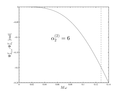
Figure 5: Difference between the full SPA tidal phase $\Psi^{T}_{k_{2,3,4}}$ obtained from a EOB waveform computed with an $A^{\rm tidal}$ including $k_{2}$, $k_{3}$ and $k_{4}$, and the tidal phase computed with $k_{2}$ only. The figure refers to a $\gamma=2$, rest-mass polytrope BNS model with ${\cal C}=0.16$ and $\bar{\alpha}_{2}^{(2)}=6$. The vertical dashed line indicates the contact frequency.

In the main text we have used the EOB approach to compute a SPA-defined, Fourier domain EOB tidal phasing, $\Psi^{T}_{\rm EOB_{SPA}}(\omega)$, where $\omega$ is the quadrupolar GW frequency so as to control the accuracy of the Fourier-domain, PN-expanded tidal phase given by Eq. (II.3) for an equal-mass binary. The analytical procedure to obtain $\Psi^{T}_{\rm EOB_{SPA}}(\omega)$ (that we shall henceforth simply denote as $\Psi^{T}(\omega)$) is described in Sec. II.2 (see in particular Eq. (20)), while the comparison with the PN-expanded tidal phasing is discussed in Sec. (II.3), in particular Figs. 1 and 2 there. The phase $\Psi^{T}(\omega)$ is computed by integrating numerically Eq. (19) starting from the frequency $\omega_{0}$ that marks the beginning of the inspiral waveform obtained when solving the EOB equations of motion numerically. This integration is done using the 2.5PN result for $\Psi^{T}_{\rm 2.5PN}$ and $d\Psi^{T}_{\rm 2.5PN}/d\omega$ as initial boundary conditions, and thus $\omega_{0}$ needs to be chosen sufficiently small (i.e., the iniitla separation is sufficiently large) so to have $Q_{\omega}^{\rm 2.5PN}\approx Q_{\omega}^{\rm EOB}$. In practice, for all compactnesses considered in Figs. 1 and 2, the initial relative separation that we use is $r_{0}=32$, which corresponds to a quadrupolar GW frequency $\omega_{0}\sim 0.111$.

A.2 Dependence of the phasing on dynamical tidal effects with $\ell>2$ and its linearity with ${\kappa_{2}^{T}}$

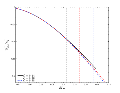
Figure 6: Approximate linearity of $\Psi^{T}_{\rm EOB}$ with respect to ${\kappa_{2}^{T}}$, with $\bar{\alpha}_{2}^{(2)}=6$. Three equal-mass (polytropic) BNS systems of compactnesses ${\cal C}=\{0.14,\,0.16,\,0.18\}$ are compared. The vertical dashed lines indicate the corresponding contact frequencies.

The use of the tidal phasing $\Psi^{T}_{\rm 2.5PN}$, Eq. (II.3) in the main text neglects by construction two physical effects that are incorporated in the EOB description, notably: (i) dynamical tidal terms with $\ell>2$ (e.g., $\ell=3$ and $\ell=4$) that enter in the definition of $A^{\rm tidal}(u)$; (ii) nonlinear effects in $\kappa_{2}^{T}$, that are present due to the resummed nature of the EOB formalism. In this Section we analyze their influence of $\Psi^{T}(\omega)$ and argue that they collectively contribute to the phasing by an amount of the order of $-0.2$ rad up to contact. On top of this contribution being small, the fact that it is negative means that any measurability analysis neglecting it is on the conservative side. Focusing on a ${\cal C}=0.16$, rest-mass, $\gamma=2$, polytrope binary, the effect of the $\ell=3$ and $\ell=4$ tidal corrections to the EOB potential is illustrated in Fig. 5. The figure shows the difference between the full $\Psi^{T}_{k_{2,3,4}}$ obtained from a EOB waveform computed retaining $k_{2}$, $k_{3}$ and $k_{4}$ in the Hamiltonian ( through $A^{\rm tidal}$), and the phase $\Psi^{T}_{k_{2}}$ computed when retaining only $k_{2}$. One sees that the phase difference at the contact frequency (indicated by the dashed vertical line) is of the order of $-0.2$ rad.

Finally, to study to what extent the dependence of $\Psi^{T}_{k_{2}}$ is linear in $k_{2}$ (and therefore ${\kappa_{2}^{T}}$), we consider three binaries with compactnesses ${\cal C}=(0.14,0.16,0.18)$. For each binary we compute the ratio $\Psi^{T}_{k_{2}}/{\kappa_{2}^{T}}$, that is displayed in Fig. 6. This figure indicates that $\Psi^{T}_{k_{2}}$ is linear in ${\kappa_{2}^{T}}$ to good approximation. From the difference ($-0.0015$ rad) between the ${\cal C}=0.18$ and ${\cal C}=0.14$ curve at $M\omega=0.1048$ (contact of ${\cal C}=0.14$ binary) one can estimate that taking into account the ${\kappa_{2}^{T}}$ would further decrease $\Psi^{T}_{k_{2}}$ by no more than $-0.3$ rad. Again, neglecting this effects means that our estimates will be on the conservative side.

Appendix B The tidal phase for a general binary at 2.5PN accuracy

In this Appendix we collect PN-expanded expressions for $Q_{\omega}^{T}$ and for $\Psi^{T}(\omega)$ for a general binary. Such a result is here expressed as a function of the PN ordering parameter $x$, of $X_{A}=M_{A}/M$ and $X_{B}=1-X_{A}$ and of the dimensionless tidal parameter $\kappa_{2}^{A}$ defined in Eq. (6). Note that this result is general, in the sense that it holds for a neutron star binary of any mass ratio, or a mixed, black-hole neutron star binary. In this latter case the tidal parameter of one of the two objects is put to zero Damour:2009vw . The equal-mass analytic expressions used in the main text are obtained as a particular case of the equations listed below, i.e., $X_{A}=X_{B}=1/2$.

In detail, the 2.5PN accurate tidal part of the $Q_{\omega}(x)$ function, $Q_{\omega}^{T}(x)$, has the structure

$$Q_{\omega}^{T}=Q_{\omega}^{A}(x)\kappa_{2}^{A}+Q_{\omega}^{B}(x)\kappa_{2}^{B}$$ (102)

where the $Q_{\omega}^{A}(x)$ contribution is written as the following PN series

$$Q_{\omega}^{A}=q^{A}_{\rm Newt}x^{5/2}\left(1+\hat{q}_{1}^{A}x+\hat{q}_{2}^{A}x^{3/2}+\hat{q}_{3}^{A}x^{2}+\hat{q}_{4}^{A}x^{5/2}\right),$$ (103)

where the coefficients read

$$q_{\rm Newt}^{A} =-\dfrac{5}{24\nu}\left(12+\dfrac{X_{A}}{X_{B}}\right)=-\dfrac{5}{24\nu}\dfrac{12-11X_{A}}{1-X_{A}},$$ (104)

$$\hat{q}_{1}^{A} =\dfrac{3179-919X_{A}-2286X_{A}^{2}+260X_{A}^{3}}{48(12-11X_{A})},$$ (105)

$$\hat{q}_{2}^{A} =-4\pi,$$ (106)

$$\hat{q}_{3}^{A} =\dfrac{1}{11X_{A}-12}\bigg{\{}\dfrac{67702048X_{A}^{5}-223216640X_{A}^{4}+337457524X_{A}^{3}-141992280X_{A}^{2}+96008669X_{A}-143740242}{338688}$$

$$+(2X_{A}-3)\beta_{2}^{22}(X_{A})+\left(\dfrac{13}{24}X-\dfrac{3}{4}X^{2}+\dfrac{X^{3}}{3}-\dfrac{1}{8}\right)\beta_{1}^{21}(X_{A})$$

$$-(1-2X_{A})(1-X_{A})^{2}\left(\dfrac{1}{1344}\beta_{1}^{31}(X_{A})+\dfrac{3645}{448}\beta_{1}^{33}(X_{A})\right)\bigg{\}},$$ (107)

$$\hat{q}_{4}^{A} =-\dfrac{\pi\left(27719-22127X_{A}+7022X_{A}^{2}-10232X_{A}^{3}\right)}{96(12-11X_{A})},$$ (108)

and we left explicit the dependence on the (yet unknown) parameters entering the tidal contribution to the waveform at fractional 2PN order, $\{\beta_{2}^{22},\,\beta_{1}^{21},\,\beta_{1}^{31},\,\beta_{1}^{33}\}$. The tidal part of the phase is then written in the following form

$$\Psi^{T}_{\rm 2.5PN}=\Psi_{A}^{T}(x)\kappa_{2}^{A}+\Psi_{B}^{T}(x)\kappa_{2}^{B},$$ (109)

where the $\Psi_{A}^{T}(x)$ contribution is given by the following PN series

$$\Psi_{A}^{T}=p^{A}_{\rm Newt}x^{5/2}\left(1+\hat{p}_{1}^{A}x+\hat{p}_{2}^{A}x^{3/2}+\hat{p}_{3}^{A}x^{2}+\hat{p}_{4}^{A}x^{5/2}\right),$$ (110)

whose coefficients read

$$p_{\rm Newt}^{A} =-\dfrac{3}{16\nu}\left(12+\dfrac{X_{A}}{X_{B}}\right)=-\dfrac{3}{16\nu}\dfrac{12-11X_{A}}{1-X_{A}},$$ (111)

$$\hat{p}_{1}^{A} =\dfrac{5\left(3179-919X_{A}-2286X_{A}^{2}+260X_{A}^{3}\right)}{672(12-11X_{A})},$$ (112)

$$\hat{p}_{2}^{A} =-\pi,$$ (113)

$$\hat{p}_{3}^{A} =\dfrac{1}{12-11X_{A}}\bigg{\{}\dfrac{39927845}{508032}-\dfrac{480043345}{9144576}X_{A}+\dfrac{9860575}{127008}X_{A}^{2}-\dfrac{421821905}{2286144}X_{A}^{3}+\dfrac{4359700}{35721}X_{A}^{4}-\dfrac{10578445}{285768}X_{A}^{5}$$

$$+\dfrac{5}{9}\left(1-\dfrac{2}{3}X_{A}\right)\beta_{2}^{22}+\dfrac{5}{648}\left(3-13X_{A}+18X_{A}^{2}-8X^{3}_{A}\right)\beta_{1}^{21}(X_{A})$$

$$+\left(1-X_{A}\right)^{2}(1-2X_{A})\left(\dfrac{5}{36288}\beta_{1}^{31}(X_{A})+\dfrac{675}{448}\beta_{1}^{33}(X_{A})\right)\bigg{\}},$$

$$\hat{p}_{4}^{A} =-\dfrac{\pi(27719-22127X_{A}+7022X_{A}^{2}-10232X_{A}^{3})}{672(12-11X_{A})}.$$ (114)

The 1PN coefficient $\hat{p}_{1}^{A}$ above was obtained in Eqs. (3.8a)-(3.8b) of Vines:2011ud . Then the relation

$$\kappa_{2}^{A}=3\dfrac{G\mu_{2}^{A}}{M^{5}}\dfrac{X_{B}}{X_{A}},$$ (115)

(and similarly with $A\leftrightarrow B$) is used so to express the tidal phase in terms of the tidal polarizability coefficients $G\mu_{2}^{A}$ and $G\mu_{2}^{B}$. By defining

$$G\bar{\mu}_{2}\equiv\frac{1}{26}\left[\left(1+12\frac{X_{B}}{X_{A}}\right)G\mu_{2}^{A}+\left(1+12\frac{X_{A}}{X_{B}}\right)G\mu_{2}^{B}\right],$$ (116)

a straightforward calculation finally yields the tidal part of the phase in the form

$$\Psi^{T}_{\rm 2.5PN}=-\dfrac{117G\bar{\mu}_{2}}{8\nu M^{5}}x^{5/2}\hat{\Psi}^{T}_{\rm 2.5PN}$$ (117)

that is the one used (with $\beta_{2}^{22}=\beta_{1}^{21}=\beta_{1}^{13}=\beta_{1}^{33}=0$) in Eq. (60) to perform the Fisher-matrix-based estimate of the measurability of $G\bar{\mu}_{2}$.

References

- (1) J. Abadie et al. (LIGO Scientific Collaboration, Virgo Collaboration), Class.Quant.Grav. 27, 173001 (2010), arXiv:1003.2480 [astro-ph.HE]
- (2) T. Damour, Gravitational radiation and the motion of compact bodies, in Gravitational Radiation, edited by N. Deruelle and T. Piran, North-Holland, Amsterdam (1983) pp. 59–144
- (3) K. Thorne and A. Campolattaro, Astrophys. J. 149, 591 (1967)
- (4) T. Hinderer, Astrophys.J. 677, 1216 (2008), arXiv:0711.2420 [astro-ph]
- (5) E. E. Flanagan and T. Hinderer, Phys.Rev. D77, 021502 (2008), arXiv:0709.1915 [astro-ph]
- (6) T. Damour and A. Nagar, Phys.Rev. D80, 084035 (2009), arXiv:0906.0096 [gr-qc]
- (7) T. Binnington and E. Poisson, Phys.Rev. D80, 084018 (2009), arXiv:0906.1366 [gr-qc]
- (8) B. Kol and M. Smolkin, JHEP 1202, 010 (2012), arXiv:1110.3764 [hep-th]
- (9) T. Hinderer, B. D. Lackey, R. N. Lang, and J. S. Read, Phys.Rev. D81, 123016 (2010), arXiv:0911.3535 [astro-ph.HE]
- (10) T. Damour, M. Soffel, and C. Xu, Phys. Rev. D 45, 1017 (1992)
- (11) T. Damour, B. R. Iyer, and B. Sathyaprakash, Phys.Rev. D63, 044023 (2001), arXiv:gr-qc/0010009 [gr-qc]
- (12) A. Buonanno and T. Damour, Phys. Rev. D59, 084006 (1999)
- (13) A. Buonanno and T. Damour, Phys. Rev. D62, 064015 (2000)
- (14) T. Damour, P. Jaranowski, and G. Schaefer, Phys. Rev. D62, 084011 (2000)
- (15) T. Damour, Phys. Rev. D64, 124013 (2001)
- (16) T. Damour, B. R. Iyer, and A. Nagar, Phys. Rev. D79, 064004 (2009)
- (17) T. Damour and A. Nagar, The Effective One Body description of the Two-Body problem, in Mass and Motion in General Relativity, edited by L. Blanchet, A. Spallicci and B. Whiting, Springer, Dordrecht (2011) pp. 211–252, arXiv:0906.1769 [gr-qc]
- (18) T. Damour and A. Nagar, Phys.Rev. D81, 084016 (2010), arXiv:0911.5041 [gr-qc]
- (19) T. Damour and A. Nagar, Phys. Rev. D79, 081503 (2009)
- (20) Y. Pan, A. Buonanno, L. T. Buchman, T. Chu, L. E. Kidder, et al., Phys.Rev. D81, 084041 (2010), arXiv:0912.3466 [gr-qc]
- (21) Y. Pan, A. Buonanno, M. Boyle, L. T. Buchman, L. E. Kidder, et al., Phys.Rev. D84, 124052 (2011), 26 pages, 25 figures, published Phys. Rev. D version, arXiv:1106.1021 [gr-qc]
- (22) L. Baiotti, T. Damour, B. Giacomazzo, A. Nagar, and L. Rezzolla, Phys.Rev.Lett. 105, 261101 (2010), arXiv:1009.0521 [gr-qc]
- (23) L. Baiotti, T. Damour, B. Giacomazzo, A. Nagar, and L. Rezzolla, Phys.Rev. D84, 024017 (2011), arXiv:1103.3874 [gr-qc]
- (24) D. Bini, T. Damour, and G. Faye(2012), arXiv:1202.3565 [gr-qc]
- (25) P. Demorest, T. Pennucci, S. Ransom, M. Roberts, and J. Hessels, Nature 467, 1081 (2010), arXiv:1010.5788 [astro-ph.HE]
- (26) F. Pannarale, L. Rezzolla, F. Ohme, and J. S. Read, Phys.Rev. D84, 104017 (2011), arXiv:1103.3526 [astro-ph.HE]
- (27) B. D. Lackey, K. Kyutoku, M. Shibata, P. R. Brady, and J. L. Friedman, Phys.Rev. D85, 044061 (2012), 21 pages, 14 figures, submitted to PRD, arXiv:1109.3402 [astro-ph.HE]
- (28) J. E. Vines and E. E. Flanagan(2010), arXiv:1009.4919 [gr-qc]
- (29) T. Damour, B. R. Iyer, and B. Sathyaprakash, Phys.Rev. D62, 084036 (2000), arXiv:gr-qc/0001023 [gr-qc]
- (30) J. Vines, E. E. Flanagan, and T. Hinderer, Phys.Rev. D83, 084051 (2011), arXiv:1101.1673 [gr-qc]
- (31) C. Cutler and E. E. Flanagan, Phys.Rev. D49, 2658 (1994), arXiv:gr-qc/9402014 [gr-qc]
- (32) E. Poisson and C. M. Will, Phys.Rev. D52, 848 (1995), arXiv:gr-qc/9502040 [gr-qc]
- (33) D. Shoemaker https://dcc.ligo.org/cgi-bin/DocDB/ShowDocument?docid=2974
- (34) T. Damour, B. R. Iyer, and B. Sathyaprakash, Phys.Rev. D66, 027502 (2002), arXiv:gr-qc/0207021 [gr-qc]
- (35) A. Buonanno, B. Iyer, E. Ochsner, Y. Pan, and B. Sathyaprakash, Phys.Rev. D80, 084043 (2009), arXiv:0907.0700 [gr-qc]
- (36) L. Blanchet, T. Damour, B. R. Iyer, C. M. Will, and A. Wiseman, Phys.Rev.Lett. 74, 3515 (1995)
- (37) D. R. Lorimer, Living Rev. Rel. 11, 8 (2008), arXiv:0811.0762 [astro-ph]
- (38) M. Bejger, T. Bulik, and P. Haensel, Mon. Not. Roy. Astron. Soc. 364, 635 (2005), arXiv:astro-ph/0508105
- (39) I. Morrison, T. W. Baumgarte, S. Shapiro, and V. Pandharipande, Astrophys.J. 617, L135 (2004), arXiv:astro-ph/0411353 [astro-ph]
- (40) H. Mueller and B. D. Serot, Nucl.Phys. A606, 508 (1996), arXiv:nucl-th/9603037 [nucl-th]
- (41) A. Akmal, V. R. Pandharipande, and D. G. Ravenhall, Phys. Rev. C 58, 1804 (Sep 1998)
- (42) N. Glendenning, Astrophys.J. 293, 470 (1985)
- (43) N. Chamel, A. Fantina, J. Pearson, and S. Goriely, Phys.Rev. C84, 062802 (2011), arXiv:1112.2878 [nucl-th]
- (44) S. Bernuzzi and A. Nagar, Phys.Rev. D78, 024024 (2008), arXiv:0803.3804 [gr-qc]
- (45) T. Bulik, D. Gondek-Rosinska, and K. Belczynski, Mon.Not.Roy.Astron.Soc. 352, 1372 (2004), arXiv:astro-ph/0310544 [astro-ph]
- (46) L. Baiotti, B. Giacomazzo, and L. Rezzolla, Phys.Rev. D78, 084033 (2008), arXiv:0804.0594 [gr-qc]
- (47) S. Bernuzzi, A. Nagar, and A. Zenginoglu, Phys.Rev. D83, 064010 (2011), arXiv:1012.2456 [gr-qc]
- (48) K. Hotokezaka, K. Kyutoku, H. Okawa, M. Shibata, and K. Kiuchi, Phys.Rev. D83, 124008 (2011), arXiv:1105.4370 [astro-ph.HE]
- (49) A. Bauswein and H.-T. Janka, Phys.Rev.Lett. 108, 011101 (2012), arXiv:1106.1616 [astro-ph.SR]
- (50) J. S. Read, B. D. Lackey, B. J. Owen, and J. L. Friedman, Phys.Rev. D79, 124032 (2009), arXiv:0812.2163 [astro-ph]
- (51) L. Blanchet and T. Damour, Annales Poincare Phys.Theor. 50, 377 (1989)
- (52) L. Blanchet and T. Damour, Phys.Rev. D46, 4304 (1992)
- (53) L. Blanchet, Phys.Rev. D51, 2559 (1995), arXiv:gr-qc/9501030 [gr-qc]
- (54) T. Damour and A. Nagar, Phys. Rev. D76, 064028 (2007), arXiv:0705.2519 [gr-qc]
- (55) T. Damour and A. Nagar, Phys.Rev. D77, 024043 (2008), arXiv:0711.2628 [gr-qc]
- (56) T. Damour and A. Gopakumar, Phys. Rev. D73, 124006 (2006), arXiv:gr-qc/0602117
- (57) R. Fujita and B. R. Iyer, Phys. Rev. D82, 044051 (2010), arXiv:1005.2266 [gr-qc]