Constraint on compactification scale via recently observed baryonic $\Lambda_{b}\rightarrow\Lambda\ell^{+}\ell^{-}$ channel and analysis of the $\Sigma_{b}\rightarrow\Sigma\ell^{+}\ell^{-}$ transition in SM and UED scenario

We obtain a lower limit on the compactification scale of extra dimension via comparison of the branching ratio in the baryonic $\Lambda_{b}\rightarrow\Lambda\mu^{+}\mu^{-}$ decay channel recently measured by CDF collaboration and our previous theoretical study. We also use the newly available form factors calculated via light cone QCD sum rules in full theory to analyze the flavour changing neutral current process of the $\Sigma_{b}\rightarrow\Sigma\ell^{+}\ell^{-}$ in universal extra dimension scenario in the presence of a single extra compact dimension. We calculate various physical quantities like branching ratio, forward-backward asymmetry, baryon polarizations and double lepton polarization asymmetries defining the decay channel under consideration. We also compare the obtained predictions with those of the standard model.

PACS number(s): 12.60-i, 13.30.-a, 13.30.Ce, 14.20.Mr

1 Introduction

The CDF Collaboration at Fermilab has recently reported the first observation of the baryonic flavour changing neutral current (FCNC) decay $\Lambda_{b}\rightarrow\Lambda\mu^{+}\mu^{-}$ with $24$ signal events and a statistical significance of $5.8~{}\sigma$ [1]. This event as the first FCNC observation in baryonic sector has stimulated both experimental and theoretical studied in this area. The LHCb collaboration at CERN has also started to study this decay channel [2]. Comparison of the theoretical and phenomenological predictions on related physical observables with experimental data can help us get valuable information not only about the internal structure of the participating particles, strong interaction and other parameters of the standard model (SM) but about the new physics effects. Such comparison leads to put constraints on the parameters existing in many new physics scenarios beyond the SM (BSM).

The FCNC transitions are very important frameworks to indirectly search for extra dimensions and Kaluza Klein (KK) particles as new physics effects. In the past, putting constraints on the compactification scale, $1/R$ of extra dimensions and mass of KK modes was passable only via comparison of the experimental data on physical observables with theoretical predictions in mesonic sector. By the above mentioned developments, now, it is possible to get knowledge on these parameters also in FCNC baryonic decay channels. Our first task in the present study is to put constraint on the compactification scale of extra dimension by comparing the experimental data on the branching fraction of the $\Lambda_{b}\rightarrow\Lambda\mu^{+}\mu^{-}$ and our theoretical prediction [3] in universal extra dimension (UED) framework with a single extra dimension called Applequist-Cheng-Dobrescu (ACD) model (For more information about the model and idea of extra dimension (ED) see [4, 5, 6, 7, 8, 9, 10, 11]). Note that this decay channel was studied in detail in SM in [12].

In the second and main part of the present study, we work out the other baryonic FCNC $\Sigma_{b}\rightarrow\Sigma\ell^{+}\ell^{-}$ transition in the context of UED may will be in agenda of experiments in future. We use the form factors, very recently calculated via light cone QCD sum rules in full theory [13], as the main ingredients in this channel. The order of branching ratio on this channel reported in [13] shows that this decay channel is also accessible at LHC. We use the transition form factors enrolled to the low energy effective Hamiltonian to calculate many physical observables related to the decay channel under consideration. Particularly, we evaluate the branching ratio, forward-backward asymmetry, baryon polarizations and double lepton polarization asymmetries both in the SM and UED and compare our results on the considered physical quantities obtained via these two models. The UED model has also been applied to many channels mainly in mesonic sector (see for instance [14, 15, 17, 18, 19, 16, 20, 21, 22, 23, 24, 25, 26, 27, 28] and references therein).

The layout of the article is as follows. In next section, we find a lower limit on the compactification scale via comparing the experimental result on the branching ratio of the $\Lambda_{b}\rightarrow\Lambda\mu^{+}\mu^{-}$ and theoretical prediction. In section 3, we evaluate the $\Sigma_{b}\rightarrow\Sigma\ell^{+}\ell^{-}$ transition in UED model and calculate the corresponding physical quantities. In this section, we also numerically analyze the observables defining the transition under consideration and compare the obtained results with SM predictions. Last section encompasses our discussions and conclusions.

2 Constraint on the Compactification Factor via $\Lambda_{b}\rightarrow\Lambda\mu^{+}\mu^{-}$ Decay Channel

In ED models [6, 7, 8, 9, 10, 11], gravity can travel in the higher dimensional bulk. This give rise to KK towers of massive spin-2 graviton excitations or KK gravitons whose possible destination can be a tour along a circle of radius $R$ called size of the extra dimension and return to where they began. The mass difference between subsequent KK particles is of order $1/R$. In UED model, the SM fields (both gauge bosons and fermions) are also allowed to propagate in the extra dimensions [4, 5]. As a result of interactions among the SM and KK particles, the Wilson coefficients entering effective Hamiltonian become functions of compactification scale $1/R$ (we will come back to this point in next section). Hence, it will be of great importance to put constraint on this factor.

The lower bound of compactification factor has been put mainly comparing the experimental data with theoretical calculations in mesonic channel, electroweak precision tests and some cosmological constraints. Analysis of the $B\rightarrow X_{s}\gamma$ decay channel and anomalous magnetic moment depict that when $1/R\geq 300~{}GeV$, the experimental data are in good agreements with the UED model predictions [29]. In [4, 5], based on also the electroweak precision tests, it has been found that the lower limit for compactification scale is $250~{}GeV$ when $M_{Higgs}\geq 250~{}GeV$ denoting larger KK contributions to the low energy FCNC transitions, and $300~{}GeV$ when $M_{Higgs}\leq 250~{}GeV$. According to [30] and [31], again the electroweak precision measurements as well as some cosmological constraints give rise to $500~{}GeV$ for the lower limit on compactification scale. Contributing the leading order (LO) and next-to-next-to-leading order (NNLO) corrections due to the exchange of KK modes also to the ${\cal B}(B\rightarrow X_{s}\gamma)$ transition in [32] has lead to $600~{}GeV$ as lower bound on $1/R$. Moreover, the ATLAS collaboration at CERN has set a $600~{}GeV$ on the lower bound of $1/R$, for values of the compression scale between $2$ and $40$, implying $730~{}GeV$ for lower bound of the mass of the KK gluons [33]. However, very recently, the authors of [34] have found that the theoretical result on ${\cal B}(B\rightarrow K\eta\gamma)$ matches with experimental data if $1/R\gtrsim 250~{}GeV$ as far as they consider a single UED. This is lower than the bound provided by other processes [35]. But when they add the second dimension (with 2 UEDs), they find $\simeq 400~{}GeV$ for the lower limit of the compactification factor.

As we previously mentioned, now we have the first experimental measurement on the branching ratio of $\Lambda_{b}\rightarrow\Lambda\mu^{+}\mu^{-}$, i.e., $B(\Lambda_{b}\rightarrow\Lambda\mu^{+}\mu^{-})=[1.73\pm 0.42$(stat)$\pm 0.55$(syst)$]\times 10^{-6}$ [1]. This gives a possibility to obtain a lower bound on the compactification scale $1/R$ in baryonic sector by comparison between this experimental result and our previous theoretical prediction [3] but only when a single UED is considered. The process $B\rightarrow K\eta\gamma$ is described by only one Wilson coefficient $C_{7}^{eff}$ whose explicit expression is available in UED model with 2 EDs. However, in our case the Effective Hamiltonian describing the $\Lambda_{b}\rightarrow\Lambda\mu^{+}\mu^{-}$ channel contains additional coefficients, $C_{9}^{eff}$ and $C_{10}$ (for details see next section) whose values have not been known in UED with 2 EDs yet. Hence, it is now possible to find a lower limit on $1/R$ via baryonic FCNC $\Lambda_{b}\rightarrow\Lambda\mu^{+}\mu^{-}$ process in UED model with a single ED. The comparison is made in Figure 1 where we have considered the errors of form factors and uncertainties of other input parameters in theoretical calculations.

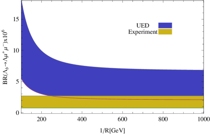
Figure 1: Comparison between the experimental result [1] and theoretical prediction [3] on the branching ratio of $\Lambda_{b}\rightarrow\Lambda\mu^{+}\mu^{-}$ channel.

From this figure, we obtain an approximately $250~{}GeV$ for the lower bound of $1/R$ which is in a good consistency with the result of [34] when only one UED is taken into account. To improve our result, one should take the effects of second ED in the process under consideration and this will be possible when the explicit form of additional Wilson coefficients $C_{9}^{eff}$ and $C_{10}$ are known.

3 The $\Sigma_{b}\rightarrow\Sigma\ell^{+}\ell^{-}$ Transition in UED

3.1 The Effective Hamiltonian and Transition Matrix Elements

The FCNC transition of the $\Sigma_{b}\rightarrow\Sigma\ell^{+}\ell^{-}$ proceeds via loop-level $b\rightarrow sl^{+}l^{-}$ transition whose effective Hamiltonian can be written as

$${\cal H}^{eff} = {G_{F}\alpha_{em}V_{tb}V_{ts}^{\ast}\over 2\sqrt{2}\pi}\Bigg{[}C_{9}^{eff}\bar{s}\gamma_{\mu}(1-\gamma_{5})b\,\bar{\ell}\gamma^{\mu}\ell+C_{10}\bar{s}\gamma_{\mu}(1-\gamma_{5})b\,\bar{\ell}\gamma^{\mu}\gamma_{5}\ell$$ (3.1)

$$- 2m_{b}C_{7}^{eff}{1\over q^{2}}\bar{s}i\sigma_{\mu\nu}(1+\gamma_{5})b\,\bar{\ell}\gamma^{\mu}\ell\Bigg{]}~{},$$

where $G_{F}$ is the Fermi weak coupling constant, $V_{ij}$ are the Cabibbo-Kobayashi-Maskawa (CKM) matrix elements, $\alpha_{em}$ is the fine structure constant; and $C_{7}^{eff}$, $C_{9}^{eff}$ and $C_{10}$ are Wilson coefficients. The transition amplitude of hadronic decay channel under consideration is defined as

$${\cal M}=\langle\Sigma(p)\mid{\cal H}^{eff}\mid\Sigma_{b}(p+q)\rangle.$$ (3.2)

As a result of this procedure, we get the following transition matrix elements parameterized in terms of transition form factors:

$$\langle\Sigma(p)\mid\bar{s}\gamma_{\mu}(1-\gamma_{5})b\mid\Sigma_{b}(p+q)\rangle\!\!\! = \!\!\!\bar{u}_{\Sigma}(p)\Big{[}\gamma_{\mu}f_{1}(q^{2})+{i}\sigma_{\mu\nu}q^{\nu}f_{2}(q^{2})+q^{\mu}f_{3}(q^{2})$$

$$- \!\!\!\gamma_{\mu}\gamma_{5}g_{1}(q^{2})-{i}\sigma_{\mu\nu}\gamma_{5}q^{\nu}g_{2}(q^{2})-q^{\mu}\gamma_{5}g_{3}(q^{2})\vphantom{\int_{0}^{x_{2}}}\Big{]}u_{\Sigma_{b}}(p+q)~{},$$

and,

$$\langle\Sigma(p)\mid\bar{s}i\sigma_{\mu\nu}q^{\nu}(1+\gamma_{5})b\mid\Sigma_{b}(p+q)\rangle\!\!\! = \!\!\!\bar{u}_{\Sigma}(p)\Big{[}\gamma_{\mu}f_{1}^{T}(q^{2})+{i}\sigma_{\mu\nu}q^{\nu}f_{2}^{T}(q^{2})+q^{\mu}f_{3}^{T}(q^{2})$$

$$+ \!\!\!\gamma_{\mu}\gamma_{5}g_{1}^{T}(q^{2})+{i}\sigma_{\mu\nu}\gamma_{5}q^{\nu}g_{2}^{T}(q^{2})+q^{\mu}\gamma_{5}g_{3}^{T}(q^{2})\vphantom{\int_{0}^{x_{2}}}\Big{]}u_{\Sigma_{b}}(p+q)~{},$$

where $f^{(T)}_{i}$ and $g^{(T)}_{i}$ ($i$ runs from $1$ to $3$) are form factors; and $u_{\Sigma_{b}}$ and $u_{\Sigma}$ are spinors of $\Sigma_{b}$ and $\Sigma$ baryons, respectively. These form factors as the main inputs in analysis of the $\Sigma_{b}\rightarrow\Sigma\ell^{+}\ell^{-}$ have been very recently calculated in full QCD via light cone QCD sum rules in [13]. By full QCD, we mean full theory of QCD without any approximation like heavy quark effective theory (HQET) limit. The fit function of transition form factors is given as [13]:

$$f^{(T)}_{i}(q^{2})[g^{(T)}_{i}(q^{2})]=\frac{a}{(1-\frac{q^{2}}{m_{fit}^{2}})}+\frac{b}{(1-\frac{q^{2}}{m_{fit}^{2}})^{2}},$$ (3.5)

where the fit parameters $a$, $b$, and $m_{fit}$ are presented in Table 1.

$$\begin{array}[]{|c|c|c|c|c|c|}\hline\cr\hline\cr&\mbox{a}&\mbox{b}&m_{fit}&q^{2}=0\\ \hline\cr f_{1}&-0.035&0.13&5.1&0.095\pm 0.017\\ f_{2}&0.026&-0.081&5.2&-0.055\pm 0.012\\ f_{3}&0.013&-0.065&5.3&-0.052\pm 0.016\\ g_{1}&-0.031&0.15&5.3&0.12\pm 0.03\\ g_{2}&0.015&-0.040&5.3&-0.025\pm 0.008\\ g_{3}&0.012&-0.047&5.4&-0.035\pm 0.009\\ f_{1}^{T}&1.0&-1.0&5.4&0.0\pm 0.0\\ f_{2}^{T}&-0.29&0.42&5.4&0.13\pm 0.04\\ f_{3}^{T}&-0.24&0.41&5.4&0.17\pm 0.05\\ g_{1}^{T}&0.45&-0.46&5.4&-0.010\pm 0.003\\ g_{2}^{T}&0.031&0.055&5.4&0.086\pm 0.024\\ g_{3}^{T}&-0.011&-0.18&5.4&-0.19\pm 0.06\\ \hline\cr\hline\cr\end{array}$$

Table 1: Parameters appearing in the fit function of the form factors, $f_{1}$, $f_{2}$, $f_{3}$, $g_{1}$, $g_{2}$, $g_{3}$, $f^{T}_{1}$, $f^{T}_{2}$, $f^{T}_{3}$, $g^{T}_{1}$, $g^{T}_{2}$ and $g^{T}_{3}$ in full theory for $\Sigma_{b}\rightarrow\Sigma\ell^{+}\ell^{-}$ together with the values of the form factors at $q^{2}=0$ [13].

After the above comments about the amplitude and transition matrix elements, we go on to discuss the source of main differences between UED and SM models. Such differences belong to the Wilson coefficients entered the effective Hamiltonian. As we previously mentioned the KK particles in UED models interact with themselves as well as the SM particles in the bulk, giving rise to modifications in the SM versions of the Wilson coefficients although the form of effective Hamiltonian remain unchanged. Each Wilson coefficient in UED scenario is defined in terms of a SM part $F_{0}(x_{t})$ and extra periodic functions $F_{n}(x_{t},x_{n})$ coming from new interactions, i.e.,

$$F(x_{t},1/R)=F_{0}(x_{t})+\sum_{n=1}^{\infty}F_{n}(x_{t},x_{n}).$$ (3.6)

Here, $x_{t}=\frac{m_{t}^{2}}{M_{W}^{2}}$, $x_{n}=\displaystyle{m_{n}^{2}\over m_{W}^{2}}$, and $m_{n}=\displaystyle{n\over R}$. Also, $m_{t}$, $M_{W}$ and $m_{n}$ are masses of the top quark, $W$ boson and KK particles (non-zero modes), respectively. The Wilson coefficients $C_{7}^{eff}$, $C_{9}^{eff}$ and $C_{10}$ have been calculated in UED in the presence of a single ED and SM models in [14, 15, 38, 36, 37]. The $C_{9}^{eff}$ which is a function of $\hat{s}^{\prime}=\frac{q^{2}}{m_{b}^{2}}$ with $4m_{l}^{2}\leq q^{2}\leq(m_{\Sigma_{b}}-m_{\Sigma})^{2}$ and compactification scale, is given as

$$C_{9}^{eff}(\hat{s}^{\prime},1/R) = C_{9}^{NDR}(1/R)\eta(\hat{s}^{\prime})+h(z,\hat{s}^{\prime})\left(3C_{1}+C_{2}+3C_{3}+C_{4}+3C_{5}+C_{6}\right)$$ (3.7)

$$-\frac{1}{2}h(1,\hat{s}^{\prime})\left(4C_{3}+4C_{4}+3C_{5}+C_{6}\right)$$

$$-\frac{1}{2}h(0,\hat{s}^{\prime})\left(C_{3}+3C_{4}\right)+\frac{2}{9}\left(3C_{3}+C_{4}+3C_{5}+C_{6}\right),$$

where

$$\eta(\hat{s}^{\prime}) = 1+\frac{\alpha_{s}(\mu_{b})}{\pi}\,\omega(\hat{s}^{\prime}),$$ (3.8)

with

$$\omega(\hat{s}^{\prime}) = -\frac{2}{9}\pi^{2}-\frac{4}{3}\mbox{Li}_{2}(\hat{s}^{\prime})-\frac{2}{3}\ln\hat{s}^{\prime}\ln(1-\hat{s}^{\prime})-\frac{5+4\hat{s}^{\prime}}{3(1+2\hat{s}^{\prime})}\ln(1-\hat{s}^{\prime})-$$ (3.9)

$$\frac{2\hat{s}^{\prime}(1+\hat{s}^{\prime})(1-2\hat{s}^{\prime})}{3(1-\hat{s}^{\prime})^{2}(1+2\hat{s}^{\prime})}\ln\hat{s}^{\prime}+\frac{5+9\hat{s}^{\prime}-6\hat{s}^{\prime 2}}{6(1-\hat{s}^{\prime})(1+2\hat{s}^{\prime})},$$

and

$$\alpha_{s}(x)=\frac{\alpha_{s}(m_{Z})}{1-\beta_{0}\frac{\alpha_{s}(m_{Z})}{2\pi}\ln(\frac{m_{Z}}{x})}.$$ (3.10)

Here, $\alpha_{s}(m_{Z})=0.118$ and $\beta_{0}=\frac{23}{3}$. At $\mu_{b}$ scale we have

$$C_{j}=\sum_{i=1}^{8}k_{ji}\eta^{a_{i}}\qquad(j=1,...6)\vspace{0.2cm},$$ (3.11)

where

$$\eta\!\!\! = \!\!\!\frac{\alpha_{s}(\mu_{W})}{\alpha_{s}(\mu_{b})}~{},$$ (3.12)

$$\frac{}{}\begin{array}[]{rrrrrrrrrl}a_{i}=(\!\!&\frac{14}{23},&\frac{16}{23},&\frac{6}{23},&-\frac{12}{23},&0.4086,&-0.4230,&-0.8994,&0.1456&\!\!)\vspace{0.1cm},\end{array}$$ (3.13)

and

$$\frac{}{}\begin{array}[]{rrrrrrrrrl}k_{1i}=(\!\!&0,&0,&\frac{1}{2},&-\frac{1}{2},&0,&0,&0,&0&\!\!),\vspace{0.1cm}\\ k_{2i}=(\!\!&0,&0,&\frac{1}{2},&\frac{1}{2},&0,&0,&0,&0&\!\!),\vspace{0.1cm}\\ k_{3i}=(\!\!&0,&0,&-\frac{1}{14},&\frac{1}{6},&0.0510,&-0.1403,&-0.0113,&0.0054&\!\!),\vspace{0.1cm}\\ k_{4i}=(\!\!&0,&0,&-\frac{1}{14},&-\frac{1}{6},&0.0984,&0.1214,&0.0156,&0.0026&\!\!),\vspace{0.1cm}\\ k_{5i}=(\!\!&0,&0,&0,&0,&-0.0397,&0.0117,&-0.0025,&0.0304&\!\!),\vspace{0.1cm}\\ k_{6i}=(\!\!&0,&0,&0,&0,&0.0335,&0.0239,&-0.0462,&-0.0112&\!\!).\vspace{0.1cm}\\ \end{array}$$ (3.14)

The function, $h(y,\hat{s}^{\prime})$ is given as

$$h(y,\hat{s}^{\prime}) = -\frac{8}{9}\ln\frac{m_{b}}{\mu_{b}}-\frac{8}{9}\ln y+\frac{8}{27}+\frac{4}{9}x$$ (3.17)

$$-\frac{2}{9}(2+x)|1-x|^{1/2}\left\{\begin{array}[]{ll}\left(\ln\left|\frac{\sqrt{1-x}+1}{\sqrt{1-x}-1}\right|-i\pi\right),&\mbox{for }x\equiv\frac{4z^{2}}{\hat{s}^{\prime}}<1\\ 2\arctan\frac{1}{\sqrt{x-1}},&\mbox{for }x\equiv\frac{4z^{2}}{\hat{s}^{\prime}}>1,\end{array}\right.$$

where $y=1$ or $y=z=\frac{m_{c}}{m_{b}}$ and,

$$h(0,\hat{s}^{\prime}) = \frac{8}{27}-\frac{8}{9}\ln\frac{m_{b}}{\mu_{b}}-\frac{4}{9}\ln\hat{s}^{\prime}+\frac{4}{9}i\pi.$$ (3.19)

The $C_{9}^{NDR}(1/R)$ in (3.7) is expressed as

$$C_{9}^{NDR}(1/R) = P_{0}^{NDR}+\frac{Y(x_{t},1/R)}{\sin^{2}\theta_{W}}-4Z(x_{t},1/R)+P_{E}E(x_{t},1/R),$$ (3.20)

where $P_{0}^{NDR}=2.60\pm 0.25$, $\sin^{2}\theta_{W}=0.23$ [36, 37] and NDR is the abbreviation, used for naive dimensional regularization. Due to smallness of the $P_{E}$, the last term in (3.20) is neglected and remaining functions, $Y(x_{t},1/R)$ and $Z(x_{t},1/R)$ are defined in the following way:

$$Y(x_{t},1/R)\!\!\! = \!\!\!Y_{0}(x_{t})+\sum_{n=1}^{\infty}C_{n}(x_{t},x_{n})~{},$$ (3.21)

where

$$Y_{0}(x_{t})\!\!\! = \!\!\!\frac{x_{t}}{8}\left[\frac{x_{t}-4}{x_{t}-1}+\frac{3x_{t}}{(x_{t}-1)^{2}}\ln x_{t}\right]~{},$$ (3.22)

and

$$\sum_{n=1}^{\infty}C_{n}(x_{t},x_{n})=\frac{x_{t}(7-x_{t})}{16(x_{t}-1)}-\frac{\pi m_{W}Rx_{t}}{16(x_{t}-1)^{2}}\left[3(1+x_{t})J(R,-1/2)+(x_{t}-7)J(R,1/2)\right]~{}.$$

with

$$J(R,\alpha)=\int_{0}^{1}dy\,y^{\alpha}\left[\coth(\pi m_{W}R\sqrt{y})-x_{t}^{1+\alpha}\coth(\pi m_{t}R\sqrt{y})\right]~{}.$$ (3.24)

The $Z(x_{t},1/R)$ is defined as

$$Z(x_{t},1/R)\!\!\! = \!\!\!Z_{0}(x_{t})+\sum_{n=1}^{\infty}C_{n}(x_{t},x_{n})~{},$$ (3.25)

where

$$Z_{0}(x_{t})\!\!\! = \!\!\!\frac{18x_{t}^{4}-163x_{t}^{3}+259x_{t}^{2}-108x_{t}}{144(x_{t}-1)^{3}}+\left[\frac{32x_{t}^{4}-38x_{t}^{3}-15x_{t}^{2}+18x_{t}}{72(x_{t}-1)^{4}}-\frac{1}{9}\right]\ln x_{t}.$$

The Wilson coefficient, $C_{10}$ can be written as

$$C_{10}(1/R)=-\frac{Y(x_{t},1/R)}{\sin^{2}\theta_{W}}~{}.$$ (3.27)

Finally, in leading log approximation, the Wilson coefficient $C_{7}^{eff}(1/R)$ is given as

$$C_{7}^{eff}(\mu_{b},1/R)\!\!\! = \!\!\!\eta^{\frac{16}{23}}C_{7}(\mu_{W},1/R)+\frac{8}{3}\left(\eta^{\frac{14}{23}}-\eta^{\frac{16}{23}}\right)C_{8}(\mu_{W},1/R)+C_{2}(\mu_{W})\sum_{i=1}^{8}h_{i}\eta^{a_{i}}~{},$$

where

$$C_{2}(\mu_{W})=1~{},~{}~{}C_{7}(\mu_{W},1/R)=-\frac{1}{2}D^{\prime}(x_{t},1/R)~{},~{}~{}C_{8}(\mu_{W},1/R)=-\frac{1}{2}E^{\prime}(x_{t},1/R)~{}.$$ (3.29)

The functions, $D^{\prime}(x_{t},1/R)$ and $E^{\prime}(x_{t},1/R)$ are given as:

$$D^{\prime}(x_{t},1/R)=D^{\prime}_{0}(x_{t})+\sum_{n=1}^{\infty}D^{\prime}_{n}(x_{t},x_{n}),~{}~{}~{}~{}~{}E^{\prime}(x_{t},1/R)=E^{\prime}_{0}(x_{t})+\sum_{n=1}^{\infty}E^{\prime}_{n}(x_{t},x_{n})~{},$$ (3.30)

where $D^{\prime}_{0}(x_{t})$ and $E^{\prime}_{0}(x_{t})$ have expresions

$$D^{\prime}_{0}(x_{t})\!\!\! = \!\!\!-\frac{(8x_{t}^{3}+5x_{t}^{2}-7x_{t})}{12(1-x_{t})^{3}}+\frac{x_{t}^{2}(2-3x_{t})}{2(1-x_{t})^{4}}\ln x_{t}~{},$$ (3.31)

$$E^{\prime}_{0}(x_{t})\!\!\! = \!\!\!-\frac{x_{t}(x_{t}^{2}-5x_{t}-2)}{4(1-x_{t})^{3}}+\frac{3x_{t}^{2}}{2(1-x_{t})^{4}}\ln x_{t}~{},$$ (3.32)

and the functions representing KK contributions are,

$$\sum_{n=1}^{\infty}D^{\prime}_{n}(x_{t},x_{n})\!\!\! = \!\!\!\frac{x_{t}[37-x_{t}(44+17x_{t})]}{72(x_{t}-1)^{3}}$$

$$+ \!\!\!\frac{\pi m_{W}R}{12}\Bigg{[}\int_{0}^{1}dy\,(2y^{1/2}+7y^{3/2}+3y^{5/2})\,\coth(\pi m_{W}R\sqrt{y})$$

$$- \!\!\!\frac{x_{t}(2-3x_{t})(1+3x_{t})}{(x_{t}-1)^{4}}J(R,-1/2)$$

$$- \!\!\!\frac{1}{(x_{t}-1)^{4}}\{x_{t}(1+3x_{t})+(2-3x_{t})[1-(10-x_{t})x_{t}]\}J(R,1/2)$$

$$- \!\!\!\frac{1}{(x_{t}-1)^{4}}[(2-3x_{t})(3+x_{t})+1-(10-x_{t})x_{t}]J(R,3/2)$$

$$- \!\!\!\frac{(3+x_{t})}{(x_{t}-1)^{4}}J(R,5/2)\Bigg{]}~{},$$

$$\sum_{n=1}^{\infty}E^{\prime}_{n}(x_{t},x_{n})\!\!\! = \!\!\!\frac{x_{t}[17+(8-x_{t})x_{t}]}{24(x_{t}-1)^{3}}$$ (3.34)

$$+ \!\!\!\frac{\pi m_{W}R}{4}\Bigg{[}\int_{0}^{1}dy\,(y^{1/2}+2y^{3/2}-3y^{5/2})\,\coth(\pi m_{W}R\sqrt{y})$$

$$- \!\!\!{x_{t}(1+3x_{t})\over(x_{t}-1)^{4}}J(R,-1/2)$$

$$+ \!\!\!\frac{1}{(x_{t}-1)^{4}}[x_{t}(1+3x_{t})-1+(10-x_{t})x_{t}]J(R,1/2)$$

$$- \!\!\!\frac{1}{(x_{t}-1)^{4}}[(3+x_{t})-1+(10-x_{t})x_{t})]J(R,3/2)$$

$$+ \!\!\!{(3+x_{t})\over(x_{t}-1)^{4}}J(R,5/2)\Bigg{]}~{}.$$

The coefficients $h_{i}$ in Eq.(3.1) are given by the following values [36, 37]:

$$\frac{}{}\begin{array}[]{rrrrrrrrrl}h_{i}=(\!\!&2.2996,&-1.0880,&-\frac{3}{7},&-\frac{1}{14},&-0.6494,&-0.0380,&-0.0186,&-0.0057&\!\!).\end{array}$$ (3.35)

3.2 Branching Ratio

Having the decay amplitude in Eq.(3.2), the $1/R$-dependent double differential decay rate is obtained as [21, 39, 40]:

$$\frac{d^{2}\Gamma}{d\hat{s}dz}(z,\hat{s},1/R)=\frac{G_{F}^{2}\alpha^{2}_{em}m_{\Sigma_{b}}}{16384\pi^{5}}|V_{tb}V_{ts}^{*}|^{2}v\sqrt{\lambda}\,\Bigg{[}{\cal T}_{0}(\hat{s},1/R)+{\cal T}_{1}(\hat{s},1/R)z+{\cal T}_{2}(\hat{s},1/R)z^{2}\Bigg{]}~{},$$

(3.36)

where $\hat{s}=\frac{q^{2}}{m_{\Sigma_{b}}^{2}}$, $z=\cos\theta$ and $\theta$ is the angle between momenta of lepton $l^{+}$ and $\Sigma_{b}$ in the center of mass of leptons. Here, $\lambda=\lambda(1,r,\hat{s})=(1-r-\hat{s})^{2}-4r\hat{s}$ is the usual triangle function, $v=\sqrt{1-\frac{4m_{\ell}^{2}}{q^{2}}}$ is the lepton velocity and $r=m^{2}_{\Sigma}/m^{2}_{\Sigma_{b}}$. The ${\cal T}_{i}(\hat{s},1/R)$ functions are given as:

$${\cal T}_{0}(\hat{s},1/R)\!\!\! = \!\!\!32m_{\ell}^{2}m_{\Sigma_{b}}^{4}\hat{s}(1+r-\hat{s})\left(\left|D_{3}\right|^{2}+\left|E_{3}\right|^{2}\right)$$

$$+ \!\!\!64m_{\ell}^{2}m_{\Sigma_{b}}^{3}(1-r-\hat{s})\,\mbox{\rm Re}[D_{1}^{\ast}E_{3}+D_{3}E_{1}^{\ast}]$$

$$+ \!\!\!64m_{\Sigma_{b}}^{2}\sqrt{r}(6m_{\ell}^{2}-m_{\Sigma_{b}}^{2}\hat{s}){\rm Re}[D_{1}^{\ast}E_{1}]$$

$$+ \!\!\!64m_{\ell}^{2}m_{\Sigma_{b}}^{3}\sqrt{r}\Big{(}2m_{\Sigma_{b}}\hat{s}{\rm Re}[D_{3}^{\ast}E_{3}]+(1-r+\hat{s}){\rm Re}[D_{1}^{\ast}D_{3}+E_{1}^{\ast}E_{3}]\Big{)}$$

$$+ \!\!\!32m_{\Sigma_{b}}^{2}(2m_{\ell}^{2}+m_{\Sigma_{b}}^{2}\hat{s})\Big{\{}(1-r+\hat{s})m_{\Sigma_{b}}\sqrt{r}\,\mbox{\rm Re}[A_{1}^{\ast}A_{2}+B_{1}^{\ast}B_{2}]$$

$$- \!\!\!m_{\Sigma_{b}}(1-r-\hat{s})\,\mbox{\rm Re}[A_{1}^{\ast}B_{2}+A_{2}^{\ast}B_{1}]-2\sqrt{r}\Big{(}\mbox{\rm Re}[A_{1}^{\ast}B_{1}]+m_{\Sigma_{b}}^{2}\hat{s}\,\mbox{\rm Re}[A_{2}^{\ast}B_{2}]\Big{)}\Big{\}}$$

$$+ \!\!\!8m_{\Sigma_{b}}^{2}\Big{\{}4m_{\ell}^{2}(1+r-\hat{s})+m_{\Sigma_{b}}^{2}\Big{[}(1-r)^{2}-\hat{s}^{2}\Big{]}\Big{\}}\left(\left|A_{1}\right|^{2}+\left|B_{1}\right|^{2}\right)$$

$$+ \!\!\!8m_{\Sigma_{b}}^{4}\Big{\{}4m_{\ell}^{2}\Big{[}\lambda+(1+r-\hat{s})\hat{s}\Big{]}+m_{\Sigma_{b}}^{2}\hat{s}\Big{[}(1-r)^{2}-\hat{s}^{2}\Big{]}\Big{\}}\left(\left|A_{2}\right|^{2}+\left|B_{2}\right|^{2}\right)$$

$$- \!\!\!8m_{\Sigma_{b}}^{2}\Big{\{}4m_{\ell}^{2}(1+r-\hat{s})-m_{\Sigma_{b}}^{2}\Big{[}(1-r)^{2}-\hat{s}^{2}\Big{]}\Big{\}}\left(\left|D_{1}\right|^{2}+\left|E_{1}\right|^{2}\right)$$

$$+ \!\!\!8m_{\Sigma_{b}}^{5}\hat{s}v^{2}\Big{\{}-8m_{\Sigma_{b}}\hat{s}\sqrt{r}\,\mbox{\rm Re}[D_{2}^{\ast}E_{2}]+4(1-r+\hat{s})\sqrt{r}\,\mbox{\rm Re}[D_{1}^{\ast}D_{2}+E_{1}^{\ast}E_{2}]$$

$$- \!\!\!4(1-r-\hat{s})\,\mbox{\rm Re}[D_{1}^{\ast}E_{2}+D_{2}^{\ast}E_{1}]+m_{\Sigma_{b}}\Big{[}(1-r)^{2}-\hat{s}^{2}\Big{]}\left(\left|D_{2}\right|^{2}+\left|E_{2}\right|^{2}\right)\Big{\}},$$

$${\cal T}_{1}(\hat{s},1/R) = -16m_{\Lambda_{b}}^{4}\hat{s}v\sqrt{\lambda}\Big{\{}2Re(A_{1}^{*}D_{1})-2Re(B_{1}^{*}E_{1})$$ (3.38)

$$+ 2m_{\Lambda_{b}}Re(B_{1}^{*}D_{2}-B_{2}^{*}D_{1}+A_{2}^{*}E_{1}-A_{1}^{*}E_{2})\Big{\}}$$

$$+ 32m_{\Lambda_{b}}^{5}\hat{s}~{}v\sqrt{\lambda}\Big{\{}m_{\Lambda_{b}}(1-r)Re(A_{2}^{*}D_{2}-B_{2}^{*}E_{2})$$

$$+ \sqrt{r}Re(A_{2}^{*}D_{1}+A_{1}^{*}D_{2}-B_{2}^{*}E_{1}-B_{1}^{*}E_{2})\Big{\}}\;,$$

$${\cal T}_{2}(\hat{s},1/R)\!\!\! = \!\!\!-8m_{\Sigma_{b}}^{4}v^{2}\lambda\left(\left|A_{1}\right|^{2}+\left|B_{1}\right|^{2}+\left|D_{1}\right|^{2}+\left|E_{1}\right|^{2}\right)$$ (3.39)

$$+ \!\!\!8m_{\Sigma_{b}}^{6}\hat{s}v^{2}\lambda\Big{(}\left|A_{2}\right|^{2}+\left|B_{2}\right|^{2}+\left|D_{2}\right|^{2}+\left|E_{2}\right|^{2}\Big{)}~{},$$

where,

$$A_{1}\!\!\! = \!\!\!\frac{1}{q^{2}}\left(f_{1}^{T}+g_{1}^{T}\right)\left(-2m_{b}C_{7}^{eff}(1/R)\right)+\left(f_{1}-g_{1}\right)C_{9}^{eff}(\hat{s},1/R)$$

$$A_{2}\!\!\! = \!\!\!A_{1}\left(1\rightarrow 2\right)~{},$$

$$A_{3}\!\!\! = \!\!\!A_{1}\left(1\rightarrow 3\right)~{},$$

$$B_{1}\!\!\! = \!\!\!A_{1}\left(g_{1}\rightarrow-g_{1};~{}g_{1}^{T}\rightarrow-g_{1}^{T}\right)~{},$$

$$B_{2}\!\!\! = \!\!\!B_{1}\left(1\rightarrow 2\right)~{},$$

$$B_{3}\!\!\! = \!\!\!B_{1}\left(1\rightarrow 3\right)~{},$$

$$D_{1}\!\!\! = \!\!\!\left(f_{1}-g_{1}\right)C_{10}(1/R)~{},$$

$$D_{2}\!\!\! = \!\!\!D_{1}\left(1\rightarrow 2\right)~{},$$

$$D_{3}\!\!\! = \!\!\!D_{1}\left(1\rightarrow 3\right)~{},$$

$$E_{1}\!\!\! = \!\!\!D_{1}\left(g_{1}\rightarrow-g_{1}\right)~{},$$

$$E_{2}\!\!\! = \!\!\!E_{1}\left(1\rightarrow 2\right)~{},$$

$$E_{3}\!\!\! = \!\!\!E_{1}\left(1\rightarrow 3\right)~{},$$ (3.40)

Performing integral over $z$ in Eq.(3.36) in the interval $[-1,1]$, the $1/R$-dependent differential decay rate with respect to only $\hat{s}$ is obtained as follows:

$$\frac{d\Gamma}{d\hat{s}}(\hat{s},1/R)=\frac{G_{F}^{2}\alpha^{2}_{em}m_{\Sigma_{b}}}{8192\pi^{5}}|V_{tb}V_{ts}^{*}|^{2}v\sqrt{\lambda}\,\Bigg{[}{{\cal T}_{0}(\hat{s},1/R)+\frac{1}{3}{\cal T}_{2}(\hat{s},1/R)}\Bigg{]}~{}.$$ (3.41)

To obtain the $1/R$-dependent branching ratio, we need to perform integral over $\hat{s}$ in the above equation in the interval, $\frac{4m_{\ell}^{2}}{m_{\Sigma_{b}}^{2}}\leq\hat{s}\leq(1-\sqrt{r})^{2}$ and multiply the obtained result by the lifetime of the $\Sigma_{b}$ baryon. As the lifetime of $\Sigma_{b}$ baryon has not exactly known, we take it the same as the lifetime of b baryon admixture ($\Lambda_{b}$, $\Xi_{b}$, $\Sigma_{b}$, $\Omega_{b}$). To numerically analyze the branching ratio, we need also some inputs, whose values are taken as $m_{t}=167~{}GeV$, $m_{W}=80.4~{}GeV$, $m_{Z}=91~{}GeV$, $m_{b}=4.8~{}GeV$, $m_{c}=1.46~{}GeV$, $\mu_{b}=5~{}GeV$, $\mu_{W}=80.4~{}GeV$, $|V_{tb}V_{ts}^{\ast}|=0.041$, $G_{F}=1.17\times 10^{-5}~{}GeV^{-2}$, $\alpha_{em}=\frac{1}{137}$, $\tau_{\Sigma_{b}}=1.391\times 10^{-12}~{}s$, $m_{\Sigma}=1.192~{}GeV$, $m_{\Sigma_{b}}=5.807~{}GeV$, $m_{\mu}=0.1056~{}GeV$ and $m_{\tau}=1.776~{}GeV$ [41].

The branching ratio of decay channel under consideration on $1/R$ is plotted in Figure 2 for both SM and UED models as well as for two lepton channels. As the results of $e$ are close to those of $\mu$ channel, we do not present the results in $e$ channel.

Figure 2: The $1/R$ dependence of the branching ratio for $\Sigma_{b}\rightarrow\Sigma\ell^{+}\ell^{-}$.

From Figure 2, we see that

• there are sizable difference between the UED and SM predictions in small values of $1/R$ in both lepton channel. Such discrepancies can be considered as indications of existing KK excitations. In higher values of compactification factor the UED results approaches to those of the SM and two models have approximately the same predictions.

• The value of branching ratio at every point in $\mu$ channel is bigger than that of the $\tau$. This is an expected result.

• The order of branching ratios show that this decay channel is accessible at LHC.

3.3 Lepton Forward Backward Asymmetry

The lepton forward-backward asymmetry (${\cal A}_{FB}$) which is one of useful tools to search for new physics effects is defined as;

$${\cal A}_{FB}=\frac{N_{f}-N_{b}}{N_{f}+N_{b}}.$$ (3.42)

Here, $N_{f}$ symbolizes the number of moving particles to forward direction, while $N_{b}$ represents the number of moving particles to backward direction. In technique language, the above formula leads to

$${\cal A}_{FB}(\hat{s},1/R)=\frac{\displaystyle{\int_{0}^{1}\frac{d\Gamma}{d\hat{s}dz}}(z,\hat{s},1/R)\,dz-\displaystyle{\int_{-1}^{0}\frac{d\Gamma}{d\hat{s}dz}}(z,\hat{s},1/R)\,dz}{\displaystyle{\int_{0}^{1}\frac{d\Gamma}{d\hat{s}dz}}(z,\hat{s},1/R)\,dz+\displaystyle{\int_{-1}^{0}\frac{d\Gamma}{d\hat{s}dz}}(z,\hat{s},1/R)\,dz}~{}.$$ (3.43)

The dependence of forward-backward asymmetry on $1/R$ for the decay under consideration in both lepton channels is depicted in Figure 3.

Figure 3: The $1/R$ dependence of forward-backward asymmetry for $\Sigma_{b}\rightarrow\Sigma\ell^{+}\ell^{-}$ at $\hat{s}=0.5$.

With a glance in this figure, we read

• there are also considerable discrepancies between two models predictions in both lepton channels at small values of $1/R$.

• As far as the $\mu$ channel is concerned, the values obtained in UED at lower values of compactification scale are small compared to the SM predictions. In $\tau$ channel, we have inverse situation.

3.4 $\Sigma$ Baryon Polarizations

In this part we deal with the $\Sigma$ baryon polarizations. To define these polarizations, we write the $\Sigma$ baryon spin four–vector in terms of a unit vector $\vec{\xi}$ along the $\Sigma$ baryon spin in its rest frame (for more details see [42, 43, 44]), i.e.,

$$s_{\mu}=\left(\frac{\vec{p}_{\Sigma}\cdot\vec{\xi}}{m_{\Sigma}},\vec{\xi}+\frac{\vec{p}_{\Sigma}(\vec{p}_{\Sigma}\cdot\vec{\xi})}{E_{\Sigma}+m_{\Sigma}}\right)~{},$$ (3.44)

and select the following unit vectors along the longitudinal, transversal and normal components:

$$\vec{e}_{L}=\frac{\vec{p}_{\Sigma}}{\left|\vec{p}_{\Sigma}\right|}~{},~{}~{}~{}\vec{e}_{T}=\frac{\vec{p}_{\ell}\times\vec{p}_{\Sigma}}{\left|\vec{p}_{\ell}\times\vec{p}_{\Sigma}\right|}~{},~{}~{}~{}\vec{e}_{N}=\vec{e}_{T}\times\vec{e}_{L}~{},$$ (3.45)

where $\vec{p}_{\ell}$ and $\vec{p}_{\Sigma}$ are the three momenta of $\ell$ lepton and $\Sigma$ baryon, in the center of mass frame of the $\ell^{+}\ell^{-}$. The $1/R$-dependent differential decay rate of the $\Sigma_{b}\rightarrow\Sigma\ell^{+}\ell^{-}$ transition for any spin direction $\vec{\xi}$ along the $\Sigma$ baryon can be written as

$$\frac{d\Gamma(\vec{\xi})}{d\hat{s}}(\hat{s},1/R)=\frac{1}{2}\left(\frac{d\Gamma}{d\hat{s}}(\hat{s},1/R)\right)\Bigg{[}1+\Bigg{(}P_{L}(\hat{s},1/R)\vec{e}_{L}+P_{N}(\hat{s},1/R)\vec{e}_{N}+P_{T}(\hat{s},1/R)\vec{e}_{T}\Bigg{)}\cdot\vec{\xi}\Bigg{]}~{},$$

where, the $\frac{d\Gamma}{d\hat{s}}(\hat{s},1/R)$ in right hand side is the differential decay rate corresponds to the unpolarized case defined at Eq.(3.41). The $P_{L}$, $P_{N}$ and $P_{T}$ in the above equation stand for the longitudinal, normal and transversal polarizations of the $\Sigma$ baryon, respectively. They are defined as:

$$P_{i}(q^{2})=\frac{\displaystyle{\frac{d\Gamma}{d\hat{s}}(\vec{\xi}=\vec{e}_{i})-\frac{d\Gamma}{d\hat{s}}(\vec{\xi}=-\vec{e}_{i})}}{\displaystyle{\frac{d\Gamma}{d\hat{s}}(\vec{\xi}=\vec{e}_{i})+\frac{d\Gamma}{d\hat{s}}(\vec{\xi}=-\vec{e}_{i})}}~{},$$ (3.47)

where $i=L,N$ or $T$. These definitions lead to the following explicit expressions of the $\Sigma$ baryon polarizations:

$$P_{L}(\hat{s},1/R)\!\!\! = \!\!\!\frac{16m_{\Sigma_{b}}^{2}\sqrt{\lambda}}{\Delta(\hat{s},1/R)}\Bigg{\{}8m_{\ell}^{2}m_{\Sigma_{b}}\,\Big{(}\mbox{\rm Re}[D_{1}^{\ast}E_{3}-D_{3}^{\ast}E_{1}]+\sqrt{r}\mbox{\rm Re}[D_{1}^{\ast}D_{3}-E_{1}^{\ast}E_{3})]\Big{)}$$ (3.48)

$$+ \!\!\!2m_{\ell}m_{\Sigma_{b}}\,(1+\sqrt{r})\mbox{\rm Re}[(D_{1}-E_{1})^{\ast}F_{2}]$$

$$- \!\!\!2m_{\ell}m_{\Sigma_{b}}^{2}\hat{s}\,\Big{\{}\mbox{\rm Re}[(D_{3}-E_{3})^{\ast}F_{2}]+2m_{\ell}(\left|D_{3}\right|^{2}-\left|E_{3}\right|^{2})\Big{\}}$$

$$- \!\!\!4m_{\Sigma_{b}}(2m_{\ell}^{2}+m_{\Sigma_{b}}^{2}\hat{s})\,\mbox{\rm Re}[A_{1}^{\ast}B_{2}-A_{2}^{\ast}B_{1}]$$

$$- \!\!\!\frac{4}{3}m_{\Sigma_{b}}^{3}\hat{s}v^{2}\,\Big{(}3\mbox{\rm Re}[D_{1}^{\ast}E_{2}-D_{2}^{\ast}E_{1}]+\sqrt{r}\mbox{\rm Re}[D_{1}^{\ast}D_{2}-E_{1}^{\ast}E_{2}]\Big{)}$$

$$- \!\!\!\frac{4}{3}m_{\Sigma_{b}}\sqrt{r}(6m_{\ell}^{2}+m_{\Sigma_{b}}^{2}\hat{s}v^{2})\,\mbox{\rm Re}[A_{1}^{\ast}A_{2}-B_{1}^{\ast}B_{2}]$$

$$+ \!\!\!\frac{1}{3}\Big{\{}3[4m_{\ell}^{2}+m_{\Sigma_{b}}^{2}(1-r+\hat{s})](\left|A_{1}\right|^{2}-\left|B_{1}\right|^{2})-3[4m_{\ell}^{2}-m_{\Sigma_{b}}^{2}(1-r+\hat{s})]$$

$$\times \!\!\!(\left|D_{1}\right|^{2}-\left|E_{1}\right|^{2})-m_{\Sigma_{b}}^{2}(1-r-\hat{s})v^{2}(\left|A_{1}\right|^{2}-\left|B_{1}\right|^{2}+\left|D_{1}\right|^{2}-\left|E_{1}\right|^{2})\Big{\}}$$

$$- \!\!\!\frac{1}{3}m_{\Sigma_{b}}^{2}\{12m_{\ell}^{2}(1-r)+m_{\Sigma_{b}}^{2}\hat{s}[3(1-r+\hat{s})+v^{2}(1-r-\hat{s})]\}(\left|A_{2}\right|^{2}-\left|B_{2}\right|^{2})$$

$$- \!\!\!\frac{2}{3}m_{\Sigma_{b}}^{4}\hat{s}(2-2r+\hat{s})v^{2}\,(\left|D_{2}\right|^{2}-\left|E_{2}\right|^{2})\Bigg{\}}~{},$$

$$P_{N}(\hat{s},1/R)\!\!\! = \!\!\!\frac{8\pi m_{\Sigma_{b}}^{3}v\sqrt{\hat{s}}}{\Delta(\hat{s},1/R)}\Bigg{\{}-2m_{\Sigma_{b}}(1-r+\hat{s})\sqrt{r}\,\mbox{\rm Re}[A_{1}^{\ast}D_{1}+B_{1}^{\ast}E_{1}]$$ (3.49)

$$+ \!\!\!m_{\Sigma_{b}}(1-\sqrt{r})[(1+\sqrt{r})^{2}-\hat{s}]\,\Big{(}m_{\ell}\mbox{\rm Re}[(A_{2}-B_{2})^{\ast}F_{1}]\Big{)}$$

$$+ \!\!\!m_{\ell}[(1+\sqrt{r})^{2}-\hat{s}]\,\mbox{\rm Re}[A_{1}^{\ast}F_{1}]$$

$$+ \!\!\!4m_{\Sigma_{b}}^{2}\hat{s}\sqrt{r}\,\mbox{\rm Re}[A_{1}^{\ast}E_{2}+A_{2}^{\ast}E_{1}+B_{1}^{\ast}D_{2}+B_{2}^{\ast}D_{1}]$$

$$- \!\!\!2m_{\Sigma_{b}}^{3}\hat{s}\sqrt{r}(1-r+\hat{s})\,\mbox{\rm Re}[A_{2}^{\ast}D_{2}+B_{2}^{\ast}E_{2}^{\ast}]$$

$$+ \!\!\!2m_{\Sigma_{b}}(1-r-\hat{s})\,\Big{(}\mbox{\rm Re}[A_{1}^{\ast}E_{1}+B_{1}^{\ast}D_{1}]+m_{\Sigma_{b}}^{2}\hat{s}\mbox{\rm Re}[A_{2}^{\ast}E_{2}+B_{2}^{\ast}D_{2}]\Big{)}$$

$$- \!\!\!m_{\Sigma_{b}}^{2}[(1-r)^{2}-\hat{s}^{2}]\,\mbox{\rm Re}[A_{1}^{\ast}D_{2}+A_{2}^{\ast}D_{1}+B_{1}^{\ast}E_{2}+B_{2}^{\ast}E_{1}]$$

$$- \!\!\!m_{\ell}[(1+\sqrt{r})^{2}-\hat{s}]\,\mbox{\rm Re}[B_{1}^{\ast}F_{1}]\Bigg{\}}~{},$$

$$P_{T}(\hat{s},1/R)=-\frac{8\pi m_{\Sigma_{b}}^{3}v\sqrt{\hat{s}\lambda}}{\Delta(\hat{s},1/R)}\Bigg{\{}m_{\ell}\Big{(}\mbox{\rm Im}[(A_{1}+B_{1})^{\ast}F_{1}]\Big{)}$$ (3.50)

$$- \!\!\!m_{\ell}m_{\Sigma_{b}}\Big{[}(1+\sqrt{r})\,\mbox{\rm Im}[(A_{2}+B_{2})^{\ast}F_{1}]\Big{]}$$

$$+ \!\!\!m_{\Sigma_{b}}^{2}(1-r+\hat{s})\Big{(}\mbox{\rm Im}[A_{2}^{\ast}D_{1}-A_{1}^{\ast}D_{2}]-\mbox{\rm Im}[B_{2}^{\ast}E_{1}-B_{1}^{\ast}E_{2}]\Big{)}$$

$$+ \!\!\!2m_{\Sigma_{b}}\Big{(}\mbox{\rm Im}[A_{1}^{\ast}E_{1}-B_{1}^{\ast}D_{1}]-m_{\Sigma_{b}}^{2}\hat{s}\,\mbox{\rm Im}[A_{2}^{\ast}E_{2}-B_{2}^{\ast}D_{2}]\Big{)}\Bigg{\}}~{},$$

where

$$\Delta(\hat{s},1/R)\!\!\! = \!\!\!{{\cal T}_{0}(\hat{s},1/R)+\frac{1}{3}{\cal T}_{2}(\hat{s},1/R)},$$ (3.51)

and $F_{1}=g_{1}-\sqrt{r}m_{\Sigma_{b}}g_{2}$, $F_{2}=m_{\Sigma_{b}}g_{2}$.

The dependence of different $\Sigma$ baryon polarizations on compactification scale at $\mu$ and $\tau$ channels in the SM and UED are presented in Figures 4-6.

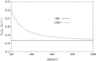
Figure 4: The $1/R$ dependence of the longitudinal polarization, $P_{L}(\hat{s},1/R)$ at $\hat{s}=0.5$.

Figure 5: The $1/R$ dependence of the normal polarization, $P_{N}(\hat{s},1/R)$ at $\hat{s}=0.5$.

Figure 6: The $1/R$ dependence of the transversal polarization, $P_{T}(\hat{s},1/R)$ at $\hat{s}=0.5$.

From these figures, we conclude that

• the UED predictions deviate considerably from those of the SM for all polarizations and both lepton channels at small values of compactification scale.

• The numerical values show that the $P_{L}$ and $P_{N}$ have measurable sizes for both leptons but $P_{T}$ is very small.

• In the case of $P_{L}$ and $|P_{N}|$, the UED predictions at lower values of $1/R$ are smaller than those of the SM at $\mu$ channel. However, for $\tau$ we have inverse situation. In the case of $P_{T}$, two lepton channels represent similar behavior.

3.5 Double Lepton Polarization Asymmetries

The present subsection encompasses our analysis on the double–lepton polarization asymmetries. In the case of both leptons polarizations, we define the following orthogonal unit vectors $s_{i}^{\pm\mu}$ with again $i=L,T$ or $N$ in the rest frame of double leptons (For details see for instance [25, 45, 46]):

$$s^{-\mu}_{L}\!\!\! = \!\!\!\left(0,\vec{e}_{L}^{\,-}\right)=\left(0,\frac{\vec{p}_{-}}{\left|\vec{p}_{-}\right|}\right)~{},$$

$$s^{-\mu}_{N}\!\!\! = \!\!\!\left(0,\vec{e}_{N}^{\,-}\right)=\left(0,\frac{\vec{p}_{\Sigma}\times\vec{p}_{-}}{\left|\vec{p}_{\Sigma}\times\vec{p}_{-}\right|}\right)~{},$$

$$s^{-\mu}_{T}\!\!\! = \!\!\!\left(0,\vec{e}_{T}^{\,-}\right)=\left(0,\vec{e}_{N}^{\,-}\times\vec{e}_{L}^{\,-}\right)~{},$$

$$s^{+\mu}_{L}\!\!\! = \!\!\!\left(0,\vec{e}_{L}^{\,+}\right)=\left(0,\frac{\vec{p}_{+}}{\left|\vec{p}_{+}\right|}\right)~{},$$

$$s^{+\mu}_{N}\!\!\! = \!\!\!\left(0,\vec{e}_{N}^{\,+}\right)=\left(0,\frac{\vec{p}_{\Sigma}\times\vec{p}_{+}}{\left|\vec{p}_{\Sigma}\times\vec{p}_{+}\right|}\right)~{},$$

$$s^{+\mu}_{T}\!\!\! = \!\!\!\left(0,\vec{e}_{T}^{\,+}\right)=\left(0,\vec{e}_{N}^{\,+}\times\vec{e}_{L}^{\,+}\right)~{},$$ (3.52)

where $\vec{p}_{\pm}$ and $\vec{p}_{\Sigma}$ are the three–momenta of the leptons $\ell^{\pm}$ and $\Sigma$ baryon. Now, by the help of the Lorentz boost, we transform these unit vectors from the rest frame of the leptons to center of mass (CM) frame of them along the longitudinal direction. As a result for the unit vectors $s_{L}^{\pm\mu}$ we get

$$\left(s^{\mp\mu}_{L}\right)_{CM}\!\!\! = \!\!\!\left(\frac{\left|\vec{p}_{\mp}\right|}{m_{\ell}}~{},\frac{E_{\ell}\vec{p}_{\mp}}{m_{\ell}\left|\vec{p}_{\mp}\right|}\right)~{},$$ (3.53)

where, $\vec{p}_{+}=-\vec{p}_{-}$; and $E_{\ell}$ and $m_{\ell}$ are the energy and mass of leptons in the CM frame, respectively. The remaining two unit vectors, $s_{N}^{\pm\mu}$, $s_{T}^{\pm\mu}$ do not change under the considered transformation. We now define the double–polarization asymmetries as:

$$P_{ij}(\hat{s},1/R)\!\!\! = \!\!\!\frac{\Big{(}\displaystyle\frac{d\Gamma(\vec{s}^{\,-}_{i},\vec{s}^{\,+}_{j})}{d\hat{s}}-\displaystyle\frac{d\Gamma(-\vec{s}^{\,-}_{i},\vec{s}^{\,+}_{j})}{d\hat{s}}\Big{)}-\Big{(}\displaystyle\frac{d\Gamma(\vec{s}^{\,-}_{i},-\vec{s}^{\,+}_{j})}{d\hat{s}}-\displaystyle\frac{d\Gamma(-\vec{s}^{\,-}_{i},-\vec{s}^{\,+}_{j})}{d\hat{s}}\Big{)}}{\Big{(}\displaystyle\frac{d\Gamma(\vec{s}^{\,-}_{i},\vec{s}^{\,+}_{j})}{d\hat{s}}+\displaystyle\frac{d\Gamma(-\vec{s}^{\,-}_{i},\vec{s}^{\,+}_{j})}{d\hat{s}}\Big{)}+\Big{(}\displaystyle\frac{d\Gamma(\vec{s}^{\,-}_{i},-\vec{s}^{\,+}_{j})}{d\hat{s}}+\displaystyle\frac{d\Gamma(-\vec{s}^{\,-}_{i},-\vec{s}^{\,+}_{j})}{d\hat{s}}\Big{)}}~{}.$$ (3.54)

Using this definition, we obtain the following $1/R$-dependent expressions for the double lepton polarization asymmetries :

$$P_{LN}(\hat{s},1/R)\!\!\! = \!\!\!\frac{16\pi m_{\Sigma_{b}}^{4}\hat{m}_{\ell}\sqrt{\lambda}}{\Delta(\hat{s},1/R)\sqrt{\hat{s}}}\mbox{\rm Im}\Bigg{\{}(1-r)(A_{1}^{\ast}D_{1}+B_{1}^{\ast}E_{1})+m_{\Sigma_{b}}\hat{s}(A_{1}^{\ast}E_{3}-A_{2}^{\ast}E_{1}+B_{1}^{\ast}D_{3}-B_{2}^{\ast}D_{1})$$ (3.55)

$$+ \!\!\!m_{\Sigma_{b}}\sqrt{r}\hat{s}(A_{1}^{\ast}D_{3}+A_{2}^{\ast}D_{1}+B_{1}^{\ast}E_{3}+B_{2}^{\ast}E_{1})-m_{\Sigma_{b}}^{2}\hat{s}^{2}\Big{(}B_{2}^{\ast}E_{3}+A_{2}^{\ast}D_{3}\Big{)}\Bigg{\}},$$

Figure 7: The $1/R$ dependence of the $P_{LN}(\hat{s},1/R)$ at $\hat{s}=0.5$.

$$P_{LT}(\hat{s},1/R)\!\!\! = \!\!\!\frac{16\pi m_{\Sigma_{b}}^{4}\hat{m}_{\ell}\sqrt{\lambda}v}{\Delta(\hat{s},1/R)\sqrt{\hat{s}}}\mbox{\rm Re}\Bigg{\{}(1-r)\Big{(}\left|D_{1}\right|^{2}+\left|E_{1}\right|^{2}\Big{)}-\hat{s}\Big{(}A_{1}D_{1}^{\ast}-B_{1}E_{1}^{\ast}\Big{)}$$ (3.56)

$$- \!\!\!m_{\Sigma_{b}}\hat{s}\Big{[}B_{1}D_{2}^{\ast}+(A_{2}+D_{2}-D_{3})E_{1}^{\ast}-A_{1}E_{2}^{\ast}-(B_{2}-E_{2}+E_{3})D_{1}^{\ast}\Big{]}$$

$$+ \!\!\!m_{\Sigma_{b}}\sqrt{r}\hat{s}\Big{[}A_{1}D_{2}^{\ast}+(A_{2}+D_{2}+D_{3})D_{1}^{\ast}-B_{1}E_{2}^{\ast}-(B_{2}-E_{2}-E_{3})E_{1}^{\ast}\Big{]}$$

$$+ \!\!\!m_{\Sigma_{b}}^{2}\hat{s}(1-r)(A_{2}D_{2}^{\ast}-B_{2}E_{2}^{\ast})-m_{\Sigma_{b}}^{2}\hat{s}^{2}(D_{2}D_{3}^{\ast}+E_{2}E_{3}^{\ast})\Bigg{\}},$$

$$P_{LL}(\hat{s},1/R)\!\!\! = \!\!\!\frac{16m_{\Sigma_{b}}^{4}}{3\Delta(\hat{s},1/R)}\mbox{\rm Re}\Bigg{\{}$$ (3.57)

$$- \!\!\!6m_{\Sigma_{b}}\sqrt{r}(1-r+\hat{s})\Big{[}\hat{s}(1+v^{2})(A_{1}A_{2}^{\ast}+B_{1}B_{2}^{\ast})-4\hat{m}_{\ell}^{2}(D_{1}D_{3}^{\ast}+E_{1}E_{3}^{\ast})\Big{]}$$

$$+ \!\!\!6m_{\Sigma_{b}}(1-r-\hat{s})\Big{[}\hat{s}(1+v^{2})(A_{1}B_{2}^{\ast}+A_{2}B_{1}^{\ast})+4\hat{m}_{\ell}^{2}(D_{1}E_{3}^{\ast}+D_{3}E_{1}^{\ast})\Big{]}$$

$$+ \!\!\!12\sqrt{r}\hat{s}(1+v^{2})\Big{(}A_{1}B_{1}^{\ast}+D_{1}E_{1}^{\ast}+m_{\Sigma_{b}}^{2}\hat{s}A_{2}B_{2}^{\ast}\Big{)}$$

$$+ \!\!\!12m_{\Sigma_{b}}^{2}\hat{m}_{\ell}^{2}\hat{s}(1+r-\hat{s})\left(\left|D_{3}\right|^{2}+\left|E_{3}^{\ast}\right|^{2}\right)$$

$$- \!\!\!(1+v^{2})\Big{[}1+r^{2}-r(2-\hat{s})+\hat{s}(1-2\hat{s})\Big{]}\Big{(}\left|A_{1}\right|^{2}+\left|B_{1}\right|^{2}\Big{)}$$

$$- \!\!\!\Big{[}(5v^{2}-3)(1-r)^{2}+4\hat{m}_{\ell}^{2}(1+r)+2\hat{s}(1+8\hat{m}_{\ell}^{2}+r)-4\hat{s}^{2}\Big{]}\Big{(}\left|D_{1}\right|^{2}+\left|E_{1}\right|^{2}\Big{)}$$

$$- \!\!\!m_{\Sigma_{b}}^{2}(1+v^{2})\hat{s}\Big{[}2+2r^{2}-\hat{s}(1+\hat{s})-r(4+\hat{s})\Big{]}\big{(}\left|A_{2}\right|^{2}+\left|B_{2}\right|^{2}\Big{)}$$

$$- \!\!\!2m_{\Sigma_{b}}^{2}\hat{s}v^{2}\Big{[}2(1+r^{2})-\hat{s}(1+\hat{s})-r(4+\hat{s})\Big{]}\Big{(}\left|D_{2}\right|^{2}+\left|E_{2}\right|^{2}\Big{)}$$

$$+ \!\!\!12m_{\Sigma_{b}}\hat{s}(1-r-\hat{s})v^{2}\Big{(}D_{1}E_{2}^{\ast}+D_{2}E_{1}^{\ast}\Big{)}$$

$$- \!\!\!12m_{\Sigma_{b}}\sqrt{r}\hat{s}(1-r+\hat{s})v^{2}\Big{(}D_{1}D_{2}^{\ast}+E_{1}E_{2}^{\ast}\Big{)}$$

$$+ \!\!\!24m_{\Sigma_{b}}^{2}\sqrt{r}\hat{s}\Big{(}\hat{s}v^{2}D_{2}E_{2}^{\ast}+2\hat{m}_{\ell}^{2}D_{3}E_{3}^{\ast}\Big{)}\Bigg{\}},$$

$$P_{NL}(\hat{s},1/R)\!\!\! = \!\!\!-\frac{16\pi m_{\Sigma_{b}}^{4}\hat{m}_{\ell}\sqrt{\lambda}}{\Delta(\hat{s},1/R)\sqrt{\hat{s}}}\mbox{\rm Im}\Bigg{\{}(1-\hat{r}_{\Sigma})(A_{1}^{\ast}D_{1}+B_{1}^{\ast}E_{1})+m_{\Sigma_{b}}\hat{s}(A_{1}^{\ast}E_{3}-A_{2}^{\ast}E_{1}+B_{1}^{\ast}D_{3}-B_{2}^{\ast}D_{1})$$ (3.58)

$$- \!\!\!m_{\Sigma_{b}}\sqrt{\hat{r}_{\Sigma}}\hat{s}(A_{1}^{\ast}D_{3}+A_{2}^{\ast}D_{1}+B_{1}^{\ast}E_{3}+B_{2}^{\ast}E_{1})-m_{\Sigma_{b}}^{2}\hat{s}^{2}\Big{(}B_{2}^{\ast}E_{3}+A_{2}^{\ast}D_{3}\Big{)}\Bigg{\}},$$

Figure 8: The $1/R$ dependence of the $P_{LT}(\hat{s},1/R)$ at $\hat{s}=0.5$.

Figure 9: The $1/R$ dependence of the $P_{NL}(\hat{s},1/R)$ at $\hat{s}=0.5$.

$$P_{NN}(\hat{s},1/R)\!\!\! = \!\!\!\frac{32m_{\Sigma_{b}}^{4}}{3\hat{s}\Delta(\hat{s},1/R)}\mbox{\rm Re}\Bigg{\{}24\hat{m}_{\ell}^{2}\sqrt{r}\hat{s}(A_{1}B_{1}^{\ast}+D_{1}E_{1}^{\ast})$$ (3.59)

$$- \!\!\!12m_{\Sigma_{b}}\hat{m}_{\ell}^{2}\sqrt{r}\hat{s}(1-r+\hat{s})(A_{1}A_{2}^{\ast}+B_{1}B_{2}^{\ast})$$

$$+ \!\!\!6m_{\Sigma_{b}}\hat{m}_{\ell}^{2}\hat{s}\Big{[}m_{\Sigma_{b}}\hat{s}(1+r-\hat{s})\Big{(}\left|D_{3}\right|^{2}+\left|E_{3}\right|^{2}\Big{)}+2\sqrt{r}(1-r+\hat{s})(D_{1}D_{3}^{\ast}+E_{1}E_{3}^{\ast})\Big{]}$$

$$+ \!\!\!12m_{\Sigma_{b}}\hat{m}_{\ell}^{2}\hat{s}(1-r-\hat{s})(A_{1}B_{2}^{\ast}+A_{2}B_{1}^{\ast}+D_{1}E_{3}^{\ast}+D_{3}E_{1}^{\ast})$$

$$- \!\!\![\lambda\hat{s}+2\hat{m}_{\ell}^{2}(1+r^{2}-2r+r\hat{s}+\hat{s}-2\hat{s}^{2})]\Big{(}\left|A_{1}\right|^{2}+\left|B_{1}\right|^{2}-\left|D_{1}\right|^{2}-\left|E_{1}\right|^{2}\Big{)}$$

$$+ \!\!\!24m_{\Sigma_{b}}^{2}\hat{m}_{\ell}^{2}\sqrt{r}\hat{s}^{2}(A_{2}B_{2}^{\ast}+D_{3}E_{3}^{\ast})-m_{\Sigma_{b}}^{2}\lambda\hat{s}^{2}v^{2}\Big{(}\left|D_{2}\right|^{2}+\left|E_{2}\right|^{2}\Big{)}$$

$$+ \!\!\!m_{\Sigma_{b}}^{2}\hat{s}\{\lambda\hat{s}-2\hat{m}_{\ell}^{2}[2(1+r^{2})-\hat{s}(1+\hat{s})-r(4+\hat{s})]\}\Big{(}\left|A_{2}\right|^{2}+\left|B_{2}\right|^{2}\Big{)}\Bigg{\}},$$

Figure 10: The $1/R$ dependence of the $P_{NN}(\hat{s},1/R)$ at $\hat{s}=0.5$.

$$P_{NT}(\hat{s},1/R)\!\!\! = \!\!\!\frac{64m_{\Sigma_{b}}^{4}\lambda v}{3\Delta(\hat{s},1/R)}\mbox{\rm Im}\Bigg{\{}(A_{1}D_{1}^{\ast}+B_{1}E_{1}^{\ast})+m_{\Sigma_{b}}^{2}\hat{s}(A_{2}^{\ast}D_{2}+B_{2}^{\ast}E_{2})\Bigg{\}},$$ (3.60)

Figure 11: The $1/R$ dependence of the $P_{NT}(\hat{s},1/R)$ at $\hat{s}=0.5$.

$$P_{TL}(\hat{s},1/R)\!\!\! = \!\!\!\frac{16\pi m_{\Sigma_{b}}^{4}\hat{m}_{\ell}\sqrt{\lambda}v}{\Delta(\hat{s},1/R)\sqrt{\hat{s}}}\mbox{\rm Re}\Bigg{\{}(1-\hat{r}_{\Sigma})\Big{(}\left|D_{1}\right|^{2}+\left|E_{1}\right|^{2}\Big{)}+\hat{s}\Big{(}A_{1}D_{1}^{\ast}-B_{1}E_{1}^{\ast}\Big{)}$$ (3.61)

$$+ \!\!\!m_{\Sigma_{b}}\hat{s}\Big{[}B_{1}D_{2}^{\ast}+(A_{2}-D_{2}+D_{3})E_{1}^{\ast}-A_{1}E_{2}^{\ast}-(B_{2}+E_{2}-E_{3})D_{1}^{\ast}\Big{]}$$

$$- \!\!\!m_{\Sigma_{b}}\sqrt{\hat{r}_{\Sigma}}\hat{s}\Big{[}A_{1}D_{2}^{\ast}+(A_{2}-D_{2}-D_{3})D_{1}^{\ast}-B_{1}E_{2}^{\ast}-(B_{2}+E_{2}+E_{3})E_{1}^{\ast}\Big{]}$$

$$- \!\!\!m_{\Sigma_{b}}^{2}\hat{s}(1-\hat{r}_{\Sigma})(A_{2}D_{2}^{\ast}-B_{2}E_{2}^{\ast})-m_{\Sigma_{b}}^{2}\hat{s}^{2}(D_{2}D_{3}^{\ast}+E_{2}E_{3}^{\ast})\Bigg{\}},$$

Figure 12: The $1/R$ dependence of the $P_{TL}(\hat{s},1/R)$ at $\hat{s}=0.5$.

$$P_{TN}(\hat{s},1/R)\!\!\! = \!\!\!-\frac{64m_{\Sigma_{b}}^{4}\lambda v}{3\Delta(\hat{s},1/R)}\mbox{\rm Im}\Bigg{\{}(A_{1}D_{1}^{\ast}+B_{1}E_{1}^{\ast})+m_{\Sigma_{b}}^{2}\hat{s}(A_{2}^{\ast}D_{2}+B_{2}^{\ast}E_{2})\Bigg{\}},$$ (3.62)

Figure 13: The $1/R$ dependence of the $P_{TN}(\hat{s},1/R)$ at $\hat{s}=0.5$.

$$P_{TT}(\hat{s},1/R)\!\!\! = \!\!\!\frac{32m_{\Sigma_{b}}^{4}}{3\hat{s}\Delta(\hat{s},1/R)}\mbox{\rm Re}\Bigg{\{}-24\hat{m}_{\ell}^{2}\sqrt{r}\hat{s}(A_{1}B_{1}^{\ast}+D_{1}E_{1}^{\ast})$$ (3.63)

$$- \!\!\!12m_{\Sigma_{b}}\hat{m}_{\ell}^{2}\sqrt{r}\hat{s}(1-r+\hat{s})(D_{1}D_{3}^{\ast}+E_{1}E_{3}^{\ast})-24m_{\Sigma_{b}}^{2}\hat{m}_{\ell}^{2}\sqrt{r}\hat{s}^{2}(A_{2}B_{2}^{\ast}+D_{3}E_{3}^{\ast})$$

$$- \!\!\!6m_{\Sigma_{b}}\hat{m}_{\ell}^{2}\hat{s}\Big{[}m_{\Sigma_{b}}\hat{s}(1+r-\hat{s})\Big{(}\left|D_{3}\right|^{2}+\left|E_{3}\right|^{2}\Big{)}-2\sqrt{r}(1-r+\hat{s})(A_{1}A_{2}^{\ast}+B_{1}B_{2}^{\ast})\Big{]}$$

$$- \!\!\!12m_{\Sigma_{b}}\hat{m}_{\ell}^{2}\hat{s}(1-r-\hat{s})(A_{1}B_{2}^{\ast}+A_{2}B_{1}^{\ast}+D_{1}E_{3}^{\ast}+D_{3}E_{1}^{\ast})$$

$$- \!\!\![\lambda\hat{s}-2\hat{m}_{\ell}^{2}(1+r^{2}-2r+r\hat{s}+\hat{s}-2\hat{s}^{2})]\Big{(}\left|A_{1}\right|^{2}+\left|B_{1}\right|^{2}\Big{)}$$

$$+ \!\!\!m_{\Sigma_{b}}^{2}\hat{s}\{\lambda\hat{s}+\hat{m}_{\ell}^{2}[4(1-r)^{2}-2\hat{s}(1+r)-2\hat{s}^{2}]\}\Big{(}\left|A_{2}\right|^{2}+\left|B_{2}\right|^{2}\Big{)}$$

$$+ \!\!\!\{\lambda\hat{s}-2\hat{m}_{\ell}^{2}[5(1-r)^{2}-7\hat{s}(1+r)+2\hat{s}^{2}]\}\Big{(}\left|D_{1}\right|^{2}+\left|E_{1}\right|^{2}\Big{)}$$

$$- \!\!\!m_{\Sigma_{b}}^{2}\lambda\hat{s}^{2}v^{2}\Big{(}\left|D_{2}\right|^{2}+\left|E_{2}\right|^{2}\Big{)}\Bigg{\}},$$

Figure 14: The $1/R$ dependence of the $P_{TT}(\hat{s},1/R)$ at $\hat{s}=0.5$.

where, $\hat{m}_{l}=\frac{m_{l}}{m_{\Sigma_{b}}}$. The dependence of various double lepton polarization asymmetries are presented in Figures 7-14. Our numerical analysis show that

• there are also considerable discrepancies between two model predictions at lower values of the compactification scale.

• The $P_{LL}$, $P_{NN}$, $P_{TT}$ and $P_{LT}$ are very sensitive to new physics effects, while the effects of UED on $P_{TN}$, $P_{TL}$, $P_{NT}$, $P_{NL}$ and $P_{LN}$ are small.

• Except than the $P_{TT}$, all polarizations have the same sign for both leptons.

3.6 Physical Observables Considering Uncertainties of the Form Factors

In the previous subsections, we numerically analyzed the physical quantities under consideration and discussed their dependencies on the compactification factor of extra dimension when only the central values of the form factors are considered. Here, we discuss how the uncertainties of the form factors as the main inputs affect the obtained results. For this aim, we present dependencies of different physical observables for $\Sigma_{b}\rightarrow\Sigma\ell^{+}\ell^{-}$ on $1/R$ when the errors of the form factors are taken into account in figures 15-27.

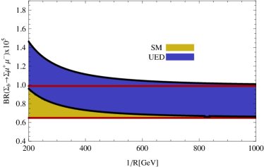
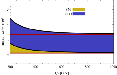
Figure 15: The $1/R$ dependence of the branching ratio for $\Sigma_{b}\rightarrow\Sigma\ell^{+}\ell^{-}$ at $\hat{s}=0.5$ when errors of the form factors are taken into account. The Brown-Yellow bands surrounded by red lines refer to the SM, while the blue bands surrounded by black lines denote the UED results.

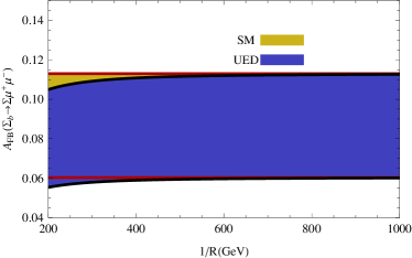
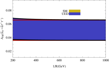
Figure 16: The same as figure 15 but for forward-backward asymmetry.

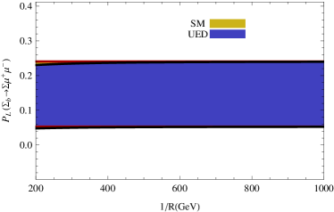
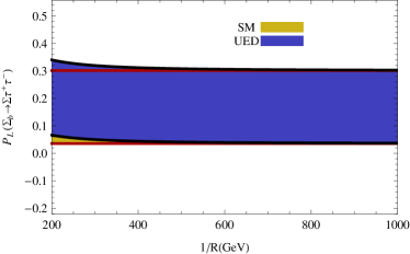
Figure 17: The same as figure 15 but for $P_{L}$.

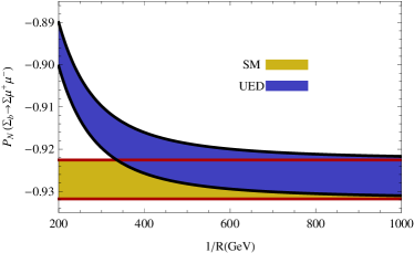
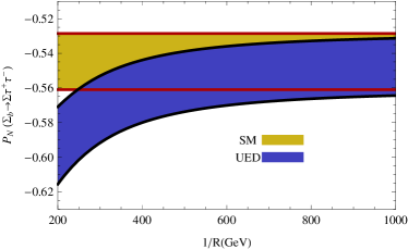
Figure 18: The same as figure 15 but for $P_{N}$.

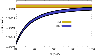
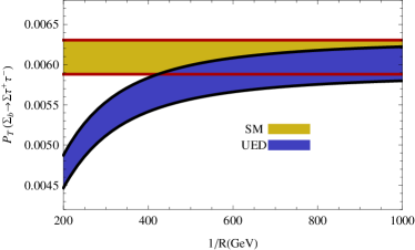
Figure 19: The same as figure 15 but for $P_{T}$.

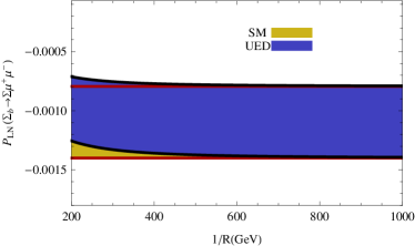
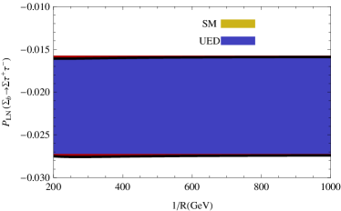
Figure 20: The same as figure 15 but for $P_{LN}$.

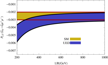
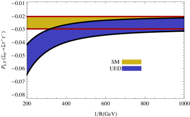
Figure 21: The same as figure 15 but for $P_{LT}$.

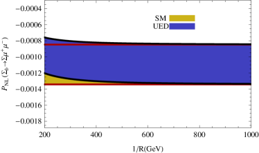
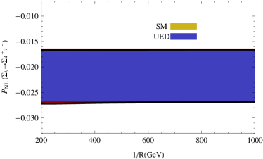
Figure 22: The same as figure 15 but for $P_{NL}$.

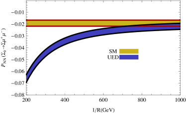
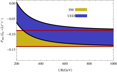
Figure 23: The same as figure 15 but for $P_{NN}$.

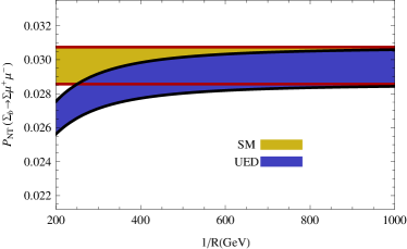
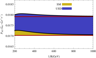
Figure 24: The same as figure 15 but for $P_{NT}$.

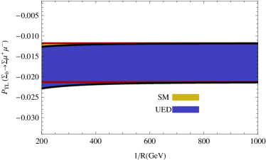
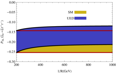
Figure 25: The same as figure 15 but for $P_{TL}$.

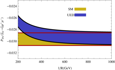
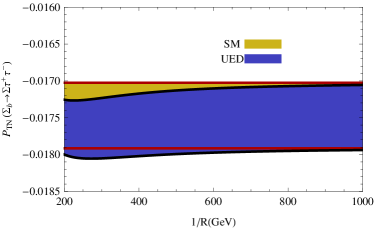
Figure 26: The same as figure 15 but for $P_{TN}$.

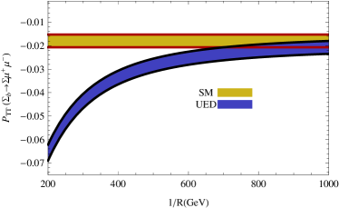
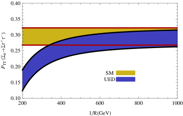
Figure 27: The same as figure 15 but for $P_{TT}$.

From these figures we see that in all cases, the SM and UED bands intersect each other in some regions. In some cases like $P_{N}$ at $\mu$ channel as well as $P_{T}$, $P_{TT}$, $P_{NN}$ and $P_{LT}$ at both lepton channels, the errors of the form factors can not kill the differences between the UED and SM predictions at small values of the compactification factor. In the case of forward-backward asymmetry and longitudinal baryon polarization for both leptons; $P_{LN}$ and $P_{NL}$ at $\tau$ channel as well as $P_{TL}$ at $\mu$ channel, the differences between two model predictions are killed by the uncertainties of the form factors. For the other cases like branching ratio at both lepton channels; $P_{LN}$ and $P_{NL}$ at $\mu$ channel; and $P_{NT}$, $P_{TN}$ and $P_{TL}$ at $\tau$ channel, we have intermediate situation and see some small but considerable regions out of the intersection parts of the SM and UED predictions.

4 Conclusion

In the present study, we found a lower limit for the compactification scale of extra dimension comparing the recent experimental data on the branching ratio of baryonic FCNC $\Lambda_{b}\rightarrow\Lambda\mu^{+}\mu^{-}$ transition and our previous theoretical work. We put an approximately $250~{}GeV$ for lower limit of the compactification factor in the presence of a single UED. This limit is in a good consistency with the lower limit very recently obtained via comparison between the experimental data and theoretical results (containing a single UED) on the branching fraction of the mesonic $B\rightarrow K\eta\gamma$ [34] channel. Our result is also comparable with some other limits previously obtained in other mesonic channels as well as some electroweak precision tests [29, 4, 5]. However, our lower limit on $1/R$ is small compared to the one also obtained in $B\rightarrow K\eta\gamma$ channel but in the presence of 2 UEDs as well as obtained from some other mesonic decay channels, electroweak precision tests, some cosmological constraints and ATLAS results discussed in section 2 [30, 31, 32, 33]. To improve our limit, we need the expressions of the Wilson coefficients $C_{9}^{eff}$ and $C_{10}$ calculated in the presence of 2 UEDs, theoretically. From the experimental point of view, we are waiting for the results of LHCb on the physical observables related to the $\Lambda_{b}\rightarrow\Lambda\mu^{+}\mu^{-}$ channel to confirm the CDF data [1].

In the second part, we have analyzed the other baryonic $\Sigma_{b}\rightarrow\Sigma\ell^{+}\ell^{-}$ decay channel also in UED scenario. Using the form factors recently available and calculated via light cone QCD sum rules in full theory, we have discussed sensitivity of many related physical observables such as branching ratio, forward-backward asymmetry, baryon polarizations and double lepton polarization asymmetries on the compactification factor of extra dimension. We have observed over all sizable discrepancies between the UED and SM predictions at lower values of the compactification scale when we considered the central values of the form factors as the main inputs. Although these discrepancies are killed by uncertainties of the form factors for some cases discussed in the body text, for many observables we have still considerable differences between two model predictions. These can be considered as indications for existing the KK modes and extra dimensions should we search for them at hadron colliders. The order of branching fraction in $\Sigma_{b}\rightarrow\Sigma\ell^{+}\ell^{-}$ decay channel indicates that this channel is accessible at LHC.

5 Acknowledgement

We thank V. N. Şenoğuz for useful discussions on lower limit of compactification scale.

References

- [1] T. Aaltonen et al. [ CDF Collaboration ], “Observation of the Baryonic Flavor-Changing Neutral Current Decay ”, Phys. Rev. Lett. 107, 201802 (2011), arXiv:1107.3753 [hep-ex].
- [2] Our personal communications with Yasmine Sara Amhis from LHCb Collaboration.
- [3] K. Azizi, N. Katırcı, “Investigation of the transition in universal extra dimension using form factors from full QCD”, JHEP 1101 (2011) 087, arXiv:1011.5647 [hep-ph].
- [4] T. Appelquist, H. C. Cheng and B. A. Dobrescu, “Bounds on universal extra dimensions”, Phys. Rev. D 64, 035002 (2001), arXiv:hep-ph/0012100.
- [5] T. Appelquist, H. U. Yee, “Universal extra dimensions and the Higgs boson mass”, Phys. Rev. D 67, 055002 (2003), arXiv:hep-ph/0211023.
- [6] I. Antoniadis, “A possible new dimension at a few TeV”, Phys. Lett. B 246, 377 (1990).
- [7] I. Antoniadis, N. Arkani-Hamed, S. Dimopoulos and G. Dvali, “New dimensions at a millimeter to a fermi and superstrings at a TeV”, Phys. Lett. B 436, 257 (1998), arXiv:hep-ph/9804398.
- [8] N. Arkani-Hamed, S. Dimopoulos and G. Dvali, “The hierarchy problem and new dimensions at a millimeter”, Phys. Lett. B 429, 263 (1998), arXiv:hep-ph/9803315.
- [9] N. Arkani-Hamed, S. Dimopoulos and G. Dvali, “Phenomenology, astrophysics, and cosmology of theories with submillimeter dimensions and TeV scale quantum gravity”, Phys. Rev. D 59, 086004 (1999), arXiv:hep-ph/9807344.
- [10] L. Randall, R. Sundrum, “An Alternative to Compactification”, Phys. Rev. Lett. 83, 4690 (1999), arXiv:hep-th/9906064.
- [11] L. Randall, R. Sundrum, “Large Mass Hierarchy from a Small Extra Dimension”, Phys. Rev. Lett. 83, 3370 (1999), arXiv:hep-ph/9905221.
- [12] T. M. Aliev, K. Azizi, M. Savci, “Analysis of the decay in QCD”, Phys. Rev. D 81, 056006 (2010), arXiv:1001.0227 [hep-ph].
- [13] K. Azizi, M. Bayar, A. Ozpineci, Y. Sarac, H. Sundu, “Semileptonic transition of to in Light Cone QCD Sum Rules”, Phys. Rev. D 85, 016002 (2012), arXiv:1112.5147 [hep-ph].
- [14] A. J. Buras, M. Spranger and A. Weiler, “The impact of universal extra dimensions on the unitarity triangle and rare K and B decays”, Nucl. Phys. B 660, 225 (2003), arXiv:hep-ph/0212143.
- [15] A. J. Buras, A. Poschenrieder, M. Spranger, A. Weiler “The Impact of Universal Extra Dimensions on , , , , and ”, Nucl. Phys. B 678, 455 (2004), arXiv:hep-ph/0306158.
- [16] P. Colangelo, F. De Fazio, R. Ferrandes, T. N. Pham, “Exclusive , and transitions in a scenario with a single Universal Extra Dimension”, Phys. Rev. D 73, 115006 (2006), arXiv:hep-ph/0604029.
- [17] V. Bashiry, K. Azizi, “Systematic analysis of the in the universal extra dimension”, JHEP 1202 (2012) 021, arXiv:1112.5243 [hep-ph].
- [18] N. Katirci, K. Azizi, “B to strange tensor meson transition in a model with one universal extra dimension”, JHEP 1107 (2011) 043, arXiv:1105.3636 [hep-ph].
- [19] V. Bashiry, M. Bayar, K. Azizi, “Double-lepton polarization asymmetries and polarized forward backward asymmetries in the rare decays in a single universal extra dimension scenario”, Phys. Rev. D 78, 035010 (2008), arXiv:0808.1807 [hep-ph].
- [20] Yu-Ming Wang, M. Jamil Aslam, Cai-Dian Lu, “Rare decays of and in universal extra dimension model”, Eur. Phys. J. C 59, 847 (2009), arXiv:0810.0609 [hep-ph].
- [21] T. M. Aliev, M. Savcı, “ decay in universal extra dimensions”, Eur. Phys. J. C 50, 91 (2007), arXiv:hep-ph/0606225.
- [22] F. De Fazio, “Rare B decays in a single Universal Extra Dimension scenario”, Nucl. Phys. Proc. Suppl. 174, 185 (2007), arXiv:hep-ph/0610208.
- [23] B. B. Sirvanli, K. Azizi, Y. Ipekoglu, “Double-lepton polarization asymmetries and branching ratio in transition from universal extra dimension model”, JHEP 1101 (2011) 069, arXiv:1011.1469 [hep-ph].
- [24] K. Azizi, N. K. Pak, B. B. Sirvanli, “Double-Lepton Polarization Asymmetries and Branching Ratio of the transition in Universal Extra Dimension”, JHEP 1202 (2012) 034, arXiv:1112.2927 [hep-ph].
- [25] T. M. Aliev, M. Savci, B. B. Sirvanli, “Double-lepton polarization asymmetries in decay in universal extra dimension model”, Eur. Phys. J. C 52, 375 (2007), arXiv:hep-ph/0608143.
- [26] I. Ahmed, M. A. Paracha, M. J. Aslam, “Exclusive decay in model with single universal extra dimension”, Eur. Phys. J. C 54, 591 (2008), arXiv:0802.0740 [hep-ph].
- [27] P. Colangelo, F. De Fazio, R. Ferrandes, T. N. Pham, “Spin effects in rare and decays in a single universal extra dimension scenario”, Phys. Rev. D 74, 115006 (2006), arXiv:hep-ph/0610044.
- [28] R. Mohanta and A. K. Giri, “Study of FCNC-mediated rare decays in a single universal extra dimension scenario”, Phys. Rev. D 75, 035008 (2007), arXiv:hep-ph/0611068.
- [29] K. Agashe, N. G. Deshpande, G. H. Wu, “Universal extra dimensions and ”, Phys. Lett. B 514, 309 (2001), arXiv:hep-ph/0105084; “Can extra dimensions accessible to the SM explain the recent measurement of anomalous magnetic moment of the muon?”,B 511, 85 (2001), arXiv:hep-ph/0103235; T. Appelquist, B. A. Dobrescu, “Universal Extra Dimensions and the Muon Magnetic Moment”, Phys. Lett. B 516, 8 (2001), arXiv:hep-ph/0106140.
- [30] I. Gogoladze and C. Macesanu, “Precision electroweak constraints on universal extra dimensions revisited”, Phys. Rev. D 74, 093012 (2006), arXiv:hep-ph/0605207.
- [31] J. A. R. Cembranos, J. L. Feng and L. E. Strigari, “Exotic collider signals from the complete phase diagram of minimal universal extra dimensions”, Phys. Rev. D 75, 036004 (2007), arXiv:hep-ph/0612157.
- [32] U. Haisch and A. Weiler, “Bound on minimal universal extra dimensions from ”, Phys. Rev. D 76, 034014 (2007), arXiv:hep-ph/0703064.
- [33] ATLAS Collaboration, “Search for supersymmetry with jets and missing transverse momentum: Additional model interpretations”, ATLAS-CONF-2011-155, November 13 (2011).
- [34] P. Biancofiore, P. Colangelo, F. Fazio, “ decays in the standard model and in two scenarios with universal extra dimensions”, arXiv:1202.2289 [hep-ph].
- [35] M. V. Carlucci, P. Colangelo and F. De Fazio, “Rare decays to and final states”, Phys. Rev. D 80, 055023 (2009), arXiv:0907.2160 [hep-ph]; P. Colangelo, F. De Fazio, R. Ferrandes and T. N. Pham, “Exclusive , and transitions in a scenario with a single Universal Extra Dimension”, Phys. Rev. D 73, 115006 (2006), arXiv:hep-ph/0604029; P. Colangelo, F. De Fazio, R. Ferrandes and T. N. Pham, “FCNC and transitions: Standard model versus a single universal extra dimension scenario”, Phys. Rev. D 77, 055019 (2008), arXiv:0709.2817 [hep-ph].
- [36] M. Misiak, “The and decays with next-to-leading logarithmic QCD-corrections”, Nucl. Phys. B 393, 23 (1993); Erratum-ibid B 439, 161 (1995).
- [37] B. Buras, M. Munz, “Effective Hamiltonian for Beyond Leading Logarithms in the NDR and HV Schemes”, Phys. Rev. D 52, 186 (1995), arXiv:hep-ph/9501281.
- [38] A. Buras, M. Misiak, M. Münz and S. Pokorski, “Theoretical Uncertainties and Phenomenological Aspects of Decay”, Nucl. Phys. B 424, 374 (1994), arXiv:hep-ph/9311345.
- [39] T. M. Aliev, A. Ozpineci, M. Savci, “Exclusive decay beyond standard model”, Nucl. Phys. B 649, 168 (2003).
- [40] A. K. Giri, R. Mohanta, “Study of FCNC mediated Z boson effect in the semileptonic rare baryonic decays ”, Eur. Phys. J. C 45, 151 (2006), arXiv:hep-ph/0510171.
- [41] K. Nakamura et al. (Particle Data Group), J. Phys. G 37, 075021 (2010).
- [42] T. M. Aliev, A. Ozpineci, M. Savci, C. Yuce, “T violation in decay beyond standard model”, Phys. Lett. B 542, 229 (2002), arXiv:hep-ph/0206014.
- [43] T. M. Aliev, A. Ozpineci, M. Savci, “Model independent analysis of baryon polarizations in decay”, Phys. Rev. D 67, 035007 (2003), arXiv:hep-ph/0211447.
- [44] T. M. Aliev, A. Ozpineci, M. Savci, “Explicit expressions of the baryon polarizations in decay for the massive lepton case”, arXiv:hep-ph/0301019.
- [45] T. M. Aliev, V. Bashiry, M. Savci, “Double-lepton polarization asymmetries in decay”, Eur. Phys. J. C 38, 283 (2004), arXiv:hep-ph/0409275.
- [46] W. Bensalem, D. London, N. Sinha and R. Sinha, “Lepton Polarization and Forward-Backward Asymmetries in ”, Phys. Rev. D 67, 034007 (2003), arXiv:hep-ph/0209228.