Harmonic knots

Abstract

The harmonic knot ${\rm H}(a,b,c)$ is parametrized as $K(t)=(T_{a}(t),T_{b}(t),T_{c}(t))$ where $a$, $b$ and $c$ are pairwise coprime integers and $T_{n}$ is the degree $n$ Chebyshev polynomial of the first kind. We classify the harmonic knots ${\rm H}(a,b,c)$ for $a\leq 4.$ We study the knots ${\rm H}(2n-1,2n,2n+1),$ the knots ${\rm H}(5,n,n+1),$ and give a table of the simplest harmonic knots.

keywords: Long knots, polynomial curves, Chebyshev curves, rational knots, continued fractions
Mathematics Subject Classification 2000: 14H50, 57M25, 11A55, 14P99

1 Introduction

A harmonic curve (or Chebyshev curve) is defined to be a curve which admits a parametrization $x=T_{a}(t),\,y=T_{b}(t),\,z=T_{c}(t)$ where $t\in{\bf R},$ $a$, $b$ and $c$ are integers, and $T_{n}(t)$ are the Chebyshev polynomials defined by $T_{n}(\cos t)=\cos nt.$ A harmonic knot is a nonsingular harmonic curve, it is a long knot. In 1897 Comstock proved that a harmonic curve is a knot if and only if $a,b,c$ are pairwise coprime integers ([Com, KP2, Fr]).

We observed in [KP1] that the trefoil can be parametrized by Chebyshev polynomials: $x=T_{3}(t),\,y=T_{4}(t),\,z=T_{5}(t)$. This led us to study harmonic knots in [KP2].

Harmonic knots are polynomial analogues of the famous Lissajous knots ([BDHZ, BHJS, Cr, HZ, JP, La1, La2]). However, they are very different: there are only two known examples of knots which are both Lissajous and harmonic, the knots $5_{2}$ and $7_{5}.$

We proved in [KP2] that the harmonic knot ${\rm H}(a,b,ab-a-b)$ is alternating, and deduced that there are infinitely many amphicheiral harmonic knots and infinitely many strongly invertible harmonic knots. We also proved that the torus knot $T(2,2n+1)$ is the harmonic knot ${\rm H}(3,3n+2,3n+1)$.

The harmonic knots ${\rm H}(3,b,c)$ are classified in [KP3]; they are two-bridge knots and their Schubert fractions ${\displaystyle{{\alpha}\overwithdelims. .{\beta}}}$ satisfy $\beta^{2}\equiv\pm 1\,(\hbox{\rm mod}\,\alpha)$.

In this article, we give the classification of the harmonic knots ${\rm H}(4,b,c)$ for $b$ and $c$ coprime odd integers. We also study some infinite families of harmonic knots for $a\geq 5.$

In section 2 we recall the Conway notation for two-bridge knots, and the computation of their Schubert fractions. The knots ${\rm H}(4,b,c)$ are two-bridge knots, and their Schubert fractions are given by continued fractions of the form $[\pm 1,\pm 2,\ldots,\pm 1,\pm 2].$ In section 3 we compute the Schubert fractions of the knots ${\rm H}(4,b,c),$ and we deduce their classification.

Theorem 3.6. Let $b$ and $c$ be relatively prime odd integers, and let $K={\rm H}(4,b,c).$ There is a unique pair $(b^{\prime},c^{\prime})$ such that (up to mirroring)

$$K={\rm H}(4,b^{\prime},c^{\prime}),\ b^{\prime}<c^{\prime}<3b^{\prime},\ b^{\prime}\not\equiv c^{\prime}\,(\hbox{\rm mod}\,4).$$

$K$ has a Schubert fraction ${\displaystyle{{\alpha}\overwithdelims. .{\beta}}}$ such that $\beta^{2}\equiv\pm 2\,(\hbox{\rm mod}\,\alpha).$ Furthermore, there is an algorithm to find $(b^{\prime},c^{\prime}),$ and the crossing number of $K$ is $N=(3b^{\prime}+c^{\prime}-2)/4.$

We notice that the trefoil is the only knot which is both of form ${\rm H}(3,b,c)$ and ${\rm H}(4,b,c).$ In section 4 we study some families of harmonic knots ${\rm H}(a,b,c)$ with $a\geq 5.$ In general their bridge number is greater than two, this is why the following result is surprising.

Theorem 4.4. The harmonic knot ${\rm H}(2n-1,2n,2n+1)$ is isotopic to the two-bridge harmonic knot ${\rm H}(4,2n-1,2n+1),$ up to mirror symmetry.

We also find an infinite family of two-bridge harmonic knots which are not of the form ${\rm H}(a,b,c)$ for $a\leq 4$:

Theorem 4.5.
The knot ${\rm H}(5,5n+1,5n+2)$ is the two-bridge knot of Conway form $C(2n+1,2n).$
The knot ${\rm H}(5,5n+3,5n+4)$ is the two-bridge knot of Conway form $C(2n+1,2n+2).$
Except for ${\rm H}(5,6,7)={\rm H}(4,5,7)$ and ${\rm H}(5,3,4),$ these knots are not of the form ${\rm H}(a,b,c)$ with $a\leq 4.$

Then, we identify the knots ${\rm H}(a,b,c)$ for $(a-1)(b-1)\leq 30.$ Our examples show that harmonic knots are not necessarily prime, nor reversible.

2 Continued fractions and two-bridge knots

A two-bridge knot (or link) admits a diagram in Conway form. This form, denoted by $C(a_{1},a_{2},\ldots,a_{n})$ where $a_{i}\in{\bf Z}$, is explained by the following picture (see [Con], [Mu, p. 187]).

\psfrag{a}{\small$a_{1}$}\psfrag{b}{\small$a_{2}$}\psfrag{c}{\small$a_{n-1}$}\psfrag{d}{\small$a_{n}$}\includegraphics{kr2bbf.eps}

\psfrag{a}{\small$a_{1}$}\psfrag{b}{\small$a_{2}$}\psfrag{c}{\small$a_{n-1}$}\psfrag{d}{\small$a_{n}$}\includegraphics{kr1bbf.eps}

Figure 1: Conway forms for polynomial knots ($n$ odd, and $n$ even)

The number of twists is denoted by the integer $\left|a_{i}\right|$, and the sign of $a_{i}$ , called the Kauffman sign, is defined as follows: if $i$ is odd, then the right twist is positive, if $i$ is even, then the right twist is negative. In Figure 1 the $a_{i}$ are positive (the $a_{1}$ first twists are right twists).

The two-bridge knots (or links) are classified by their Schubert fractions

$${\displaystyle{{\alpha}\overwithdelims. .{\beta}}}=a_{1}+{\displaystyle{{1}\overwithdelims. .{a_{2}+{\displaystyle{{1}\overwithdelims. .{\cdots+{\displaystyle{{1}\overwithdelims. .{a_{n}}}}}}}}}}=[a_{1},\ldots,a_{n}],\quad\alpha>0,\ \ a_{i}\in{\bf Z}\cup\{\infty\}.$$

A two-bridge knot (or link) with Schubert fraction ${\displaystyle{{\alpha}\overwithdelims. .{\beta}}}$ is denoted by $S\bigl{(}{\displaystyle{{\alpha}\overwithdelims. .{\beta}}}\bigr{)}.$ The two-bridge knots (or links) $S({\displaystyle{{\alpha}\overwithdelims. .{\beta}}})$ and $S({\displaystyle{{\alpha^{\prime}}\overwithdelims. .{\beta^{\prime}}}})$ are equivalent if and only if $\alpha=\alpha^{\prime}$ and $\beta^{\prime}\equiv\beta^{\pm 1}({\rm mod}\ \alpha).$ If $K=S({\displaystyle{{\alpha}\overwithdelims. .{\beta}}}),$ its mirror image is $\overline{K}=S({\displaystyle{{\alpha}\overwithdelims. .{-\beta}}}).$

We shall study knots with a diagram illustrated by Figure 2.

\psfrag{a}{\small$a_{1}$}\psfrag{b}{\small$a_{2}$}\psfrag{c}{\small$a_{n-1}$}\psfrag{d}{\small$a_{n}$}\psfrag{a}{\small$b_{1}$}\psfrag{b}{\small$a_{1}$}\psfrag{c}{\small$c_{1}$}\psfrag{d}{\small$b_{n}$}\psfrag{e}{\small$a_{n}$}\psfrag{f}{\small$c_{n}$}\includegraphics{kr3bbf.eps}

Figure 2: A knot isotopic to $C(b_{1},a_{1}+c_{1},b_{2},a_{2}+c_{2},\ldots,b_{n},a_{n}+c_{n})$

In this case, the $a_{i}$ and the $c_{i}$ are positive if they are left twists, the $b_{i}$ are positive if they are right twists (in our figure $a_{i},b_{i},c_{i}$ are positive). Such a knot is equivalent to a knot of Conway form $C(b_{1},a_{1}+c_{1},b_{2},a_{2}+c_{2},\ldots,b_{n},a_{n}+c_{n})$ (see [Mu, p. 183-184]). Our knots have a Chebyshev diagram, that is a (singular) plane Chebyshev curve ${\cal C}(4,k):x=T_{4}(t),\,y=T_{k}(t)$, and the over/under information at each crossing. In this case we obtain diagrams of the form illustrated by Figure 2. Then, by symmetry such a knot has a Schubert fraction of the form $[b_{1},d_{1},b_{2},d_{2},\ldots,b_{n},d_{n}]$ with $b_{i}=\pm 1$, and $d_{i}=\pm 2$.

\psfrag{a}{\small$a_{1}$}\psfrag{b}{\small$a_{2}$}\psfrag{c}{\small$a_{n-1}$}\psfrag{d}{\small$a_{n}$}\psfrag{a}{\small$b_{1}$}\psfrag{b}{\small$a_{1}$}\psfrag{c}{\small$c_{1}$}\psfrag{d}{\small$b_{n}$}\psfrag{e}{\small$a_{n}$}\psfrag{f}{\small$c_{n}$}\psfrag{n1}{{\small$-$}}\psfrag{n2}{{\small$-$}}\psfrag{n3}{{\small$-$}}\psfrag{n4}{{\small$+$}}\psfrag{n5}{{\small$+$}}\psfrag{n6}{{\small$+$}}\includegraphics{di5_2_4.eps}
$5_{2}$
$C(-1,-2,1,2)$

Figure 3: A Chebyshev diagram of the harmonic knot $H(4,5,7)=5_{2}$

2.1 Continued fractions

Let $K$ be a two-bridge knot defined by its Conway form $C(q_{1},q_{2},\ldots,q_{n}),$ where $q_{i}\in{\bf Z}$. It is often possible to obtain directly the crossing number of $K.$

Definition 2.1

Let $r>0$ be a rational number, and $r=[q_{1},\ldots,q_{n}]$ be a continued fraction with $q_{i}\in{\bf N}.$ The crossing number of $r$ is defined by $\hbox{\rm cn}\,(r)=q_{1}+\cdots+q_{n}.$

The following result is proved in [KP3].

Proposition 2.2

Let ${\displaystyle{{\alpha}\overwithdelims. .{\beta}}}=[a_{1},\ldots,a_{n}],\ a_{i}\in{\bf Z}$ be a continued fraction such that $a_{1}a_{2}>0,\ a_{n-1}a_{n}>0,$ and without any two consecutive sign changes in the sequence $a_{1},a_{2},\ldots,a_{n}.$ Then its crossing number is

$$\hbox{\rm cn}\,({\displaystyle{{\alpha}\overwithdelims. .{\beta}}})=\sum_{k=1}^{n}\left|a_{i}\right|-\sharp\{j,a_{j}a_{j+1}<0\}.$$ (1)

2.2 Continued fractions ${{[\pm 1,\pm 2,\ldots,\pm 1,\pm 2]}}$

We begin with a useful lemma:

Lemma 2.3

Let $r=[1,2e_{2},e_{3},2e_{4},\ldots,e_{2m-1},2e_{2m}],\ e_{i}=\pm 1.$ We suppose that there are no three consecutive sign changes in the sequence $e_{1},\ldots,e_{2m}.$ Then $r>0$, and $r>1$ if and only if $e_{2}=1.$ Here, we use the convention that $\infty$ is greater than all rational numbers.

Proof. By induction on $m.$
If $m=1,$ then $r=[1,2]={\displaystyle{{3}\overwithdelims. .{2}}}\$ or $\ r=[1,-2]={\displaystyle{{1}\overwithdelims. .{2}}},$ and the result is true.

Suppose the result true for $m-1,$ and let us prove it for $m.$

1. First, let us suppose $r=[1,2,1\ldots,2e_{2m}]$. Then $r=[1,2,y]={\displaystyle{{3y+1}\overwithdelims. .{2y+1}}},$ where $y=[1,\pm 2,\ldots].$ By induction we have $y>0$ (or $y=\infty$ ), and then $r>1.$

2. Now, let us suppose $r=[1,2,-1,2,\ldots].$ If $m=2$, then $r=\infty$ and the result is true. If $m\geq 3,$ then $e_{5}=1$ and $r=[1,2,-1,2,y]=y+2$ with $y=[1,\pm 2,\ldots].$ We have $y>0$ $({\rm or}\ \ y=\infty)$ by induction, and then $r>2>1$ (or $r=\infty$).

3. Then let us suppose $r=[1,2,-y]={\displaystyle{{3y-1}\overwithdelims. .{2y-1}}}={\displaystyle{{3}\overwithdelims. .{2}}}+{\displaystyle{{1}\overwithdelims. .{2(2y-1)}}}$ with $y=[1,2,\pm 1,\ldots].$ Then we have $y>1$ (or $y=\infty$) by induction, and then $r\geq{\textstyle{{3}\overwithdelims. .{2}}}>1.$

4. Finally, let us suppose $r=[1,-2,\ldots].$

5. If $r=[1,-2,-1,\ldots]$, then $r=[1,-2,-y]={\displaystyle{{y+1}\overwithdelims. .{2y+1}}},$ with $y=[1,\pm 2,\ldots].$ By induction, we have $y>0$ (or $y=\infty$), and then $0<r<1.$

6. If $r=[1,-2,1,\ldots]$, then $r=[1,-2,y]={\displaystyle{{y-1}\overwithdelims. .{2y-1}}}$ where $y=[1,2,\pm 1,\ldots].$ By induction we have $y>1$ (or $y=\infty$) and then $0<r<1.$

This completes the proof. $\Box$

Remark 2.4

Because of the identities $x=[1,-2,1,-2,x]$ and $x=[2,-1,2,-1,x],$ we see that the condition on the sign changes is necessary.

Theorem 2.5

Let $r={\displaystyle{{\alpha}\overwithdelims. .{\beta}}}>0$ be a fraction with $\alpha$ odd and $\beta$ even. There is a unique continued fraction expansion $r=[1,\pm 2,\ldots,\pm 1,\pm 2]$ without three consecutive sign changes.

Proof. The existence of this continued fraction expansion is given in [KPR]. Its uniqueness is a direct consequence of Lemma 2.3. $\Box$

The next result will be useful to describe the continued fractions of harmonic knots ${\rm H}(4,b,c).$

Proposition 2.6

Let $r={\displaystyle{{\alpha}\overwithdelims. .{\beta}}}$ be a rational number given by a continued fraction of the form $r=[e_{1},2e_{2},e_{3},2e_{4},\ldots e_{2m-1},2e_{2m}],\,e_{1}=1,\,e_{i}=\pm 1.$ We suppose that the sequence of sign changes is palindromic, that is $\ e_{k}e_{k+1}=e_{2m-k}e_{2m-k+1}\$ for $k=1,\ldots,2m-1.$ Then we have $\beta^{2}\equiv\pm 2\,(\hbox{\rm mod}\,\alpha).$

Proof. We shall use the Möbius transformations

$$A(x)=[1,x]={\displaystyle{{x+1}\overwithdelims. .{x+0}}},\quad B(x)=[2,x]={\displaystyle{{2x+1}\overwithdelims. .{x+0}}},\quad S(x)=-x$$

and their matrix notations

$$A=\left[\hbox{}\,\vbox{\halign{ \hfil${#}\ $\hfil& \hfil$\ {#}\ $\hfil&& \hfil$\ {#}\ $\hfil& \hfil$\ {#}$\hfil\cr 1&1\cr 1&0\crcr}}\right],\ B=\left[\hbox{}\,\vbox{\halign{ \hfil${#}\ $\hfil& \hfil$\ {#}\ $\hfil&& \hfil$\ {#}\ $\hfil& \hfil$\ {#}$\hfil\cr 2&1\cr 1&0\crcr}}\right],\ S=\left[\hbox{}\,\vbox{\halign{ \hfil${#}\ $\hfil& \hfil$\ {#}\ $\hfil&& \hfil$\ {#}\ $\hfil& \hfil$\ {#}$\hfil\cr 1&0\cr 0&-1\crcr}}\right],\ AB=\left[\hbox{}\,\vbox{\halign{ \hfil${#}\ $\hfil& \hfil$\ {#}\ $\hfil&& \hfil$\ {#}\ $\hfil& \hfil$\ {#}$\hfil\cr 3&1\cr 2&1\crcr}}\right],\ ASB=\left[\hbox{}\,\vbox{\halign{ \hfil${#}\ $\hfil& \hfil$\ {#}\ $\hfil&& \hfil$\ {#}\ $\hfil& \hfil$\ {#}$\hfil\cr 1&1\cr 2&1\crcr}}\right].$$

We shall consider the mapping (analogous to matrix transposition)

$$\tau:\left[\hbox{}\,\vbox{\halign{ \hfil${#}\ $\hfil& \hfil$\ {#}\ $\hfil&& \hfil$\ {#}\ $\hfil& \hfil$\ {#}$\hfil\cr a&b\cr c&d\crcr}}\right]\mapsto\left[\hbox{}\,\vbox{\halign{ \hfil${#}\ $\hfil& \hfil$\ {#}\ $\hfil&& \hfil$\ {#}\ $\hfil& \hfil$\ {#}$\hfil\cr a&{\displaystyle{{c}\overwithdelims. .{2}}}\cr 2b&d\crcr}}\right].$$

We have $\tau(XY)=\tau(Y)\tau(X),\ \tau(AB)=AB,\ \tau(ASB)=ASB$ and $\tau(S)=S$.

Let $G$ be the Möbius transformation defined by $G(z)=[1,2e_{2},e_{3},2e_{4},\ldots e_{2m-1},2e_{2m},z].$ We have ${\displaystyle{{\alpha}\overwithdelims. .{\beta}}}=G(\infty).$ Let us write $G=X_{1}\cdots X_{n}$ where $X_{i}=A,B$ or $S$, $X_{1}=A$ and $X_{n}=B$. One can suppose that $G$ contains no subsequence of the form $AA,ASA,BB,SS$ and $BSB$. Moreover, the palindromic condition means that if $X_{i}=S,$ then $X_{n+1-i}=S.$

Let us show that if $P=X_{1}\cdots X_{n}$ is a product of terms $A,B,S$ having these properties, then $\tau(P)=P,$ by induction on $s=\sharp\{i,X_{i}=S\}.$

If $s=0$ then $P=(AB)^{m},$ and $\tau(P)=\bigl{(}\tau(AB)\bigr{)}^{m}=(AB)^{m}=P$.

Let $k=\min\{i,X_{i}=S\}.$ Since $X_{1}\neq S,$ we have $k\neq 1.$

1. If $k=2q+1$ then $q\geq 1$ and $P=(AB)^{q}S\,P^{\prime}\,S(AB)^{q}.$ By induction we have $\tau(P^{\prime})=P^{\prime},$ and then $\tau(P)=\tau\bigl{(}(AB)^{q}\bigr{)}\tau(S)\tau(P^{\prime})\tau(S)\tau\bigl{(}(AB)^{q}\bigr{)}=P.$

2. If $k=2q$ then $P=(AB)^{q-1}\,(ASB)\,P^{\prime}\,(ASB)\,(AB)^{q-1}.$ By induction we have $\tau(P^{\prime})=P^{\prime},$ and then $\tau(P)=P.$ This concludes our induction proof.

Consequently we have $\tau(G)=G.$ Since $G\left[\hbox{}\,\vbox{\halign{ \hfil${#}\ $\hfil& \hfil$\ {#}\ $\hfil&& \hfil$\ {#}\ $\hfil& \hfil$\ {#}$\hfil\cr 1\cr 0\crcr}}\right]=\left[\hbox{}\,\vbox{\halign{ \hfil${#}\ $\hfil& \hfil$\ {#}\ $\hfil&& \hfil$\ {#}\ $\hfil& \hfil$\ {#}$\hfil\cr\alpha\cr\beta\crcr}}\right],$ we see that $G=\left[\hbox{}\,\vbox{\halign{ \hfil${#}\ $\hfil& \hfil$\ {#}\ $\hfil&& \hfil$\ {#}\ $\hfil& \hfil$\ {#}$\hfil\cr\alpha&\gamma\cr\beta&\lambda\crcr}}\right],$ with $\beta=2\gamma.$ Since $\det(G)=\pm 1,$ we obtain $\beta^{2}\equiv\pm 2\,(\hbox{\rm mod}\,\alpha).$ $\Box$

3 The harmonic knots ${{\rm H}(a,b,c)}$

We shall first show some properties of the plane Chebyshev curves $x=T_{a}(t),\,y=T_{b}(t)$. The following result is proved in [KP2].

Proposition 3.1

Let $a$ and $b$ be coprime integers. The ${\textstyle{{1}\overwithdelims. .{2}}}(a-1)(b-1)$ double points of the Chebyshev curve $x=T_{a}(t),y=T_{b}(t)$ are obtained for the parameter pairs

$$t=\cos\bigl{(}{\displaystyle{{k}\overwithdelims. .{a}}}+{\displaystyle{{h}\overwithdelims. .{b}}}\bigr{)}\pi,\ s=\cos\bigl{(}{\displaystyle{{k}\overwithdelims. .{a}}}-{\displaystyle{{h}\overwithdelims. .{b}}}\bigr{)}\pi,$$

where $h,k$ are positive integers such that ${\displaystyle{{k}\overwithdelims. .{a}}}+{\displaystyle{{h}\overwithdelims. .{b}}}<1.$

Let us define a right twist and a left twist as in Figure 4; this notion depends on the choice of the coordinate axes.

\psfrag{a}{\small$a_{1}$}\psfrag{b}{\small$a_{2}$}\psfrag{c}{\small$a_{n-1}$}\psfrag{d}{\small$a_{n}$}\psfrag{a}{\small$b_{1}$}\psfrag{b}{\small$a_{1}$}\psfrag{c}{\small$c_{1}$}\psfrag{d}{\small$b_{n}$}\psfrag{e}{\small$a_{n}$}\psfrag{f}{\small$c_{n}$}\includegraphics{dp.eps}		\psfrag{a}{\small$a_{1}$}\psfrag{b}{\small$a_{2}$}\psfrag{c}{\small$a_{n-1}$}\psfrag{d}{\small$a_{n}$}\psfrag{a}{\small$b_{1}$}\psfrag{b}{\small$a_{1}$}\psfrag{c}{\small$c_{1}$}\psfrag{d}{\small$b_{n}$}\psfrag{e}{\small$a_{n}$}\psfrag{f}{\small$c_{n}$}\includegraphics{dm.eps}
A right twist		A left twist

Figure 4: Right and left twists

We shall need the following result:

Lemma 3.2 ([KP2, KPR])

Let ${\rm H}(a,b,c)$ be a harmonic knot.
A crossing point $M$ of parameters $(t,s)$ is a right twist if and only if

$$D(M)=\Bigl{(}z(t)-z(s)\Bigr{)}x^{\prime}(t)y^{\prime}(t)>0\quad.$$

From Proposition 3.1 and Lemma 3.2, we immediately deduce

Corollary 3.3

Let $a,b,c$ be coprime integers. Suppose that the integer $c^{\prime}$ satisfies $c^{\prime}\equiv c\,(\hbox{\rm mod}\,2a)$ and $c^{\prime}\equiv-c\,(\hbox{\rm mod}\,2b).$ Then the knot ${\rm H}(a,b,c^{\prime})$ is the mirror image of ${\rm H}(a,b,c).$

Proof. At each crossing point we have $T_{c^{\prime}}(t)-T_{c^{\prime}}(s)=-\Bigl{(}T_{c}(t)-T_{c}(s)\Bigr{)}.$ $\Box$

The next result is useful to reduce the degree of a harmonic knot.

Corollary 3.4

Let $a,b,c$ be coprime integers. Suppose that the integer $c$ is of the form $c=\lambda a+\mu b$ with $\lambda,\mu>0$. Then there exists $c^{\prime}<c$ such that ${\rm H}(a,b,c^{\prime})$ is the mirror image of ${{\rm H}}(a,b,c).$

Proof. Let $c^{\prime}=\left|\lambda a-\mu b\right|.$ The result follows immediately from Corollary 3.3. $\Box$

In [KP3] we obtained the Schubert fractions of the harmonic knots ${\rm H}(3,b,c)$, and their classification. We shall follow the same strategy to study the harmonic knots ${\rm H}(4,b,c)$.

3.1 The harmonic knots ${{{\rm H}(4,b,c)}}.$

The following result characterizes the harmonic knots ${\rm H}(4,b,c).$

Theorem 3.5

Let $b,c$ be coprime odd integers such that $b\not\equiv c\,(\hbox{\rm mod}\,4).$ The Schubert fraction of the knot $K={\rm H}(4,b,c)$ is given by the continued fraction

$${\displaystyle{{\alpha}\overwithdelims. .{\beta}}}=[e_{1},2e_{2},e_{3},2e_{4},\ldots,e_{b-2},2e_{b-1}],{\rm where}\ e_{i}={\rm sign}\,\bigl{(}\sin(i-b)\theta\bigr{)},\ \theta={\displaystyle{{3b-c}\overwithdelims. .{4b}}}\pi.$$

We have $\beta^{2}\equiv\pm 2\,(\hbox{\rm mod}\,\alpha).$ If $b<c<3b,$ then the crossing number of $K$ is $N=(3b+c-2)/4.$

The proof will be given in section 3.2, p. 3.2.

We are now able to classify the harmonic knots of the form ${\rm H}(4,b,c)$.

Theorem 3.6

Let $b$ and $c$ be relatively prime odd integers, and let $K={\rm H}(4,b,c).$ There is a unique pair $(b^{\prime},c^{\prime})$ such that (up to mirroring)

$$K={\rm H}(4,b^{\prime},c^{\prime}),\ b^{\prime}<c^{\prime}<3b^{\prime},\ b^{\prime}\not\equiv c^{\prime}\,(\hbox{\rm mod}\,4).$$

$K$ has a Schubert fraction ${\displaystyle{{\alpha}\overwithdelims. .{\beta}}}$ such that $\beta^{2}\equiv\pm 2\,(\hbox{\rm mod}\,\alpha).$ Furthermore, there is an algorithm to find $(b^{\prime},c^{\prime}),$ and the crossing number of $K$ is $N=(3b^{\prime}+c^{\prime}-2)/4.$

Proof. First, let us prove the uniqueness of this pair. Let $K={\rm H}(4,b,c)$ with $b<c<3b,\ c\not\equiv b\,(\hbox{\rm mod}\,4)$. By Theorem 3.5, $K$ admits a Schubert fraction ${\displaystyle{{\alpha}\overwithdelims. .{\beta}}}$ such that $\beta^{2}\equiv\pm 2\,(\hbox{\rm mod}\,\alpha),$ which implies that $\alpha\neq 5.$

Suppose that ${\displaystyle{{\alpha}\overwithdelims. .{\beta^{\prime}}}}$ is another Schubert fraction of $K$ (or $\overline{K}$) with $0<\beta^{\prime}<\alpha$, $\beta^{\prime 2}\equiv\pm 2\,(\hbox{\rm mod}\,\alpha).$ We have $\beta\beta^{\prime}\equiv\pm 1\,(\hbox{\rm mod}\,\alpha)$ so $\pm 4\equiv 1\,(\hbox{\rm mod}\,\alpha)$. Since $\alpha\neq 5,$ we see that $\alpha=3,$ and then $\beta=2,$ and $\beta^{\prime}=1$ is odd.

Consequently, there is a unique Schubert fraction ${\displaystyle{{\alpha}\overwithdelims. .{\beta}}}$ of $K$ (or $\overline{K}$) such that $0<\beta<\alpha$, $\beta^{2}\equiv\pm 2\,(\hbox{\rm mod}\,\alpha)$ and $\beta$ even. By Theorem 3.5, the integer $b-1$ is the length of the continued fraction expansion without three consecutive sign changes of ${\displaystyle{{\alpha}\overwithdelims. .{\beta}}}=[e_{1},2e_{2},\ldots,e_{b-2},2e_{b-1}]$. Since we also have $3b+c-2=4\,\hbox{\rm cn}\,(K),$ we deduce that the pair $(b,c)$ is uniquely determined.

Now, let us prove the existence of the pair $(b^{\prime},c^{\prime}).$ Let $K={\rm H}(4,b,c),\ b<c$. We have only to show that if the pair $(b,c)$ does not satisfy the condition of the theorem, then it is possible to reduce it.

If $c\equiv b\,(\hbox{\rm mod}\,4),$ then $c=b+4\mu,\ \mu>0,$ and we can reduce the pair $(b,c)$ by Corollary 3.4.

If $c\not\equiv b\,(\hbox{\rm mod}\,4)$ and $c>3b,$ then we have $c=3b+4\mu,\ \mu>0,$ and we can reduce $(b,c)$ by Corollary 3.4. $\Box$

Remark 3.7

It follows that the knots ${\rm H}(4,b,c),\ 4<b<c,\ c\neq 4\lambda+\mu b,\ \lambda,\mu>0$ are different knots. We also see that the only knot belonging to the two families ${\rm H}(3,b,c)$ and ${\rm H}(4,b,c)$ is the trefoil ${\rm H}(3,4,5)=\overline{\rm H}(4,3,5).$

Corollary 3.8

The harmonic knot ${\rm H}(4,2k-1,2k+1)$ is the two-bridge knot of Conway form $C(3,2,\ldots,2)$ and crossing number $2k-1.$

Proof. By Theorem 3.5, the knot ${\rm H}_{k}={\rm H}(4,2k-1,2k+1)$ has crossing number $2k-1$ and Conway form $C(e_{1},2e_{2},\ldots,e_{2k-3},2e_{2k-2})$, where $e_{j}={\rm sign}\,\bigl{(}\sin(j-b)\theta\bigr{)},$ $\theta={\textstyle{{\pi}\overwithdelims. .{2}}}(1-{\textstyle{{1}\overwithdelims. .{2k-1}}}).$

Since the knots $C(a_{1},\ldots,a_{2m})$ and $C(-a_{2m},\ldots,-a_{1})$ are isotopic, we deduce that ${\rm H}_{k}$ is isotopic to the knot $C(2\varepsilon_{1},\varepsilon_{2},\ldots,2\varepsilon_{2k-3},\varepsilon_{2k-2})$ where $\varepsilon_{i}={\rm sign}\,\bigl{(}\sin i\theta\bigr{)}=(-1)^{\lfloor{\textstyle{{i-1}\overwithdelims. .{2}}}\rfloor}$.

We deduce that the rational number $r_{k}=[2,1,-2,-1,\ldots,(-1)^{k-2}2,(-1)^{k-2}]$ (length $2k-2$) is a Schubert fraction of ${\rm H}_{k}.$ We have $r_{2}=3,$ and $r_{k}=[2,1,-r_{k-1}].$ Using the identity $[2,1,-x]=[3,x-1],$ by an easy induction we obtain $r_{k}=[3,2,\ldots,2].$ $\Box$

Example 3.9 (The twist knots)

The twist knots ${\cal T}_{n}=C(n,2)$ are not harmonic knots ${\rm H}(4,b,c)$ for $n>3.$ They are not harmonic knots ${\rm H}(3,b,c)$ for $n>2.$

Proof. The Schubert fractions of ${\cal T}_{n}$ (or $\overline{{\cal T}_{n}}$) with an even denominator are ${\displaystyle{{2n+1}\overwithdelims. .{2}}}$, and ${\displaystyle{{2n+1}\overwithdelims. .{-n}}}$ or ${\displaystyle{{2n+1}\overwithdelims. .{n+1}}}$ depending on the parity of $n$. The only such fractions satisfying $\beta^{2}\equiv\pm 2\,(\hbox{\rm mod}\,\alpha)$ are ${\displaystyle{{3}\overwithdelims. .{2}}}$, ${\displaystyle{{7}\overwithdelims. .{4}}}$ or ${\displaystyle{{9}\overwithdelims. .{4}}}$. The first two are the Schubert fractions of the trefoil and the $\overline{5}_{2}$ knot, which are harmonic for $a=4.$ The case of $6_{1}=S({\displaystyle{{9}\overwithdelims. .{4}}})$ remains to be studied. We have ${\displaystyle{{9}\overwithdelims. .{4}}}=[1,2,-1,2,1,-2,1,2].$ Since this continued fraction expansion has two consecutive sign changes, by Theorems 2.5 and 3.5 we see that $6_{1}$ is not of the form ${\rm H}(4,b,c).$ $\Box$

But there also exist infinitely many two-bridge knots whose Schubert fractions ${\displaystyle{{\alpha}\overwithdelims. .{\beta}}}$ satisfy $\beta^{2}\equiv-2\,(\hbox{\rm mod}\,\alpha)$ that are not harmonic knots for $a=4$.

Proposition 3.10

The knots $S(n+{\displaystyle{{1}\overwithdelims. .{2n}}})$ are not harmonic knots ${\rm H}(4,b,c)$ for $n>1$. Their crossing number is $3n$ and their Schubert fractions ${\displaystyle{{\alpha}\overwithdelims. .{\beta}}}={\displaystyle{{2n^{2}+1}\overwithdelims. .{2n}}}$ satisfy $\beta^{2}\equiv-2\,(\hbox{\rm mod}\,\alpha)$.

Proof. We shall use the Möbius transformations

$$F(x)=[1,2,x]={\displaystyle{{3x+1}\overwithdelims. .{2x+1}}},C(x)=[1,2,-1,2,x]=x+2,D(x)=[1,-2,1,2,x]={\displaystyle{{x}\overwithdelims. .{4x+1}}}.$$

We have $C^{k}(x)=2k+x$ and $D^{k}(x)={\displaystyle{{x}\overwithdelims. .{4kx+1}}}$, so $D^{k}(\infty)={\displaystyle{{1}\overwithdelims. .{4k}}}$.

If $n=2k$, we get $n+{\displaystyle{{1}\overwithdelims. .{2n}}}=C^{k}D^{k}(\infty).$

If $n=2k+1$, we have $n+{\displaystyle{{1}\overwithdelims. .{2n}}}=n-1+{\displaystyle{{2n+1}\overwithdelims. .{2n}}}=C^{k}FD^{k}(\infty).$

These continued fractions are such that $\beta^{2}\equiv-2\,(\hbox{\rm mod}\,\alpha).$ Nevertheless, for $n>1$ these continued fractions have two consecutive sign changes, and therefore they do not correspond to harmonic knots ${\rm H}(4,b,c)$. $\Box$

3.2 Proof of theorem 3.5

By Proposition 3.1 the parameters of the crossing points of the plane projection of ${\rm H}={\rm H}(4,b,c)$ are obtained for the parameter pairs $(t,s)$ where

$$t=\cos\bigl{(}{\displaystyle{{k}\overwithdelims. .{4}}}+{\displaystyle{{h}\overwithdelims. .{b}}}\bigr{)}\pi,\ s=\cos\bigl{(}{\displaystyle{{k}\overwithdelims. .{4}}}-{\displaystyle{{h}\overwithdelims. .{b}}}\bigr{)}\pi,$$

where $h,k$ are positive integers such that ${\displaystyle{{k}\overwithdelims. .{4}}}+{\displaystyle{{h}\overwithdelims. .{b}}}<1.$ If we define $m=\left|kb-4h\right|,\ m^{\prime}=kb+4h,$ then we have $t=\cos\bigl{(}{\displaystyle{{m}\overwithdelims. .{{}^{\prime}}}}{4b}\pi\bigr{)},\ s=\cos\bigl{(}{\displaystyle{{m}\overwithdelims. .{4b}}}\pi\bigr{)}.$ We shall denote $\lambda={\displaystyle{{3b-c}\overwithdelims. .{4}}}$ (or $c=3b-4\lambda$), and $\theta={\displaystyle{{\lambda}\overwithdelims. .{b}}}\pi.$

If $x,y$ are real numbers, then we shall write $x\sim y$ to mean that $xy>0.$

We have to consider two cases.

The case $\mathbf{b=4n+1}$.

For $j=0,\ldots,n-1$, let us consider the following crossing points

• $A_{j}$ corresponding to $m=4j+1,\ m^{\prime}=2b-m,$ (or $k=1,\ h=n-j$),

• $B_{j}$ corresponding to $m=4j+2,\ m^{\prime}=4b-m,$ (or $k=2,\ h=2n-j$),

• $C_{j}$ corresponding to $m=4j+3,\ m^{\prime}=2b+m,$ (or $k=1,\ h=n+j+1$),

• $D_{j}$ corresponding to $m=2b-4(j+1),\ m^{\prime}=4b-m$ (or $k=2,\ h=j+1$).

Then we have

• $x(A_{j})=\cos\bigl{(}{\displaystyle{{4j+1}\overwithdelims. .{b}}}\pi\bigr{)},\ \ y(A_{j})=(-1)^{j}\cos{\displaystyle{{\pi}\overwithdelims. .{4}}}\neq 0,$

• $x(B_{j})=\cos\bigl{(}{\displaystyle{{4j+2}\overwithdelims. .{b}}}\pi\bigr{)},\ \ y(B_{j})=0,$

• $x(C_{j})=\cos\bigl{(}{\displaystyle{{4j+3}\overwithdelims. .{b}}}\pi\bigr{)},\ \ y(C_{j})=(-1)^{j}\cos{\displaystyle{{3\pi}\overwithdelims. .{4}}}\neq 0,$

• $x(D_{j})=\cos\bigl{(}{\displaystyle{{4j+4}\overwithdelims. .{b}}}\pi\bigr{)},\ \ y(D_{j})=0.$

\psfrag{a}{\small$a_{1}$}\psfrag{b}{\small$a_{2}$}\psfrag{c}{\small$a_{n-1}$}\psfrag{d}{\small$a_{n}$}\psfrag{a}{\small$b_{1}$}\psfrag{b}{\small$a_{1}$}\psfrag{c}{\small$c_{1}$}\psfrag{d}{\small$b_{n}$}\psfrag{e}{\small$a_{n}$}\psfrag{f}{\small$c_{n}$}\psfrag{a0}{\small$A^{\prime}_{0}$}\psfrag{b0}{\small$B_{0}$}\psfrag{c0}{\small$C_{0}$}\psfrag{d0}{\small$D_{0}$}\psfrag{an}{\small$A_{n-1}$}\psfrag{bn}{\small$B_{n-1}$}\psfrag{cn}{\small$C^{\prime}_{n-1}$}\psfrag{dn}{\small$D_{n-1}$}\psfrag{aa0}{\small$A_{0}$}\psfrag{cc0}{\small$C^{\prime}_{0}$}\psfrag{aan}{\small$A^{\prime}_{n-1}$}\psfrag{ccn}{\small$C_{n-1}$}\includegraphics{kr41f.eps}

Figure 5: ${\rm H}(4,4n+1,c)$

Hence our $4n$ points satisfy

$$x(A_{0})>x(B_{0})>x(C_{0})>x(D_{0})>\ldots>x(A_{n-1})>x(B_{n-1})>x(C_{n-1})>x(D_{n-1}).$$

Let $A^{\prime}_{j}$ (respectively $C^{\prime}_{j}$) be the reflection of $A_{j}$ (respectively $C_{j}$) in the $x$-axis. The crossings of our diagram are the points $A_{j},A^{\prime}_{j},B_{j},C_{j},C^{\prime}_{j},$ and $D_{j}.$ If $(t,s)$ is the parameter pair corresponding to $A_{j}$ (respectively $C_{j}$), then $(-t,-s)$ is the parameter pair corresponding to $A^{\prime}_{j}$ (respectively $C^{\prime}_{j}$). The sign of a crossing point $M$ is $s(M)={\rm sign}\,\bigl{(}D(M)\bigr{)}$ if $y(M)=0,$ and $s(M)=-{\rm sign}\,\bigl{(}D(M)\bigr{)}$ if $y(M)\neq 0.$ We have $s(A^{\prime}_{j})=s(A_{j})$ and $s(C^{\prime}_{j})=s(C_{j}).$

A Conway form of ${\rm H}$ is then (see section 2, Figure 2)

$$C\Bigl{(}s(D_{n-1}),2s(C_{n-1}),s(B_{n-1}),2s(A_{n-1}),\ldots,s(B_{0}),2s(A_{0})\Bigr{)}.$$

Using the identity $T^{\prime}_{a}(\cos\tau)=a{\displaystyle{{\sin a\tau}\overwithdelims. .{\sin\tau}}},$ we get $x^{\prime}(t)y^{\prime}(t)\sim\sin\bigl{(}{\displaystyle{{m}\overwithdelims. .{b}}}\pi\bigr{)}\sin\bigl{(}{\displaystyle{{m}\overwithdelims. .{4}}}\pi\bigr{)}.$ Consequently,

• For $A_{j}$ we have $x^{\prime}(t)y^{\prime}(t)\sim\sin\bigl{(}{\displaystyle{{4j+1}\overwithdelims. .{b}}}\pi\bigr{)}\sin\bigl{(}{\displaystyle{{4j+1}\overwithdelims. .{4}}}\pi\bigl{)}\sim(-1)^{j}.$

• Similarly, for $B_{j}$, $C_{j}$ and $D_{j}$ we obtain $x^{\prime}(t)y^{\prime}(t)\sim(-1)^{j}.$

On the other hand, at the crossing points we have

$$z(t)-z(s)=2\sin\Bigl{(}{\displaystyle{{c}\overwithdelims. .{8b}}}(m^{\prime}-m)\pi\Bigr{)}\,\sin\Bigl{(}{\displaystyle{{c}\overwithdelims. .{8b}}}(m+m^{\prime})\pi\Bigr{)}.$$

We obtain the signs of our crossing points, with $c=3b-4\lambda,\ \theta={\displaystyle{{\lambda}\overwithdelims. .{b}}}\pi.$

• For $A_{j}$ we get: $z(t)-z(s)=2\sin{\displaystyle{{c}\overwithdelims. .{b}}}(n-j)\pi\,\sin{\displaystyle{{c\pi}\overwithdelims. .{4}}}.$
  We have $\sin{\displaystyle{{c\pi}\overwithdelims. .{4}}}=\sin{\displaystyle{{12n+3-4\lambda}\overwithdelims. .{4}}}\pi=(-1)^{n+\lambda}\sin{\displaystyle{{3\pi}\overwithdelims. .{4}}}\sim(-1)^{n+\lambda}$
  and also $\begin{array}[t]{rcl}\sin\bigl{(}{\displaystyle{{c}\overwithdelims. .{b}}}(n-j)\pi\bigr{)}&=&\sin\Bigl{(}\bigl{(}3-{\displaystyle{{4\lambda}\overwithdelims. .{b}}}\bigr{)}\bigl{(}n-j)\pi\Bigr{)}\\ &=&(-1)^{n+j}\sin\Bigl{(}{\displaystyle{{4j-4n}\overwithdelims. .{b}}}\lambda\pi\Bigr{)}=(-1)^{n+j+\lambda}\sin(4j+1)\theta\end{array}$.
  Consequently, the sign of $A_{j}$ is $\ s(A_{j})=-{\rm sign}\,\bigl{(}\sin(4j+1)\theta\bigr{)}.$

• For $B_{j}$, we have: $\begin{array}[t]{rcl}z(t)-z(s)&=&2\sin\bigl{(}{\displaystyle{{c}\overwithdelims. .{b}}}(2n-j)\pi\bigr{)}\sin{\displaystyle{{c\pi}\overwithdelims. .{2}}}=-2\sin\bigl{(}{\displaystyle{{c}\overwithdelims. .{b}}}(2n-j)\pi\bigr{)}\\ &=&2\sin\Bigl{(}\bigl{(}3-{\displaystyle{{4\lambda}\overwithdelims. .{b}}}\bigr{)}\bigl{(}j-2n\bigr{)}\pi\Bigr{)}\\ &=&2(-1)^{j+1}\sin\Bigl{(}{\displaystyle{{\lambda}\overwithdelims. .{b}}}(4j-8n)\pi\Bigr{)}=2(-1)^{j+1}\sin(4j+2)\theta.\end{array}$ Therefore the sign of $B_{j}$ is $\ s(B_{j})=-{\rm sign}\,\bigl{(}\sin(4j+2)\theta\bigr{)}.$

• For $C_{j}$: $z(t)-z(s)=2\sin{\displaystyle{{c\pi}\overwithdelims. .{4}}}\sin\bigl{(}{\displaystyle{{c}\overwithdelims. .{b}}}(n+j+1)\pi\bigr{)}.$
  We know that $\sin{\displaystyle{{c\pi}\overwithdelims. .{4}}}\sim(-1)^{n+\lambda}$. Let us compute the second factor:
  $\sin\Bigl{(}\bigl{(}3-{\displaystyle{{4\lambda}\overwithdelims. .{b}}}\bigr{)}\bigl{(}n+j+1\bigr{)}\pi\Bigr{)}=(-1)^{n+j}\sin\Bigl{(}{\displaystyle{{\lambda}\overwithdelims. .{b}}}\bigl{(}4n+4j+4\bigr{)}\pi\Bigr{)}$
  $=(-1)^{n+j}\sin\Bigl{(}{\displaystyle{{\lambda}\overwithdelims. .{b}}}(b+4j+3)\pi\Bigr{)}=(-1)^{n+j+\lambda}\sin(4j+3)\theta.$
  Hence the sign of $C_{j}$ is $s(C_{j})=-{\rm sign}\,\bigl{(}\sin(4j+3)\theta\bigr{)}.$

• For $D_{j}$: $\begin{array}[t]{rcl}z(t)-z(s)&=&2\sin\bigl{(}{\displaystyle{{c}\overwithdelims. .{b}}}(j+1)\pi\bigr{)}\sin{\displaystyle{{c\pi}\overwithdelims. .{2}}}\\ &=&-2\sin\Bigl{(}\bigl{(}3-{\displaystyle{{4\lambda}\overwithdelims. .{b}}}\bigr{)}\bigl{(}j+1\bigr{)}\pi\Bigr{)}=2(-1)^{j+1}\sin(4j+4)\theta.\end{array}$.
  We conclude that $s(D_{j})=-{\rm sign}\,\bigl{(}\sin(4j+4)\theta\bigr{)}.$

This completes the computation of our Conway form of ${\rm H}$ in this first case.

The case $\mathbf{b=4n+3}$.
In this case the diagram is different from the preceding one, see Figure 6. As in the first case the proof relies on carefully determining the sign of each crossing of the diagram. The details are in [KP4].

\psfrag{a}{\small$a_{1}$}\psfrag{b}{\small$a_{2}$}\psfrag{c}{\small$a_{n-1}$}\psfrag{d}{\small$a_{n}$}\psfrag{a}{\small$b_{1}$}\psfrag{b}{\small$a_{1}$}\psfrag{c}{\small$c_{1}$}\psfrag{d}{\small$b_{n}$}\psfrag{e}{\small$a_{n}$}\psfrag{f}{\small$c_{n}$}\psfrag{a0}{\small$A^{\prime}_{0}$}\psfrag{b0}{\small$B_{0}$}\psfrag{c0}{\small$C_{0}$}\psfrag{d0}{\small$D_{0}$}\psfrag{an}{\small$A_{n-1}$}\psfrag{bn}{\small$B_{n-1}$}\psfrag{cn}{\small$C^{\prime}_{n-1}$}\psfrag{dn}{\small$D_{n-1}$}\psfrag{aa0}{\small$A_{0}$}\psfrag{cc0}{\small$C^{\prime}_{0}$}\psfrag{aan}{\small$A^{\prime}_{n-1}$}\psfrag{ccn}{\small$C_{n-1}$}\psfrag{aanp}{$A_{n}$}\psfrag{anp}{$A^{\prime}_{n}$}\psfrag{bnp}{$B_{n}$}\includegraphics{kr42f.eps}

Figure 6: ${\rm H}(4,4n+3,c)$

In both cases the Conway form of ${\rm H}(4,b,c)$ is $C(e_{1},2e_{2},\ldots,e_{b-2},2e_{b-1})$ where $e_{i}={\rm sign}\,\bigl{(}\sin(i-b)\theta\bigr{)}.$ Consequently, we have $\beta^{2}\equiv\pm 2\,(\hbox{\rm mod}\,\alpha)$ by Proposition 2.6.

If $b<c<3b$ then we get $\lambda<{\displaystyle{{b}\overwithdelims. .{2}}},$ and $\theta<{\displaystyle{{\pi}\overwithdelims. .{2}}}.$ Consequently, there are no two consecutive sign changes in our sequence. Moreover, the total number of sign changes is $\lambda-1.$ We conclude by Proposition 2.2 that the crossing number is $N={\displaystyle{{3(b-1)}\overwithdelims. .{2}}}-(\lambda-1)={\displaystyle{{3b+c-2}\overwithdelims. .{4}}}.$ $\Box$

4 Some families with ${a\geq 5}$

We will consider Chebyshev curves as trajectories in a rectangular billiard (see [KP2]).

Lemma 4.1

Let ${\cal C}(t)$ be the plane curve parametrized by $x(t)=T_{a}(t),\ y(t)=T_{b}(t),$ and let $F$ be the function defined by $F(x)={\displaystyle{{2}\overwithdelims. .{\pi}}}\arccos x-1$. The mapping $(x,y)\mapsto(X,Y)=(b\,F(x),a\,F(y))$ is a homeomorphism from the square $I=(-1,1)^{2}$ onto the rectangle $(-b,b)\times(-a,a)$. The image of the curve ${\cal C}(t)$ is a “billiard trajectory”. The slopes of its segments are $\pm 1,$ which means that they are parallel to one of the two lines $Y=\pm X.$

\psfrag{a}{\small$a_{1}$}\psfrag{b}{\small$a_{2}$}\psfrag{c}{\small$a_{n-1}$}\psfrag{d}{\small$a_{n}$}\psfrag{a}{\small$b_{1}$}\psfrag{b}{\small$a_{1}$}\psfrag{c}{\small$c_{1}$}\psfrag{d}{\small$b_{n}$}\psfrag{e}{\small$a_{n}$}\psfrag{f}{\small$c_{n}$}\psfrag{a0}{\small$A^{\prime}_{0}$}\psfrag{b0}{\small$B_{0}$}\psfrag{c0}{\small$C_{0}$}\psfrag{d0}{\small$D_{0}$}\psfrag{an}{\small$A_{n-1}$}\psfrag{bn}{\small$B_{n-1}$}\psfrag{cn}{\small$C^{\prime}_{n-1}$}\psfrag{dn}{\small$D_{n-1}$}\psfrag{aa0}{\small$A_{0}$}\psfrag{cc0}{\small$C^{\prime}_{0}$}\psfrag{aan}{\small$A^{\prime}_{n-1}$}\psfrag{ccn}{\small$C_{n-1}$}\psfrag{aanp}{$A_{n}$}\psfrag{anp}{$A^{\prime}_{n}$}\psfrag{bnp}{$B_{n}$}\includegraphics{DP357.eps}	\psfrag{a}{\small$a_{1}$}\psfrag{b}{\small$a_{2}$}\psfrag{c}{\small$a_{n-1}$}\psfrag{d}{\small$a_{n}$}\psfrag{a}{\small$b_{1}$}\psfrag{b}{\small$a_{1}$}\psfrag{c}{\small$c_{1}$}\psfrag{d}{\small$b_{n}$}\psfrag{e}{\small$a_{n}$}\psfrag{f}{\small$c_{n}$}\psfrag{a0}{\small$A^{\prime}_{0}$}\psfrag{b0}{\small$B_{0}$}\psfrag{c0}{\small$C_{0}$}\psfrag{d0}{\small$D_{0}$}\psfrag{an}{\small$A_{n-1}$}\psfrag{bn}{\small$B_{n-1}$}\psfrag{cn}{\small$C^{\prime}_{n-1}$}\psfrag{dn}{\small$D_{n-1}$}\psfrag{aa0}{\small$A_{0}$}\psfrag{cc0}{\small$C^{\prime}_{0}$}\psfrag{aan}{\small$A^{\prime}_{n-1}$}\psfrag{ccn}{\small$C_{n-1}$}\psfrag{aanp}{$A_{n}$}\psfrag{anp}{$A^{\prime}_{n}$}\psfrag{bnp}{$B_{n}$}\includegraphics{HH357pp.eps}	\psfrag{a}{\small$a_{1}$}\psfrag{b}{\small$a_{2}$}\psfrag{c}{\small$a_{n-1}$}\psfrag{d}{\small$a_{n}$}\psfrag{a}{\small$b_{1}$}\psfrag{b}{\small$a_{1}$}\psfrag{c}{\small$c_{1}$}\psfrag{d}{\small$b_{n}$}\psfrag{e}{\small$a_{n}$}\psfrag{f}{\small$c_{n}$}\psfrag{a0}{\small$A^{\prime}_{0}$}\psfrag{b0}{\small$B_{0}$}\psfrag{c0}{\small$C_{0}$}\psfrag{d0}{\small$D_{0}$}\psfrag{an}{\small$A_{n-1}$}\psfrag{bn}{\small$B_{n-1}$}\psfrag{cn}{\small$C^{\prime}_{n-1}$}\psfrag{dn}{\small$D_{n-1}$}\psfrag{aa0}{\small$A_{0}$}\psfrag{cc0}{\small$C^{\prime}_{0}$}\psfrag{aan}{\small$A^{\prime}_{n-1}$}\psfrag{ccn}{\small$C_{n-1}$}\psfrag{aanp}{$A_{n}$}\psfrag{anp}{$A^{\prime}_{n}$}\psfrag{bnp}{$B_{n}$}\includegraphics{DP457.eps}	\psfrag{a}{\small$a_{1}$}\psfrag{b}{\small$a_{2}$}\psfrag{c}{\small$a_{n-1}$}\psfrag{d}{\small$a_{n}$}\psfrag{a}{\small$b_{1}$}\psfrag{b}{\small$a_{1}$}\psfrag{c}{\small$c_{1}$}\psfrag{d}{\small$b_{n}$}\psfrag{e}{\small$a_{n}$}\psfrag{f}{\small$c_{n}$}\psfrag{a0}{\small$A^{\prime}_{0}$}\psfrag{b0}{\small$B_{0}$}\psfrag{c0}{\small$C_{0}$}\psfrag{d0}{\small$D_{0}$}\psfrag{an}{\small$A_{n-1}$}\psfrag{bn}{\small$B_{n-1}$}\psfrag{cn}{\small$C^{\prime}_{n-1}$}\psfrag{dn}{\small$D_{n-1}$}\psfrag{aa0}{\small$A_{0}$}\psfrag{cc0}{\small$C^{\prime}_{0}$}\psfrag{aan}{\small$A^{\prime}_{n-1}$}\psfrag{ccn}{\small$C_{n-1}$}\psfrag{aanp}{$A_{n}$}\psfrag{anp}{$A^{\prime}_{n}$}\psfrag{bnp}{$B_{n}$}\includegraphics{HH457pp.eps}
${\rm H}(3,5,7)$		${\rm H}(4,5,7)$

Figure 7: Billiard representations of $4_{1}$ and $5_{2}$

4.1 The harmonic knots $\mathbf{{\rm H}(2n-1,2n,2n+1)}$

Let us begin with some simple observations on the diagram of $K_{n}={\rm H}(2n-1,2n,2n+1)$.

We have $z(t)=2t\,y(t)-x(t).$ Consequently, if $(t,s)$ is a parameter pair corresponding to a crossing, we have: $z(t)-z(s)=2(t-s)y(t)$. This simple rule allows us to draw by hand the billiard picture of the knot $K_{n}$ (see Figure 8):

\psfrag{a}{\small$a_{1}$}\psfrag{b}{\small$a_{2}$}\psfrag{c}{\small$a_{n-1}$}\psfrag{d}{\small$a_{n}$}\psfrag{a}{\small$b_{1}$}\psfrag{b}{\small$a_{1}$}\psfrag{c}{\small$c_{1}$}\psfrag{d}{\small$b_{n}$}\psfrag{e}{\small$a_{n}$}\psfrag{f}{\small$c_{n}$}\psfrag{a0}{\small$A^{\prime}_{0}$}\psfrag{b0}{\small$B_{0}$}\psfrag{c0}{\small$C_{0}$}\psfrag{d0}{\small$D_{0}$}\psfrag{an}{\small$A_{n-1}$}\psfrag{bn}{\small$B_{n-1}$}\psfrag{cn}{\small$C^{\prime}_{n-1}$}\psfrag{dn}{\small$D_{n-1}$}\psfrag{aa0}{\small$A_{0}$}\psfrag{cc0}{\small$C^{\prime}_{0}$}\psfrag{aan}{\small$A^{\prime}_{n-1}$}\psfrag{ccn}{\small$C_{n-1}$}\psfrag{aanp}{$A_{n}$}\psfrag{anp}{$A^{\prime}_{n}$}\psfrag{bnp}{$B_{n}$}\includegraphics{kn3.eps}	\psfrag{a}{\small$a_{1}$}\psfrag{b}{\small$a_{2}$}\psfrag{c}{\small$a_{n-1}$}\psfrag{d}{\small$a_{n}$}\psfrag{a}{\small$b_{1}$}\psfrag{b}{\small$a_{1}$}\psfrag{c}{\small$c_{1}$}\psfrag{d}{\small$b_{n}$}\psfrag{e}{\small$a_{n}$}\psfrag{f}{\small$c_{n}$}\psfrag{a0}{\small$A^{\prime}_{0}$}\psfrag{b0}{\small$B_{0}$}\psfrag{c0}{\small$C_{0}$}\psfrag{d0}{\small$D_{0}$}\psfrag{an}{\small$A_{n-1}$}\psfrag{bn}{\small$B_{n-1}$}\psfrag{cn}{\small$C^{\prime}_{n-1}$}\psfrag{dn}{\small$D_{n-1}$}\psfrag{aa0}{\small$A_{0}$}\psfrag{cc0}{\small$C^{\prime}_{0}$}\psfrag{aan}{\small$A^{\prime}_{n-1}$}\psfrag{ccn}{\small$C_{n-1}$}\psfrag{aanp}{$A_{n}$}\psfrag{anp}{$A^{\prime}_{n}$}\psfrag{bnp}{$B_{n}$}\includegraphics{kn5.eps}	\psfrag{a}{\small$a_{1}$}\psfrag{b}{\small$a_{2}$}\psfrag{c}{\small$a_{n-1}$}\psfrag{d}{\small$a_{n}$}\psfrag{a}{\small$b_{1}$}\psfrag{b}{\small$a_{1}$}\psfrag{c}{\small$c_{1}$}\psfrag{d}{\small$b_{n}$}\psfrag{e}{\small$a_{n}$}\psfrag{f}{\small$c_{n}$}\psfrag{a0}{\small$A^{\prime}_{0}$}\psfrag{b0}{\small$B_{0}$}\psfrag{c0}{\small$C_{0}$}\psfrag{d0}{\small$D_{0}$}\psfrag{an}{\small$A_{n-1}$}\psfrag{bn}{\small$B_{n-1}$}\psfrag{cn}{\small$C^{\prime}_{n-1}$}\psfrag{dn}{\small$D_{n-1}$}\psfrag{aa0}{\small$A_{0}$}\psfrag{cc0}{\small$C^{\prime}_{0}$}\psfrag{aan}{\small$A^{\prime}_{n-1}$}\psfrag{ccn}{\small$C_{n-1}$}\psfrag{aanp}{$A_{n}$}\psfrag{anp}{$A^{\prime}_{n}$}\psfrag{bnp}{$B_{n}$}\includegraphics{kn7.eps}
${\rm H}(3,4,5)$	${\rm H}(5,6,7)$	${\rm H}(7,8,9)$

Figure 8: The knots $K_{n}$ for $n=2,3,4$

We can even deduce a simpler rule as follows.

Lemma 4.2

Let $K={\rm H}(a,b,c)$ with $b=a+1.$ Then the sign of a crossing point $M$ of parameters $(s,t)$ is ${\rm sign}\,\bigl{(}D(M)\bigr{)}={\rm sign}\,\bigl{(}(z(t)-z(s))(t-s)\bigr{)}$.

Proof. Let $(s,t)$ be the parameter pair of a crossing. We have

$$t=\cos\bigl{(}{\displaystyle{{k}\overwithdelims. .{a}}}+{\displaystyle{{h}\overwithdelims. .{b}}}\bigr{)}\pi,\ s=\cos\bigl{(}{\displaystyle{{k}\overwithdelims. .{a}}}-{\displaystyle{{h}\overwithdelims. .{b}}}\bigr{)}\pi,\ 0<{\displaystyle{{k}\overwithdelims. .{a}}}+{\displaystyle{{h}\overwithdelims. .{b}}}<1.$$

An easy calculation shows that, when $b=a+1$ then

$$x^{\prime}(t)y^{\prime}(t)\sim-\sin({\displaystyle{{k}\overwithdelims. .{a}}}\pi)\,\sin({\displaystyle{{h}\overwithdelims. .{b}}}\pi)\sim t-s,$$

which concludes the proof by using Lemma 3.2. $\Box$

Corollary 4.3

The sign of a crossing $M$ of ${\rm H}(2n-1,2n,2n+1)$ is ${\rm sign}\,\bigl{(}D(M)\bigr{)}={\rm sign}\,\bigl{(}y\bigr{)}.$

Theorem 4.4

The knot ${\rm H}(2n-1,2n,2n+1)$ is isotopic to ${\rm H}(4,2n-1,2n+1)$ if $n$ is odd, and to ${\rm H}(4,2n+1,2n-1)$ if $n$ is even. Its crossing number is $2n-1.$

Proof. We shall use the billiard diagrams of harmonic knots defined in Lemma 4.1. These diagrams are centered around the origin. Our proof is by induction on $n$. We shall prove that $K_{n}$ is isotopic to the two-bridge knot of Conway form $C(1,2,-1,-2,\ldots,(-1)^{n-2},2(-1)^{n-2}).$

For $n=2,$ the knot ${\rm H}(3,4,5)$ is the trefoil $K_{2}=C(1,2)=\overline{\rm H}(4,3,5)$.

For $n=3,$ Figure 9 shows that $K_{3}=C(1,2,-1,-2).$ It also gives an idea of our proof.

\psfrag{a}{\small$a_{1}$}\psfrag{b}{\small$a_{2}$}\psfrag{c}{\small$a_{n-1}$}\psfrag{d}{\small$a_{n}$}\psfrag{a}{\small$b_{1}$}\psfrag{b}{\small$a_{1}$}\psfrag{c}{\small$c_{1}$}\psfrag{d}{\small$b_{n}$}\psfrag{e}{\small$a_{n}$}\psfrag{f}{\small$c_{n}$}\psfrag{a0}{\small$A^{\prime}_{0}$}\psfrag{b0}{\small$B_{0}$}\psfrag{c0}{\small$C_{0}$}\psfrag{d0}{\small$D_{0}$}\psfrag{an}{\small$A_{n-1}$}\psfrag{bn}{\small$B_{n-1}$}\psfrag{cn}{\small$C^{\prime}_{n-1}$}\psfrag{dn}{\small$D_{n-1}$}\psfrag{aa0}{\small$A_{0}$}\psfrag{cc0}{\small$C^{\prime}_{0}$}\psfrag{aan}{\small$A^{\prime}_{n-1}$}\psfrag{ccn}{\small$C_{n-1}$}\psfrag{aanp}{$A_{n}$}\psfrag{anp}{$A^{\prime}_{n}$}\psfrag{bnp}{$B_{n}$}\includegraphics{k3a.eps}

\psfrag{a}{\small$a_{1}$}\psfrag{b}{\small$a_{2}$}\psfrag{c}{\small$a_{n-1}$}\psfrag{d}{\small$a_{n}$}\psfrag{a}{\small$b_{1}$}\psfrag{b}{\small$a_{1}$}\psfrag{c}{\small$c_{1}$}\psfrag{d}{\small$b_{n}$}\psfrag{e}{\small$a_{n}$}\psfrag{f}{\small$c_{n}$}\psfrag{a0}{\small$A^{\prime}_{0}$}\psfrag{b0}{\small$B_{0}$}\psfrag{c0}{\small$C_{0}$}\psfrag{d0}{\small$D_{0}$}\psfrag{an}{\small$A_{n-1}$}\psfrag{bn}{\small$B_{n-1}$}\psfrag{cn}{\small$C^{\prime}_{n-1}$}\psfrag{dn}{\small$D_{n-1}$}\psfrag{aa0}{\small$A_{0}$}\psfrag{cc0}{\small$C^{\prime}_{0}$}\psfrag{aan}{\small$A^{\prime}_{n-1}$}\psfrag{ccn}{\small$C_{n-1}$}\psfrag{aanp}{$A_{n}$}\psfrag{anp}{$A^{\prime}_{n}$}\psfrag{bnp}{$B_{n}$}\includegraphics{k3b.eps}

\psfrag{a}{\small$a_{1}$}\psfrag{b}{\small$a_{2}$}\psfrag{c}{\small$a_{n-1}$}\psfrag{d}{\small$a_{n}$}\psfrag{a}{\small$b_{1}$}\psfrag{b}{\small$a_{1}$}\psfrag{c}{\small$c_{1}$}\psfrag{d}{\small$b_{n}$}\psfrag{e}{\small$a_{n}$}\psfrag{f}{\small$c_{n}$}\psfrag{a0}{\small$A^{\prime}_{0}$}\psfrag{b0}{\small$B_{0}$}\psfrag{c0}{\small$C_{0}$}\psfrag{d0}{\small$D_{0}$}\psfrag{an}{\small$A_{n-1}$}\psfrag{bn}{\small$B_{n-1}$}\psfrag{cn}{\small$C^{\prime}_{n-1}$}\psfrag{dn}{\small$D_{n-1}$}\psfrag{aa0}{\small$A_{0}$}\psfrag{cc0}{\small$C^{\prime}_{0}$}\psfrag{aan}{\small$A^{\prime}_{n-1}$}\psfrag{ccn}{\small$C_{n-1}$}\psfrag{aanp}{$A_{n}$}\psfrag{anp}{$A^{\prime}_{n}$}\psfrag{bnp}{$B_{n}$}\includegraphics{k3c.eps}

Figure 9: An isotopy of $K_{3}$

By induction, let us suppose that $K_{n-1}=C(1,2,-1,-2,\ldots,(-1)^{n-3},(-1)^{n-3}\,2).$ We shall consider that $K_{n}$ is composed of two parts.

The first part $L$ is a loop (the red loop of Figure 10) which is symmetrical about the $y$-axis, and consists of the points of parameters $t\in I=(\pi({\textstyle{{1}\overwithdelims. .{2}}}-{\textstyle{{1}\overwithdelims. .{2n-1}}}),\,\pi({\textstyle{{1}\overwithdelims. .{2}}}+{\textstyle{{1}\overwithdelims. .{2n-1}}}))$ It contains exactly $2(2n-3)$ crossing points, which are the points of parameters

$$t=\cos\tau,\ \tau={\displaystyle{{\pi}\overwithdelims. .{2}}}+{\displaystyle{{k\pi}\overwithdelims. .{2n(2n-1)}}},\ \left|k\right|\leq 2n-2,\ k\neq 0,\pm n.$$

The other part $T_{n-1}$ consists of the points of parameters $t\in{\bf R}-I,$ it is a tangle over the rectangle $(-2n,2n)\times(-2n+1,2n-1).$

When $n$ is odd, the part of the loop $L$ where $t<{\displaystyle{{\pi}\overwithdelims. .{2}}}$ is over $T_{n-1}$, and the other part of $L$ is under $T_{n-1}.$ When $n$ is even, the first part of $L$ is under and the second part of $L$ is over $T_{n-1}$.

\psfrag{a}{\small$a_{1}$}\psfrag{b}{\small$a_{2}$}\psfrag{c}{\small$a_{n-1}$}\psfrag{d}{\small$a_{n}$}\psfrag{a}{\small$b_{1}$}\psfrag{b}{\small$a_{1}$}\psfrag{c}{\small$c_{1}$}\psfrag{d}{\small$b_{n}$}\psfrag{e}{\small$a_{n}$}\psfrag{f}{\small$c_{n}$}\psfrag{a0}{\small$A^{\prime}_{0}$}\psfrag{b0}{\small$B_{0}$}\psfrag{c0}{\small$C_{0}$}\psfrag{d0}{\small$D_{0}$}\psfrag{an}{\small$A_{n-1}$}\psfrag{bn}{\small$B_{n-1}$}\psfrag{cn}{\small$C^{\prime}_{n-1}$}\psfrag{dn}{\small$D_{n-1}$}\psfrag{aa0}{\small$A_{0}$}\psfrag{cc0}{\small$C^{\prime}_{0}$}\psfrag{aan}{\small$A^{\prime}_{n-1}$}\psfrag{ccn}{\small$C_{n-1}$}\psfrag{aanp}{$A_{n}$}\psfrag{anp}{$A^{\prime}_{n}$}\psfrag{bnp}{$B_{n}$}\includegraphics{k5a.eps}

\psfrag{a}{\small$a_{1}$}\psfrag{b}{\small$a_{2}$}\psfrag{c}{\small$a_{n-1}$}\psfrag{d}{\small$a_{n}$}\psfrag{a}{\small$b_{1}$}\psfrag{b}{\small$a_{1}$}\psfrag{c}{\small$c_{1}$}\psfrag{d}{\small$b_{n}$}\psfrag{e}{\small$a_{n}$}\psfrag{f}{\small$c_{n}$}\psfrag{a0}{\small$A^{\prime}_{0}$}\psfrag{b0}{\small$B_{0}$}\psfrag{c0}{\small$C_{0}$}\psfrag{d0}{\small$D_{0}$}\psfrag{an}{\small$A_{n-1}$}\psfrag{bn}{\small$B_{n-1}$}\psfrag{cn}{\small$C^{\prime}_{n-1}$}\psfrag{dn}{\small$D_{n-1}$}\psfrag{aa0}{\small$A_{0}$}\psfrag{cc0}{\small$C^{\prime}_{0}$}\psfrag{aan}{\small$A^{\prime}_{n-1}$}\psfrag{ccn}{\small$C_{n-1}$}\psfrag{aanp}{$A_{n}$}\psfrag{anp}{$A^{\prime}_{n}$}\psfrag{bnp}{$B_{n}$}\includegraphics{k5b.eps}

\psfrag{a}{\small$a_{1}$}\psfrag{b}{\small$a_{2}$}\psfrag{c}{\small$a_{n-1}$}\psfrag{d}{\small$a_{n}$}\psfrag{a}{\small$b_{1}$}\psfrag{b}{\small$a_{1}$}\psfrag{c}{\small$c_{1}$}\psfrag{d}{\small$b_{n}$}\psfrag{e}{\small$a_{n}$}\psfrag{f}{\small$c_{n}$}\psfrag{a0}{\small$A^{\prime}_{0}$}\psfrag{b0}{\small$B_{0}$}\psfrag{c0}{\small$C_{0}$}\psfrag{d0}{\small$D_{0}$}\psfrag{an}{\small$A_{n-1}$}\psfrag{bn}{\small$B_{n-1}$}\psfrag{cn}{\small$C^{\prime}_{n-1}$}\psfrag{dn}{\small$D_{n-1}$}\psfrag{aa0}{\small$A_{0}$}\psfrag{cc0}{\small$C^{\prime}_{0}$}\psfrag{aan}{\small$A^{\prime}_{n-1}$}\psfrag{ccn}{\small$C_{n-1}$}\psfrag{aanp}{$A_{n}$}\psfrag{anp}{$A^{\prime}_{n}$}\psfrag{bnp}{$B_{n}$}\includegraphics{k5c.eps}

Figure 10: Pulling the loop $L$ away from $K_{n}$.

Consequently, it is possible to move the loop $L$ away from the box containing $T_{n-1}$ and we see that $K_{n}$ is obtained from $T_{n-1}$ by a weaving process (see [Ka, p. 50]).

Now let us look at the diagram of $T_{n-1}.$ It is clear (see Figure 10) that the knot $K_{n-1}$ is the numerator of the tangle $T_{n-1}$.

Consequently, our weavings are illustrated in Figure 11.

\psfrag{a}{\small$a_{1}$}\psfrag{b}{\small$a_{2}$}\psfrag{c}{\small$a_{n-1}$}\psfrag{d}{\small$a_{n}$}\psfrag{a}{\small$b_{1}$}\psfrag{b}{\small$a_{1}$}\psfrag{c}{\small$c_{1}$}\psfrag{d}{\small$b_{n}$}\psfrag{e}{\small$a_{n}$}\psfrag{f}{\small$c_{n}$}\psfrag{a0}{\small$A^{\prime}_{0}$}\psfrag{b0}{\small$B_{0}$}\psfrag{c0}{\small$C_{0}$}\psfrag{d0}{\small$D_{0}$}\psfrag{an}{\small$A_{n-1}$}\psfrag{bn}{\small$B_{n-1}$}\psfrag{cn}{\small$C^{\prime}_{n-1}$}\psfrag{dn}{\small$D_{n-1}$}\psfrag{aa0}{\small$A_{0}$}\psfrag{cc0}{\small$C^{\prime}_{0}$}\psfrag{aan}{\small$A^{\prime}_{n-1}$}\psfrag{ccn}{\small$C_{n-1}$}\psfrag{aanp}{$A_{n}$}\psfrag{anp}{$A^{\prime}_{n}$}\psfrag{bnp}{$B_{n}$}\psfrag{kn}{$T_{n-1}$}\includegraphics{fig5a.eps}

\psfrag{a}{\small$a_{1}$}\psfrag{b}{\small$a_{2}$}\psfrag{c}{\small$a_{n-1}$}\psfrag{d}{\small$a_{n}$}\psfrag{a}{\small$b_{1}$}\psfrag{b}{\small$a_{1}$}\psfrag{c}{\small$c_{1}$}\psfrag{d}{\small$b_{n}$}\psfrag{e}{\small$a_{n}$}\psfrag{f}{\small$c_{n}$}\psfrag{a0}{\small$A^{\prime}_{0}$}\psfrag{b0}{\small$B_{0}$}\psfrag{c0}{\small$C_{0}$}\psfrag{d0}{\small$D_{0}$}\psfrag{an}{\small$A_{n-1}$}\psfrag{bn}{\small$B_{n-1}$}\psfrag{cn}{\small$C^{\prime}_{n-1}$}\psfrag{dn}{\small$D_{n-1}$}\psfrag{aa0}{\small$A_{0}$}\psfrag{cc0}{\small$C^{\prime}_{0}$}\psfrag{aan}{\small$A^{\prime}_{n-1}$}\psfrag{ccn}{\small$C_{n-1}$}\psfrag{aanp}{$A_{n}$}\psfrag{anp}{$A^{\prime}_{n}$}\psfrag{bnp}{$B_{n}$}\psfrag{kn}{$T_{n-1}$}\includegraphics{fig5b.eps}

Figure 11: The weaving process: $n$ odd (left), $n$ even (right)

If $n$ is even, then using the induction hypothesis, we obtain the Conway form $K_{n}=C(1,2,-1,-2,\ldots,1,2)$ of length $2n-2.$ If $n$ is odd, then we obtain the Conway form $K_{n}=C(1,2,-1,-2,\ldots,-1,-2)$ of length $2n-2.$ This completes our induction proof.

By the proof of Corollary 3.8, we deduce that $K_{n}$ is isotopic to ${\rm H}(4,2n-1,2n+1)$ if $n$ is odd, and to ${\rm H}(4,2n+1,2n-1)$ if $n$ is even. $\Box$

The result of this inductive weaving process is illustrated in Figure 12 for the knot $K_{5}.$

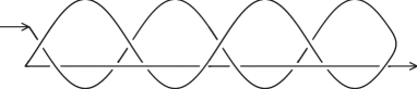
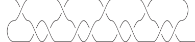
Figure 12: The knot $K_{5}$ is a two-bridge knot

4.2 The harmonic knots $\mathbf{{\rm H}(5,k,k+1).}$

The bridge number of such a knot is at most three, and one can verify that the bridge number of the knots ${\rm H}(5,5k+2,5k+3)$, $\ 2\leq k\leq 8$ is three. This is the reason why the following result surprised us.

Theorem 4.5

The knot ${\rm H}(5,5n+1,5n+2)$ is the two-bridge knot of Conway form $C(2n+1,2n).$
The knot ${\rm H}(5,5n+3,5n+4)$ is the two-bridge knot of Conway form $C(2n+1,2n+2).$
Besides ${\rm H}(5,6,7)={\rm H}(4,5,7)$ and ${\rm H}(5,3,4),$ these knots are not of the form ${\rm H}(a,b,c)$ with $a\leq 4.$

The proof of this result is contained in [KP4]. It is very similar to the preceding one.

4.3 Some new findings on harmonic knots

Thanks to the simplicity of our billiard diagrams, we can easily compute the Alexander polynomials of our knots (see [Li]). On the other hand, there is a list of the Alexander polynomials of the first prime knots with 15 or fewer crossings in [KS].

Using this list and some evident simplifications, we can identify our knot. We first give some specific examples, then an exhaustive list of knots ${\rm H}(a,b,c)$ having a diagram with 15 or fewer crossings.

Harmonic knots are not necessarily prime.
The knot ${\rm H}(5,7,11)$ is not prime; it is the connected sum of two figure-eight knots.

\psfrag{a}{\small$a_{1}$}\psfrag{b}{\small$a_{2}$}\psfrag{c}{\small$a_{n-1}$}\psfrag{d}{\small$a_{n}$}\psfrag{a}{\small$b_{1}$}\psfrag{b}{\small$a_{1}$}\psfrag{c}{\small$c_{1}$}\psfrag{d}{\small$b_{n}$}\psfrag{e}{\small$a_{n}$}\psfrag{f}{\small$c_{n}$}\psfrag{a0}{\small$A^{\prime}_{0}$}\psfrag{b0}{\small$B_{0}$}\psfrag{c0}{\small$C_{0}$}\psfrag{d0}{\small$D_{0}$}\psfrag{an}{\small$A_{n-1}$}\psfrag{bn}{\small$B_{n-1}$}\psfrag{cn}{\small$C^{\prime}_{n-1}$}\psfrag{dn}{\small$D_{n-1}$}\psfrag{aa0}{\small$A_{0}$}\psfrag{cc0}{\small$C^{\prime}_{0}$}\psfrag{aan}{\small$A^{\prime}_{n-1}$}\psfrag{ccn}{\small$C_{n-1}$}\psfrag{aanp}{$A_{n}$}\psfrag{anp}{$A^{\prime}_{n}$}\psfrag{bnp}{$B_{n}$}\psfrag{kn}{$T_{n-1}$}\includegraphics{H5711a.eps}

\psfrag{a}{\small$a_{1}$}\psfrag{b}{\small$a_{2}$}\psfrag{c}{\small$a_{n-1}$}\psfrag{d}{\small$a_{n}$}\psfrag{a}{\small$b_{1}$}\psfrag{b}{\small$a_{1}$}\psfrag{c}{\small$c_{1}$}\psfrag{d}{\small$b_{n}$}\psfrag{e}{\small$a_{n}$}\psfrag{f}{\small$c_{n}$}\psfrag{a0}{\small$A^{\prime}_{0}$}\psfrag{b0}{\small$B_{0}$}\psfrag{c0}{\small$C_{0}$}\psfrag{d0}{\small$D_{0}$}\psfrag{an}{\small$A_{n-1}$}\psfrag{bn}{\small$B_{n-1}$}\psfrag{cn}{\small$C^{\prime}_{n-1}$}\psfrag{dn}{\small$D_{n-1}$}\psfrag{aa0}{\small$A_{0}$}\psfrag{cc0}{\small$C^{\prime}_{0}$}\psfrag{aan}{\small$A^{\prime}_{n-1}$}\psfrag{ccn}{\small$C_{n-1}$}\psfrag{aanp}{$A_{n}$}\psfrag{anp}{$A^{\prime}_{n}$}\psfrag{bnp}{$B_{n}$}\psfrag{kn}{$T_{n-1}$}\includegraphics{H5711b.eps}

Figure 13: The knot ${\rm H}(5,7,11)$ is composite

Harmonic knots may be nonreversible.
We have identified the knots of form ${\rm H}(2n-1,2n+1,2n+3),\ n\leq 5$, by computing their Alexander polynomials and their crossing numbers. We found two nonreversible harmonic knots, namely ${\rm H}(7,9,11)=8_{17}$ and ${\rm H}(9,11,13)=10_{115}.$

Figure 14 shows that ${\rm H}(7,9,11)=8_{17}$ is symmetric through the origin and therefore is strongly ($-$)amphicheiral. It is also the first nonreversible knot (see [Cr, p. 30]).

\psfrag{a}{\small$a_{1}$}\psfrag{b}{\small$a_{2}$}\psfrag{c}{\small$a_{n-1}$}\psfrag{d}{\small$a_{n}$}\psfrag{a}{\small$b_{1}$}\psfrag{b}{\small$a_{1}$}\psfrag{c}{\small$c_{1}$}\psfrag{d}{\small$b_{n}$}\psfrag{e}{\small$a_{n}$}\psfrag{f}{\small$c_{n}$}\psfrag{a0}{\small$A^{\prime}_{0}$}\psfrag{b0}{\small$B_{0}$}\psfrag{c0}{\small$C_{0}$}\psfrag{d0}{\small$D_{0}$}\psfrag{an}{\small$A_{n-1}$}\psfrag{bn}{\small$B_{n-1}$}\psfrag{cn}{\small$C^{\prime}_{n-1}$}\psfrag{dn}{\small$D_{n-1}$}\psfrag{aa0}{\small$A_{0}$}\psfrag{cc0}{\small$C^{\prime}_{0}$}\psfrag{aan}{\small$A^{\prime}_{n-1}$}\psfrag{ccn}{\small$C_{n-1}$}\psfrag{aanp}{$A_{n}$}\psfrag{anp}{$A^{\prime}_{n}$}\psfrag{bnp}{$B_{n}$}\psfrag{kn}{$T_{n-1}$}\includegraphics{HH7911p1.eps}

\psfrag{a}{\small$a_{1}$}\psfrag{b}{\small$a_{2}$}\psfrag{c}{\small$a_{n-1}$}\psfrag{d}{\small$a_{n}$}\psfrag{a}{\small$b_{1}$}\psfrag{b}{\small$a_{1}$}\psfrag{c}{\small$c_{1}$}\psfrag{d}{\small$b_{n}$}\psfrag{e}{\small$a_{n}$}\psfrag{f}{\small$c_{n}$}\psfrag{a0}{\small$A^{\prime}_{0}$}\psfrag{b0}{\small$B_{0}$}\psfrag{c0}{\small$C_{0}$}\psfrag{d0}{\small$D_{0}$}\psfrag{an}{\small$A_{n-1}$}\psfrag{bn}{\small$B_{n-1}$}\psfrag{cn}{\small$C^{\prime}_{n-1}$}\psfrag{dn}{\small$D_{n-1}$}\psfrag{aa0}{\small$A_{0}$}\psfrag{cc0}{\small$C^{\prime}_{0}$}\psfrag{aan}{\small$A^{\prime}_{n-1}$}\psfrag{ccn}{\small$C_{n-1}$}\psfrag{aanp}{$A_{n}$}\psfrag{anp}{$A^{\prime}_{n}$}\psfrag{bnp}{$B_{n}$}\psfrag{kn}{$T_{n-1}$}\includegraphics{HH7911p3.eps}

\psfrag{a}{\small$a_{1}$}\psfrag{b}{\small$a_{2}$}\psfrag{c}{\small$a_{n-1}$}\psfrag{d}{\small$a_{n}$}\psfrag{a}{\small$b_{1}$}\psfrag{b}{\small$a_{1}$}\psfrag{c}{\small$c_{1}$}\psfrag{d}{\small$b_{n}$}\psfrag{e}{\small$a_{n}$}\psfrag{f}{\small$c_{n}$}\psfrag{a0}{\small$A^{\prime}_{0}$}\psfrag{b0}{\small$B_{0}$}\psfrag{c0}{\small$C_{0}$}\psfrag{d0}{\small$D_{0}$}\psfrag{an}{\small$A_{n-1}$}\psfrag{bn}{\small$B_{n-1}$}\psfrag{cn}{\small$C^{\prime}_{n-1}$}\psfrag{dn}{\small$D_{n-1}$}\psfrag{aa0}{\small$A_{0}$}\psfrag{cc0}{\small$C^{\prime}_{0}$}\psfrag{aan}{\small$A^{\prime}_{n-1}$}\psfrag{ccn}{\small$C_{n-1}$}\psfrag{aanp}{$A_{n}$}\psfrag{anp}{$A^{\prime}_{n}$}\psfrag{bnp}{$B_{n}$}\psfrag{kn}{$T_{n-1}$}\includegraphics{HH7911p4.eps}

Figure 14: The knot ${\rm H}(7,9,11),$ an unusual model of $8_{17}$

A table of harmonic knots with $\mathbf{(a-1)(b-1)\leq 30.}$
Here, we provide a table giving the names (up to mirroring) of the knots ${\rm H}(a,b,c)$ with diagrams having $15$ or fewer crossings. The knots are lexicographically ordered, and by Corollary 3.4 we choose $c$ such that $c\not=\lambda a+\mu b,\,\lambda,\mu>0.$ We have to identify 51 knots.

When $a=3$ or $a=4,$ ${\rm H}(a,b,c)$ is a two-bridge knot. The crossing number of such a knot is ${\textstyle{{1}\overwithdelims. .{3}}}(b+c)$, when $a=3$ and ${\textstyle{{1}\overwithdelims. .{4}}}(3b+c-2)$ when $a=4$. Furthermore, its Schubert fraction is computed using Theorem 3.6 or [KP3, Theorem. 6.5].

When $a\geq 5,$ we compute the Alexander polynomial of the knot and compare it with the tables. Sometimes (when starred) it is also necessary to use their DT-notations and Knotscape ([KS]).

Table of the first harmonic knots
	Fraction	Name		Fraction	Name
H(3,4,5)	3	$3_{1}$	H(3,5,7)	5/2	$4_{1}$
H(3,7,8)	5	$5_{1}$	H(3,7,11)	13/5	$6_{3}$
H(3,8,13)	21/8	$7_{7}$	H(3,10,11)	7	$7_{1}$
H(3,10,17)	55/21	$9_{31}$	H(3,11,13)	17/4	$8_{3}$
H(3,11,16)	39/14	$9_{17}$	H(3,11,19)	89/34	$10_{45}$
H(3,13,14)	9	$9_{1}$	H(3,13,17)	53/23	$10_{37}$
H(3,13,20)	105/41	$11a175$	H(3,13,23)	233/89	$12a499$
H(3,14,19)	77/34	$11a119^{*}$	H(3,14,25)	377/144	$13a1739$
H(3,16,17)	11	$11a367$	H(3,16,23)	187/67	$13a2124^{*}$
H(3,16,29)	987/377	$15a39533^{*}$	H(4,5,7)	7/2	$5_{2}$
H(4,5,11)	11/3	$6_{2}$	H(4,7,9)	17/5	$7_{5}$
H(4,7,13)	23/5	$8_{7}$	H(4,7,17)	41/11	$9_{20}$
H(4,9,11)	41/12	$9_{18}$	H(4,9,19)	89/25	$11a180$
H(4,9,23)	153/41	$12a541$	H(4,11,13)	99/29	$11a236$
H(4,11,17)	113/31	$12a758$	H(4,11,21)	187/41	$13a2679^{*}$
H(4,11,25)	329/87	$14a7552^{*}$	H(4,11,29)	571/153	$15a42637^{*}$
H(5,6,7)	7/4	$5_{2}$	H(5,6,13)		$10_{159}$
H(5,6,19)		$10_{116}$	H(5,7,8)	5/2	$4_{1}$
H(5,7,9)	13/8	$6_{3}$	H(5,7,11)		$4_{1}\#4_{1}$
H(5,7,13)		$12n356$	H(5,7,16)		$12n798$
H(5,7,18)		$12n321$	H(5,7,23)		$12a960$
H(5,8,9)	13/4	$7_{3}$	H(5,8,11)	21/13	$7_{7}$
H(5,8,17)		$14n22712^{*}$	H(5,8,19)		$14n26120^{*}$
H(5,8,27)		$14a19221^{*}$	H(6,7,11)		$10_{134}$
H(6,7,17)		$15n42918^{*}$	H(6,7,23)		$15n165258^{*}$
H(6,7,29)		$15a81117$

We have observed that for some integers $b,\,k$ and $h,$ ${\rm H}(b-k,b,b+k)={\rm H}(b-h,b,b+h)$. It is the case for ${\rm H}(5,11,17)={\rm H}(9,11,13)$, ${\rm H}(3,11,19)={\rm H}(7,11,15)$ and many others. It would be interesting to explain this phenomenon.

 

Pierre-Vincent Koseleff,
Université Pierre et Marie Curie (UPMC-Paris 6) & Équipe INRIA Ouragan & Institut de Mathématiques de Jussieu (UMR-CNRS 7586)
e-mail: koseleff@math.jussieu.fr

Daniel Pecker,
Université Pierre et Marie Curie (UPMC-Paris 6) & Institut de Mathématiques de Jussieu (UMR-CNRS 7586)
e-mail: pecker@math.jussieu.fr

References

-
[KA]
D. Bar Nathan, S. Morrison, Knot Atlas, Oct. 2010,
http://katlas.org/wiki/The_Take_Home_Database. - [BDHZ] A. Boocher, J. Daigle, J. Hoste, W. Zheng, Sampling Lissajous and Fourier knots, Exp. Math. 18(4), 481-497 (2009).
- [BHJS] M. G. V. Bogle, J. E. Hearst, V. F. R. Jones, L. Stoilov, Lissajous knots, Journal of Knot Theory and its Ramifications, 3(2): 121-140, (1994).
- [Com] E. H. Comstock, The Real Singularities of Harmonic Curves of three Frequencies, Trans. of the Wisconsin Academy of Sciences, Vol XI : 452-464, (1897).
- [Con] J. H. Conway, An enumeration of knots and links, and some of their algebraic properties, Computational Problems in Abstract Algebra (Proc. Conf., Oxford, 1967), 329–358 Pergamon, Oxford (1970)
- [Cr] P. R. Cromwell, Knots and links, Cambridge University Press, Cambridge, 2004. xviii+328 pp.
- [Fr] G. Freudenburg, Bivariate analogues of Chebyshev polynomials with application to embeddings of affine spaces. Affine algebraic geometry, 39 56, CRM Proc. Lecture Notes, 54, Amer. Math. Soc., Providence, RI, 2011.
-
[KS]
J. Hoste, M. Thistlethwaite, Knotscape,
http://www.math.utk.edu/~morwen/knotscape.html - [HZ] J. Hoste, L. Zirbel, Lissajous knots and knots with Lissajous projections, Kobe Journal of mathematics, vol 24, n, 2007.
- [JP] V. F. R. Jones, J. Przytycki, Lissajous knots and billiard knots, Banach Center Publications, 42:145-163, (1998).
- [Ka] L. Kauffman, On Knots (Princeton University Press, 1987).
- [KP1] P. -V. Koseleff, D. Pecker, On polynomial Torus Knots, Journal of Knot Theory and its Ramifications, Vol. 17 (12) (2008), 1525-1537.
- [KP2] P. -V. Koseleff, D. Pecker, Chebyshev knots, Journal of Knot Theory and its Ramifications, Vol. 20 (4) (2011), 575-593
- [KP3] P. -V. Koseleff, D. Pecker, Chebyshev diagrams for two-bridge knots, Geom. Dedicata 150 (1) , (2011), 405-425.
-
[KP4]
P. -V. Koseleff, D. Pecker, Harmonic Knots,
arXiv:1203.4376 - [KPR] P. -V. Koseleff, D. Pecker, F. Rouillier, The first rational Chebyshev knots, J. Symb. Comput. 45(12), (2010), 1341-1358.
- [La1] C. Lamm, There are infinitely many Lissajous knots, Manuscripta Math., 93: 29-37, (1997).
- [La2] C. Lamm, Zylinder-Knoten und symmetrische Vereinigungen, Dissertation, Universität Bonn, Mathematisches Institut, Bonn, 1999.
- [Li] C. Livingston, Knot Theory, Washington, DC: Math. Assoc. Amer., 1993.
- [Mu] K. Murasugi, Knot Theory and its Applications, Boston, Birkhäuser, 341p., 1996.