Consistent description of nuclear charge radii and electric monopole transitions

Abstract

A systematic study of energy spectra throughout the rare-earth region (even-even nuclei from ₅₈Ce to ₇₄W) is carried out in the framework of the interacting boson model (IBM), leading to an accurate description of the spherical-to-deformed shape transition in the different isotopic chains. The resulting IBM Hamiltonians are then used for the calculation of nuclear charge radii (including isotope and isomer shifts) and electric monopole transitions with consistent operators for the two observables. The main conclusion of this study is that an IBM description of charge radii and electric monopole transitions is possible for most of the nuclei considered but that it breaks down in the tungsten isotopes. It is suggested that this failure is related to hexadecapole deformation.

I Introduction

The structural properties of excited $0^{+}$ states in deformed even-even nuclei have been the subject of a long controversy. According to the geometric model of Bohr and Mottelson Bohr75 , a nucleus with an elipsoidal equilibrium shape may undergo oscillations of two different types, $\beta$ and $\gamma$. The first type of vibration preserves axial symmetry while the second allows excursions toward triaxial shapes. These vibrations should be combined with rotations exhibited by the deformed, vibrating nucleus to yield a rotation-vibration spectrum. The geometric model of Bohr and Mottelson, therefore, predicts an axially deformed nucleus to display a spectrum of rotational bands built on top of vibrational excitations. The lowest in energy is the ground-state rotational band with $K^{\pi}=0^{+}$ (i.e., of which the projection of the angular momentum on the axis of symmetry is zero) which corresponds to no intrinsic excitation. Next in energy are the $\beta$- and $\gamma$-vibrational bands which correspond to one intrinsic excitation of the $\beta$ or $\gamma$ type, characterized by a rotational band with $K^{\pi}=0^{+}$ or $2^{+}$, respectively. At higher energies still, the geometric model predicts rotational bands built on multiple excitations of $\beta$ and/or $\gamma$ phonons.

While $\gamma$-vibrational bands are an acknowledged feature of deformed nuclei, such is not the case for $\beta$-vibrational bands. Confusion arises because excited $0^{+}$ states in nuclei can be of many different characters, such as pairing isomers Ragnarsson76 , two-quasi-particle excitations Soloviev86 , or so-called intruder states that arise through the mechanism of shape coexistence Heyde11 . A careful analysis of the observed properties of excited $0^{+}$ states seems to indicate that very few indeed satisfy all criteria proper to a $\beta$-vibrational state Garrett01 . In particular, although this observation is obfuscated by a lack of reliable data, very few $0^{+}$ states decay to the ground state by way of an electric monopole transition of sizable strength Wood99 , as should be the case for a $\beta$ vibration Reiner61 . It is therefore not surprising that alternative interpretations of excited $0^{+}$ states in deformed nuclei, either as pairing isomers (see, e.g., Refs. Kulp03 ; Kulp05 ) or through shape coexistence and configuration mixing (see, e.g., Ref. Kulp08 ) have gained advocates over recent years.

The purpose of this paper is to examine to what extent a purely collective interpretation of nuclear $0^{+}$ levels is capable of yielding a coherent and consistent description of observed charge radii and electric monopole transitions Zerguine08 . As noted above, very few measured electric monopole transitions satisfy the criteria proper to a matrix element from the ground-state to the $\beta$-vibrational band and the present attempt therefore might seem doomed to failure. However, collective excitations of nuclei can also be described with the interacting boson model (IBM) of Arima and Iachello Arima76 ; Arima78 ; Arima79 , where they are modeled in terms of a constant number of $s$ and $d$ (and sometimes $g$) bosons which can be thought of as correlated pairs of nucleons occupying valence shell-model orbits coupled to angular momentum $\ell=0$ and 2 (and 4), respectively. One of the advantages of the IBM is that a connection with the shell model Otsuka78 as well as with the geometric model Dieperink80 ; Ginocchio80a ; Bohr80 has been established. In particular, one of its dynamical symmetries, the SU(3) limit Arima78 , displays energies reminiscent of the rotation-vibration spectrum of the geometric model. It has also been shown, however, that the first-excited $0^{+}$ state in the SU(3) limit of the IBM has not exactly a $\beta$-vibrational character but is a complicated mixture of intrinsic $\beta$ and $\gamma$ vibrations Casten88 . The main purpose of this paper is to show that a collective interpretation of excited $0^{+}$ states with the IBM is not inconsistent with the electric monopole data, as observed in the rare-earth region.

The outline of this paper as follows. In Sect. II the ground is prepared by discussing charge radii and electric monopole transitions in the context of different models that are applied to even-even nuclei in the rare-earth region from Ce to W in Sect. III. A qualitative explanation of the failure of this approach in the W isotopes is offered in Sect. IV by invoking effects of hexadecapole deformation. Finally, Sect. V summarizes the conclusions of this work.

II Charge radii and electric monopole transitions

Electric monopole (E0) transitions between nuclear levels proceed mainly by internal conversion with no transfer of angular momentum to the ejected electron. If the energy of the transition is greater than $2m_{\rm e}c^{2}$ (where $m_{\rm e}$ is the mass of the electron), they can occur via electron-positron pair creation. A less probable de-excitation mode which can proceed via an E0 transition is two-photon emission. It is not a priori clear why a connection exists between charge radii and E0 transitions. In fact, the argument is rather convoluted and we begin this section by recalling it. The argument can be generalized to effective operators, leading to a relation between charge radii and E0 transitions which forms the basis of the present study.

II.1 Relation between effective operators for charge radii and electric monopole transitions

The total probability for an E0 transition between initial and final states $|{\rm i}\rangle$ and $|{\rm f}\rangle$ can be written as the product of an electronic factor $\Omega$ and a nuclear factor $\rho({\rm E0})$, the latter being equal to Church56

$$\rho({\rm E0})=\langle{\rm f}|\sum_{k\in\pi}\left[\left(\frac{r_{k}}{R}\right)^{2}-\sigma\left(\frac{r_{k}}{R}\right)^{4}+\cdots\right]|{\rm i}\rangle,$$ (1)

with $R=r_{0}A^{1/3}$ and where the summation runs over the $Z$ protons ($\pi$) in the nucleus. The coefficient $\sigma$ depends on the assumed nuclear charge distribution but in any reasonable case it is smaller than 0.1. The second term in Eq. (1) therefore can be neglected if the leading term is not too small Church56 . In this approximation we have

$$\rho({\rm E0})\approx\frac{1}{R^{2}}\langle{\rm f}|\sum_{k\in\pi}r_{k}^{2}|{\rm i}\rangle.$$ (2)

On the other hand, the mean-square charge radius of a state $|{\rm s}\rangle$ is given by

$$\langle r^{2}\rangle_{\rm s}=\frac{1}{Z}\langle{\rm s}|\sum_{k\in\pi}r^{2}_{k}|{\rm s}\rangle.$$ (3)

This is an appropriate expression insofar that a realistic $A$-body wave function is used for the state $|{\rm s}\rangle$. For the heavy nuclei considered here the construction of such realistic wave function is difficult and recourse to an effective charge radius operator $\hat{T}(r^{2})$ should be taken. In particular, if neutrons are assigned an effective charge, the polarization of the protons due to the neutrons is ‘effectively’ taken into account, giving rise to changes in the charge radius $\langle r^{2}\rangle$ with neutron number. The generalization of the expression (3) can therefore be written as

$$\langle r^{2}\rangle_{\rm s} \equiv \langle{\rm s}|\hat{T}(r^{2})|{\rm s}\rangle=\frac{1}{e_{\rm n}N+e_{\rm p}Z}\langle{\rm s}|\sum_{k=1}^{A}e_{k}r^{2}_{k}|{\rm s}\rangle$$ (4)

$$= \frac{1}{e_{\rm n}N+e_{\rm p}Z}\langle{\rm s}|e_{\rm n}\sum_{k\in\nu}r^{2}_{k}+e_{\rm p}\sum_{k\in\pi}r^{2}_{k}|{\rm s}\rangle,$$

where the first summation runs over all $A$ nucleons while the second and third summations run over neutrons ($\nu$) and protons ($\pi$) only, and where $e_{\rm n}$ ($e_{\rm p}$) is the effective neutron (proton) charge. If bare nucleon charges are taken ($e_{\rm n}=0$ and $e_{\rm p}=e$), the summation extends over protons only and the original expression (3) is recovered. If equal nucleon charges are taken ($e_{\rm n}=e_{\rm p}$), Eq. (4) is appropriate for the matter radius.

In the approximation $\sigma\approx 0$, the starting expressions (2) and (3) for the nuclear E0 transition strength and the mean-square charge radius are identical (up to the constants $R^{2}$ and $Z$). It is therefore natural to follow the same argument as used for the charge radius for the construction of a generalized E0 transition operator, leading to the expression Kantele84

$$\hat{T}({\rm E0})=\sum_{k=1}^{A}e_{k}r^{2}_{k}=e_{\rm n}\sum_{k\in\nu}r^{2}_{k}+e_{\rm p}\sum_{k\in\pi}r^{2}_{k}.$$ (5)

In terms of this operator, the dimensionless quantity $\rho({\rm E0})$, defined in Eq. (2) and referred to as the monopole strength, is given by

$$\rho({\rm E0})=\frac{\langle{\rm f}|\hat{T}({\rm E0})|{\rm i}\rangle}{eR^{2}}.$$ (6)

Since the matrix element (6) is known up to a sign only, usually $\rho^{2}({\rm E0})$ is quoted.

The basic hypothesis of the present study is to assume that the effective nucleon charges in the charge radius and E0 transition operators are the same. If this is so, comparison of Eqs. (4) and (5) leads to the relation

$$\hat{T}({\rm E0})=(e_{\rm n}N+e_{\rm p}Z)\hat{T}(r^{2}).$$ (7)

This is a general relation between the effective operators used for the calculation of charge radii and E0 transitions, which is applied throughout this study.

II.2 Charge radii and electric monopole transitions in the interacting boson model

Equation (7) can, in principle, be tested in the framework of any model. This endeavor is difficult in the context of the nuclear shell model because realistic wave functions, appropriate for the calculation of $\langle r^{2}\rangle$ or E0 matrix elements, are hard to come by for heavy nuclei. As an alternative we propose here to test the implied correlation with the use of a simpler model, namely the IBM Arima76 ; Arima78 ; Arima79 . This requires that all states involved [i.e., $|{\rm s}\rangle$ in Eq. (4), and $|{\rm i}\rangle$ and $|{\rm f}\rangle$ in Eq. (6)] are collective in character and can be described by the IBM.

In the IBM-1, where no distinction is made between neutron and proton bosons, the charge radius operator is taken as the most general scalar expression that is linear in the generators of U(6) Iachello87 ,

$$\hat{T}(r^{2})=\langle r^{2}\rangle_{\rm c}+\alpha N_{\rm b}+\eta\frac{\hat{n}_{d}}{N_{\rm b}},$$ (8)

where $N_{\rm b}$ is the total boson number (the customary notation $N$ is not used here to avoid confusion with the neutron number), $\hat{n}_{d}$ is the $d$-boson number operator, and $\alpha$, $\eta$ are parameters with units of length². The first term in Eq. (8), $\langle r^{2}\rangle_{\rm c}$, is the charge radius of the core nucleus. The second term accounts for the (locally linear) increase in the charge radius due to the addition of two nucleons (i.e., neutrons since isotope shifts are considered in this study). The boson number $N_{\rm b}$ is the number of pairs of valence particles or holes (whichever is smaller) counted from the nearest closed shells for neutrons and protons. If the bosons are particle-like, the addition of two nucleons corresponds to an increase of $N_{\rm b}$ by one and $\alpha$ is positive. In contrast, if the bosons are hole-like, the addition of two nucleons corresponds to a decrease of $N_{\rm b}$ by one and $\alpha$ is negative. Therefore, care should be taken to change the sign of $\alpha$ at mid-shell Iachello87 . The third term in Eq. (8) stands for the contribution to the charge radius due to deformation. It is identical to the one given in Ref. Iachello87 but for the factor $1/N_{\rm b}$. This factor is included here because it is the fraction $\langle\hat{n}_{d}\rangle/N_{\rm b}$ which is a measure of the quadrupole deformation ($\beta_{2}^{2}$ in the geometric collective model) rather than the matrix element $\langle\hat{n}_{d}\rangle$ itself. Since the inclusion of $1/N_{\rm b}$ is non-standard, also results without this factor will be given in the following, that is, with the charge radius operator

$$\hat{T}^{\prime}(r^{2})=\langle r^{2}\rangle_{\rm c}+\alpha^{\prime}N_{\rm b}+\eta^{\prime}\hat{n}_{d}.$$ (9)

Once the form of the charge radius operator is determined, that of the E0 transition operator follows from Eq. (7). In the IBM-1 the E0 transition operators are therefore

$$\hat{T}({\rm E0})=(e_{\rm n}N+e_{\rm p}Z)\eta\frac{\hat{n}_{d}}{N_{\rm b}},$$ (10)

or

$$\hat{T}^{\prime}({\rm E0})=(e_{\rm n}N+e_{\rm p}Z)\eta^{\prime}\hat{n}_{d}.$$ (11)

Since for E0 transitions the initial and final states are different, neither the constant $\langle r^{2}\rangle_{\rm c}$ nor $\alpha N_{\rm b}$ in Eq. (8) or $\alpha^{\prime}N_{\rm b}$ in Eq. (9) contribute to the transition, so they can be omitted from the E0 operators.

Two other quantities can be derived from charge radii, namely isotope and isomer shifts. The former measures the difference in charge radius of neighboring isotopes. For the difference between even-even isotopes one finds from Eq. (8)

$$\Delta\langle r^{2}\rangle^{(A)} \equiv \langle r^{2}\rangle_{0_{1}^{+}}^{(A+2)}-\langle r^{2}\rangle_{0_{1}^{+}}^{(A)}$$ (12)

$$= |\alpha|+\eta\left(\langle\frac{\hat{n}_{d}}{N_{\rm b}}\rangle_{0_{1}^{+}}^{(A+2)}-\langle\frac{\hat{n}_{d}}{N_{\rm b}}\rangle_{0_{1}^{+}}^{(A)}\right).$$

The occurrence of the absolute value $|\alpha|$ is due to the interpretation of the bosons as pairs of particles or holes, as discussed above. Isomer shifts are a measure of the difference in charge radius between an excited (here the $2_{1}^{+}$) state and the ground state, and are given by

$$\delta\langle r^{2}\rangle^{(A)} \equiv \langle r^{2}\rangle^{(A)}_{2_{1}^{+}}-\langle r^{2}\rangle^{(A)}_{0_{1}^{+}}$$ (13)

$$= \eta\left(\langle\frac{\hat{n}_{d}}{N_{\rm b}}\rangle_{2_{1}^{+}}^{(A)}-\langle\frac{\hat{n}_{d}}{N_{\rm b}}\rangle_{0_{1}^{+}}^{(A)}\right).$$

Similar formulas hold for the charge radius operator (9) in terms of the parameters $\alpha^{\prime}$ and $\eta^{\prime}$. For ease of notation, the superscript $(A)$ in the isotope and isomer shifts shall be suppressed in the following.

II.3 Estimate of the coefficients $\alpha$ and $\eta$

Although the coefficients $\alpha$ and $\eta$ in Eq. (8) will be treated as parameters and fitted to data on charge radii and E0 transitions, it is important to have an estimate of their order of magnitude. The term in $\alpha$ increases with particle number and therefore can be associated with the ‘standard’ isotope shift. This standard contribution to the charge radius is given by Bohr69

$$\langle r^{2}\rangle^{(A)}_{0_{1}^{+},{\rm std}}\approx\frac{3}{5}r_{0}^{2}A^{2/3}.$$ (14)

The term in $\eta$ stands for the contribution to the nuclear radius due to deformation. For a quadrupole deformation it is estimated to be Bohr69

$$\langle r^{2}\rangle^{(A)}_{0_{1}^{+},{\rm def}}\approx\frac{5}{4\pi}\beta_{2}^{2}\langle r^{2}\rangle^{(A)}_{0_{1}^{+},{\rm std}}\approx\frac{3}{4\pi}\beta_{2}^{2}r_{0}^{2}A^{2/3},$$ (15)

where $\beta_{2}$ is the quadrupole deformation parameter of the geometric model.

The estimate of $|\alpha|$ follows from

$$|\alpha| = \Delta\langle r^{2}\rangle^{(A)}_{\rm std}\approx\frac{3}{5}r_{0}^{2}\left((A+2)^{2/3}-A^{2/3}\right)$$ (16)

$$\approx \frac{4}{5}r_{0}^{2}A^{-1/3},$$

which for the nuclei considered here ($A\sim 150$) gives $|\alpha|\approx 0.2$ fm². The estimate of $\eta$ can be obtained by associating the deformation contribution (15) with the expectation value of $\langle\hat{n}_{d}\rangle_{0^{+}_{1}}$ in the IBM. This leads to the relation

$$\eta\frac{{\bar{\beta}_{2}}^{2}}{1+{\bar{\beta}_{2}}^{2}}\approx\frac{4}{3}{\bar{\beta}_{2}}^{2}r_{0}^{2}N_{\rm b}^{2}A^{-4/3},$$ (17)

where use has been made of the approximate correspondence $\beta_{2}\approx(4N_{\rm b}/3A)\sqrt{\pi}\bar{\beta}_{2}$ between the quadrupole deformations $\beta_{2}$ and $\bar{\beta}_{2}$ in the geometric model and in the IBM, respectively Ginocchio80b . The relation (17) yields the estimate

$$\eta\approx\frac{4}{3}(1+{\bar{\beta}_{2}}^{2})r_{0}^{2}N_{\rm b}^{2}A^{-4/3}.$$ (18)

For typical values of $N_{\rm b}\sim 10$ and $A\sim 150$ this gives a range of possible $\eta$ values between 0.25 and 0.75 fm², corresponding to weakly deformed ($\bar{\beta}_{2}\ll 1$) and strongly deformed ($\bar{\beta}_{2}\approx\sqrt{2}$) nuclei, respectively.

Similar estimates can be derived for the coefficients in the alternative form (9) of the charge radius operator. The estimate for $|\alpha^{\prime}|$ is identical to Eq. (16) while the one for $\eta^{\prime}$ differs by a factor $N_{\rm b}$.

II.4 Estimate of the effective charges

The consistent definition of operators for charge radii and E0 transitions leads to the introduction of neutron and proton effective charges for both operators, as opposed to previous treatments where this was done for E0 transitions only. This opens the possibility to obtain an estimate of the effective charges $e_{\rm n}$ and $e_{\rm p}$ from data for charge radii which are widely available.

A simple estimate can be obtained in a Hartree-Fock approximation with harmonic-oscillator single-particle wave functions. For the Hartree-Fock ground state $|{\rm gs}\rangle$ of a nucleus, simple counting arguments of the degeneracies of the three-dimensional harmonic oscillator (see Sect. 2.2 of Ref. Brussaard77 ), lead to the following expression for the expectation value of the neutron part of the charge radius operator:

$$\langle{\rm gs}|\sum_{k\in\nu}r^{2}_{k}|{\rm gs}\rangle=\frac{3^{4/3}}{4}N^{4/3}b^{2}=\frac{3\cdot 2^{1/3}}{5}r_{0}^{2}N^{4/3}A^{1/3},$$ (19)

where $b$ is the oscillator length of the harmonic oscillator for which the estimate $b=2^{7/6}3^{-1/6}5^{-1/2}r_{0}A^{1/6}$ is used Brussaard77 . Equation (19) and its equivalent for the proton part of the charge radius operator, can then be combined to yield

$$\langle r^{2}\rangle_{\rm gs}=\frac{3\cdot 2^{1/3}}{5}r_{0}^{2}\frac{(e_{\rm n}N^{4/3}+e_{\rm p}Z^{4/3})A^{1/3}}{e_{\rm n}N+e_{\rm p}Z}.$$ (20)

The separate effective charges $e_{\rm n}$ and $e_{\rm p}$ cannot be obtained from a fit of this expression to the data on charge radii, but the ratio $e_{\rm n}/e_{\rm p}$ can. There exists, unfortunately, a strong dependence of this ratio on the value used for $r_{0}$, as will be discussed in Subsect. III.3.

II.5 Relating charge radii and electric monopole transitions through configuration mixing

The idea of correlating observed E0 transitions with charge radii is not new and, in particular, was already proposed by Wood et al. Wood99 . These authors tested this proposal in the context of a model assuming mixing between two different coexisting configurations. Since in Sect. III results are quoted for the few nuclei where this model has been applied, a brief reminder of the method is given in this subsection.

Assume that the initial and final levels in the E0 transition are orthogonal mixtures of some states $|\alpha_{1}J\rangle$ and $|\alpha_{2}J\rangle$, so that

$$|{\rm i}J\rangle = a_{J}|\alpha_{1}J\rangle+b_{J}|\alpha_{2}J\rangle,$$

$$|{\rm f}J\rangle = a_{J}|\alpha_{2}J\rangle-b_{J}|\alpha_{1}J\rangle.$$ (21)

The labels $\alpha_{1}$ and $\alpha_{2}$ refer to a different intrinsic structure for the two sets of states (typically two bands), the members of which are additionally characterized by their angular momentum $J$. The $a_{J}$ and $b_{J}$ are mixing coefficients that satisfy $a_{J}^{2}+b_{J}^{2}=1$. If one assumes that no E0 transition is allowed between states with a different intrinsic structure, $\langle\alpha_{1}J|\hat{T}({\rm E0})|\alpha_{2}J\rangle\approx 0$, it follows that

$$\langle{\rm f}J|\hat{T}({\rm E0})|{\rm i}J\rangle$$ (22)

$$\approx a_{J}b_{J}\left(\langle\alpha_{2}J|\hat{T}({\rm E0})|\alpha_{2}J\rangle-\langle\alpha_{1}J|\hat{T}({\rm E0})|\alpha_{1}J\rangle\right)$$

$$= a_{J}b_{J}(e_{\rm n}N+e_{\rm p}Z)\left(\langle r^{2}\rangle_{\alpha_{2}J}-\langle r^{2}\rangle_{\alpha_{1}J}\right),$$

where the last equality is due to Eq. (7). Furthermore, it must be hoped that the difference in $\langle r^{2}\rangle$ appearing in Eq. (22) can be identified with a measured isotope shift $\Delta\langle r^{2}\rangle$ between nuclei somewhere in the neighborhood and, therefore, that the ground states of two nuclei in the neighborhood can be identified with the unmixed intrinsic structures $\alpha_{1}$ and $\alpha_{2}$. Finally, it must be assumed that this difference in $\langle r^{2}\rangle$ does not depend significantly on $J$ or, equivalently, that isomer shifts are identical for the intrinsic structures $\alpha_{1}$ and $\alpha_{2}$. With this first set of assumptions the following relation holds:

$$\rho^{2}_{J}({\rm E0})=a_{J}^{2}b_{J}^{2}\frac{(e_{\rm n}N+e_{\rm p}Z)^{2}}{e^{2}R^{4}}[\Delta\langle r^{2}\rangle]^{2},$$ (23)

which reduces to the result of Wood et al. Wood99 if bare nucleon charges are taken. According to this equation the $J$ dependence of the E0 strength is contained in the coefficients $a_{J}$ and $b_{J}$, which can be obtained from a two-state mixing calculation. An additional input into the calculation, therefore, is the relative position in energy of the intrinsic structures $\alpha_{1}$ and $\alpha_{2}$ and the size of the mixing matrix element (itself assumed to be independent of $J$). These are the essential ingredients of the calculations reported by Kulp et al. Kulp08 of which the results are quoted below.

III Systematic study of nuclei in the rare-earth region

To test the relation between charge radii and E0 transitions, proposed in the previous section, a systematic study of all even-even isotopic chains from Ce to W is carried out. This analysis requires the knowledge of structural information concerning the ground states and excited states which here is obtained by adjusting an IBM-1 Hamiltonian to observed spectra in the rare-earth region.

III.1 Hamiltonian and energy spectra

All isotope series in the rare-earth region from $Z=58$ to $Z=74$ have the particularity to vary from spherical to deformed shapes and to display systematically a shape phase transition. Such nuclear behavior can be parametrized in terms of a simplified IBM-1 Hamiltonian which can be represented on the so-called Casten triangle Casten81 , as demonstrated for rare-earth nuclei by Mc Cutchan et al. Cutchan04 . Alternatively, as shown by García-Ramos et al. Garcia03 , the same region of the nuclear chart can be described with the full IBM Hamiltonian. The latter approach is adopted here and a general one- and two-body Hamiltonian is considered which is written in multipole form as Iachello87

$$\hat{H}=\epsilon_{d}\hat{n}_{d}+a_{0}\hat{P}_{+}\cdot\hat{P}_{-}+a_{1}\hat{L}\cdot\hat{L}+a_{2}\hat{Q}\cdot\hat{Q}+a_{3}\hat{T}_{3}\cdot\hat{T}_{3}+a_{4}\hat{T}_{4}\cdot\hat{T}_{4},$$ (24)

where $\hat{n}_{d}$ is the $d$-boson number operator, $\hat{P}_{+}$ ($\hat{P}_{-}$) is a boson-pair creation (annihilation) operator, $\hat{L}$ is the angular momentum operator, and $\hat{Q}$, $\hat{T}_{3}$, and $\hat{T}_{4}$ are quadrupole, octupole, and hexadecapole operators, respectively. (For the definitions of these operators in terms of $s$ and $d$ bosons, see Sect. 1.4.7 of Iachello and Arima Iachello87 .) If only excitation and no absolute energies are considered, the expression (24) defines the most general Hamiltonian with one- and two-body interactions between the bosons in terms of six parameters. The parameter $\chi$ in the quadrupole operator $\hat{Q}$ can be arbitrarily chosen (as long as it is different from zero) and is fixed here to $-\sqrt{7}/2$ for all nuclei.

Although reasonable results are obtained with constant parameters for an entire chain of isotopes, the spherical-to-deformed transition is better described if at least one parameter is allowed to vary with boson number $N_{\rm b}$. García-Ramos et al. Garcia03 followed the procedure to vary the $d$-boson energy $\epsilon_{d}$ with $N_{\rm b}$. A different method is followed here by allowing the variation of the coefficient $a_{2}$ associated with the quadrupole term. To reduce the number of parameters in the fit, we assume that $a_{2}$ depends linearly on the quantity $N_{\nu}N_{\pi}/(N_{\nu}+N_{\pi})$ where $N_{\nu}$ ($N_{\pi}$) is half the number of valence neutrons (protons) particles or holes, whichever is smaller. The argument for introducing such a dependence is related to the importance of the neutron-proton interaction as the deformation-driving mechanism in nuclei Casten85 . The parameter $a_{2}$ can then be decomposed into two terms as follows:

$$a_{2}=a^{\prime}_{2}+\frac{N_{\nu}N_{\pi}}{N_{\nu}+N_{\pi}}a^{\prime\prime}_{2}.$$ (25)

Table 1: Parameters in the Hamiltonian (24) and the rms deviation $\sigma$, in units of keV.

Isotopes		$\epsilon_{d}$	$a_{0}$	$a_{1}$	$a^{\prime}_{2}$	$a^{\prime\prime}_{2}$	$a_{3}$	$a_{4}$		$\sigma$
${}^{144-152}_{\phantom{000-0}58}$Ce		$1516.9$	$67.7$	$-8.6$	$-26.5$	$-2.2$	$-185.9$	$-113.1$		$81$
${}^{146-156}_{\phantom{000-0}60}$Nd		$1701.0$	$55.9$	$-16.2$	$-17.2$	$-0.6$	$-78.1$	$-221.5$		$124$
${}^{148-160}_{\phantom{000-0}62}$Sm		$944.2$	$-73.7$	$5.7$	$-0.2$	$-15.2$	$-227.4$	$70.0$		$107$
${}^{150-162}_{\phantom{000-0}64}$Gd		$1857.2$	$69.1$	$-15.3$	$-8.4$	$-1.7$	$-52.8$	$-228.0$		$115$
${}^{152-164}_{\phantom{000-0}66}$Dy		$1887.2$	$75.6$	$-12.3$	$-8.8$	$-0.7$	$-53.5$	$-219.2$		$97$
${}^{154-170}_{\phantom{000-0}68}$Er		$1772.6$	$105.9$	$-10.9$	$-6.7$	$-0.9$	$-43.5$	$-222.0$		$87$
${}^{156-176}_{\phantom{000-0}70}$Yb		$780.4$	$43.5$	$0.5$	$6.7$	$-5.2$	$-20.9$	$-41.4$		$91$
${}^{160-182}_{\phantom{000-0}72}$Hf		$1061.7$	$62.5$	$-7.0$	$-7.0$	$-0.2$	$36.0$	$-128.2$		$103$
${}^{164-190}_{\phantom{000-0}74}$W		$1068.4$	$73.0$	$-3.8$	$-7.0$	$-0.5$	$5.7$	$-136.7$		$103$

The parameters in the Hamiltonian (24) are determined from a least-squares fit to levels of the ground-state band with $K^{\pi}=0^{+}$ and those of two more bands with $K^{\pi}=0^{+}$ and $K^{\pi}=2^{+}$ (‘quasi-$\beta$’ and ‘quasi-$\gamma$’ bands). Since two-quasi-particle excitations do not belong to the model space of the IBM-1, states beyond the backbend cannot be described in this version of the model and for this reason only levels up to $J^{\pi}=10^{+}$ are included in the fit. Similarly, near closed shells, excitations might be of single-particle character and, therefore, nuclei with $N\leq 84$ are excluded from the energy fit. Nevertheless, the Hamiltonian (24) with the parametrization (25) allows the extrapolation toward the $N=84$ isotopes, which is needed for some of the isotope shifts calculated in the following. The total number of nuclei included in the fit is 78 and the total number of excited levels is 846. The parameters are summarized in Table 1 as well as the root-mean-square (rms) deviation $\sigma$ for each isotope chain which typically is of the order of 100 keV.

Figure 1: Experimental (points) and calculated (lines) energy levels in the Sm, Gd, and Dy isotopes: (a) ground-state band up to $J^{\pi}=10^{+}$, (b) first-excited $K^{\pi}=0^{+}$ band up to $J^{\pi}=4^{+}$, and (c) first-excited $K^{\pi}=2^{+}$ band up to $J^{\pi}=4^{+}$.

Figure 1 illustrates, with the examples of samarium, gadolinium, and dysprosium, the typical evolution of the energy spectrum of a spherical to that of a deformed nucleus which is observed for every isotope series studied here. In each nucleus are shown levels of the ground-state band up to angular momentum $J^{\pi}=10^{+}$ as well as the first few states of the excited bands, together with their experimental counterparts, if known.

For a given nucleus the choice of the subset of collective states that should be included in the fit is often far from obvious. While members of the ground-state and the $\gamma$-vibrational bands in a deformed nucleus are readily identified, this is not necessarily so for the ‘$\beta$-vibrational’ band. As a result, guided by the E0 transitions discussed in the next subsection, the calculated first-excited $K^{\pi}=0^{+}$ band is associated in some nuclei not with the lowest observed $K^{\pi}=0^{+}$ band but with a higher-lying one. This is the case for ^168-172Yb and also for ¹⁶⁶Er where the fourth $J^{\pi}=0^{+}$ level at 1934 keV has been recently identified as the band head of the $\beta$-vibrational band on the basis of its large E0 matrix element to the ground state Wimmer09 .

Although the agreement with the experiment can be called satisfactory, it should be noted from Table 1 that it is obtained with rather large parameter fluctuations between the different isotopic chains. This presumably is so because the parameters are highly correlated and small changes in the fitted data give rise to large fluctuations in some of the parameters. The main purpose of this calculation, however, is not to establish some parameter systematics with the Hamiltonian (24) but rather to arrive at a reasonably realistic description of the spherical-to-deformed transition. This will enable a simultaneous calculation of charge radii and E0 transitions, as discussed in the next two subsections.

III.2 Isotope and isomer shifts

Table 2: The parameters $|\alpha|$ and $|\alpha^{\prime}|$ in the charge radius operators (8) and (9), in units of fm², for the different isotope series.

Isotope	Ce	Nd	Sm	Gd	Dy	Er	Yb	Hf	W
$|\alpha|$	0.22	0.24	0.26	0.13	0.15	0.15	0.11	0.10	0.11
$|\alpha^{\prime}|$	0.23	0.25	0.26	0.09	0.12	0.12	0.09	0.11	0.15

Isotope shifts $\Delta\langle r^{2}\rangle$, according to Eq. (12), depend on the parameters $|\alpha|$ and $\eta$ in the IBM-1 operator (8). These parameters are expected to vary smoothly with mass number $A$, according to Eqs. (16) and (18). The estimate (16) neglects, however, the microscopic make-up of the pair of neutrons which varies considerably from Ce to W. It is therefore necessary to adjust $|\alpha|$ for each isotope series separately, and the resulting values are given in the first row of Table 2. The value of $\eta$, on the other hand, is kept constant for all isotopes, $\eta=0.50$ fm². The parameters thus derived are broadly consistent with the estimates obtained in Subsect. II.3.

Similar remarks hold for the alternative parametrization (9) of the charge radius operator. The values of $|\alpha^{\prime}|$ are given in the second row of Table 2 while $\eta^{\prime}=0.05$ fm².

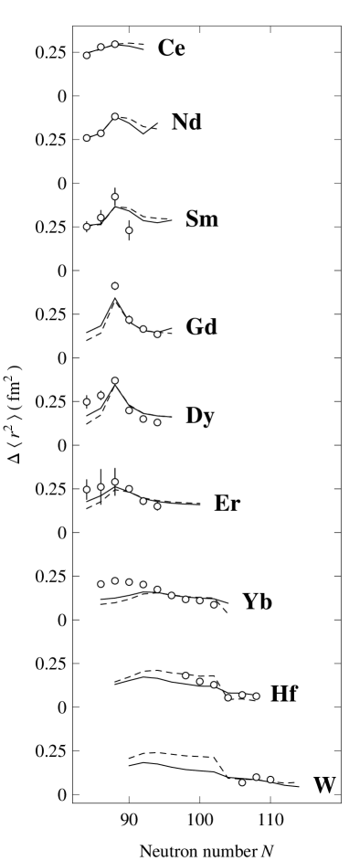
Figure 2: Experimental (points) and calculated (lines) isotope shifts $\Delta\langle r^{2}\rangle$, in units of fm², for isotopic chains in the rare-earth region from Ce to W. The full (dashed) lines are for the charge radius operator (8) [(9)], with parameters given in Table 2 and in the text. Data are taken from Ref. Cheal03 for Ce, from Ref. Otten89 for Nd, Sm, Dy, Er, and Yb, from Ref. Frick95 for Gd, from Ref. Angeli04 for Hf, and from Ref. Jin94 for W.

The resulting isotope shifts are shown in Fig. 2. Only mariginal differences exist between the two sets of calculations, with and without the factor $1/N_{\rm b}$ in the charge radius operator. The main reason for preferring the form (8) is that it lacks a kink in $\Delta\langle r^{2}\rangle$ at mid-shell. Although this seems to occur in the Hf data, it is unlikely that the observed kink is associated with a maximum of the boson number at mid-shell. Given the similarity between the two sets of calculations, the subsequent comments are valid for both.

The peaks in the isotope shifts are well reproduced in all isotopic chains with the exception of Yb. The largest peaks occur for ^152-150Sm, ^154-152Gd, and ^156-154Dy, that is, for the difference in radii between $N=90$ and $N=88$ isotopes. The peak is smaller below $Z=62$ for Ce and Nd, and fades away above $Z=66$ for Er, Yb, Hf, and W. The calculated isotope shifts broadly agree with these observed features but there are differences though. Notably, the calculated peak in the Sm isotopes is much broader than the observed one, indicating that the spherical-to-deformed transition occurs faster in reality than it does in the IBM-1 calculation. Also, it would be of interest to determine the character of the transition in the Nd isotopes: the present IBM-1 calculation predicts it to be rather smooth but data in the deformed region of the transition are lacking to confirm this behavior. Likewise, the IBM-1 calculation features a very fast transition for the Gd isotopes with a sharp peak at $N=88$ but isotope-shift data are lacking for the nuclei in the spherical region of the transition.

The feature of peaking isotope shifts is related to the onset of deformation which is particularly sudden (as a function of neutron number) for the Sm, Gd, and Dy isotopes. This can be quantitatively understood as a result of the subshell closure at $Z=64$ Ogawa78 , combined with the strongly attractive interaction between neutrons in the $1\nu h_{9/2}$ orbit and protons in the $1\pi h_{11/2}$ orbit. If the occupancies of the neutrons in the $1\nu h_{9/2}$ and of the protons in the $1\pi h_{11/2}$ orbit are both low, as is the case for $N\leq 92$ and $Z\leq 64$, the nucleus is expected to be spherical. As soon as one of the two orbits becomes significantly occupied, the strong neutron-proton interaction will induce occupancy of the partner orbit and an onset of deformation.

Table 3: Experimental and calculated isomer shifts $\delta\langle r^{2}\rangle$, in units of $10^{-3}$ fm², in the rare-earth region.

			$\delta\langle r^{2}\rangle$ ($10^{-3}$ fm2)
Isotope			Th1		Th2		Th3		Expt			Ref
150Sm			80		72				49.6	2.6		Yamazaki78
152Sm			37		37		19		25.00	7.		Yeboah67
									19.00			Steiner67
									14.00	1.		Bernow68
									12.00			Baader68
									18.00	4.		Yamazaki78
154Sm			6		7				1.100	0.8		Wheeler70
154Gd			28		31				15.00	2.		Bernow68
									19.00	6.		Rehm69
									18.5	2.5		Backe74
									20.0	3.9		Laubacher83
156Gd			4		5				2.6	0.8		Henning68
									0.1	1.7		Backe74
									4.3	3.7		Laubacher83
158Gd			3		4				0.4	0.3		Fink67
									1.5	0.8		Russell70
									$-4.0$	1.2		Backe74
									0.3	3.3		Laubacher83
160Gd			1		1				0.3	0.8		Russell70
									$-1.4$	3.1		Backe74
									$-2.1$	3.2		Laubacher83
170Yb			4		6				1.2	0.3		Henning68
									1.7	0.6		Henning71
									1.20	0.40		Russell73
172Yb			3		5				0.41	0.20		Russell73
174Yb			2		4				1.0	0.45		Henning71
									$-0.44$	0.19		Russell73
176Yb			2		4				$-0.17$	0.10		Russell73
182W			5		6				6.0			Cohen66
									$-0.6$			Baader68
									$-0.2$			Wagner71
184W			8		9				0.16			Wagner71
									0.5	0.3		Hardy71
186W			17		18				0.14			Wagner71

A further test of the calculated charge radii is obtained from isomer shifts $\delta\langle r^{2}\rangle$, depending only on $\eta$ [see Eq. (13)] or $\eta^{\prime}$. The isomer shifts that are known experimentally are listed in Table 3. The data are more than 30 years old and often discrepant. Nevertheless, a clear conclusion can be drawn from the isomer shifts measured in the Sm and Gd isotopes: they are easily an order of magnitude smaller in the deformed than they are in the spherical region. In spite of the extreme sensitivity of this effect, a quantitative description is obtained of the isomer shifts in the Gd isotopes. For the Sm isotopes only a qualitative agreement is found since the experimentally observed drop in isomer shift between ¹⁵²Sm and ¹⁵⁴Sm is stronger than what is calculated in the IBM-1. This indicates that the spherical-to-deformed transition is faster in reality than it is in the calculation, in line with what can be concluded from the isotope shifts.

From the preceding analysis the following picture emerges. All considered isotopic chains exhibit an evolution from a spherical to a deformed shape which, at the phase-transitional point, is characterized by a peak in the isotope shifts. The height of the peak is proportional to the suddenness of the transition. This effect is a direct consequence of the increase in the mean-square radius of a nucleus due to its deformation. The IBM-1 is able to provide an adequate description of this transitional behavior. By adjusting the charge radius operator of the IBM-1 to the observed height of the peak in the isotope shifts, a first estimate of the parameter $\eta$ (or $\eta^{\prime}$) is obtained. Its value follows more directly from isomer shifts since only one parameter enters this quantity but, unfortunately, data are scarce and often unreliable. The choice $\eta=0.50$ fm² (or $\eta^{\prime}=0.05$ fm²) is a compromise between the value obtained from a fit to $\Delta\langle r^{2}\rangle$ of all isotopes and the one from $\delta\langle r^{2}\rangle$ in the Gd isotopes. The question is now whether this value of $\eta$ (or $\eta^{\prime}$) reproduces the E0 transitions observed in the rare-earth nuclei.

III.3 Electric monopole transitions

The calculation of the matrix elements of the E0 transition operator (10) or (11) requires the knowledge of the effective charges $e_{\rm n}$ and $e_{\rm p}$. In principle, an estimate of the ratio $e_{\rm n}/e_{\rm p}$ can be obtained by fitting the expression (20) to the available data on charge radii in the rare-earth region. The minimum in the rms deviation is shallow though and, furthermore, the correlation between $r_{0}$ and $e_{\rm n}/e_{\rm p}$ is strong. In other words, a slightly different choice of $r_{0}$ gives an almost equally good fit to the charge radii of $58\leq Z\leq 74$ nuclei but with a significantly different ratio $e_{\rm n}/e_{\rm p}$. A reasonable choice of parameters, close to the optimum set, corresponds to $r_{0}=1.24$ fm, $e_{\rm n}=0.50e$, and $e_{\rm p}=e$.

Table 4: Experimental and calculated $\rho^{2}({\rm E0})$ values in the rare-earth region.

											$\rho^{2}({\rm E0})\times 10^{3}$
Isotope			Transition					$J$			Th1		Th2		Th3		Expt
150Sm			740	$\rightarrow$	0			0			7		6				18	2
			1046	$\rightarrow$	334			2			16		13				100	40
152Sm			685	$\rightarrow$	0			0			52		52		72		51	5
			811	$\rightarrow$	122			2			41		41		77		69	6
			1023	$\rightarrow$	366			4			29		29		84		88	14
			1083	$\rightarrow$	0			0			2		2				0.7	0.4
			1083	$\rightarrow$	685			0			47		47				22	9
154Sm			1099	$\rightarrow$	0			0			41		49				96	42
152Gd			615	$\rightarrow$	0			0			68		68				63	14
			931	$\rightarrow$	344			2			77		77				35	3
154Gd			681	$\rightarrow$	0			0			84		102				89	17
			815	$\rightarrow$	123			2			66		80				74	9
			1061	$\rightarrow$	361			4			38		46				70	7
156Gd			1049	$\rightarrow$	0			0			44		64				42	20
			1129	$\rightarrow$	89			2			41		59				55	5
158Gd			1452	$\rightarrow$	0			0			30		51				35	12
			1517	$\rightarrow$	79			2			27		45				17	3
158Dy			1086	$\rightarrow$	99			2			42		70				27	12
160Dy			1350	$\rightarrow$	87			2			28		56				17	4
162Er			1171	$\rightarrow$	102			2			38		64				630	460
164Er			1484	$\rightarrow$	91			2			24		48				90	50
166Er			1460	$\rightarrow$	0			0			9		20				127	60
170Yb			1229	$\rightarrow$	0			0			32		72				27	5
172Yb			1405	$\rightarrow$	0			0			30		76				0.2	0.03
174Hf			900	$\rightarrow$	91			2			32		71				27	13
176Hf			1227	$\rightarrow$	89			2			15		38				52	9
178Hf			1496	$\rightarrow$	93			2			32		72				14	3
182W			1257	$\rightarrow$	100			2			45		77				3.5	0.3
184W			1121	$\rightarrow$	111			2			52		75				2.6	0.5

In Table 4 the available E0 data in the rare-earth region are compared with the results of this calculation. The two choices of E0 transition operator, Eqs. (10) and (11), again yield comparable results. An overall comment is that the present approach succeeds in reproducing the correct order of magnitude for $\rho^{2}({\rm E}0)$, in particular in the Sm, Gd, and Dy isotopes. However, some discrepancies can be observed in heavier nuclei and especially concern ¹⁷²Yb and ^182-184W. A possible explanation is that the $\rho^{2}({\rm E}0)$ measured for these nuclei is not associated with collective states. This seems to be the case in ¹⁷²Yb where several $\rho^{2}({\rm E}0)$ have been measured none of which is large. Only in the W isotopes does it seem certain that the observed E0 strength is consistently an order of magnitude smaller than the calculated value. It is known that these nuclei are in a region of hexadecapole deformation Lee74 and this may offer a qualitative explanation of the suppression of the E0 strength, as argued in the next section.

While in a spherical vibrator there is no appreciable E0 strength from the ground state to any excited $0^{+}$ state, this is different in a deformed nucleus which should exhibit large $\rho^{2}({\rm E0})$s from the ground-state towards the $\beta$-vibrational band Bohr75 ; Reiner61 . As a consequence, one predicts an increase in the E0 strength as the phase-transitional point is crossed. This seems to be confirmed in the few isotopic chains where data are available. Adopting a simple, schematic Hamiltonian, von Brentano et al. Brentano04 showed that also in the IBM-1 sizable E0 strength should be observed in all deformed nuclei. The present IBM-1 calculation is in qualitative agreement with this geometric picture and with the results of von Brentano et al. Nevertheless, it should be pointed out that, systematically, the calculated $\rho^{2}({\rm E0};0^{+}_{2}\rightarrow 0^{+}_{1})$ in Table 4 diminishes once the phase-transitional point is crossed. In the Gd nuclei, at least, this behavior seems to be borne out by the data. It indicates that the first-excited $0^{+}$ state in the IBM-1 has not simple a $\beta$-vibrational character but has a more complicated structure Garrett01 ; Casten88 .

Tables 3 and 4 also show the results of a configuration-mixing calculation for ¹⁵²Sm Kulp08 . This approach leads to a quantitative, detailed description of the data. Results of similar good quality are obtained for ¹⁵⁴Gd Kulpun . However, in view of the employed methodology, as explained in Subsect. II.5, it seems difficult to make systematic calculations of E0 properties of nuclei with this model.

IV Effect of $g$ bosons on electric monopole transitions

An obvious extension of the $sd$-IBM is to include a correlated pair of higher angular momentum for which the most natural choice is the $g$ boson with $\ell=4$. Many articles have been published over the years where the role of the $g$ boson has been investigated in detail, for which we refer the reader to the review of Devi and Kota Devi92 . The $sdg$-IBM has been used in the interpretation of structural properties of nuclei in the rare-earth region. For example, properties of the ^154-160Gd isotopes, including energy spectra and E2, E4, and E0 transitions were interpreted in the framework of the $sdg$-IBM-1 Isacker82 . The conclusion of this particular study, namely that the $g$ boson is indispensable for the explanation of the character of some $K^{\pi}=4^{+}$ bands, was confirmed in transfer-reaction studies, see, e.g., Burke et al. Burke01 ; Burke02 . Other examples of studies of rare-earth nuclei in the $sdg$-IBM-1 include ¹⁶⁸Er Yoshinaga88 , ^146-158Sm Devi92b , and ^144-150Nd Perrino93 ; Devi93 .

In this section the possible influence of hexadecapole deformation or, equivalently, of $g$ bosons on E0 transitions is discussed. The spherical-to-deformed shape phase transition in the $sdg$-IBM-1 corresponds to a transition between the two limits ${\rm U}(5)\otimes{\rm U}(9)$ and SU(3) Devi90 . The following schematic Hamiltonian is adopted:

$$\hat{H}=\epsilon_{d}\hat{n}_{d}+\epsilon_{g}\hat{n}_{g}-\kappa\hat{Q}\cdot\hat{Q},$$ (26)

where $\hat{Q}_{\mu}$ is the ${\rm SU}_{sdg}(3)$ quadrupole operator Kota87

$$\hat{Q}_{\mu} = [s^{\dagger}\times\tilde{d}+d^{\dagger}\times\tilde{s}]^{(2)}_{\mu}-\frac{11}{14}\sqrt{\frac{5}{2}}[d^{\dagger}\times\tilde{d}]^{(2)}_{\mu}$$

$$+\frac{9}{7}[d^{\dagger}\times\tilde{g}+g^{\dagger}\times\tilde{d}]^{(2)}_{\mu}-\frac{3}{14}\sqrt{55}[g^{\dagger}\times\tilde{g}]^{(2)}_{\mu}.$$

For a convenient description of the phase transition, another parametrization of the Hamiltonian (26) can be introduced in terms of $\lambda$ and $\zeta$ (sometimes referred to as control parameters) which are related to $\epsilon_{d}$, $\epsilon_{g}$, and $\kappa$ by

$$\lambda=\frac{\epsilon_{g}}{\epsilon_{d}},\qquad\kappa=\frac{\zeta}{4N_{\rm b}(1-\zeta)},$$ (28)

where $N_{\rm b}$ is now the total number of $s$, $d$, and $g$ bosons. The Hamiltonian (26) then becomes

$$\hat{H}=c\left[(1-\zeta)(\hat{n}_{d}+\lambda\hat{n}_{g})-\frac{\zeta}{4N_{\rm b}}\hat{Q}\cdot\hat{Q}\right],$$ (29)

where $c$ is a scaling factor. The ${\rm U}(5)\otimes{\rm U}(9)$ limit is obtained for $\zeta=0$ whereas the SU(3) limit corresponds to $\zeta=1$. By varying $\zeta$ from 0 to 1 one will cross the critical point $\zeta_{\rm c}\approx 0.5$ at which the spherical-to-deformed transition occurs.

In the $sdg$-IBM-1 the charge radius operator is

$$\hat{T}(r^{2})=\langle r^{2}\rangle_{\rm c}+\alpha\hat{N}_{\rm b}+\eta\frac{\hat{n}_{d}}{N_{\rm b}}+\gamma\frac{\hat{n}_{g}}{N_{\rm b}},$$ (30)

while the E0 transition operator is

$$\hat{T}({\rm E0})=(e_{\rm n}N+e_{\rm p}Z)\left(\eta\frac{\hat{n}_{d}}{N_{\rm b}}+\gamma\frac{\hat{n}_{g}}{N_{\rm b}}\right),$$ (31)

which are straightforward extensions of the expressions (8) and (10). Again, the total number operator $\hat{N}_{\rm b}=\hat{n}_{s}+\hat{n}_{d}+\hat{n}_{g}$ does not contribute to the E0 transition and is not included in the operator (31).

Analytic expressions can be derived for the matrix elements of the operators $\hat{n}_{s}$, $\hat{n}_{d}$, and $\hat{n}_{g}$ for the limiting values of $\zeta$ in the Hamiltonian (29). They are known for arbitrary angular momentum $J$ but for simplicity’s sake results are quoted for $J=0$ only. In the ${\rm U}(5)\otimes{\rm U}(9)$ limit they are trivial,

$$\langle 0^{+}_{1}|\hat{n}_{s}|0^{+}_{i}\rangle = N_{\rm b}\delta_{i1},$$

$$\langle 0^{+}_{1}|\hat{n}_{d}|0^{+}_{i}\rangle = 0,$$

$$\langle 0^{+}_{1}|\hat{n}_{g}|0^{+}_{i}\rangle = 0.$$ (32)

In the SU(3) limit one finds for the ground-state expectation values,

$$\langle 0^{+}_{1}|\hat{n}_{s}|0^{+}_{1}\rangle = \frac{N_{\rm b}(4N_{\rm b}+1)}{5(4N_{\rm b}-3)},$$

$$\langle 0^{+}_{1}|\hat{n}_{d}|0^{+}_{1}\rangle = \frac{16(N_{\rm b}-1)N_{\rm b}(4N_{\rm b}+1)}{7(4N_{\rm b}-3)(4N_{\rm b}-1)},$$

$$\langle 0^{+}_{1}|\hat{n}_{g}|0^{+}_{1}\rangle = \frac{64(N_{\rm b}-1)N_{\rm b}(2N_{\rm b}-3)}{35(4N_{\rm b}-3)(4N_{\rm b}-1)},$$ (33)

and for the transition matrix elements from the ground to the first-excited $0^{+}$ state,

$$\langle 0^{+}_{1}|\hat{n}_{s}|0^{+}_{2}\rangle = \frac{4}{5}\left[\frac{2(N_{\rm b}-1)N_{\rm b}(2N_{\rm b}-1)(4N_{\rm b}+1)}{3(4N_{\rm b}-5)^{2}(4N_{\rm b}-3)}\right]^{1/2},$$

$$\langle 0^{+}_{1}|\hat{n}_{d}|0^{+}_{2}\rangle = \frac{4}{7}\left[\frac{2(N_{\rm b}-1)N_{\rm b}(2N_{\rm b}-1)(4N_{\rm b}-13)^{2}(4N_{\rm b}+1)}{3(4N_{\rm b}-5)^{2}(4N_{\rm b}-3)(4N_{\rm b}-1)^{2}}\right]^{1/2},$$

$$\langle 0^{+}_{1}|\hat{n}_{g}|0^{+}_{2}\rangle = -\frac{96}{35}\left[\frac{2(N_{\rm b}-1)N_{\rm b}(2N_{\rm b}-3)^{2}(2N_{\rm b}-1)(4N_{\rm b}+1)}{3(4N_{\rm b}-5)^{2}(4N_{\rm b}-3)(4N_{\rm b}-1)^{2}}\right]^{1/2}.$$ (34)

It is instructive to compare these results to the corresponding ones in the $sd$-IBM-1 which is done in Table 5 in the classical limit $N_{\rm b}\rightarrow\infty$.

Table 5: Matrix elements in the classical limit of SU(3) in the $sd$-IBM-1 and the $sdg$-IBM-1.

		$\langle 0^{+}_{1}|\hat{n}_{\ell}|0^{+}_{1}\rangle$							$\langle 0^{+}_{1}|\hat{n}_{\ell}|0^{+}_{2}\rangle$
IBM		$\ell=0$		$\ell=2$		$\ell=4$			$\ell=0$		$\ell=2$		$\ell=4$
$sd$		$\displaystyle{\frac{1}{3}N_{\rm b}}$		$\displaystyle{\frac{2}{3}N_{\rm b}}$		—			$\displaystyle{\frac{2}{3}\sqrt{\frac{N_{\rm b}}{2}}}$		$\displaystyle{-\frac{2}{3}\sqrt{\frac{N_{\rm b}}{2}}}$		—
$sdg$		$\displaystyle{\frac{1}{5}N_{\rm b}}$		$\displaystyle{\frac{4}{7}N_{\rm b}}$		$\displaystyle{\frac{8}{35}N_{\rm b}}$			$\displaystyle{\frac{2}{5}\sqrt{\frac{N_{\rm b}}{3}}}$		$\displaystyle{\frac{2}{7}\sqrt{\frac{N_{\rm b}}{3}}}$		$\displaystyle{-\frac{24}{35}\sqrt{\frac{N_{\rm b}}{3}}}$

Considering first the expectation values of $\hat{n}_{\ell}$ in the ground state, one notes that $d$ bosons are dominant in $0^{+}_{1}$ both in the $sd$- and $sdg$-IBM-1 and that the contribution of $g$ bosons in the $sdg$-IBM-1 is fairly modest. One therefore does not expect a significant effect of the $g$ boson on the nuclear radius, and this should be even more so away from the SU(3) limit for a realistic choice of boson energies, $0<\epsilon_{d}<\epsilon_{g}$. In other words, the schematic Hamiltonian (26) captures the obvious feature that effects of deformation on the nuclear radius are mainly of quadrupole character, and that hexadecapole deformation plays only a marginal role. In terms of model calculations it also means that the parameter $\gamma$ in the operator (30) is ill determined from radii because the expectation value of $\hat{n}_{g}$ in the ground state is small. Nevertheless, on physical grounds one expects $\eta$ as well as $\gamma$ to be positive and of the same order since both the quadrupole and hexadecapole deformation have the effect of increasing the nuclear radius.

Turning to the $\langle 0^{+}_{1}|\hat{n}_{\ell}|0^{+}_{2}\rangle$ matrix elements, one notes first of all that in the $sd$-IBM-1 only $\ell=2$ contributes to the $0^{+}_{2}\rightarrow 0^{+}_{1}$ E0 transition with a coefficient $\eta$ fixed from the isotope shifts. As discussed in the preceding section, this typically leads to a large $\rho^{2}({\rm E0})$ from the ‘$\beta$-vibrational’ to the ground band. The situation is, however, drastically different in the $sdg$-IBM-1. It is seen from Table 5 that the matrix elements of $\hat{n}_{g}$ is larger than that of $\hat{n}_{d}$ and of different sign. Therefore, while changes in the nuclear radius due to the $g$ boson are expected to be negligible, one cannot rule out its significant impact on $\rho^{2}({\rm E0;0^{+}_{2}\rightarrow 0^{+}_{1}})$ in deformed nuclei.

Figure 3: The matrix elements (a) $\langle 0^{+}_{1}|\hat{n}_{\ell}|0^{+}_{1}\rangle$ and (b) $\langle 0^{+}_{1}|\hat{n}_{\ell}|0^{+}_{2}\rangle^{2}$ for $\ell=2$ and $\ell=4$ in the spherical-to-deformed transition of the $sd$-IBM-1 and the $sdg$-IBM-1. In the $sd$-IBM-1 the transition is from U(5) to SU(3) and in the $sdg$-IBM-1 from ${\rm U}(5)\otimes{\rm U}(9)$ to SU(3) with $\lambda\equiv\epsilon_{g}/\epsilon_{d}=1.5$. The number of bosons is $N_{\rm b}=8$.

This argument can be made more quantitative by studying the spherical-to-deformed shape transition of the Hamiltonian (26). The matrix elements of $\hat{n}_{d}$ and $\hat{n}_{g}$ can be calculated for arbitrary $\zeta$ with the numerical code ArbModel Heinzeun . A reasonable choice for the ratio of boson energies is $\lambda=1.5$. The results are shown in Fig. 3 and compared to the matrix elements of $\hat{n}_{d}$ calculated for the U(5)-to-SU(3) transition in the $sd$-IBM-1. Figure 3(a) confirms the dominance of the $d$ boson in the ground state of deformed nuclei both in the $sd$- and $sdg$-IBM-1. Moreover, the expectation value of $\hat{n}_{d}$ varies with $\zeta$ in very much the same way in both models. In fact, for the entire transition the relation $\langle 0^{+}_{1}|\hat{n}_{s}|0^{+}_{1}\rangle_{sd}\approx\langle 0^{+}_{1}|\hat{n}_{s}|0^{+}_{1}\rangle_{sdg}$ approximately holds, meaning that by choosing $\eta+\gamma$ in the $sdg$-IBM-1 equal to $\eta$ in the $sd$-IBM-1 all results of the preceding section concerning radii are reproduced.

In the $sd$-IBM-1 as well as in the $sdg$-IBM-1 a sharp increase in $\langle 0^{+}_{1}|\hat{n}_{d}|0^{+}_{2}\rangle^{2}$ is observed around $\zeta_{\rm c}\approx 0.5$, see Fig. 3(b). Up to that point, $\zeta<0.5$, there is essentially no contribution to $\rho^{2}({\rm E0};0^{+}_{2}\rightarrow 0^{+}_{1})$ from the $g$ boson. Consequently, all $sd$-IBM-1 results up to the phase-transitional point are not significantly modified by the $g$ boson. As can be seen from Fig. 3(b), in the deformed regime this is no longer true since, in the $sdg$-IBM-1, a sharp decrease of $\langle 0^{+}_{1}|\hat{n}_{d}|0^{+}_{2}\rangle^{2}$ occurs at $\zeta\approx 0.6$ and, furthermore, $\langle 0^{+}_{1}|\hat{n}_{g}|0^{+}_{2}\rangle^{2}$ rapidly increases beyond $\zeta\approx 0.5$ and dominates $\langle 0^{+}_{1}|\hat{n}_{d}|0^{+}_{2}\rangle^{2}$ for $\zeta\geq 0.7$. The explanation of this dominance is that $\langle 0^{+}_{1}|\hat{n}_{d}|0^{+}_{2}\rangle$ changes sign before reaching its value in the ${\rm SU}_{sdg}(3)$ limit, in agreement with the analytical results quoted above.

V Conclusions

In this paper we proposed a consistent description of nuclear charge radii and electric monopole transitions. The ingredients at the basis of such a description are (i) the derivation of a relation between the effective operators describing nuclear charge radii and electric monopole transitions, (ii) the mapping of these operators from the shell model to the interacting boson model, (iii) the description of spectroscopic properties of chains of isotopes through the shape-transitional point with the interacting boson model, and (iv) the assumption that initial and final states in the considered electric monopole transitions have a collective character and can be adequately described with the interacting boson model.

The validity of this approach was tested with an application in even-even nuclei in the rare-earth region ($58\leq Z\leq 74$) which systematically display a spherical-to-deformed transition. This transitional behavior could be successfully reproduced with the interacting boson model and was shown to be correlated with peaks in the isotope shifts, as observed at the phase-transitional point. In particular, the correlation between the suddenness of the shape transition and the height of the peak in the isotope shift could be correctly reproduced by the model. With the charge radius operator determined in this way from isotope and isomer shifts, an essentially parameter-free and systematic calculation of electric monopole transitions in the rare-earth region could be undertaken. The observed electric monopole strengths were reproduced to within a factor 3, except in the isolated case of ¹⁷²Yb and in the W isotopes. As a possible explanation for the failure of the approach in the latter isotopes, the role of hexadecapole deformation or, equivalently, of the $g$ boson was explored in a schematic model. It was concluded that the effect of the $g$ boson is marginal on charge radii but can be strong on electric monopole transitions.

We are aware that our explanation of electric monopole strength is based on a geometric picture of the nucleus, in contrast to an alternative explanation in terms of shape coexistence and configuration mixing. While there are undoubtedly regions of the nuclear chart (e.g., Sr, Zr, and Mo isotopes) where the latter mechanism is needed to explain the observed electric monopole strength, we have presented here a comprehensive analysis of this quantity in rare-earth nuclei that lends support to the geometric interpretation.

Many thanks are due to Stefan Heinze who helped us with the numerical calculation involving the $g$ boson. We also thank Ani Aprahamian, Lex Dieperink, Kris Heyde, and John Wood for stimulating discussions. This work was carried out in the framework of CNRS/DEF project 19848. S.Z. thanks the Algerian Ministry of High Education and Scientific Research for financial support. This work was also partially supported by the Agence Nationale de Recherche, France, under contract ANR-07-BLAN-0256-03.

References

- (1) A. Bohr and B.R. Mottelson, Nuclear Structure. II Nuclear Deformations (Benjamin, New York, 1975).
- (2) I. Ragnarsson and R.A. Broglia, Nucl. Phys. A 263, 315 (1976).
- (3) V.G. Soloviev, Z. Phys. A 324, 393 (1986).
- (4) K. Heyde and J.L. Wood, Rev. Mod. Phys., to appear.
- (5) P.E. Garrett, J. Phys. G 27, R1–R22 (2001) .
- (6) J.L. Wood, E.F. Zganjar, C. De Coster, and K. Heyde, Nucl. Phys. A 651, 323 (1999).
- (7) A.S. Reiner, Nucl. Phys. 27, 115 (1961).
- (8) W.D. Kulp, J.L. Wood, K.S. Krane, J. Loats, P. Schmelzenbach, C.J. Stapels, R.-M. Larimer, and E.B. Norman, Phys. Rev. Lett. 91, 102501 (2003).
- (9) W.D. Kulp et al., Phys. Rev. C 71, 041303(R) (2005).
- (10) W.D. Kulp et al., Phys. Rev. C 77, 061301(R) (2008); see also arXiv:0706.4129 [nuc-ex].
- (11) S. Zerguine, P. Van Isacker, A. Bouldjedri, and S. Heinze, Phys. Rev. Lett. 101, 022502 (2008).
- (12) A. Arima and F. Iachello, Ann. Phys. (NY) 99, 253 (1976).
- (13) A. Arima and F. Iachello, Ann. Phys. (NY) 111, 201 (1978).
- (14) A. Arima and F. Iachello, Ann. Phys. (NY) 123, 468 (1979).
- (15) T. Otsuka, A. Arima, and F. Iachello, Nucl. Phys. A 309, 1 (1978).
- (16) A.E.L. Dieperink, O. Scholten, and F. Iachello, Phys. Rev. Lett. 44, 1747 (1980).
- (17) J.N. Ginocchio and M.W. Kirson, Phys. Rev. Lett. 44, 1744 (1980).
- (18) A. Bohr and B.R. Mottelson, Phys. Scripta 22, 468 (1980).
- (19) R.F. Casten and D.D. Warner, Rev. Mod. Phys. 60, 389 (1988).
- (20) E.L. Church and J. Weneser, Phys. Rev. 103, 1035 (1956).
- (21) J. Kantele, Heavy Ions and Nuclear Structure Proc. XIV Summer School, Mikolajki, ed. B. Sikora and Z. Wilhelmi (Harwood, New York, 1984).
- (22) F. Iachello and A. Arima, The Interacting Boson Model (Cambridge University Press, Cambridge, 1987).
- (23) A. Bohr and B.R. Mottelson, Nuclear Structure. I Single-Particle Motion (Benjamin, New York, 1969).
- (24) J.N. Ginocchio and M.W. Kirson, Nucl. Phys. A 350, 31 (1980).
- (25) P.J. Brussaard and P.W.M. Glaudemans, Shell-Model Applications in Nuclear Spectroscopy (North-Holland, Amsterdam, 1977).
- (26) R.F. Casten, Interacting Bose-Fermi Systems in Nuclei, ed. F. Iachello (Plenum, New York, 1981) p. 3.
- (27) E.A. Mc Cutchan, N.V. Zamfir, and R.F. Casten, Phys. Rev. C 69, 064306 (2004).
- (28) J.E. García-Ramos, J.M. Arias, J. Barea, and A. Frank, Phys. Rev. C 68, 024307 (2003).
- (29) R.F. Casten, Nucl. Phys. A 443, 1 (1985).
- (30) K. Wimmer et al., Conf. Proc. AIP 539, 1 (2009).
- (31) B. Cheal et al., J. Phys. G 29, 2479 (2003).
- (32) E. Otten, Treatise on Heavy-Ion Science. VIII Nuclei Far From Stability, ed. D.A. Bromley (Plenum, New York, 1989) p. 517.
- (33) J. Frick et al., At. Data Nucl. Data Tables 60, 177 (1995).
- (34) I. Angeli, At. Data Nucl. Data Tables 87, 185 (2004).
- (35) W.G. Jin, Phys. Rev. A 49, 762 (1994).
- (36) M. Ogawa, R. Broda, K. Zell, P.J. Daly, and P. Kleinheinz, Phys. Rev. Lett. 41, 289 (1978).
- (37) Y. Yamazaki, E.B. Shera, M.V. Hoehn, and R.M. Stefren, Phys. Rev. C 18, 1474 (1978).
- (38) D. Yeboah-Amankwah, L. Grodzins, and R.B. Frankel, Phys. Rev. Lett. 18, 791 (1967).
- (39) P. Steiner, E. Gerdau, P. Kienle, and H.J. Körner, Phys. Lett. B 24, 515 (1967).
- (40) S. Bernow, S. Devons, I. Duerdoth, D. Hitlin, J.W. Kast, W.Y. Lee, E.R. Macagno, J. Rainwater, and C.S. Wu, Phys. Rev. Lett. 21, 457 (1968).
- (41) R. Baader, H. Backe, R. Engfer, K. Hesse, E. Kankeleit, U. Schröder, H.K. Walter, and K. Wien, Phys. Lett. B 27, 425 (1968).
- (42) R.M. Wheeler, U. Atzmony, K.A. Hardy, and J.C. Walker, Phys. Lett. B 31, 206 (1970).
- (43) K.E. Rehm, W. Henning, and P. Kienle, Phys. Rev. Lett. 22, 790 (1969).
- (44) H. Backe et al., Nucl. Phys. A 234, 469 (1974).
- (45) D.B. Laubacher, Y. Tanaka, R.M. Steffen, E.B. Shera, and M.V. Hoehn, Phys. Rev. C 27, 1772 (1983).
- (46) W. Henning, Z. Phys. 217, 438 (1968).
- (47) J. Fink, Z. Phys. 207, 225 (1967).
- (48) P.B. Russell, G.D. Sprouse, G.L. Latshaw, S.S. Hanna, and G.M. Kalvius, Phys. Lett. B 32, 35 (1970).
- (49) W. Henning, G.B. Bähre, and P. Kienle, Z. Phys. 241, 138 (1971).
- (50) P.B. Russell, G.L. Latshaw, S.S. Hanna, and G. Kaindl, Nucl. Phys. A 210, 133 (1973).
- (51) S.G. Cohen, N.A. Blum, Y.W. Chow, R.B. Frankel, and L. Grodzins, Phys. Rev. Lett. 16, 322 (1966).
- (52) F.E. Wagner, H. Schaller, R. Felscher, G. Kaindl, and P. Kienle, Hyperfine Interactions in Excited Nuclei, eds. G. Goldring and R. Kalish (Gordon and Breach, New York, 1971) p. 603.
- (53) K. Hardy, A.H. Lumpkin, J.C. Walker, and E.L. Loh, Bull. Amer. Phys. Soc. 16, 640 (1971).
- (54) T. Kibedi and R.H. Spear, At. Data Nucl. Data Tables 89, 77 (2005).
- (55) I.Y. Lee, J.X. Saladin, C. Baktash, J.E. Holden, and J. O’Brien, Phys. Rev. Lett. 33, 383 (1974).
- (56) P. von Brentano, V. Werner, R.F. Casten, C. Sholl, E.A. Mc Cutchan, R. Krücken, and J. Jolie, Phys. Rev. Lett. 93, 152502 (2004).
- (57) W.D. Kulp and J.L. Wood, private communication.
- (58) Y.D. Devi and V.K.B. Kota, Pramana J. Phys. 39, 413 (1992).
- (59) P. Van Isacker, K. Heyde, M. Waroquier, and G. Wenes, Nucl. Phys. A 380, 383 (1982).
- (60) D.G. Burke, J.C. Waddington, and O.P. Jolly, Nucl. Phys. A 688, 716 (2001).
- (61) D.G. Burke, Phys. Rev. C 66, 024312 (2002).
- (62) N. Yoshinaga, Y. Akiyama, and A. Arima, Phys. Rev. C 38, 419 (1988).
- (63) Y.D. Devi and V.K.B. Kota, Phys. Rev. C 45, 2238 (1992).
- (64) R. Perrino et al., Phys. Rev. C 47, R1347 (1993).
- (65) Y.D. Devi and V.K.B. Kota, Phys. Rev. C 48, 461 (1993).
- (66) Y.D. Devi and V.K.B. Kota, Z. Phys. A 337, 15 (1990).
- (67) V.K.B. Kota, J. Van der Jeugt, H. De Meyer, and G. Vanden Berghe, J. Math. Phys. 28, 1644 (1987).
- (68) S. Heinze, Program ArbModel, University of Köln (unpublished).