Active sequential hypothesis testing

Abstract

Consider a decision maker who is responsible to dynamically collect observations so as to enhance his information about an underlying phenomena of interest in a speedy manner while accounting for the penalty of wrong declaration. Due to the sequential nature of the problem, the decision maker relies on his current information state to adaptively select the most “informative” sensing action among the available ones.

In this paper, using results in dynamic programming, lower bounds for the optimal total cost are established. The lower bounds characterize the fundamental limits on the maximum achievable information acquisition rate and the optimal reliability. Moreover, upper bounds are obtained via an analysis of two heuristic policies for dynamic selection of actions. It is shown that the first proposed heuristic achieves asymptotic optimality, where the notion of asymptotic optimality, due to Chernoff, implies that the relative difference between the total cost achieved by the proposed policy and the optimal total cost approaches zero as the penalty of wrong declaration (hence the number of collected samples) increases. The second heuristic is shown to achieve asymptotic optimality only in a limited setting such as the problem of a noisy dynamic search. However, by considering the dependency on the number of hypotheses, under a technical condition, this second heuristic is shown to achieve a nonzero information acquisition rate, establishing a lower bound for the maximum achievable rate and error exponent. In the case of a noisy dynamic search with size-independent noise, the obtained nonzero rate and error exponent are shown to be maximum.

and T1Supported in part by the industrial sponsors of UCSD Center for Wireless Communication (CWC) and Center for Networked Systems (CNS), and NSF Grants CCF-1018722 and AST-1247995.

1 Introduction

This paper considers a generalization of the classical sequential hypothesis testing problem due to Wald Wald48 . Suppose there are $M$ hypotheses among which only one is true. A Bayesian decision maker is responsible to enhance his information about the correct hypothesis in a speedy and sequential manner while accounting for the penalty of wrong declaration. In contrast to the classical sequential $M$-ary hypothesis testing problem Armitage50 , Lorden77 , Dragalin99 , our decision maker can choose one of $K$ available actions and, hence, exert some control over the collected samples’ “information content.” We refer to this generalization, originally tackled by Chernoff Chernoff59 , as the active sequential hypothesis testing problem.

The active sequential hypothesis testing problem naturally arises in a broad spectrum of applications such as medical diagnosis Berry11 , cognition Shenoy11 , sensor management Hero11 , underwater inspection Hollinger11 , generalized search Nowak11IT , group testing Chan11 and channel coding with perfect feedback Burnashev76 . It is intuitive that at any time instant, an optimized Bayesian decision maker relies on his current belief to adaptively select the most “informative” sensing action, that is, an action that provides the highest amount of “information.” Making this intuition precise is the topic of our study.

The most well-known instance of our problem is the case of binary hypothesis testing with passive sensing ($M=2$, $K=1$), first studied by Wald Wald48 . In this instance of the problem, the optimal action at any given time is provided by a sequential probability ratio test (SPRT). There are numerous studies on the generalizations to $M>2$ ($K=1$) and the performance of known simple and practical heuristic tests such as MSPRT Armitage50 , Lorden77 , Dragalin99 . The generalization to the active testing case was considered by Chernoff in Chernoff59 where a heuristic randomized policy was proposed and whose asymptotic performance was analyzed. More specifically, under a certain technical assumption on uniformly distinguishable hypotheses, the proposed heuristic policy is shown to achieve asymptotic optimality where the notion of asymptotic optimality Chernoff59 denotes the relative tightness of the performance upper bound associated with the proposed policy and the lower bound associated with the optimal policy.

The problem of active hypothesis testing also generalizes another classic problem in the literature: the comparison of experiments first introduced by Blackwell Blackwell53 . This is a single-shot version of the active hypothesis testing problem in which the decision maker can choose one of several (usually two) actions/experiments to collect a single observation sample before making the final decision. There have been extensive studies Blackwell53 , Lindley56 , Lecam64 , DeGroot70 , Goel79 , Lehmann88 , Torgersen91 on comparing the actions. Applying various results from Blackwell53 , DeGroot70 in our context of active hypothesis testing and utilizing a dynamic programming interpretation, a notion of optimal information utility, that is, an optimal measure to quantify the information gained by different sensing actions, can be derived ISIT10 . Inspired by this view of the problem, which coincides with that promoted by DeGroot DeGroot62 , we provide a set of (uniform) lower bounds for the optimal information utility. Furthermore, we provide two heuristic policies whose performance is investigated via nonasymptotic and asymptotic analysis. The first policy is shown to be asymptotically optimal, matching the performance of the scheme proposed in Chernoff59 (and follow-up works Bessler60 , Blot73 ), and provides a benchmark for comparison when considering Chernoff’s asymptotic regime. In contrast, our second proposed policy is only shown to be asymptotically optimal in a limited setup, including that of noisy dynamic search. However, this policy has a provable advantage for large $M$ over those proposed in the literature. More specifically, this policy can provide, under a technical condition, reliability and speedy declaration simultaneously. In information theoretic terms, this policy can be shown to achieve nonzero information acquisition rate and, hence, to generalize Burnashev’s Burnashev76 variable-length channel coding scheme. We elaborate on a complete literature survey in Section 2.2.

The remainder of this paper is organized as follows. In Section 2 we formulate the active sequential hypothesis testing problem and discuss the related works. Section 3 provides a dynamic programming formulation and characterizes a notion of optimal information utility. In Section 4 we provide three lower bounds and two upper bounds on the optimal information utility. The bounds are nonasymptotic and complementary for various values of the parameters of the problem. Section 5 states the asymptotic consequence of the bounds obtained in Section 4. In particular, the obtained bounds are used to establish notions of order and asymptotic optimality for the proposed policies (generalizing that of Chernoff59 ); and characterize lower and upper bounds on the maximum achievable information acquisition rate and the optimal reliability. In Section 6 we investigate an important special case of the active hypothesis testing, namely, the noisy dynamic search. In Section 7 we discuss the technical assumptions made in our work and contrast them with the (weaker) assumptions in the literature. More specifically, we show that our first technical assumption weakens significantly one of the assumptions made in Chernoff59 . On the other hand, our second technical assumption is significantly stronger than the corresponding assumptions in the literature. However, we show that while this assumption is critical in obtaining the nonasymptotic lower and upper bounds of Section 4, it has no bearing on our asymptotic results in Section 5. Finally, we conclude the paper and discuss future work in Section 8. In the interest of brevity, we have chosen to focus our analysis, provided in the Appendix, on Theorems 1–3, whose results, to the best of our knowledge, are entirely new and whose proofs require a substantially different approach than those commonly available in the literature. In contrast, the proofs of Propositions 1–4 as well as Corollaries 1, 3, 5–7 follow similar lines of argument to the proofs in the literature or in those obtained in the Appendix and are included in the form of a supplemental article Naghshvar-SuppA .

Notation: Let $[x]^{+}=\max\{x,0\}$. The indicator function $\mathbf{1}_{\{A\}}$ takes the value 1 whenever event $A$ occurs, and 0 otherwise. For any set $\mathcal{S}$, $|\mathcal{S}|$ denotes the cardinality of $\mathcal{S}$. All logarithms are in base 2. The entropy function on a vector $\bolds{\rho}=[\rho_{1},\rho_{2},\ldots,\rho_{M}]\in[0,1]^{M}$ is defined as $H(\bolds{\rho})=\sum_{i=1}^{M}\rho_{i}\log\frac{1}{\rho_{i}}$, with the convention that $0\log\frac{1}{0}=0$. Finally, the Kullback–Leibler (KL) divergence between two probability density functions $q(\cdot)$ and $q^{\prime}(\cdot)$ on space $\mathcal{Z}$ is defined as $D(q\|q^{\prime})=\int_{\mathcal{Z}}q(z)\log\frac{q(z)}{q^{\prime}(z)}\,dz$, with the convention $0\log\frac{a}{0}=0$ and $b\log\frac{b}{0}=\infty$ for $a,b\in[0,1]$ with $b\neq 0$.

2 Problem setup and summary of the results

In Section 2.1 we formulate the problem of active sequential hypothesis testing, referred to as Problem (P) hereafter. Section 2.2 states the main contributions of the paper and provides a summary of related works.

2.1 Problem formulation

Here, we provide a precise formulation of our problem.

Problem (P) ((Active sequential hypothesis testing)).

Let $\Omega_{M}=\{1,2,\break\ldots,M\}$. Let $H_{i}$, $i\in\Omega_{M}$, denote $M$ hypotheses of interest among which only one holds true. Let $\theta$ be the random variable that takes the value $\theta=i$ on the event that $H_{i}$ is true for $i\in\Omega_{M}$. We consider a Bayesian scenario with prior $\bolds{\rho}(0)=[\rho_{1}(0),\rho_{2}(0),\ldots,\rho_{M}(0)]$, that is, initially $P(\theta=i)=\rho_{i}(0)>0$ for all $i\in\Omega_{M}$. $\mathcal{A}_{M}$ is the set of all sensing actions which may depend on $M$ and is assumed to be finite with $|\mathcal{A}_{M}|<\infty$. Let $\mathbb{P}(\mathcal{A}_{M})$ denote the collection of all probability distributions on elements of $\mathcal{A}_{M}$, that is, $\mathbb{P}(\mathcal{A}_{M})=\{\bolds{\lambda}\in[0,1]^{|\mathcal{A}_{M}|}\dvtx\sum_{a\in\mathcal{A}_{M}}\lambda_{a}=1\}$. $\mathcal{Z}$ is the observation space. For all $a\in\mathcal{A}_{M}$, the observation kernel $q^{a}_{i}(\cdot)$ (on $\mathcal{Z}$) is the probability density function for observation $Z$ when action $a$ is taken and $H_{i}$ is true. We assume that observation kernels $\{q^{a}_{i}(\cdot)\}_{i\in\Omega_{M},a\in\mathcal{A}_{M}}$ are known and the observations are conditionally independent over time. Let ${L}$ denote the penalty (loss) for a wrong declaration, that is, the penalty of selecting $H_{j}$, $j\neq i$, when $H_{i}$ is true. Let $\tau$ be the stopping time at which the decision maker retires. The objective is to find a sequence of sensing actions $A(0)$, $A(1),\ldots,A({\tau-1})$, a stopping time $\tau$ and a declaration rule $d\dvtx\mathcal{A}_{M}^{\tau}\times\mathcal{Z}^{\tau}\to\Omega_{M}$ that collectively minimize the expected total cost

$$\mathbb{E}[\tau]+{L}\operatorname{Pe},$$ (1)

where $\operatorname{Pe}=P(d(A^{\tau-1}_{0},Z^{\tau-1}_{0})\neq\theta)$ denotes the probability of making a wrong declaration, and the expectation is taken with respect to the initial prior distribution $\bolds{\rho}(0)$ on $\theta$ as well as the distributions of action sequence, observation sequence and the stopping time.

2.2 Overview of the results and summary of the related works

The first attempt to solve Problem (P) goes back to Chernoff’s work on active binary composite hypothesis testing Chernoff59 . Chernoff proposed the following scheme to select actions: at each time $t$, find the most likely true hypothesis, and then select an action that can discriminate this hypothesis the best from each and every element in the set corresponding to the alternative hypothesis. Much of the subsequent literature extended this approach Bessler60 , Albert61 , Kiefer63 , Blot73 , Keener84 , Lorden86 , NitinawaratArxiv . Chernoff showed that as ${L}$ goes to infinity, the relative difference between the expected total cost achieved by his proposed scheme and the optimal expected total cost approaches zero, which he termed as asymptotic optimality. One of the main drawbacks of Chernoff’s asymptotic optimality notion was his neglecting the complementary role of asymptotic analysis in $M$. In particular, the notion of asymptotic optimality in ${L}$ falls short in showing the tension between using an (asymptotically) large number of samples to discriminate among a few hypotheses with (asymptotically) high accuracy or an (asymptotically) large number of hypotheses with a lower degree of accuracy. As a result, although the scheme proposed in Chernoff59 and its subsequent extensions Bessler60 , Albert61 , Kiefer63 , Blot73 , Keener84 , Lorden86 , NitinawaratArxiv are asymptotically optimal in ${L}$, their provable information acquisition rate is restricted to zero. Intuitively, the rate of information acquisition under any given heuristic relates to the ratio between $\log M$ and the expected number of samples: the larger this ratio, the faster information is acquired.

As elaborated in Section 5.3, to obtain asymptotic characterization of the optimal expected total cost in a nonzero rate regime, it is important to propose schemes which scale optimally with $M$ as well. In his seminal paper Burnashev76 , Burnashev tackled the primal (constrained) version of Problem (P) in the context of channel coding with feedback, and provided lower and upper bounds on the expected number of samples (or, equivalently, channel uses) required to convey one of $M$ uniformly distributed messages over a discrete memoryless channel (DMC) with a desired probability of error. The lower bound identified the dominating terms in both number of messages and error probability, hence characterized the optimal reliability function (also known as the error exponent) in addition to the feedback capacity (which was known to coincide with the Shannon capacity Shannon56 ). In this paper, we generalize this lower bound to the problem of active sequential hypothesis testing, that is, Problem (P):

• We derive three lower bounds on the expected total cost (1). The bounds hold for all prior beliefs and are nonasymptotic and complementary for various values of ${L}$ and $M$. In Section 5 these bounds are collectively used to generalize the (information theoretic) notions of achievable communication rate CoverBook2nd and error exponent Gallager68 to the context of active sequential hypothesis testing.

• The first and second lower bounds identify the dominating terms in $L$ and hence are useful in establishing asymptotic optimality of order-1 (due to Chernoff Chernoff59 ) and order-2 in $L$. Furthermore, from an information theoretic viewpoint, these bounds are used to characterize an upper bound on the reliability function (error exponent) at zero rate.

• The third lower bound characterizes the dominating terms of growth in the optimal expected total cost in terms of ${L}$ and $M$ simultaneously. We use this as a converse (in a fashion somewhat similar to Shannon’s channel coding converse CoverBook2nd ) to derive an upper bound $\overline{I}_{\max}$ on the maximum achievable information acquisition rate. Additionally, this lower bound allows us to provide an upper bound on the reliability function (error exponent) for all rates $R\in[0,\overline{I}_{\max}]$, and establish order optimality in $M$ as a necessary condition for any policy which achieves nonzero information acquisition rate.

In addition to a lower bound on an expected number of samples, Burnashev proposed a coding scheme with two phases of operation whose performance provides a tight upper bound (in both number of messages and error probability). It is interesting to note that the scheme of Chernoff, if specialized to channel coding with feedback, coincides with the second phase of Burnashev’s scheme and is of a repetition code nature. This means that while the first phase of Burnashev’s scheme can achieve any information rate up to the capacity of the channel, Chernoff’s one-phase scheme has a rate of information acquisition equal to zero. Inspired by Burnashev’s coding scheme, we also obtain two heuristic two-phase policies $\tilde{\pi}_{1}$ and $\tilde{\pi}_{2}$ whose nonasymptotic analysis in Proposition 2 and Theorem 3 provides two upper bounds on the optimal performance:

• Policy $\tilde{\pi}_{1}$ is a simple two-phase modification of Chernoff’s scheme in which testing for the maximum likely hypothesis is delayed and contingent on obtaining a certain level of confidence. More specifically, in its first phase, $\tilde{\pi}_{1}$ selects actions in a way that all pairs of hypotheses can be distinguished from each other, while its second phase coincides with Chernoff’s scheme Chernoff59 where only the pairs including the most likely hypothesis are considered. The second phase of $\tilde{\pi}_{1}$ ensures its asymptotic optimality in ${L}$, while its first phase in a very natural manner weakens the technical assumption in Chernoff59 in which all actions are assumed to discriminate between all hypotheses pairs or the need for the infinitely often reliance on suboptimal randomized action deployed in Chernoff59 , NitinawaratArxiv .

• Policy $\tilde{\pi}_{2}$ is only shown to be asymptotically optimal in $L$ under a stronger condition, which is later shown to be satisfied in the important cases of binary hypothesis testing and noisy dynamic search in Section 6, however, with the advantage that here for a fixed $M$ the asymptotic optimality Chernoff59 can be strengthened to a higher order. In particular, in Section 5.1, we show that when $\tilde{\pi}_{2}$ is asymptotically optimal it achieves a bounded difference with the optimal performance. Furthermore, under a technical condition, policy $\tilde{\pi}_{2}$ can ensure that information acquisition occurs at a nonzero rate. Mathematically, this means that, under policy $\tilde{\pi}_{2}$, the expected total cost (1) grows in ${L}$ and $M$ in an order optimal fashion establishing a lower bound on the maximum achievable information acquisition rate $\underline{I}_{2}\leq\overline{I}_{\max}$ as well as a lower bound on the optimal reliability function (optimal error exponent) for all rates $R\in[0,\underline{I}_{2}]$.

To illustrate contributions of our work as well as highlight the rate–reliability trade-off, we treat the problem of noisy dynamic search in Section 6.2. This problem is of independent and extensive interest, and arises in a variety of fields from fault detection to whereabouts search to noisy group testing. We specialize the results obtained in the earlier sections for the general active hypothesis testing, and discuss our findings in the context of other solutions in the literature. Particularly, in the case of size-independent Bernoulli noise, the upper bound corresponding to policy $\tilde{\pi}_{2}$ is shown to be asymptotically tight in both ${L}$ and $M$, hence ensuring the maximum acquisition rate and reliability simultaneously, but there is no guarantee on the tightness of the bounds for general noise models. The potentially growing gap between the lower and upper bounds obtained here, in particular, underline the significant complications of acquiring information in the general active hypothesis testing over that of (variable-length coding with feedback) Burnashev80 . For instance, while in the channel coding context the maximum information rate and reliability are fully known and match that of channel capacity and error exponent, they remain largely uncharacterized, beyond our bounds here, even in the practically relevant problem of a noisy dynamic search.

As briefly discussed in the Introduction, the above results have all been obtained under an important technical assumption which is stronger than those commonly made in the literature. However, we will show that this assumption can be significantly weakened. More precisely, we show that our original technical assumption can be replaced with one that is weaker, to the best of our knowledge, than all other assumptions in the literature Bessler60 , Albert61 , Kiefer63 , Blot73 , Lorden77 , Burnashev76 , NitinawaratArxiv , and, in particular, subsumes that of Chernoff59 , to obtain a set of (nonasymptotic) bounds which are looser than those obtained in Section 4. On the other hand, these looser (nonasymptotic) bounds are shown to have similar dominating terms to those obtained in Section 4, and hence ensure the validity of our asymptotic results in Section 5.

3 Dynamic programming and characterization of an optimal policy

In this section we first derive the corresponding dynamic programming (DP) equation for Problem (P). From the DP solution, we characterize an optimal policy for Problem (P).

The problem of active $M$-ary hypothesis testing is a partially observable Markov decision problem (POMDP) where the state is static and observations are noisy. It is known that any POMDP is equivalent to an MDP with a compact yet uncountable state space, for which the belief of the decision maker about the underlying state becomes an information state Kumar . In our setup, thus, the information state at time $t$ is the belief vector $\bolds{\rho}(t)$ whose $i$th element is the conditional probability of hypothesis $H_{i}$ to be true given the initial belief and all the observations and actions up to time $t$, that is, $\rho_{i}(t):=P(\{\theta=i\}|A^{t-1}_{0},Z^{t-1}_{0})$. Accordingly, the information state space is defined as $\mathbb{P}(\Omega_{M}):=\{\bolds{\rho}\in[0,1]^{M}\dvtx\sum_{i=1}^{M}{\rho}_{i}=1\}$ and the optimal expected total cost can be defined as follows.

Definition 1.

For all $\bolds{\rho}\in\mathbb{P}(\Omega_{M})$, let functional $V^{*}(\bolds{\rho})$, hereafter referred to as the optimal value function, denote the optimal expected total cost (1) of Problem (P) given the Bayesian prior $\bolds{\rho}$. In other words, $V^{*}(\bolds{\rho}):=\min\{\mathbb{E}[\tau]+{L}\operatorname{Pe}\}$ given the initial belief $\bolds{\rho}$, where the minimization is taken over the stopping time $\tau$, the sequence of actions and observations, and the declaration rule.

A general approach to solving Problem (P) is to provide a functional characterization of $V^{*}$: given $V^{*}$ in its functional form, the optimal expected total cost for Problem (P) can be obtained by a simple evaluation of $V^{*}$ at the initial belief $\bolds{\rho}(0)$. Next we state a dynamic programming equation which characterizes $V^{*}$.

To obtain the dynamic programming equation, consider a single step of the problem. In one sensing step, the evolution of the belief vector follows Bayes’ rule and is given by ${\bolds{\Phi}}^{a}$, a measurable function from $\mathbb{P}(\Omega_{M})\times\mathcal{Z}$ to $\mathbb{P}(\Omega_{M})$ for all $a\in\mathcal{A}_{M}$:

$${\bolds{\Phi}}^{a}(\bolds{\rho},z):=\biggl{[}\rho_{1}\frac{q^{a}_{1}(z)}{q^{a}_{\bolds{\rho}}(z)},\rho_{2}\frac{q^{a}_{2}(z)}{q^{a}_{\bolds{\rho}}(z)},\ldots,\rho_{M}\frac{q^{a}_{M}(z)}{q^{a}_{\bolds{\rho}}(z)}\biggr{]},$$ (2)

where $q^{a}_{\bolds{\rho}}(z)=\sum_{i=1}^{M}\rho_{i}q^{a}_{i}(z)$, and ${\bolds{\Phi}}^{a}(\bolds{\rho},z)=\bolds{\rho}$ if $q^{a}_{\bolds{\rho}}(z)=0$. In other words, if $\bolds{\rho}\in\mathbb{P}(\Omega_{M})$ is an a priori distribution, ${\bolds{\Phi}}^{a}(\bolds{\rho},z)$ gives us the posteriori distribution when sensing action $a$ has been taken and $z$ has been observed.

We define a Markov operator $\mathbb{T}^{a}$, $a\in\mathcal{A}_{M}$, such that for any measurable function $g\dvtx\mathbb{P}(\Omega_{M})\to\mathbb{R}$,

$$\bigl{(}\mathbb{T}^{a}g\bigr{)}(\bolds{\rho}):=\int g\bigl{(}{\bolds{\Phi}}^{a}(\bolds{\rho},z)\bigr{)}q^{a}_{\bolds{\rho}}(z)\,dz.$$ (3)

Note that at any given information state $\bolds{\rho}$, taking sensing action $a\in\mathcal{A}_{M}$ followed by the optimal policy results in expected total cost $1+(\mathbb{T}^{a}V^{*})(\bolds{\rho})$, where $1$ denotes the one unit of time spent to take the sensing action and collect the corresponding observation sample, and $(\mathbb{T}^{a}V^{*})(\bolds{\rho})$ is the expected value of $V^{*}$ on the space of posterior beliefs; while declaration $j$ results in expected cost $(1-\rho_{j})L$ where $(1-\rho_{j})$ is the probability that hypothesis $H_{j}$ is not true, and $L$ is the penalty of making a wrong declaration. This intuition, while relying on the compactness of $\mathbb{P}(\Omega_{M})$ to treat various measurability issues, can be formalized in the following dynamic programming equation.

Fact 1 ((Proposition 9.8 in Bertsekas07 )).

The optimal value function $V^{*}$ satisfies the following fixed point equation:

$$V^{*}(\bolds{\rho}) = \min\Bigl{\{}1+\min_{a\in\mathcal{A}_{M}}\bigl{(}\mathbb{T}^{a}V^{*}\bigr{)}(\bolds{\rho}),\min_{j\in\Omega_{M}}(1-\rho_{j}){L}\Bigr{\}}.$$ (4)

Definition 2.

A Markov stationary policy is a stochastic kernel from the information state space $\mathbb{P}(\Omega_{M})$ to $\mathcal{A}_{M}\cup\{d\}$ describing the conditional distribution on sensing actions $A(t)$, $t=0,1,\ldots,\tau-1$ and stopping time $\tau$ (the choice of declaration $d$ marks the stopping time $\tau$). In other words, under policy $\pi$, the probability that action $a$ is selected at belief state $\bolds{\rho}$ is given by $\pi(a|\bolds{\rho})$.

As shown in Corollary 9.12.1 in Bertsekas07 , equation (4) provides a characterization of an optimal Markov stationary deterministic policy $\pi^{*}$ for Problem (P) as follows: sensing action $a^{*}=\arg\min_{a\in\mathcal{A}_{M}}(\mathbb{T}^{a}V^{*})(\bolds{\rho})$ is the least costly sensing action, resulting in $1+\min_{a\in\mathcal{A}_{M}}(\mathbb{T}^{a}V^{*})(\bolds{\rho})$, hence is the optimal action to take unless wrongly declaring $H_{i^{*}}$, where $i^{*}=\arg\min_{j\in\Omega_{M}}(1-\rho_{j}){L}$, is even less costly, in which case it is optimal to retire and declare $H_{i^{*}}$ as the true hypothesis.

Remark 1.

It follows from (4) that if $\min_{j\in\Omega_{M}}(1-\rho_{j}){L}\leq 1$, then we have a full characterization of $V^{*}(\bolds{\rho})=\min_{j\in\Omega_{M}}(1-\rho_{j}){L}$ and the optimal policy. Therefore, the region of interest in our analysis is restricted to ${L}>1$ and $\mathbb{P}_{{L}}(\Omega_{M}):=\{\bolds{\rho}\in\mathbb{P}(\Omega_{M})\dvtx\min_{j\in\Omega_{M}}(1-\rho_{j}){L}>1\}$.

Before we close this section, we provide the following lemma.

Lemma 1.

Suppose there exist $\beta>0$ and a functional $V\dvtx\mathbb{P}(\Omega_{M})\to\mathbb{R}_{+}$ such that for all belief vectors $\bolds{\rho}\in\mathbb{P}(\Omega_{M})$,

$$V(\bolds{\rho})\leq\min\Bigl{\{}\beta+\min_{a\in\mathcal{A}_{M}}\bigl{(}\mathbb{T}^{a}V\bigr{)}(\bolds{\rho}),\min_{j\in\Omega_{M}}(1-\rho_{j})\beta{L}\Bigr{\}}.$$

Then $V^{*}(\bolds{\rho})\geq\frac{1}{\beta}V(\bolds{\rho})$ for all $\bolds{\rho}\in\mathbb{P}(\Omega_{M})$.

The proof is provided in the supplemental article Naghshvar-SuppA , Section 1.

4 Performance bounds

In lieu of numerical approximation of or derivation of a closed form for $V^{*}$, in Section 4.1 we use Lemma 1 to find lower bounds for the value function $V^{*}$. In Section 4.2 we analyze two heuristic schemes to achieve upper bounds for $V^{*}$.

We have the following technical assumptions:

Assumption 1.

For any two hypotheses $i,j\in\Omega_{M}$, $i\neq j$, there exists an action $a$, $a\in\mathcal{A}_{M}$, such that $D(q^{a}_{i}\|q^{a}_{j})>0$.

Assumption 2.

There exists $\xi_{M}<\infty$ such that

$$\max_{i,j\in\Omega_{M}}\ \max_{a\in\mathcal{A}_{M}}\ \sup_{z\in\mathcal{Z}}\log\frac{q^{a}_{i}(z)}{q^{a}_{j}(z)}\leq\xi_{M}.$$

Assumption 1 ensures the possibility of discrimination between any two hypotheses, hence ensuring Problem (P) has a meaningful solution. Assumption 2 implies that no two hypotheses are fully distinguishable using a single observation sample. Assumption 2 is a technical one which enables our nonasymptotic characterizations, however, in Section 7 we discuss the consequence of weakening this assumption in detail.

4.1 Lower bounds for $V^{*}$

Theorem 1.

Under Assumption 1 and for ${L}>1$ and $\bolds{\rho}\in\mathbb{P}_{{L}}(\Omega_{M})$,

$$V^{*}(\bolds{\rho})\geq\underline{V_{1}}(\bolds{\rho}):=\Biggl{[}\sum_{i=1}^{M}\rho_{i}\max_{j\neq i}\frac{\log((1-L^{-1})/L^{-1})-\log(\rho_{i}/\rho_{j})}{\max_{a\in\mathcal{A}_{M}}D(q^{a}_{i}\|q^{a}_{j})}-K^{\prime}_{1}\Biggr{]}^{+},$$

where $K^{\prime}_{1}$ is a constant independent of ${L}$ whose closed form is given in the supplemental article Naghshvar-SuppA , equation (144).

The proof of Theorem 1 is provided in Appendix.

Following Chernoff’s approach (Theorem 2 in Chernoff59 ), and for large values of ${L}$, the lower bound can be tightened as follows:

Proposition 1.

Under Assumptions 1 and 2, and for ${L}>1$, $\bolds{\rho}\in\mathbb{P}_{{L}}(\Omega_{M})$, and arbitrary $\delta\in(0,1)$,

$$V^{*}(\bolds{\rho}) \geq \Biggl{[}\sum_{i=1}^{M}\rho_{i}\frac{[(1-\delta)\log(L/(K^{\prime}\log 2L))-\max_{j\neq i}\log(\rho_{i}/\rho_{j})]^{+}}{\max_{\bolds{\lambda}\in\mathbb{P}(\mathcal{A}_{M})}\min_{j\neq i}\sum_{a\in\mathcal{A}_{M}}\lambda_{a}D(q^{a}_{i}\|q^{a}_{j})+\delta}$$

$$\hskip 92.0pt{}\times\biggl{(}1-\frac{2M(K^{\prime}\log 2{L}/L)^{\delta}}{\rho_{i}}\biggr{)}-\frac{M\xi_{M}^{2}}{\delta^{2}}\Biggr{]}^{+},$$

where $K^{\prime}$ is a constant independent of $\delta$ and ${L}$ whose closed form is given in the supplemental article Naghshvar-SuppA , equation (81).

The proof of Proposition 1 is provided in the supplemental article Naghshvar-SuppA , Section 5.1.

Next we provide another lower bound which is more appropriate for large values of $M$. Let $I(\bolds{\rho};q^{a}_{\bolds{\rho}})=H(\bolds{\rho})-(\mathbb{T}^{a}H)(\bolds{\rho})$ denote the mutual information between $\theta\sim\bolds{\rho}$ and observation $Z$ under action $a$. Let $D_{\max}(M):=\max_{i,j\in\Omega_{M}}\max_{a\in\mathcal{A}_{M}}D(q_{i}^{a}\|q_{j}^{a})$, $I_{\max}(M):=\max_{a\in\mathcal{A}_{M}}\max_{\hat{\bolds{\rho}}\in\mathbb{P}(\Omega_{M})}I(\hat{\bolds{\rho}};q^{a}_{\hat{\bolds{\rho}}})$,and $\alpha({L},M):=\frac{M-1}{M-1+2^{{L}I_{\max}(M)}}$.

Theorem 2.

Under Assumption 1 and for ${L}>1$ and $\bolds{\rho}\in\mathbb{P}_{{L}}(\Omega_{M})$,

$$V^{*}(\bolds{\rho}) \geq \biggl{[}\frac{H(\bolds{\rho})-H([\alpha({L},M),1-\alpha({L},M)])-\alpha({L},M)\log(M-1)}{I_{\max}(M)}$$

$$\hskip 218.0pt{}+\alpha({L},M){L}\biggr{]}^{+}.$$

Furthermore, under Assumptions 1 and 2, and for ${L}>\max\{1,\frac{\log M}{I_{\max}(M)}\}$ and arbitrary $\delta\in(0,0.5]$,

$$V^{*}(\bolds{\rho}) \geq \underline{V_{2}}(\bolds{\rho})$$

$$:= \biggl{[}\frac{H(\bolds{\rho})-H([\delta,1-\delta])-{\delta}\log(M-1)}{I_{\max}(M)}$$

$$\hskip 4.0pt{}+\frac{\log((1-L^{-1})/L^{-1})-\log((1-\delta)/\delta)-\xi_{M}}{D_{\max}(M)}$$

$$\hskip 100.0pt{}\times\mathbf{1}_{\{\max_{i\in\Omega_{M}}\rho_{i}\leq 1-\delta\}}-K^{\prime}_{2}\biggr{]}^{+},$$

where $K^{\prime}_{2}$ is a constant independent of $\delta$ and ${L}$ whose closed form is given in the supplemental article Naghshvar-SuppA , equation (151).

The proof of Theorem 2 is provided in Appendix.

Theorem 2 can be used to show that when ${L}<\frac{\log M}{I_{\max}(M)}$, Problem (P) will have a trivial solution. The precise statement is given by the following corollary.

Corollary 1.

Let ${L}<\frac{\log M}{I_{\max}(M)}$, and suppose the decision maker has a uniform prior belief about the hypotheses. For sufficiently large $M$, the optimal policy randomly guesses the true hypothesis without collecting any observation, hence, $\operatorname{Pe}$, the probability of making a wrong declaration, approaches $1-\frac{1}{M}$.

The proof of Corollary 1 is provided in the supplemental article Naghshvar-SuppA , Section 2.1.

Remark 2.

The lower bounds in Theorems 1 and 2 can be explained by the following intuition: for any measure of uncertainty $U\dvtx\mathbb{P}(\Omega_{M})\to\mathbb{R}_{+}$, the number of samples required to reduce the uncertainty down to a target level $U_{\mathrm{target}}$ has to be at least $\frac{U(\bolds{\rho}(0))-U_{\mathrm{target}}}{\Delta_{\max}(U)}$, where $\Delta_{\max}(U)$ is the maximum amount of reduction in $U$ associated with a single sample, that is, $\Delta_{\max}(U)=\max_{a\in\mathcal{A}_{M}}\max_{\bolds{\rho}\in\mathbb{P}(\Omega_{M})}\{U(\bolds{\rho})-(\mathbb{T}^{a}U)(\bolds{\rho})\}$. The lower bound in Theorem 1 is associated with such a lower bound when taking $U$ to be the log-likelihood function, while the lower bound in Theorem 2 is associated with setting $U$ to be the Shannon entropy.

4.2 Upper bounds for $V^{*}$

Next we propose two Markov policies $\tilde{\pi}_{1}$ and $\tilde{\pi}_{2}$. Policies $\tilde{\pi}_{1}$ and $\tilde{\pi}_{2}$ have two operational phases. Phase 1 is the phase in which the belief about all hypotheses is below a certain threshold, while in phase 2, the belief about one of the hypotheses has passed that threshold and actions are selected in favor of that particular hypothesis. The difference between the two policies is in the actions they take in each phase.

First we describe policy $\tilde{\pi}_{1}$. Let $\bolds{\mu}_{0}$ and $\bolds{\mu}_{i}$, $i\in\Omega_{M}$, be vectors in $\mathbb{P}(\mathcal{A}_{M})$ such that

$$\bolds{\mu}_{0} := \mathop{\arg\max}_{\bolds{\lambda}\in\mathbb{P}(\mathcal{A}_{M})}\min_{i\in\Omega_{M}}\min_{j\neq i}\sum_{a\in\mathcal{A}_{M}}\lambda_{a}D\bigl{(}q^{a}_{i}\|q^{a}_{j}\bigr{)},$$

$$\bolds{\mu}_{i} := \mathop{\arg\max}_{\bolds{\lambda}\in\mathbb{P}(\mathcal{A}_{M})}\min_{j\neq i}\sum_{a\in\mathcal{A}_{M}}\lambda_{a}D\bigl{(}q^{a}_{i}\|q^{a}_{j}\bigr{)}\qquad\forall i\in\Omega_{M}.$$

Moreover, let $\mu_{0a}$ and $\mu_{ia}$ denote elements of $\bolds{\mu}_{0}$ and $\bolds{\mu}_{i}$ corresponding to $a\in\mathcal{A}_{M}$, respectively. Consider a threshold $\tilde{\rho}$, $\tilde{\rho}>\frac{1}{2}$. Markov (randomized) policy $\tilde{\pi}_{1}$ is defined as follows:

• If $\rho_{i}\geq 1-{L}^{-1}$, retire and select $H_{i}$ as the true hypothesis.

• If $\rho_{i}\in[\tilde{\rho},1-{L}^{-1})$, then

  • $\tilde{\pi}_{1}(a|\bolds{\rho})=\mu_{ia}$ $\forall a\in\mathcal{A}_{M}$.

• If $\rho_{i}<\min\{\tilde{\rho},1-L^{-1}\}$ for all $i\in\Omega_{M}$, then

  • $\tilde{\pi}_{1}(a|\bolds{\rho})=\mu_{0a}$ $\forall a\in\mathcal{A}_{M}$.

In Chernoff59 , Chernoff proposed a policy that, at each time $t$, selects action $a$ with probability $\mu_{i^{*}a}$, where $i^{*}=\arg\max_{i\in\Omega_{M}}\rho_{i}(t)$ denotes the most likely true hypothesis. In other words, $\tilde{\pi}_{1}$ coincides with Chernoff’s scheme in its second phase and ensures its asymptotic optimality in ${L}$, while its first phase in a very natural manner relaxes the technical assumption in Chernoff59 where all actions were required to discriminate between all hypotheses pairs. Following Chernoff’s approach (Theorem 1 in Chernoff59 ), we can analyze the performance of policy $\tilde{\pi}_{1}$ and obtain the following upper bound for $V^{*}$.

For notational simplicity, let

$$I_{\bolds{\mu}_{0}}(M) := \min_{i\in\Omega_{M}}\min_{j\neq i}\sum_{a\in\mathcal{A}_{M}}\mu_{0a}D\bigl{(}q^{a}_{i}\|q^{a}_{j}\bigr{)},$$

$$I_{1}(M) := \biggl{(}\frac{\log M+4\xi_{M}}{\min_{i\in\Omega_{M}}\min_{j\neq i}\sum_{a\in\mathcal{A}_{M}}\mu_{ja}D(q^{a}_{i}\|q^{a}_{j})}\biggr{)}^{-2}I_{\bolds{\mu}_{0}}(M),$$

$$D_{\bolds{\mu}_{i}}(M) := \min_{j\neq i}\sum_{a\in\mathcal{A}_{M}}\mu_{ia}D\bigl{(}q^{a}_{i}\|q^{a}_{j}\bigr{)}\qquad\forall i\in\Omega_{M}.$$

Proposition 2.

Under Assumptions 1 and 2, and for ${L}>1$, $\bolds{\rho}\in\mathbb{P}_{{L}}(\Omega_{M})$, and arbitrary $\iota\in(0,1)$,

$$V^{*}(\bolds{\rho}) \leq \overline{V}_{1}(\bolds{\rho})$$

$$:= \frac{H(\bolds{\rho})+\log M+\log(\tilde{\rho}/(1-\tilde{\rho}))}{I_{1}(M)}(1+\iota)+\sum_{i=1}^{M}\rho_{i}\frac{\log{L}}{D_{\bolds{\mu}_{i}}(M)}(1+\iota)$$

$${}+M\biggl{(}2+\frac{1}{((\iota/2)/(1+\iota))^{5}(I_{1}(M)/(2\xi_{M}))^{4}}\biggr{)}$$

$$\hskip 10.0pt{}\times\Bigl{(}L\Bigl{(}1-\max_{j\in\Omega_{M}}\rho_{j}\Bigr{)}\Bigr{)}^{-(\iota^{3}/(1+\iota)^{2})I^{2}_{1}(M)/(4\xi^{3}_{M})}+2.$$

The proof is based on a performance analysis of policy $\tilde{\pi}_{1}$ and is provided in the supplemental article Naghshvar-SuppA , Section 5.2.

Next we describe policy $\tilde{\pi}_{2}$. Let $\bolds{\eta}_{0}$ and $\bolds{\eta}_{i}$, $i\in\Omega_{M}$, be vectors in $\mathbb{P}(\mathcal{A}_{M})$ such that

$$\bolds{\eta}_{0} := \mathop{\arg\max}_{\bolds{\lambda}\in\mathbb{P}(\mathcal{A}_{M})}\min_{i\in\Omega_{M}}\min_{{\hat{\bolds{\rho}}}\in\mathbb{P}_{{L}}(\Omega_{M})}\sum_{a\in\mathcal{A}_{M}}\lambda_{a}D\biggl{(}q^{a}_{i}\bigg{\|}\sum_{j\neq i}\frac{{\hat{\rho}}_{j}}{1-\hat{\rho}_{i}}q^{a}_{j}\biggr{)},$$

$$\bolds{\eta}_{i} := \mathop{\arg\max}_{\bolds{\lambda}\in\mathbb{P}(\mathcal{A}_{M})}\min_{{\hat{\bolds{\rho}}}\in\mathbb{P}_{{L}}(\Omega_{M})}\sum_{a\in\mathcal{A}_{M}}\lambda_{a}D\biggl{(}q^{a}_{i}\bigg{\|}\sum_{j\neq i}\frac{{\hat{\rho}}_{j}}{1-\hat{\rho}_{i}}q^{a}_{j}\biggr{)}\qquad\forall i\in\Omega_{M}.$$

Moreover, let $\eta_{0a}$ and $\eta_{ia}$ denote elements of $\bolds{\eta}_{0}$ and $\bolds{\eta}_{i}$ corresponding to $a\in\mathcal{A}_{M}$, respectively. Consider a threshold $\tilde{\rho}$, $\tilde{\rho}>\frac{1}{2}$. Markov (randomized) policy $\tilde{\pi}_{2}$ is defined as follows:

• If $\rho_{i}\geq 1-{L}^{-1}$, retire and select $H_{i}$ as the true hypothesis.

• If $\rho_{i}\in[\tilde{\rho},1-{L}^{-1})$, then

  • $\tilde{\pi}_{2}(a|\bolds{\rho})=\eta_{ia}\ \forall a\in\mathcal{A}_{M}$.

• If $\rho_{i}<\min\{\tilde{\rho},1-L^{-1}\}$ for all $i\in\Omega_{M}$, then

  • $\tilde{\pi}_{2}(a|\bolds{\rho})=\eta_{0a}\ \forall a\in\mathcal{A}_{M}$.

For notational simplicity, let

$$I_{\bolds{\eta}_{0}}(M) := \min_{i\in\Omega_{M}}\ \min_{{\hat{\bolds{\rho}}}\in\mathbb{P}_{{L}}(\Omega_{M})}\sum_{a\in\mathcal{A}_{M}}\eta_{0a}D\biggl{(}q^{a}_{i}\bigg{\|}\sum_{j\neq i}\frac{{\hat{\rho}}_{j}}{1-\hat{\rho}_{i}}q^{a}_{j}\biggr{)},$$

$$I_{\bolds{\eta},\tilde{\rho}}(M) := \min_{i\in\Omega_{M}}\min_{k\neq i}\min_{{\hat{\bolds{\rho}}}\dvtx\hat{\rho}_{k}\geq\tilde{\rho}}\sum_{a\in\mathcal{A}_{M}}\eta_{ka}D\biggl{(}q^{a}_{i}\bigg{\|}\sum_{j\neq i}\frac{{\hat{\rho}}_{j}}{1-\hat{\rho}_{i}}q^{a}_{j}\biggr{)},$$

$$I_{2}(M) := \min\bigl{\{}I_{\bolds{\eta}_{0}}(M),I_{\bolds{\eta},\tilde{\rho}}(M)\bigr{\}},$$

$$D_{\bolds{\eta}_{i}}(M) := \min_{{\hat{\bolds{\rho}}}\in\mathbb{P}_{{L}}(\Omega_{M})}\sum_{a\in\mathcal{A}_{M}}\eta_{ia}D\biggl{(}q^{a}_{i}\bigg{\|}\sum_{j\neq i}\frac{{\hat{\rho}}_{j}}{1-\hat{\rho}_{i}}q^{a}_{j}\biggr{)}\qquad\forall i\in\Omega_{M}.$$

Theorem 3.

Under Assumptions 1 and 2, and for ${L}>1$ and any $\bolds{\rho}\in\mathbb{P}_{{L}}(\Omega_{M})$,

$$V^{*}(\bolds{\rho})\leq\overline{V}_{2}(\bolds{\rho}):=\frac{H(\bolds{\rho})+\log(\tilde{\rho}/(1-\tilde{\rho}))+\xi_{M}+\log e}{I_{2}(M)}+\sum_{i=1}^{M}\rho_{i}\frac{\log{L}}{D_{\bolds{\eta}_{i}}(M)}+1.$$

The proof is based on a performance analysis of policy $\tilde{\pi}_{2}$ and is provided in the Appendix.

Table 1: Summary of notation

Notation	Description
$I_{\max}(M)$	$\max_{a\in\mathcal{A}_{M}}\max_{\hat{\bolds{\rho}}\in\mathbb{P}(\Omega_{M})}I(\hat{\bolds{\rho}};q^{a}_{\hat{\bolds{\rho}}})$
$D_{\max}(M)$	$\max_{i,j\in\Omega_{M}}\max_{a\in\mathcal{A}_{M}}D(q_{i}^{a}\|q_{j}^{a})$
$\bolds{\mu}_{0}$	$\arg\max_{\bolds{\lambda}\in\mathbb{P}(\mathcal{A}_{M})}\min_{i\in\Omega_{M}}\min_{j\neq i}\sum_{a\in\mathcal{A}_{M}}\lambda_{a}D(q^{a}_{i}\|q^{a}_{j})$
$\bolds{\mu}_{i}$	$\arg\max_{\bolds{\lambda}\in\mathbb{P}(\mathcal{A}_{M})}\min_{j\neq i}\sum_{a\in\mathcal{A}_{M}}\lambda_{a}D(q^{a}_{i}\|q^{a}_{j})$
$I_{\bolds{\mu}_{0}}(M)$	$\min_{i\in\Omega_{M}}\min_{j\neq i}\sum_{a\in\mathcal{A}_{M}}\mu_{0a}D(q^{a}_{i}\|q^{a}_{j})$
$I_{1}(M)$	$(\frac{\log M+4\xi_{M}}{\min_{i\in\Omega_{M}}\min_{j\neq i}\sum_{a\in\mathcal{A}_{M}}\mu_{ja}D(q^{a}_{i}\|q^{a}_{j})})^{-2}I_{\bolds{\mu}_{0}}(M)$
$D_{\bolds{\mu}_{i}}(M)$	$\min_{j\neq i}\sum_{a\in\mathcal{A}_{M}}\mu_{ia}D(q^{a}_{i}\|q^{a}_{j})$
$\bolds{\eta}_{0}$	$\arg\max_{\bolds{\lambda}\in\mathbb{P}(\mathcal{A}_{M})}\min_{i\in\Omega_{M}}\min_{{\hat{\bolds{\rho}}}\in\mathbb{P}_{{L}}(\Omega_{M})}\sum_{a\in\mathcal{A}_{M}}\lambda_{a}D(q^{a}_{i}\|\sum_{j\neq i}\frac{{\hat{\rho}}_{j}}{1-\hat{\rho}_{i}}q^{a}_{j})$
$\bolds{\eta}_{i}$	$\arg\max_{\bolds{\lambda}\in\mathbb{P}(\mathcal{A}_{M})}\min_{{\hat{\bolds{\rho}}}\in\mathbb{P}_{{L}}(\Omega_{M})}\sum_{a\in\mathcal{A}_{M}}\lambda_{a}D(q^{a}_{i}\|\sum_{j\neq i}\frac{{\hat{\rho}}_{j}}{1-\hat{\rho}_{i}}q^{a}_{j})$
$I_{\bolds{\eta}_{0}}(M)$	$\min_{i\in\Omega_{M}}\min_{{\hat{\bolds{\rho}}}\in\mathbb{P}_{{L}}(\Omega_{M})}\sum_{a\in\mathcal{A}_{M}}\eta_{0a}D(q^{a}_{i}\|\sum_{j\neq i}\frac{{\hat{\rho}}_{j}}{1-\hat{\rho}_{i}}q^{a}_{j})$
$I_{\bolds{\eta},\tilde{\rho}}(M)$	$\min_{i\in\Omega_{M}}\min_{k\neq i}\min_{{\hat{\bolds{\rho}}}\dvtx\hat{\rho}_{k}\geq\tilde{\rho}}\sum_{a\in\mathcal{A}_{M}}\eta_{ka}D(q^{a}_{i}\|\sum_{j\neq i}\frac{{\hat{\rho}}_{j}}{1-\hat{\rho}_{i}}q^{a}_{j})$
$I_{2}(M)$	$\min\{I_{\bolds{\eta}_{0}}(M),I_{\bolds{\eta},\tilde{\rho}}(M)\}$
$D_{\bolds{\eta}_{i}}(M)$	$\min_{{\hat{\bolds{\rho}}}\in\mathbb{P}_{{L}}(\Omega_{M})}\sum_{a\in\mathcal{A}_{M}}\eta_{ia}D(q^{a}_{i}\|\sum_{j\neq i}\frac{{\hat{\rho}}_{j}}{1-\hat{\rho}_{i}}q^{a}_{j})$

5 Asymptotic analysis and consequences

In this section we state and discuss the consequence of the bounds obtained in Section 4 in asymptotically large ${L}$ and $M$. Note that Table 1 provides a list of the notation introduced in Section 4.

5.1 Order and asymptotic optimality in ${L}$

The lower and upper bounds provided in Section 4 can be applied to establish the order optimality and asymptotic optimality of the proposed policies as defined below. Let $V_{\pi}(\bolds{\rho})$ denote the value function for policy $\pi$, that is, the expected total cost achieved by policy $\pi$ when the initial belief is $\bolds{\rho}$.

Definition 3.

For fixed $M$, policy $\pi$ is referred to as order optimal in ${L}$ if for all $\bolds{\rho}\in\mathbb{P}(\Omega_{M})$,

$$\lim_{{L}\to\infty}\frac{V_{\pi}(\bolds{\rho})-V^{*}(\bolds{\rho})}{V_{\pi}(\bolds{\rho})}<1.$$

Definition 4.

For fixed $M$, policy $\pi$ is referred to as asymptotically optimal of order-1 in ${L}$ if for all $\bolds{\rho}\in\mathbb{P}(\Omega_{M})$,

$$\lim_{{L}\to\infty}\frac{V_{\pi}(\bolds{\rho})-V^{*}(\bolds{\rho})}{V_{\pi}(\bolds{\rho})}=0.$$

Definition 5.

For fixed $M$, policy $\pi$ is referred to as asymptotically optimal of order-2 in ${L}$ if for all $\bolds{\rho}\in\mathbb{P}(\Omega_{M})$, there exists a constant $B$ independent of ${L}$ such that

$$V_{\pi}(\bolds{\rho})-V^{*}(\bolds{\rho})\leq B.$$

Remark 3.

It is clear from the definitions above that order optimality is weaker than asymptotic optimality of order-1, while asymptotic optimality of order-2 is the strongest notion. The notion of asymptotic optimality of order-1 was first introduced in Chernoff59 , which naturally motivates the extension of higher orders.

The next corollary establishes order and asymptotic optimality of our proposed policies.

Corollary 2.

Under Assumptions 1 and 2, policy $\tilde{\pi}_{1}$ is asymptotically optimal of order-1 in ${L}$. Furthermore, policy $\tilde{\pi}_{2}$ attains asymptotic optimality of order-2 in ${L}$ if

$$\min_{j\neq i}\max_{a\in\mathcal{A}_{M}}D\bigl{(}q^{a}_{i}\|q^{a}_{j}\bigr{)}=D_{\bolds{\eta}_{i}}(M)\qquad\forall i\in\Omega_{M}.$$ (5)

Using Proposition 1 and by setting $\delta=(\log{L})^{-1/3}$, we obtain

$$V^{*}(\bolds{\rho})\geq\sum_{i=1}^{M}\rho_{i}\frac{\log{L}}{D_{\mu_{i}}(M)}+O\bigl{(}(\log{L})^{2/3}\bigr{)}.$$ (6)

On the other hand, from Proposition 2 and by setting $\iota=(\log{L})^{-1/4}$, we get

$$V^{*}(\bolds{\rho})\leq\sum_{i=1}^{M}\rho_{i}\frac{\log{L}}{D_{\mu_{i}}(M)}+O\bigl{(}(\log{L})^{3/4}\bigr{)}.$$ (7)

The proof of the first part of the corollary simply follows from Definition 4, inequality (6) and (7).

Similarly, the proof of the second part of the corollary follows from Definition 5, Theorems 1 and 3.

5.2 Order and asymptotic optimality in both ${L}$ and $M$

As mentioned in Section 2.2, one of the main drawbacks of Chernoff’s asymptotic optimality notion was his neglecting the complementary role of parameter $M$. In particular, the notion of asymptotic optimality in ${L}$ falls short in showing the tension between using an (asymptotically) large number of samples to discriminate among a few hypotheses with (asymptotically) high accuracy or an (asymptotically) large number of hypotheses with a lower degree of accuracy. In this section we address this issue by analyzing the bounds when ${L}$ and $M$ are both asymptotically large. More specifically, we consider a sequence of problems indexed by parameter $M$ in which the set of actions and observation kernels grow monotonically as $M$ increases, that is, for all $M<M^{\prime}$,

$$\mathcal{A}_{M}\subseteq\mathcal{A}_{M^{\prime}}\quad\mbox{and}\quad\bigl{\{}q^{a}_{i}(\cdot)\bigr{\}}_{i\in\Omega_{M},a\in\mathcal{A}_{M}}\subseteq\bigl{\{}q^{a}_{i}(\cdot)\bigr{\}}_{i\in\Omega_{M^{\prime}},a\in\mathcal{A}_{M^{\prime}}}.$$ (8)

Recall the notation listed in Table 1. Also, let $D_{1}(M)$ and $D_{2}(M)$ denote, respectively, the harmonic mean of $\{D_{\bolds{\mu}_{i}}(M)\}_{i\in\Omega_{M}}$ and $\{D_{\bolds{\eta}_{i}}(M)\}_{i\in\Omega_{M}}$, that is,

$$D_{1}(M)=M\Biggl{(}\sum_{i=1}^{M}\frac{1}{D_{\bolds{\mu}_{i}}(M)}\Biggr{)}^{-1},\qquad D_{2}(M)=M\Biggl{(}\sum_{i=1}^{M}\frac{1}{D_{\bolds{\eta}_{i}}(M)}\Biggr{)}^{-1}.$$ (9)

Moreover, let

$$\overline{I}_{\max} := \sup_{M}I_{\max}(M),\qquad\overline{D}_{\max}:=\sup_{M}D_{\max}(M),$$ (10)

$$\underline{I}_{\max} := \inf_{M}I_{\max}(M),\qquad\underline{D}_{\max}:=\inf_{M}D_{\max}(M),$$ (11)

$$\underline{I}_{2} := \inf_{M}I_{2}(M),\qquad\underline{D}_{2}:=\inf_{M}D_{2}(M).$$ (12)

By the definition and from (8), $D_{\max}(M)$ and $I_{\max}(M)$ are nondecreasing in $M$. Furthermore, from Jensen’s inequality,

$$I_{\max}(M) = \max_{a\in\mathcal{A}_{M}}\,\max_{\hat{\bolds{\rho}}\in\mathbb{P}(\Omega_{M})}\sum_{i=1}^{M}\hat{\rho}_{i}D\Biggl{(}q^{a}_{i}\Bigg{\|}\sum_{j=1}^{M}\hat{\rho}_{j}q^{a}_{j}\Biggr{)}$$

$$\leq \max_{a\in\mathcal{A}_{M}}\,\max_{\hat{\bolds{\rho}}\in\mathbb{P}(\Omega_{M})}\sum_{i=1}^{M}\hat{\rho}_{i}\sum_{j=1}^{M}\hat{\rho}_{j}D\bigl{(}q^{a}_{i}\|q^{a}_{j}\bigr{)}$$

$$\leq \max_{a\in\mathcal{A}_{M}}\,\max_{i,j\in\Omega_{M}}D\bigl{(}q_{i}^{a}\|q_{j}^{a}\bigr{)}=D_{\max}(M)$$

and by Assumption 2, we have

$$D_{\max}(M)\leq\max_{i,j\in\Omega_{M}}\max_{a\in\mathcal{A}_{M}}\sup_{z\in\mathcal{Z}}\log\frac{q^{a}_{i}(z)}{q^{a}_{j}(z)}\leq\xi_{M}.$$ (14)

Similarly, $I_{2}(M)\leq D_{\bolds{\eta}_{i}}(M)\leq D_{\bolds{\mu}_{i}}(M)\leq D_{\max}(M)\leq\xi_{M}$, $\forall i\in\Omega_{M}$, for all $M$. Since $D_{\max}(M)$ and $I_{\max}(M)$ are nondecreasing in $M$, we have $\underline{D}_{\max}=D_{\max}(2)$, $\overline{D}_{\max}=\lim_{M\to\infty}D_{\max}(M)$, $\underline{I}_{\max}=I_{\max}(2)$ and $\overline{I}_{\max}=\break\lim_{M\to\infty}I_{\max}(M)$.

Furthermore, to ensure that the distance between the observation kernels remains bounded as $M$ increases (and $\overline{D}_{\max}<\infty$), we consider the following assumption:

Assumption 3.

There exists $\xi<\infty$ such that

$$\sup_{M}\xi_{M}\leq\xi.$$

This assumption allows us to specialize Theorem 2 as follows.

Corollary 3.

Let $\bolds{\rho}_{u,M}$ denote a uniform prior on the set of hypotheses $\Omega_{M}$. Under Assumptions 1, 2 and 3, and for $\delta=\frac{1}{\log 2M{L}}$ and ${L}>\max\{2,\frac{\log M}{I_{\max}(M)}\}$,

$$\underline{V_{2}}(\bolds{\rho}_{u,M}) \geq \biggl{[}\frac{\log M-2}{\overline{I}_{\max}}+\frac{\log((1-{L}^{-1})/L^{-1})}{\overline{D}_{\max}}-\frac{\log\log{L}M+\xi}{\underline{D}_{\max}}-K^{\prime}_{2}\biggr{]}^{+},$$

where $K^{\prime}_{2}$ is a positive constant independent of ${L}$ and $M$.

The proof of Corollary 3 is provided in the supplemental article Naghshvar-SuppA , Section 2.2.

The next definition extends the notions of order and asymptotic optimality defined in Section 5.1 to the case where $M$ increases as well.

Definition 6.

Policy $\pi$ is referred to as order optimal and asymptotically optimal of order-1 in ${L}$ and $M$ if, respectively,

$$\lim_{{L},M\to\infty}\frac{V_{\pi}(\bolds{\rho}_{u,M})-V^{*}(\bolds{\rho}_{u,M})}{V_{\pi}(\bolds{\rho}_{u,M})}<1,\qquad\lim_{{L},M\to\infty}\frac{V_{\pi}(\bolds{\rho}_{u,M})-V^{*}(\bolds{\rho}_{u,M})}{V_{\pi}(\bolds{\rho}_{u,M})}=0.$$

Corollary 4.

Under Assumptions 1, 2 and 3, for ${L}>\frac{\log M}{I_{\max}(M)}$, and if $\underline{I}_{2}>0$, policy $\tilde{\pi}_{2}$ is order optimal in ${L}$ and $M$. Furthermore, if $\overline{I}_{\max}=\underline{I}_{2}$ and $\overline{D}_{\max}=\underline{D}_{2}$, policy $\tilde{\pi}_{2}$ is asymptotically optimal of order-1 in ${L}$ and $M$.

The proof follows from Definition 6, Corollary 3 and Theorem 3.

5.3 Information acquisition rate and reliability

In this section we explain the primal (constrained) version of Problem (P), referred to as Problem (P^′), and use the obtained bounds in Section 4 to extend the (information theoretic) notions of achievable communication rate and error exponent to the context of active sequential hypothesis testing.

Problem (P^′) ((Information acquisition problem)).

Consider a sequence of active hypothesis testing problems indexed by parameter $M$ (i.e., the number of hypotheses of interest), action space $\mathcal{A}_{M}$ and observation kernels $\{q^{a}_{i}(\cdot)\}_{i\in\Omega_{M},a\in\mathcal{A}_{M}}$: a Bayesian decision maker with uniform prior belief $\bolds{\rho}(0)=\bolds{\rho}_{u,M}$ is responsible to find the true hypothesis with the objective to

$$\mbox{minimize }\mathbb{E}[\tau]\mbox{ subject to }\operatorname{Pe}\leq\varepsilon,$$ (15)

where $\tau$ is the stopping time at which the decision maker retires, $\operatorname{Pe}$ is the probability of making a wrong declaration, and $\varepsilon>0$ denotes the desired probability of error. Furthermore, let the set of actions and observation kernels grow monotonically as $M$ increases, that is, for all $M<M^{\prime}$,

$$\mathcal{A}_{M}\subseteq\mathcal{A}_{M^{\prime}}\quad\mbox{and}\quad\bigl{\{}q^{a}_{i}(\cdot)\bigr{\}}_{i\in\Omega_{M},a\in\mathcal{A}_{M}}\subseteq\bigl{\{}q^{a}_{i}(\cdot)\bigr{\}}_{i\in\Omega_{M^{\prime}},a\in\mathcal{A}_{M^{\prime}}}.$$ (16)

Let $\mathbb{E}_{\pi}[\tau]$ and $\operatorname{Pe}_{\pi}$ denote, respectively, the expected stopping time (or, equivalently, the expected number of collected samples) and the probability of error under policy $\pi$. Following the notation in Polyanskiy11 , we define $M_{\pi}(t,\varepsilon)$ as the maximum number of hypotheses among which policy $\pi$ can find the true hypothesis with $\mathbb{E}_{\pi}[\tau]\leq t$ and $\operatorname{Pe}_{\pi}\leq\varepsilon$. Policy $\pi$ is said to achieve information acquisition rate $R>0$ with reliability (also known as error exponent) $E>0$ if

$$\lim_{t\to\infty}\frac{1}{t}\log M_{\pi}\bigl{(}t,2^{-Et}\bigr{)}=R.$$ (17)

For a fixed number of hypotheses $M$, hence at information acquisition rate $R=0$, policy $\pi$ is said to achieve reliability $E>0$ if

$$\lim_{t\to\infty}\frac{-1}{t}\log\operatorname{Pe}_{\pi}(t,M)=E,$$ (18)

where $\operatorname{Pe}_{\pi}(t,M)$ is the minimum probability of error that policy $\pi$ can guarantee for $M$ hypotheses with the constraint $\mathbb{E}_{\pi}[\tau]\leq t$.

The reliability function $E(R)$ is defined as the maximum achievable error exponent at information acquisition rate $R$.

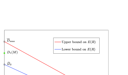
Figure 1: Lower and upper bounds on the optimal reliability function $E(R)$.

Before we proceed with the upper and lower bounds on the maximum achievable information acquisition rate and the optimal reliability function, we refer the reader to Table 1 for the list of notation introduced in Section 4. Also recall that $D_{1}(M)$ and $D_{2}(M)$ denote, respectively, the harmonic mean of $\{D_{\bolds{\mu}_{i}}(M)\}_{i\in\Omega_{M}}$ and $\{D_{\bolds{\eta}_{i}}(M)\}_{i\in\Omega_{M}}$.

Corollary 5.

For any given fixed $M$ (rate $R=0$), no policy can achieve reliability higher than $D_{1}(M)$. Also, no policy can achieve positive reliability $E>0$ at rates higher than $\overline{I}_{\max}$. Furthermore,

$$E(R)\leq\overline{D}_{\max}\biggl{(}1-\frac{R}{\overline{I}_{\max}}\biggr{)},\qquad R\in(0,\overline{I}_{\max}).$$ (19)

Remark 4.

Corollary 5 establishes an upper bound, $\overline{I}_{\max}$, on the maximum achievable information acquisition rate. As shown in the supplemental article Naghshvar-SuppA , Section 3.3, this result can be strengthened to show that no policy can achieve diminishing error probability at rates higher than $\overline{I}_{\max}$.

Corollary 6.

For fixed $M$, hence at rate $R=0$, a policy $\pi$ can achieve the maximum reliability, that is, $E=D_{1}(M)$, if and only if it is asymptotically optimal (of order-1 or higher) in $L$. Furthermore, a policy $\pi$ can achieve a nonzero rate $R>0$ with nonzero reliability $E>0$ only if it is order optimal in ${L}$ and $M$.

Corollary 6 implies that for fixed $M$, hence at $R=0$, policies $\tilde{\pi}_{1}$ and $\pi^{*}$ achieve the optimal error exponent, while policy $\tilde{\pi}_{2}$ might or might not [depending on condition (5)]. Furthermore, Corollary 6, in effect, underlines the deficiency of characterizing the solution to Problems (P) in terms of $L$ in isolation from $M$, hence, Chernoff’s notion of asymptotic optimality (solely in $L$). In particular, an order optimal policy can achieve nonzero rate and reliability simultaneously, an improvement over $\tilde{\pi}_{1}$ (and all extensions of Chernoff59 ).

Corollary 7.

Policy $\tilde{\pi}_{2}$ achieves rate $R\in[0,\underline{I}_{2}]$ with reliability $E$ if

$$E\leq\underline{D}_{2}\biggl{(}1-\frac{R}{\underline{I}_{2}}\biggr{)}.$$ (20)

Figure 1 summarizes the results above. The upper bound on the reliability function is shown in red. Policy $\tilde{\pi}_{1}$ achieves the optimal reliability $D_{1}(M)$ for fixed $M$ (at $R=0$) with no provable guarantee for $R>0$ (this point is shown in green), while policy $\tilde{\pi}_{2}$ ensures an exponentially decaying error probability (the error exponent is shown in blue) for $R\in[0,\underline{I}_{2})$.

Remark 5.

It can be shown that any optimal policy $\pi^{*}$ for Problem (P) also achieves any rate $R\in[0,\underline{I}_{2}]$ with reliability $E$ satisfying (20) for Problem (P^′).

The proofs of all the results in this section are provided in the supplemental article Naghshvar-SuppA , Section 3, and are based on the fact that Problem (P) can be viewed as a Lagrangian relaxation of Problem (P^′). It is somewhat intuitive that as ${L}\to\infty$ the solution of Problem (P) is closely related to that of Problem (P^′) when $\varepsilon\to 0$. The following lemma makes this intuition precise.

Lemma 2.

Let $\mathbb{E}[\tau^{*}_{\varepsilon}]$ denote the minimum expected number of samples required to achieve $\operatorname{Pe}\leq\varepsilon$. We have

$$\mathbb{E}\bigl{[}\tau^{*}_{\varepsilon}\bigr{]}\geq(1-\varepsilon{L})\bigl{(}V^{*}\bigl{(}\bolds{\rho}(0)\bigr{)}-1\bigr{)},$$ (21)

where $V^{*}(\bolds{\rho}(0))$ is the optimal solution to Problem (P) for prior belief $\bolds{\rho}(0)$ and penalty of wrong declaration ${L}$.

Given the above connection, Corollary 5 follows readily from the lower bounds obtained in Proposition 1 and Theorem 2 (in particular, its Corollary 3), and Corollaries 6 and 7 follow from the upper bounds given by Proposition 2 and Theorem 3.

6 Examples

In this section we consider important special cases of the active hypothesis testing to provide some intuition about the conditions of Corollaries 2 and 4, and, in particular, establish the order-2 asymptotic optimality of $\tilde{\pi}_{2}$ for a fixed value of $M$ and rate–reliability optimality of policy $\tilde{\pi}_{2}$.

6.1 Binary hypothesis testing

Consider Problem (P) for $M=2$. In this setting, policies $\tilde{\pi}_{1}$ and $\tilde{\pi}_{2}$ are equivalent and by Corollary 2, both policies are asymptotically optimal of order-1 in ${L}$. Asymptotic optimality of order-2 of $\tilde{\pi}_{1}$ and $\tilde{\pi}_{2}$ is also verified from Corollary 2 since equality (5) holds trivially for $M=2$. Furthermore, we obtain

$$V^{*}(\bolds{\rho})=\rho_{1}\frac{\log{L}-\log(\rho_{1}/\rho_{2})}{\max_{a\in\mathcal{A}_{M}}D(q^{a}_{1}\|q^{a}_{2})}+\rho_{2}\frac{\log{L}-\log(\rho_{2}/\rho_{1})}{\max_{a\in\mathcal{A}_{M}}D(q^{a}_{2}\|q^{a}_{1})}+O(1).$$

The problem of reliability (error exponent) associated with passive binary hypothesis testing with fixed-length (nonsequential) as well as variable-length (sequential) sample size has been studied by Blahut74 , Csiszar04 , Haroutunian07 . The generalization to channel coding with feedback with two messages was addressed in Berlekamp64 , Nakiboglu12 , Berlin09 . Recently, the authors in Hayashi09 and PolyanskiyITA2011 have generalized this problem for fixed-length and variable-length sample size, respectively, to the active binary hypothesis testing in the non-Bayesian context, and identified the error exponent corresponding to both error types. Our work provides nonasymptotic bounds as well as an asymptotic optimal solution in a total cost and Bayesian sense, and is consistent with the findings in PolyanskiyITA2011 .

6.2 Noisy dynamic search

Consider the problem of sequentially searching for a single target in $M$ locations where the goal is to find the target quickly and accurately. In each step, the player can inspect an allowable combination of the locations, and the outcome of the inspection is noisy. This problem is closely related to the problems of fault detection, whereabouts search and group testing. In fault detection, the objective is to determine the faulty component in a system known to have one failed component Nachlas90 , Castanon95 . In whereabouts search, the goal is to find an object which is hidden in one of $M$ boxes, where it is usually assumed that there is no false alarm, that is, the outcome of inspecting box $i$ is always $0$ if no object is present, and is a Bernoulli random variable with a known parameter otherwise Tognetti68 , Kadane71 . In group testing, the goal is to locate the nonzero element of a vector in $\mathbb{R}^{M}$ with a possible noisy linear measurement of the vector Sejdinovic10 , Chan11 . One possible search strategy for these problems is the maximum likelihood policy. In the case of fault detection/whereabouts search, this policy is equivalent to one that inspects a segment with the highest probability of having the faulty component/hidden object, while in the case of group testing, it is equivalent to measuring the most likely nonzero element of the vector. However, as the number of segments or the dimension of vectors, $M$, increases, the scheme becomes impractical. In such a case, it is more intuitive to initially follow a noisy binary search Horstein63 , Burnashev74 , Nowak11IT and narrow down the search to single segments only after we have collected sufficient information supporting the presence of the target in those segments Posner63 , Stone75 .

In this section, we first consider the problem of a noisy dynamic search with size-dependent Bernoulli noise whose special cases have been independently studied in Horstein63 , Tognetti68 , Kadane71 , Burnashev74 , Nachlas90 , Sejdinovic10 , Chan11 , Nowak11IT . Remark 6 at the end of this section discusses a generalization for the symmetric noise model of Castanon95 .

Let $a\subset\Omega_{M}$ be a subset of locations that can be simultaneously inspected, referred to as the inspection region hereafter, and let $\mathcal{A}_{M}=2^{\Omega_{M}}$ be the collection of all allowable inspection regions. We assume that the outcome of an inspection depends on the size of the inspection region. More precisely, the outcome of inspecting region $a$, where $|a|=n$, is a random variable with Bernoulli distribution:

$$q^{a}_{i}=\cases{\mathcal{B}(1-p_{n}),&\quad if $i\in a$ and $|a|=n$\vspace*{2pt}\cr\mathcal{B}(p_{n}),&\quad if $i\notin a$ and $|a|=n$}\qquad\forall i\in\Omega_{M},\forall a\in\mathcal{A}_{M},$$

where $p_{1}>0$ and for all $n$, $p_{n}\leq p_{n+1}$ and $p_{n}\leq p$ for some $p<0.5$.

Lemma 3.

Consider the problem of a noisy dynamic search with size-dependent Bernoulli noise explained above. We have

$$\min_{j\neq i}\max_{a\in\mathcal{A}_{M}}D\bigl{(}q^{a}_{i}\|q^{a}_{j}\bigr{)}={D}_{\bolds{\eta}_{i}}(M)=(1-2p_{1})\log\frac{1-p_{1}}{p_{1}}\qquad\forall i\in\Omega_{M},$$ (24)

$$\underline{D}_{2}=\overline{D}_{\max}=(1-2p_{1})\log\frac{1-p_{1}}{p_{1}},$$

$$0<1-\sup_{n}H\bigl{(}[p_{n},1-p_{n}]\bigr{)}\leq\underline{I}_{2}\leq\overline{I}_{\max}\leq 1-H\bigl{(}[p_{1},1-p_{1}]\bigr{)}.$$

The proof is provided in the supplemental article Naghshvar-SuppA , Section 4.

Lemma 3, together with Corollaries 2 and 4, implies that $\tilde{\pi}_{2}$ attains asymptotic optimality of order-2 in ${L}$, and order optimality in ${L}$ and $M$. Furthermore, for the special case of size-independent Bernoulli noise where $0<p_{1}=p_{2}=\cdots=p<0.5$, policy $\tilde{\pi}_{2}$ attains asymptotic optimality of order-1 in ${L}$ and $M$.

The active hypothesis testing scheme proposed by Chernoff Chernoff59 as well as its variants Bessler60 , Blot73 , when specialized to a noisy dynamic search with size-independent Bernoulli noise, simplifies to one that inspects, at each instant, a location with the highest probability of having the target. This scheme, which was also studied in Castanon95 in a finite horizon context, has an information acquisition rate that is restricted to zero, while at zero rate, it achieves asymptotic optimality and maximum error exponent $\overline{D}_{\max}=(1-2p)\log\frac{1-p}{p}$. In contrast, in Horstein63 , Burnashev74 , a noisy binary search was proposed in which the locations are partitioned along the median of the posterior and, in effect, are inspected along a generalized binary tree. It was shown in Horstein63 , Burnashev74 that the proposed policy can achieve any rate $R<1-H([p,1-p])$ with reliability $E(R)=1-H([p,1-p])-R$. In other words, the proposed policy in Horstein63 , Burnashev74 is asymptotically optimal in $M$ (since $1-H([p,1-p])=\overline{I}_{\max}$) but only order optimal in ${L}$ (since $0<1-H([p,1-p])<(1-2p)\log\frac{1-p}{p}=\overline{D}_{\max}$). Lemma 3 shows that, in the case of size-independent Bernoulli noise, our proposed policy $\tilde{\pi}_{2}$ combines the best of the above two approaches: in its first phase, by randomly selecting actions from $\mathcal{A}_{M}$, it ensures the maximum acquisition rate obtained by the noisy binary search of Horstein63 , Burnashev74 , while its second phase coincides with the schemes in Chernoff59 , Bessler60 , Blot73 , ensuring the maximum feasible error exponent.

Remark 6.

Lemma 3 can be extended beyond the Bernoulli noise model so long as the observation kernels

$$q^{a}_{i}(\cdot)=\cases{f_{n}(\cdot),&\quad if $i\in a$ and $|a|=n$\vspace*{2pt}\cr\bar{f}_{n}(\cdot),&\quad if $i\notin a$ and $|a|=n$}\qquad\forall i\in\Omega_{M},\forall a\in\mathcal{A}_{M},$$

satisfy the following conditions:

$$f_{n}(z)=\bar{f}_{n}(b-z)\qquad\forall z\in\mathcal{Z}\mbox{ for some }b\in\mathbb{R},$$ (26)

$$D(f_{n}\|\alpha f_{n}+\bar{\alpha}\bar{f}_{n})\geq D(f_{n+1}\|\alpha f_{n+1}+\bar{\alpha}\bar{f}_{n+1})\qquad\forall\alpha\in[0,1],\bar{\alpha}=1-\alpha,$$

$$\sup_{n}\sup_{z\in\mathcal{Z}}f_{n}(z)/\bar{f}_{n}(z)<\infty.$$ (27)

In particular, under these conditions

$$\min_{j\neq i}\max_{a\in\mathcal{A}_{M}}D\bigl{(}q^{a}_{i}\|q^{a}_{j}\bigr{)}={D}_{\bolds{\eta}_{i}}(M)=D(f_{1}\|\bar{f}_{1})\qquad\forall i\in\Omega_{M},$$ (28)

$$\underline{D}_{2}=\overline{D}_{\max}=D(f_{1}\|\bar{f}_{1}),$$ (29)

$$\inf_{n}D\biggl{(}f_{n}\bigg{\|}\frac{1}{2}f_{n}+\frac{1}{2}\bar{f}_{n}\biggr{)}\leq\underline{I}_{2}\leq\overline{I}_{\max}\leq D\biggl{(}f_{1}\bigg{\|}\frac{1}{2}f_{1}+\frac{1}{2}\bar{f}_{1}\biggr{)}.$$ (30)

Condition (26) implies that given a fixed inspection area, the collected samples provide identical information regarding the presence of the target or its absence. Condition (26) implies that the samples become less informative as the size of the inspection region increases. Conditions (26) and (26) are natural, while condition (27) is a technical one to ensure that Assumptions 2 and 3 hold (we address weakening these assumptions in Section 7).

7 Discussions

In this section we provide a discussion on the technical assumptions of the paper. In particular, we discuss the necessity of our Assumptions 1 and 2, and compare them with the common assumptions in the literature. In contrast to Assumption 1 which is shown to be necessary for the problem of active hypothesis testing to have a meaningful solution, Assumption 2 can be relaxed to more general assumptions without affecting the asymptotic results of the paper.

7.1 Assumption 1

We first discuss the necessity of Assumption 1. If Assumption 1 does not hold, then there exist two hypotheses $i,j\in\Omega_{M}$, $i\neq j$ such that for all $a\in\mathcal{A}_{M}$, $D(q^{a}_{i}\|q^{a}_{j})=0$. In other words, $q^{a}_{i}(\cdot)=q^{a}_{j}(\cdot)$ for all $a\in\mathcal{A}_{M}$, and, hence, the decision maker is not capable of distinguishing these two hypotheses. In this sense, Assumption 1 is necessary for Problem (P) to be meaningful.

Next we compare Assumption 1 to its counterpart in Chernoff59 :

Assumption 1^′.

$D(q_{i}^{a}\|q_{j}^{a})>0$, $\forall i,j\in\Omega_{M}$, $i\neq j$, $\forall a\in\mathcal{A}_{M}$.

This assumption assures consistency (see Lemma 1 in Chernoff59 ), that is,$\arg\max_{i\in\Omega_{M}}\rho_{i}(t)$ converges exponentially fast to the true hypothesis regardless of the way the sensing actions are selected. However, this assumption is very restrictive and does not hold in many problems of interest such as channel coding with feedback Burnashev76 and noisy dynamic search (e.g., one cannot discriminate between locations 1 and 2 by inspecting location 3). It was remarked in Chernoff59 , Section 7, that the above restrictive assumption can be relaxed if the proposed scheme is modified to take a (possibly randomized) action capable of discriminating between all hypotheses pairs infinitely often (e.g., at any time $t$ when $t$ is a perfect square). In this paper, however, we took a different approach and constructed policy $\tilde{\pi}_{1}$, a simple two-phase modification of Chernoff’s original scheme in which testing for the maximum likely hypothesis is delayed and contingent on obtaining a certain level of confidence.

7.2 Assumption 2

We first discuss the necessity of Assumption 2. For observation kernels with bounded support, Assumption 2 is a necessary condition to ensure that the observation kernels are absolutely continuous with respect to each other and, hence, no observation is noise free. Although this assumption might hold in many settings such as the problem of a noisy dynamic search with Bernoulli noise explained in Section 6.2, it does not hold in general for observation kernels with unbounded support such as Gaussian distribution. Next we replace Assumption 2 by more general assumptions on the observation kernels and discuss the consequences.

To the best of our knowledge, Assumption 2^′ below, given first by Chernoff59 , is the weakest condition in the literature of hypothesis testing and sequential analysis, and is often interpreted to an assumption which limits the excess over the boundary at the stopping time Lorden70 .

Assumption 2^′.

There exists $\xi_{M}<\infty$ such that

$$\max_{i,j\in\Omega_{M}}\max_{a\in\mathcal{A}_{M}}\int_{\mathcal{Z}}q_{i}^{a}(z)\biggl{|}\log\frac{q_{i}^{a}(z)}{q_{j}^{a}(z)}\biggr{|}^{2}\,dz\leq\xi_{M}.$$

Proposition 1 remains valid even if Assumption 2 is replaced with Assumption 2^′ (with the only change that $\xi_{M}^{2}$ is replaced with $\xi_{M}$ in the bound). The proof of Proposition 2 relies on Chernoff’s approach Chernoff59 , and the asymptotic behavior of the bound remains intact if Assumption 2 is replaced with Assumption 2^′. However, as shown in the proof of this proposition in the supplemental article Naghshvar-SuppA , Section 5, Assumption 2 allows us to give a precise nonasymptotic characterization of the bound by applying the method of bounded differences and, in particular, McDiarmid’s inequality McDiarmid89 .

Next we consider the consequence of weakening Assumption 2 on Theorems 2 and 3, hence on the performance of policy $\tilde{\pi}_{2}$. To do so, we consider an even weaker assumption than Assumption 2^′ as given below:

Assumption 2^′′.

There exist $\xi_{M}<\infty$ and $\gamma>0$ such that

$$\max_{i,j\in\Omega_{M}}\max_{a\in\mathcal{A}_{M}}\int_{\mathcal{Z}}q_{i}^{a}(z)\biggl{|}\log\frac{q_{i}^{a}(z)}{q_{j}^{a}(z)}\biggr{|}^{1+\gamma}\,dz\leq\xi_{M}.$$

Define function $\psi_{M}\dvtx\mathbb{R}_{+}\to\mathbb{R}_{+}$ as follows:

$$\psi_{M}(b):=\max_{i,j\in\Omega_{M}}\max_{a\in\mathcal{A}_{M}}\int_{\mathcal{Z}}q_{i}^{a}(z)\biggl{[}\log\frac{q_{i}^{a}(z)}{q_{j}^{a}(z)}\biggr{]}_{b}\,dz,$$

where $[g]_{b}=g{\mathbf{1}}_{\{g>b\}}$. Note that $\psi_{M}(b)$ is in general nonincreasing in $b$, and if Assumption 2^′′ holds, $\psi_{M}(b)\leq b^{-\gamma}\xi_{M}$. Under the weaker Assumption 2^′′ (and naturally Assumption 2^′), Theorems 2 and 3 can be replaced by the following:

Proposition 3.

Under Assumptions 1 and 2^′′ and for ${L}>\frac{\log M}{I_{\max}(M)}$, $\bolds{\rho}\in\mathbb{P}_{{L}}(\Omega_{M})$, $\delta\in(0,0.5]$, and $b>0$,

$$V^{*}(\bolds{\rho})\geq\underline{V_{3}}(\bolds{\rho}) := \frac{1}{1+\psi_{M}(b)/D_{\max}(M)}$$

$${}\times\biggl{[}\frac{H(\bolds{\rho})-H([\delta,1-\delta])-{\delta}\log(M-1)}{I_{\max}(M)}$$

$$\hskip 17.0pt{}+\frac{\log((1-{L}^{-1})/L^{-1})-\log((1-\delta)/\delta)-b}{D_{\max}(M)}$$

$$\hskip 105.0pt{}\times\mathbf{1}_{\{\max_{i\in\Omega_{M}}\rho_{i}\leq 1-\delta\}}-K^{\prime}_{3}\biggr{]}^{+},$$

where $K^{\prime}_{3}$ is a positive constant independent of $\delta$ and ${L}$. In addition, if Assumption 3 also holds, then $K^{\prime}_{3}$ can be selected independent of $M$ as well.

The proof is provided in the supplemental article Naghshvar-SuppA , Section 8.1.

Proposition 4.

Under Assumptions 1 and 2^′′, and for ${L}>1$ and $\bolds{\rho}\in\mathbb{P}_{{L}}(\Omega_{M})$, $\exists b^{\prime}\in(0,\infty)$ such that for all $b\geq b^{\prime}$, $0\leq\frac{(1+(\log e)/b)2^{-b}\psi_{M}(b)}{I_{2}(M)-\psi_{M}(b)}<1$, and

$$V^{*}(\bolds{\rho}) \leq \overline{V}_{3}(\bolds{\rho})$$

$$:= \biggl{(}1-\frac{(1+(\log e)/b)2^{-b}\psi_{M}(b)}{I_{2}(M)-\psi_{M}(b)}\biggr{)}^{-1}$$

$${}\times\Biggl{(}\frac{H(\bolds{\rho})+\log(\tilde{\rho}/(1-\tilde{\rho}))+b+\log e}{I_{2}(M)-\psi_{M}(b)}+\sum_{i=1}^{M}\rho_{i}\frac{\log{L}}{D_{\bolds{\eta}_{i}}(M)-\psi_{M}(b)}\Biggr{)}$$

$${}+1.$$

The proof is provided in the supplemental article Naghshvar-SuppA , Section 8.2.

As we discussed, $\psi_{M}(b)\leq b^{-\gamma}\xi_{M}$ under Assumption 2^′′. Furthermore, if Assumption 3 holds, then $\sup_{M}\psi_{M}(b)\leq b^{-\gamma}\xi$. In other words, we can select $b$ as a function of ${L}$ and $M$ (e.g., $b=\log\log{L}M$) such that $\underline{V_{3}}$ and $\overline{V}_{3}$ have the same dominating terms (in ${L}$ and $M$) as $\underline{V_{2}}$ and $\overline{V}_{2}$, respectively.

In summary, the asymptotic results of the paper presented in Section 5 hold under the weaker Assumptions 2^′ and 2^′′ replacing Assumption 2 (with the only exception that the asymptotic optimality of order-2 of policy $\tilde{\pi}_{2}$ established in Corollary 2 is degraded to asymptotic optimality of order-1). Our choice to present the work under Assumption 2, however, significantly simplifies the presentation and also enables a precise nonasymptotic characterization of the lower and upper bounds.

8 Conclusions and future work

In this paper we considered the problem of active sequential $M$-ary hypothesis testing. Using a DP formulation, we characterized the optimal value function $V^{*}$. Three lower bounds (complementary for various values of the parameters of the problem) were obtained for the optimal value function $V^{*}$. We also proposed two heuristic policies whose performance analysis resulted in two upper bounds for $V^{*}$. Subsequently, we discussed important consequences of the bounds and established order and asymptotic optimality of the proposed policies under different scenarios. An important problem which remains is further improvement of the performance bounds.

In this paper we focused on sequential policies, that is, policies whose sample size is not known initially and is dependent on the observation outcomes. There exist other types of policies in the literature. For example, nonsequential policies take a fixed number of samples (independent of observation outcomes) and make the final decision afterward, while multi-stage policies (introduced in Lorden83 , Bartroff07 ) can take a retire–declare action only at the end of each stage, and stages are not necessarily of the same size. Comparing the performance of sequential, nonsequential and multi-stage policies in the context of active hypothesis testing is an area of future work.

In this paper we assumed that all sensing actions incur one unit of cost (each action can be executed in one unit of time). It is also of interest to consider the scenario where there is a cost associated with each action which, for example, characterizes the amount of energy or time required to perform that action; and the goal is to find the true hypothesis subject to a cost criterion. Such generalization has been studied for the problem of variable-length coding with feedback in Nakiboglu08 .

Appendix: Proof of Theorems 1–3

.1 Proof of Theorem 1

Let ${\Gamma}$ be the set of all mappings $\gamma\dvtx\Omega_{M}\to\Omega_{M}$ such that $\gamma(i)\neq i$ for $i\in\Omega_{M}$. Now associated with any $\gamma\in{\Gamma}$, define

$$\underline{V_{1}}^{\gamma}(\bolds{\rho})=\Biggl{[}\sum_{i=1}^{M}\rho_{i}\frac{\log((1-L^{-1})/L^{-1})-\log(\rho_{i}/\rho_{\gamma(i)})}{\max_{\hat{a}\in\mathcal{A}_{M}}D(q^{\hat{a}}_{i}\|q^{\hat{a}}_{\gamma(i)})}-K^{\prime}_{1}\Biggr{]}^{+}.$$ (31)

Next we use Lemma 1 to show that $V^{*}\geq\underline{V_{1}}^{\gamma}$ for all $\gamma\in\Gamma$. In particular, we show that for all $\gamma\in\Gamma$ and all $\bolds{\rho}\in\mathbb{P}(\Omega_{M})$, $\underline{V_{1}}^{\gamma}(\bolds{\rho})\leq\min\{1+\min_{a\in\mathcal{A}_{M}}(\mathbb{T}^{a}\underline{V_{1}}^{\gamma})(\bolds{\rho}),\min_{j\in\Omega_{M}}(1-\rho_{j}){L}\}$. For any $\bolds{\rho}$ such that $\underline{V_{1}}^{\gamma}(\bolds{\rho})=0$, the inequality holds trivially. For $\underline{V_{1}}^{\gamma}(\bolds{\rho})>0$ and for any action $a\in\mathcal{A}_{M}$, we have

$$\bigl{(}\mathbb{T}^{a}\underline{V_{1}}^{\gamma}\bigr{)}(\bolds{\rho})$$

$$\qquad\geq\sum_{i=1}^{M}\int\rho_{i}q^{a}_{i}(z)\frac{\log((1-L^{-1})/L^{-1})-\log(\rho_{i}q^{a}_{i}(z)/(\rho_{\gamma(i)}q^{a}_{\gamma(i)}(z)))}{\max_{\hat{a}\in\mathcal{A}_{M}}D(q^{\hat{a}}_{i}\|q^{\hat{a}}_{\gamma(i)})}\,dz$$

$$\quad\qquad{}-K^{\prime}_{1}$$

$$\qquad=\underline{V_{1}}^{\gamma}(\bolds{\rho})-\sum_{i=1}^{M}\rho_{i}\frac{D(q^{a}_{i}\|q^{a}_{\gamma(i)})}{\max_{\hat{a}\in\mathcal{A}_{M}}D(q^{\hat{a}}_{i}\|q^{\hat{a}}_{\gamma(i)})}$$

$$\qquad\geq\underline{V_{1}}^{\gamma}(\bolds{\rho})-1.$$

Claim 1 ((In Section 9.1 of the supplemental article Naghshvar-SuppA )).

Constant $K^{\prime}_{1}$ can be selected independent of ${L}$ such that $\underline{V_{1}}^{\gamma}(\bolds{\rho})\leq\min_{j\in\Omega_{M}}(1-\rho_{j}){L}$ is satisfied for all $\gamma\in\Gamma$.

Using Claim 1 and letting $\underline{V_{1}}(\cdot)=\max_{\gamma\in\Gamma}\underline{V_{1}}^{\gamma}(\cdot)$, we have the assertion of the theorem.

.2 Proof of Theorem 2

We first show that for all $\bolds{\rho}\in\mathbb{P}(\Omega_{M})$,

$$V^{*}(\bolds{\rho}) \geq \biggl{[}\frac{H(\bolds{\rho})-H([\alpha({L},M),1-\alpha({L},M)])-\alpha({L},M)\log(M-1)}{I_{\max}(M)}$$

$$\hskip 218.0pt{}+\alpha({L},M){L}\biggr{]}^{+}\!.$$

Note that the right-hand side of (LABEL:LBG) can be written as

$$G(\bolds{\rho}):=\biggl{[}\frac{H(\bolds{\rho})-H(\bolds{\nu})}{I_{\max}(M)}+\alpha({L},M){L}\biggr{]}^{+},$$ (33)

where

$$\bolds{\nu}=\biggl{[}\frac{\alpha({L},M)}{M-1},\ldots,\frac{\alpha({L},M)}{M-1},1-\alpha({L},M)\biggr{]}.$$ (34)

Next we show that $G(\bolds{\rho})\leq\min\{1+\min_{a\in\mathcal{A}_{M}}(\mathbb{T}^{a}G)(\bolds{\rho}),\min_{j\in\Omega_{M}}(1-\rho_{j}){L}\}$ for all $\bolds{\rho}\in\mathbb{P}(\Omega_{M})$. For any $\bolds{\rho}$ such that $G(\bolds{\rho})=0$, the inequality holds trivially. For $G(\bolds{\rho})>0$ and for any action $a\in\mathcal{A}_{M}$, we have

$$\bigl{(}\mathbb{T}^{a}G\bigr{)}(\bolds{\rho}) = \frac{\int H(\bolds{\Phi}^{a}(\bolds{\rho},z))q^{a}_{\bolds{\rho}}(z)\,dz-H(\bolds{\nu})}{I_{\max}(M)}+\alpha({L},M){L}$$

$$= \frac{H(\bolds{\rho})-I(\bolds{\rho};q^{a}_{\bolds{\rho}})-H(\bolds{\nu})}{I_{\max}(M)}+\alpha({L},M){L}$$

$$= G(\bolds{\rho})-\frac{I(\bolds{\rho};q^{a}_{\bolds{\rho}})}{I_{\max}(M)}$$

$$\geq G(\bolds{\rho})-1,$$

where the last inequality follows from the fact that

$$I\bigl{(}\bolds{\rho};q^{a}_{\bolds{\rho}}\bigr{)}\leq\max_{\hat{a}\in\mathcal{A}_{M}}\max_{\hat{\bolds{\rho}}\in\mathbb{P}(\Omega_{M})}I\bigl{(}\hat{\bolds{\rho}};q^{\hat{a}}_{\hat{\bolds{\rho}}}\bigr{)}=I_{\max}(M).$$

Therefore,

$$G(\bolds{\rho})\leq 1+\min_{a\in\mathcal{A}_{M}}\bigl{(}\mathbb{T}^{a}G\bigr{)}(\bolds{\rho}).$$

What remains is to show that $G(\bolds{\rho})\leq\min_{j\in\Omega_{M}}(1-\rho_{j}){L}$. Rewriting $G$ as

$$G(\bolds{\rho}) = \biggl{[}\frac{\sum_{i=1}^{M-1}\rho_{i}\log(1/\rho_{i})+(1-\sum_{i=1}^{M-1}\rho_{i})\log(1/(1-\sum_{i=1}^{M-1}\rho_{i}))-H(\bolds{\nu})}{I_{\max}(M)}$$

$$\hskip 251.0pt{}+\alpha({L},M){L}\biggr{]}^{+}\!,$$

we can compute the gradient at $\bolds{\nu}$. For all $i=1,2,\ldots,M-1$,

$$\frac{\partial G}{\partial\rho_{i}}(\bolds{\nu}) = \biggl{(}\log\frac{1}{\rho_{i}}-\log e-\log\frac{1}{1-\sum_{i=1}^{M-1}\rho_{i}}+\log e\biggr{)}\Big{/}I_{\max}(M)\bigg{|}_{\bolds{\rho}=\bolds{\nu}}$$

$$= \biggl{(}\log\frac{\rho_{M}}{\rho_{i}}\biggr{)}\Big{/}I_{\max}(M)\Big{|}_{\bolds{\rho}=\bolds{\nu}}=\biggl{(}\log\frac{1-\alpha({L},M)}{\alpha({L},M)/(M-1)}\biggr{)}\Big{/}I_{\max}(M)={L}.$$

Furthermore, $G(\bolds{\nu})=\alpha({L},M){L}=(1-\nu_{M}){L}$. Without loss of generality and since both functions $G(\bolds{\rho})$ and $\min_{j\in\Omega_{M}}(1-\rho_{j}){L}$ are symmetric, let us focus on $\mathbb{P}_{M}(\Omega_{M}):=\{\bolds{\rho}\in\mathbb{P}(\Omega_{M})\dvtx\rho_{M}\geq\rho_{i},\ \forall i\in\Omega_{M}-\{M\}\}$. In this case, $\min_{j\in\Omega_{M}}(1-\rho_{j}){L}=(1-\rho_{M}){L}=\sum_{i=1}^{M-1}\rho_{i}{L}$ and, hence, $\min_{j\in\Omega_{M}}(1-\rho_{j}){L}$ is the tangent hyperplane to $G(\bolds{\rho})$ at $\bolds{\nu}$. This along with concavity of function $G$ implies $G(\bolds{\rho})\leq\min_{j\in\Omega_{M}}(1-\rho_{j}){L}$. Using Lemma 1, we have the assertion of the theorem.

Next we need to show that

$$V^{*}(\bolds{\rho})\geq\underline{V_{2}}(\bolds{\rho}) = \biggl{[}\frac{H(\bolds{\rho})-H([\delta,1-\delta])-{\delta}\log(M-1)}{I_{\max}(M)}$$

$$\hskip 4.0pt{}+\frac{\log((1-L^{-1})/L^{-1})-\log((1-\delta)/\delta)-\xi_{M}}{D_{\max}(M)}$$

$$\hskip 99.0pt{}\times{\mathbf{1}}_{\{\max_{i\in\Omega_{M}}\rho_{i}\leq 1-\delta\}}-K^{\prime}_{2}\biggr{]}^{+}.$$

We show this in two steps. First we consider the following function:

$$J^{\prime}(\bolds{\rho}) := \Biggl{[}\sum_{i=1}^{M}\rho_{i}\frac{\log((1-L^{-1})/L^{-1})-\log(\rho_{i}/(1-\rho_{i}))}{D_{\max}(M)}-K^{\prime}_{2}\Biggr{]}^{+}.$$ (37)

We use Jensen’s inequality to show that

$$J^{\prime}(\bolds{\rho})\leq 1+\min_{a\in\mathcal{A}_{M}}\bigl{(}\mathbb{T}^{a}J^{\prime}\bigr{)}(\bolds{\rho})\qquad\forall\bolds{\rho}\in\mathbb{P}(\Omega_{M}).$$ (38)

For any $\bolds{\rho}$ such that $J^{\prime}(\bolds{\rho})=0$, inequality (38) holds trivially. For any $\bolds{\rho}$ such that $J^{\prime}(\bolds{\rho})>0$ and for any $a\in\mathcal{A}_{M}$, we have

$$\bigl{(}\mathbb{T}^{a}J^{\prime}\bigr{)}(\bolds{\rho})$$

$$\qquad\geq\sum_{i=1}^{M}\int\rho_{i}q^{a}_{i}(z)\frac{\log((1-L^{-1})/L^{-1})-\log(\rho_{i}q^{a}_{i}(z)/\sum_{j\neq i}\rho_{j}q^{a}_{j}(z))}{D_{\max}(M)}\,dz$$

$$\quad\qquad{}-K^{\prime}_{2}$$

$$\qquad=J^{\prime}(\bolds{\rho})-\sum_{i=1}^{M}\rho_{i}\frac{\int q^{a}_{i}(z)\log(q^{a}_{i}(z)/\sum_{j\neq i}(\rho_{j}/(1-\rho_{i}))q^{a}_{j}(z))\,dz}{D_{\max}(M)}$$

$$\qquad\geq J^{\prime}(\bolds{\rho})-\sum_{i=1}^{M}\rho_{i}\frac{\sum_{j\neq i}(\rho_{j}/(1-\rho_{i}))D(q^{a}_{i}\|q^{a}_{j})}{D_{\max}(M)}$$

$$\qquad\geq J^{\prime}(\bolds{\rho})-1.$$

Next we define $J(\bolds{\rho})=\max\{J^{\prime}(\bolds{\rho}),J^{\prime\prime}(\bolds{\rho})\}$, where $J^{\prime\prime}(\bolds{\rho})$ is the right-hand side of (.2), that is,

$$J^{\prime\prime}(\bolds{\rho}) = \biggl{[}\frac{H(\bolds{\rho})-H([\delta,1-\delta])-{\delta}\log(M-1)}{I_{\max}(M)}$$

$$\hskip 4.0pt{}+\frac{\log((1-L^{-1})/L^{-1})-\log((1-\delta)/\delta)-\xi_{M}}{D_{\max}(M)}$$

$$\hskip 100.0pt{}\times\mathbf{1}_{\{\max_{i\in\Omega_{M}}\rho_{i}\leq 1-\delta\}}-K^{\prime}_{2}\biggr{]}^{+}.$$

• Case 1: For all $\bolds{\rho}$ such that $J(\bolds{\rho})=0$ or $J(\bolds{\rho})=J^{\prime}(\bolds{\rho})$, it is trivial from (38) that

  $$J(\bolds{\rho})=J^{\prime}(\bolds{\rho})\leq 1+\min_{a\in\mathcal{A}_{M}}\bigl{(}\mathbb{T}^{a}J^{\prime}\bigr{)}(\bolds{\rho})\leq 1+\min_{a\in\mathcal{A}_{M}}\bigl{(}\mathbb{T}^{a}J\bigr{)}(\bolds{\rho}).$$ (40)

• Case 2: For all $\bolds{\rho}$ such that $J(\bolds{\rho})=J^{\prime\prime}(\bolds{\rho})>0$, and for any action $a\in\mathcal{A}_{M}$, we have

  $$\bigl{(}\mathbb{T}^{a}J\bigr{)}(\bolds{\rho}) = \int J\bigl{(}\bolds{\Phi}^{a}(\bolds{\rho},z)\bigr{)}q^{a}_{\bolds{\rho}}(z)\,dz$$

  $$\stackrel{{\scriptstyle(a)}}{{\geq}} \frac{\int H(\bolds{\Phi}^{a}(\bolds{\rho},z))q^{a}_{\bolds{\rho}}(z)\,dz-H([\delta,1-\delta])-{\delta}\log(M-1)}{I_{\max}(M)}$$

  $${}+\frac{\log((1-L^{-1})/L^{-1})-\log((1-\delta)/\delta)-\xi_{M}}{D_{\max}(M)}$$

  $$\quad{}\times\mathbf{1}_{\{\max_{i\in\Omega_{M}}\rho_{i}\leq 1-\delta\}}-K^{\prime}_{2}$$

  $$= J^{\prime\prime}(\bolds{\rho})-\frac{I(\bolds{\rho};q^{a}_{\bolds{\rho}})}{I_{\max}(M)}$$

  $$\geq J^{\prime\prime}(\bolds{\rho})-1$$

  $$\stackrel{{\scriptstyle(b)}}{{=}} J(\bolds{\rho})-1,$$

  where ($a$) follows from Claim 2 below and ($b$) holds since $\bolds{\rho}$ is such that $J(\bolds{\rho})=J^{\prime\prime}(\bolds{\rho})$.

Claim 2 ((In Section 9.2 of the supplemental article Naghshvar-SuppA )).

Let $\bolds{\rho}$ be such that $J(\bolds{\rho})=J^{\prime\prime}(\bolds{\rho})>0$. If Assumption 2 holds, then for all actions $a\in\mathcal{A}_{M}$ and observations $z\in\mathcal{Z}$,

$$J\bigl{(}\bolds{\Phi}^{a}(\bolds{\rho},z)\bigr{)} \geq \frac{H(\bolds{\Phi}^{a}(\bolds{\rho},z))-H([\delta,1-\delta])-{\delta}\log(M-1)}{I_{\max}(M)}$$

$${}+\frac{\log((1-L^{-1})/L^{-1})-\log((1-\delta)/\delta)-\xi_{M}}{D_{\max}(M)}$$

$$\quad{}\times\mathbf{1}_{\{\max_{i\in\Omega_{M}}\rho_{i}\leq 1-\delta\}}-K^{\prime}_{2}.$$

Combining (40) and (• ‣ .2), we have that

$$J(\bolds{\rho})\leq 1+\min_{a\in\mathcal{A}_{M}}\bigl{(}\mathbb{T}^{a}J\bigr{)}(\bolds{\rho}).$$ (43)

We also have the following:

Claim 3 ((In Section 9.3 of the supplemental article Naghshvar-SuppA )).

For ${L}>\frac{\log M}{I_{\max}(M)}$, constant $K^{\prime}_{2}$ can be selected independent of $\delta$ and ${L}$ such that $J(\bolds{\rho})\leq\min_{j\in\Omega_{M}}(1-\rho_{j}){L}$. Furthermore, if $\sup_{M}\xi_{M}<\infty$, then $K^{\prime}_{2}$ can be selected independent of $M$ as well.

Lemma 1, together with (43) and Claim 3, implies that $V^{*}\geq J=\break\max\{J^{\prime},J^{\prime\prime}\}\geq J^{\prime\prime}=\underline{V_{2}}$. This is a slightly stronger result than (.2).

.3 Proof of Theorem 3

Recall that $\rho_{i}(n)$ denotes the posterior belief about hypothesis $H_{i}$ after $n$ observations. Let $\tau$, $\tau_{i}$, $i\in\Omega_{M}$, be Markov stopping times defined as follows:

$$\tau := \min\Bigl{\{}n\dvtx\max_{j\in\Omega_{M}}\rho_{j}(n)\geq 1-{L}^{-1}\Bigr{\}},$$ (44)

$$\tau_{i} := \min\bigl{\{}n\dvtx\rho_{i}(n)\geq 1-{L}^{-1}\bigr{\}}.$$ (45)

From (1), the expected total cost under policy $\tilde{\pi}_{2}$ is upper bounded as

$$V_{\tilde{\pi}_{2}}(\bolds{\rho}) = \mathbb{E}_{\tilde{\pi}_{2}}\Bigl{[}\tau+\min_{j\in\Omega_{M}}\bigl{(}1-\rho_{j}(\tau)\bigr{)}{L}\Bigr{]}$$

$$\leq \mathbb{E}_{\tilde{\pi}_{2}}[\tau]+1$$

$$\leq \sum_{i=1}^{M}\rho_{i}\mathbb{E}_{\tilde{\pi}_{2}}[\tau_{i}|\theta=i]+1,$$

where $\bolds{\rho}=[\rho_{1},\rho_{2},\ldots,\rho_{M}]=[\rho_{1}(0),\rho_{2}(0),\ldots,\rho_{M}(0)]$ and the last inequality follows from the fact that $\tau\leq\tau_{i}$, $\forall i\in\Omega_{M}$. For notational simplicity, subscript $\tilde{\pi}_{2}$ is dropped for the rest of the proof.

Next we find an upper bound for $\mathbb{E}[\tau_{i}|\theta=i]$, $i\in\Omega_{M}$. Let

$$U_{n}:=\log\frac{\rho_{i}(n)}{1-\rho_{i}(n)}-\log\frac{\tilde{\rho}}{1-\tilde{\rho}}$$ (47)

and let $\mathcal{F}_{n}$ denote the history of previous actions and observations up to time $n$, that is, $\mathcal{F}_{n}:=\sigma\{\bolds{\rho}(0),A(0),Z(0),\ldots,A(n-1),Z(n-1)\}$. Under policy $\tilde{\pi}_{2}$, the sequence $\{U_{n}\}$, $n=0,1,\ldots,$ forms a submartingale with respect to the filtration $\{\mathcal{F}_{n}\}$ with the following properties: [(C3)]

If $U_{n}<0$ and $\rho_{j}(n)<\tilde{\rho}$ for all $j\in\Omega_{M}$ ($\Rightarrow P(A(n)=a)=\eta_{0a}$):

$$\mathbb{E}[U_{n+1}-U_{n}|\mathcal{F}_{n},\theta=i]$$

$$\qquad=\sum_{a\in\mathcal{A}_{M}}P\bigl{(}A(n)=a\bigr{)}\mathbb{E}\bigl{[}U_{n+1}-U_{n}|\mathcal{F}_{n},\theta=i,A(n)=a\bigr{]}$$

$$\qquad=\sum_{a\in\mathcal{A}_{M}}\eta_{0a}\mathbb{E}\bigl{[}U_{n+1}-U_{n}|\mathcal{F}_{n},\theta=i,A(n)=a\bigr{]}$$

$$\qquad=\sum_{a\in\mathcal{A}_{M}}\eta_{0a}\mathbb{E}\biggl{[}\log\frac{\rho_{i}(n)q^{a}_{i}(Z)}{\sum_{j\neq i}\rho_{j}(n)q^{a}_{j}(Z)}-\log\frac{\rho_{i}(n)}{1-\rho_{i}(n)}\bigg{|}\mathcal{F}_{n},\theta=i\biggr{]}$$

$$\qquad=\sum_{a\in\mathcal{A}_{M}}\eta_{0a}\int q^{a}_{i}(z)\log\frac{q^{a}_{i}(z)}{\sum_{j\neq i}(\rho_{j}(n)/(1-\rho_{i}(n)))q^{a}_{j}(z)}\,dz$$

$$\qquad\geq\max_{\bolds{\lambda}\in\mathbb{P}(\mathcal{A}_{M})}\ \min_{i\in\Omega_{M}}\ \min_{\hat{\bolds{\rho}}\in\mathbb{P}_{{L}}(\Omega_{M})}\sum_{a\in\mathcal{A}_{M}}\lambda_{a}D\biggl{(}q^{a}_{i}\bigg{\|}\sum_{j\neq i}\frac{{\hat{\rho}}_{j}}{1-\hat{\rho}_{i}}q^{a}_{j}\biggr{)}$$

$$\qquad=I_{\bolds{\eta}_{0}}(M).$$

If $U_{n}<0$ and $\rho_{k}(n)\geq\tilde{\rho}$ for some $k\neq i$ ($\Rightarrow P(A(n)=a)=\eta_{ka}$):

$$\mathbb{E}[U_{n+1}-U_{n}|\mathcal{F}_{n},\theta=i]$$

$$\qquad=\sum_{a\in\mathcal{A}_{M}}\eta_{ka}\mathbb{E}\bigl{[}U_{n+1}-U_{n}|\mathcal{F}_{n},\theta=i,A(n)=a\bigr{]}$$

$$\qquad=\sum_{a\in\mathcal{A}_{M}}\eta_{ka}\int q^{a}_{i}(z)\log\frac{q^{a}_{i}(z)}{\sum_{j\neq i}(\rho_{j}(n)/(1-\rho_{i}(n)))q^{a}_{j}(z)}\,dz$$

$$\qquad\geq\min_{i\in\Omega_{M}}\min_{k\neq i}\min_{\hat{\bolds{\rho}}\dvtx\hat{\rho}_{k}\geq\tilde{\rho}}\sum_{a\in\mathcal{A}_{M}}\eta_{ka}D\biggl{(}q^{a}_{i}\bigg{\|}\sum_{j\neq i}\frac{{\hat{\rho}}_{j}}{1-\hat{\rho}_{i}}q^{a}_{j}\biggr{)}$$

$$\qquad=I_{\bolds{\eta},\tilde{\rho}}(M);$$

If $U_{n}\geq 0$ ($\rho_{i}(n)\geq\tilde{\rho}\Rightarrow P(A(n)=a)=\eta_{ia}$):

$$\mathbb{E}[U_{n+1}-U_{n}|\mathcal{F}_{n},\theta=i]$$

$$\qquad=\sum_{a\in\mathcal{A}_{M}}\eta_{ia}\mathbb{E}\bigl{[}U_{n+1}-U_{n}|\mathcal{F}_{n},\theta=i,A(n)=a\bigr{]}$$

$$\qquad=\sum_{a\in\mathcal{A}_{M}}\eta_{ia}\int q^{a}_{i}(z)\log\frac{q^{a}_{i}(z)}{\sum_{j\neq i}(\rho_{j}(n)/(1-\rho_{i}(n)))q^{a}_{j}(z)}\,dz$$

$$\qquad\geq\max_{\bolds{\lambda}\in\mathbb{P}(\mathcal{A}_{M})}\min_{\hat{\bolds{\rho}}\in\mathbb{P}_{{L}}(\Omega_{M})}\sum_{a\in\mathcal{A}_{M}}\lambda_{a}D\biggl{(}q^{a}_{i}\bigg{\|}\sum_{j\neq i}\frac{{\hat{\rho}}_{j}}{1-\hat{\rho}_{i}}q^{a}_{j}\biggr{)}$$

$$\qquad=D_{\bolds{\eta}_{i}}(M);$$

$|U_{n}-U_{n-1}|\leq\max_{i,j\in\Omega_{M}}\max_{a\in\mathcal{A}_{M}}\sup_{z\in\mathcal{Z}}\log\frac{q^{a}_{i}(z)}{q^{a}_{j}(z)}\leq\xi_{M}$.

Stopping time $\tau_{i}$ defined in (45) can be rewritten as

$$\qquad\tau_{i} = \min\bigl{\{}n\dvtx\rho_{i}(n)\geq 1-{L}^{-1}\bigr{\}}$$

$$= \min\biggl{\{}n\dvtx\frac{\rho_{i}(n)}{1-\rho_{i}(n)}\geq\frac{1-{L}^{-1}}{{L}^{-1}}\biggr{\}}$$

$$= \min\biggl{\{}n\dvtx\log\frac{\rho_{i}(n)}{1-\rho_{i}(n)}-\log\frac{\tilde{\rho}}{1-\tilde{\rho}}\geq\log\frac{1-{L}^{-1}}{{L}^{-1}}-\log\frac{\tilde{\rho}}{1-\tilde{\rho}}\biggr{\}}$$

$$= \min\biggl{\{}n\dvtx U_{n}\geq\log\frac{1-{L}^{-1}}{{L}^{-1}}-\log\frac{\tilde{\rho}}{1-\tilde{\rho}}\biggr{\}}$$

$$\leq \min\{n\dvtx U_{n}\geq\log{L}\}.$$

The assertion of the theorem follows from (.3) and the following lemma.

Lemma 4.

Consider the sequence $\{U_{n}\}$, $n=0,1,\ldots$ defined in (47), and assume there exist positive constants $K_{1}\leq K_{2}\leq K_{3}$ such that

$$\mathbb{E}[U_{n+1}|\mathcal{F}_{n},\theta=i] \geq U_{n}+K_{1}\qquad\mbox{if }U_{n}<0,$$

$$\mathbb{E}[U_{n+1}|\mathcal{F}_{n},\theta=i] \geq U_{n}+K_{2}\qquad\mbox{if }U_{n}\geq 0,$$

$$|U_{n+1}-U_{n}| \leq K_{3}.$$

Consider the stopping time $\upsilon=\min\{n\dvtx U_{n}\geq B\}$, $B>[U_{0}]^{+}$. Then we have

$$\mathbb{E}[\upsilon|\theta=i]\leq\frac{B-U_{0}}{K_{2}}+U_{0}{\mathbf{1}}_{\{U_{0}<0\}}\biggl{(}\frac{1}{K_{2}}-\frac{1}{K_{1}}\biggr{)}+\frac{K_{3}+\log e}{K_{1}}.$$

The proof of Lemma 4 is provided in the supplemental article Naghshvar-SuppA , Section 6.

In particular, from (C1)–(C3) and Lemma 4, we have

$$\rho_{i}\mathbb{E}[\tau_{i}|\theta=i]$$

$$\qquad\leq\rho_{i}\biggl{(}\frac{\log{L}-[\log(\rho_{i}/(1-\rho_{i}))-\log(\tilde{\rho}/(1-\tilde{\rho}))]^{+}}{D_{\bolds{\eta}_{i}}(M)}$$

$$\hskip 48.0pt{}+\frac{[\log((1-\rho_{i})/\rho_{i})+\log(\tilde{\rho}/(1-\tilde{\rho}))]^{+}+\xi_{M}+\log e}{I_{2}(M)}\biggr{)}$$

$$\qquad\leq\rho_{i}\frac{\log{L}}{D_{\bolds{\eta}_{i}}(M)}+\rho_{i}\frac{\log(1/\rho_{i})+\log(\tilde{\rho}/(1-\tilde{\rho}))+\xi_{M}+\log e}{I_{2}(M)}.$$

This inequality together with (.3) and the fact that $\sum_{i=1}^{M}\rho_{i}\log\frac{1}{\rho_{i}}=H(\bolds{\rho})$ implies the assertion of the theorem:

$$\quad V^{*}(\bolds{\rho}) \leq V_{\tilde{\pi}_{2}}(\bolds{\rho})$$

$$\leq \frac{H(\bolds{\rho})+\log(\tilde{\rho}/(1-\tilde{\rho}))+\xi_{M}+\log e}{I_{2}(M)}+\sum_{i=1}^{M}\rho_{i}\frac{\log{L}}{D_{\bolds{\eta}_{i}}(M)}+1.$$

Remark 7.

For large values of $H(\bolds{\rho})$ and $\tilde{\rho}$ and when $I_{\bolds{\eta}_{0}}(M)>I_{\bolds{\eta},\tilde{\rho}}(M)$, the upper bound (LABEL:UB2a) can be tightened as follows (see Section 7 in Naghshvar-SuppA for the proof):

$$V_{\tilde{\pi}_{2}}(\bolds{\rho}) \leq \frac{H(\bolds{\rho})+\log(\tilde{\rho}/(1-\tilde{\rho}))+\xi_{M}}{I_{\bolds{\eta}_{0}}(M)}+\sum_{i=1}^{M}\rho_{i}\frac{\log{L}}{D_{\bolds{\eta}_{i}}(M)}$$

$${}+\frac{(1-\tilde{\rho})\log M+(2-\tilde{\rho})\xi_{M}+4+\log e}{I_{\bolds{\eta},\tilde{\rho}}(M)}+1.$$

References

- (1) {barticle}[mr] \bauthor\bsnmAlbert, \bfnmArthur E.\binitsA. E. (\byear1961). \btitleThe sequential design of experiments for infinitely many states of nature. \bjournalAnn. Math. Statist. \bvolume32 \bpages774–799. \bidissn=0003-4851, mr=0125720 \bptokimsref \endbibitem
- (2) {barticle}[mr] \bauthor\bsnmArmitage, \bfnmP.\binitsP. (\byear1950). \btitleSequential analysis with more than two alternative hypotheses, and its relation to discriminant function analysis. \bjournalJ. R. Stat. Soc. Ser. B Stat. Methodol. \bvolume12 \bpages137–144. \bidissn=0035-9246, mr=0038618 \bptokimsref \endbibitem
- (3) {barticle}[mr] \bauthor\bsnmBartroff, \bfnmJay\binitsJ. (\byear2007). \btitleAsymptotically optimal multistage tests of simple hypotheses. \bjournalAnn. Statist. \bvolume35 \bpages2075–2105. \biddoi=10.1214/009053607000000235, issn=0090-5364, mr=2363964 \bptokimsref \endbibitem
- (4) {bmisc}[author] \bauthor\bsnmBerlekamp, \bfnmE. R.\binitsE. R. (\byear1964). \bhowpublishedBlock coding with noiseless feedback. Ph.D. thesis, MIT, Cambridge, MA. \bptokimsref \endbibitem
- (5) {barticle}[mr] \bauthor\bsnmBerlin, \bfnmPeter\binitsP., \bauthor\bsnmNakiboğlu, \bfnmBarış\binitsB., \bauthor\bsnmRimoldi, \bfnmBixio\binitsB. and \bauthor\bsnmTelatar, \bfnmEmre\binitsE. (\byear2009). \btitleA simple converse of Burnashev’s reliability function. \bjournalIEEE Trans. Inform. Theory \bvolume55 \bpages3074–3080. \biddoi=10.1109/TIT.2009.2021322, issn=0018-9448, mr=2598006 \bptokimsref \endbibitem
- (6) {bbook}[mr] \bauthor\bsnmBerry, \bfnmScott M.\binitsS. M., \bauthor\bsnmCarlin, \bfnmBradley P.\binitsB. P., \bauthor\bsnmLee, \bfnmJ. Jack\binitsJ. J. and \bauthor\bsnmMüller, \bfnmPeter\binitsP. (\byear2011). \btitleBayesian Adaptive Methods for Clinical Trials. \bseriesChapman & Hall/CRC Biostatistics Series \bvolume38. \bpublisherCRC Press, \blocationBoca Raton, FL. \bidmr=2723582 \bptokimsref \endbibitem
- (7) {bbook}[author] \bauthor\bsnmBertsekas, \bfnmD. P.\binitsD. P. and \bauthor\bsnmShreve, \bfnmS. E.\binitsS. E. (\byear2007). \btitleStochastic Optimal Control: The Discrete-Time Case. \bpublisherAthena Scientific, \blocationBelmont, CA. \bptokimsref \endbibitem
- (8) {bmisc}[author] \bauthor\bsnmBessler, \bfnmS. A.\binitsS. A. (\byear1960). \bhowpublishedTheory and applications of the sequential design of experiments, -actions and infinitely many experiments: Part I—Theory. Technical Report no. 55, Dept. Statistics, Univ. Stanford, Stanford, CA. \bptokimsref \endbibitem
- (9) {barticle}[mr] \bauthor\bsnmBlackwell, \bfnmDavid\binitsD. (\byear1953). \btitleEquivalent comparisons of experiments. \bjournalAnn. Math. Statist. \bvolume24 \bpages265–272. \bidissn=0003-4851, mr=0056251 \bptokimsref \endbibitem
- (10) {barticle}[mr] \bauthor\bsnmBlahut, \bfnmRichard E.\binitsR. E. (\byear1974). \btitleHypothesis testing and information theory. \bjournalIEEE Trans. Inform. Theory \bvolume20 \bpages405–417. \bidissn=0018-9448, mr=0396072 \bptokimsref \endbibitem
- (11) {barticle}[mr] \bauthor\bsnmBlot, \bfnmWilliam J.\binitsW. J. and \bauthor\bsnmMeeter, \bfnmDuane A.\binitsD. A. (\byear1973). \btitleSequential experimental design procedures. \bjournalJ. Amer. Statist. Assoc. \bvolume68 \bpages586–593. \bidissn=0162-1459, mr=0359209 \bptokimsref \endbibitem
- (12) {barticle}[author] \bauthor\bsnmBurnashev, \bfnmM. V.\binitsM. V. (\byear1975). \btitleData transmission over a discrete channel with feedback. Random transmission time. \bjournalProblemy Peredachi Informatsii \bvolume12 \bpages10–30. \bptokimsref \endbibitem
- (13) {barticle}[author] \bauthor\bsnmBurnashev, \bfnmM. V.\binitsM. V. (\byear1980). \btitleSequential discrimination of hypotheses with control of observations. \bjournalMathematics of the USSR–Izvestiya \bvolume15 \bpages419–440. \bptokimsref \endbibitem
- (14) {barticle}[mr] \bauthor\bsnmBurnashev, \bfnmM. V.\binitsM. V. and \bauthor\bsnmZigangirov, \bfnmK. Š.\binitsK. S. (\byear1974). \btitleA certain problem of interval estimation in observation control. \bjournalProblemy Peredachi Informatsii \bvolume10 \bpages51–61. \bidissn=0555-2923, mr=0469505 \bptokimsref \endbibitem
- (15) {barticle}[author] \bauthor\bsnmCastanon, \bfnmD. A.\binitsD. A. (\byear1995). \btitleOptimal search strategies in dynamic hypothesis testing. \bjournalIEEE Trans. Syst., Man Cybern. \bvolume25 \bpages1130–1138. \bptokimsref \endbibitem
- (16) {binproceedings}[author] \bauthor\bsnmChan, \bfnmC. L.\binitsC. L., \bauthor\bsnmChe, \bfnmP. H.\binitsP. H., \bauthor\bsnmJaggi, \bfnmS.\binitsS. and \bauthor\bsnmSaligrama, \bfnmV.\binitsV. (\byear2011). \btitleNon-adaptive probabilistic group testing with noisy measurements: Near-optimal bounds with efficient algorithms. In \bbooktitle49th Annual Allerton Conference on Communication, Control, and Computing \bpages1832–1839. \bptokimsref \endbibitem
- (17) {barticle}[mr] \bauthor\bsnmChernoff, \bfnmHerman\binitsH. (\byear1959). \btitleSequential design of experiments. \bjournalAnn. Math. Statist. \bvolume30 \bpages755–770. \bidissn=0003-4851, mr=0108874 \bptokimsref \endbibitem
- (18) {bbook}[mr] \bauthor\bsnmCover, \bfnmThomas M.\binitsT. M. and \bauthor\bsnmThomas, \bfnmJoy A.\binitsJ. A. (\byear2006). \btitleElements of Information Theory, \bedition2nd ed. \bpublisherWiley, \blocationHoboken, NJ. \bidmr=2239987 \bptokimsref \endbibitem
- (19) {barticle}[author] \bauthor\bsnmCsiszár, \bfnmI.\binitsI. and \bauthor\bsnmShields, \bfnmP. C.\binitsP. C. (\byear2004). \btitleInformation theory and statistics: A tutorial. \bjournalFound. Trends Commun. Inf. Theory \bvolume1 \bpages417–528. \biddoi=10.1561/0100000004 \bptokimsref \endbibitem
- (20) {barticle}[mr] \bauthor\bsnmDeGroot, \bfnmM. H.\binitsM. H. (\byear1962). \btitleUncertainty, information, and sequential experiments. \bjournalAnn. Math. Statist. \bvolume33 \bpages404–419. \bidissn=0003-4851, mr=0139242 \bptokimsref \endbibitem
- (21) {bbook}[mr] \bauthor\bsnmDeGroot, \bfnmMorris H.\binitsM. H. (\byear1970). \btitleOptimal Statistical Decisions. \bpublisherMcGraw-Hill, \blocationNew York. \bidmr=0356303 \bptokimsref \endbibitem
- (22) {barticle}[mr] \bauthor\bsnmDragalin, \bfnmVladimir P.\binitsV. P., \bauthor\bsnmTartakovsky, \bfnmAlexander G.\binitsA. G. and \bauthor\bsnmVeeravalli, \bfnmVenugopal V.\binitsV. V. (\byear1999). \btitleMultihypothesis sequential probability ratio tests. I. Asymptotic optimality. \bjournalIEEE Trans. Inform. Theory \bvolume45 \bpages2448–2461. \biddoi=10.1109/18.796383, issn=0018-9448, mr=1725130 \bptokimsref \endbibitem
- (23) {bbook}[author] \bauthor\bsnmGallager, \bfnmR. G.\binitsR. G. (\byear1968). \btitleInformation Theory and Reliable Communication. \bpublisherWiley, \blocationNew York. \bptokimsref \endbibitem
- (24) {barticle}[mr] \bauthor\bsnmGoel, \bfnmPrem K.\binitsP. K. and \bauthor\bsnmDeGroot, \bfnmMorris H.\binitsM. H. (\byear1979). \btitleComparison of experiments and information measures. \bjournalAnn. Statist. \bvolume7 \bpages1066–1077. \bidissn=0090-5364, mr=0536509 \bptokimsref \endbibitem
- (25) {barticle}[author] \bauthor\bsnmHaroutunian, \bfnmE. A.\binitsE. A., \bauthor\bsnmHaroutunian, \bfnmM. E.\binitsM. E. and \bauthor\bsnmHarutyunyan, \bfnmA. N.\binitsA. N. (\byear2007). \btitleReliability criteria in information theory and in statistical hypothesis testing. \bjournalFound. Trends Commun. Inf. Theory \bvolume4 \bpages97–263. \biddoi=10.1561/0100000008 \bptokimsref \endbibitem
- (26) {barticle}[mr] \bauthor\bsnmHayashi, \bfnmMasahito\binitsM. (\byear2009). \btitleDiscrimination of two channels by adaptive methods and its application to quantum system. \bjournalIEEE Trans. Inform. Theory \bvolume55 \bpages3807–3820. \biddoi=10.1109/TIT.2009.2023726, issn=0018-9448, mr=2598075 \bptokimsref \endbibitem
- (27) {barticle}[author] \bauthor\bsnmHero, \bfnmA. O.\binitsA. O. and \bauthor\bsnmCochran, \bfnmD.\binitsD. (\byear2011). \btitleSensor management: Past, present, and future. \bjournalIEEE Sens. J. \bvolume11 \bpages3064–3075. \biddoi=10.1109/JSEN.2011.2167964 \bptokimsref \endbibitem
- (28) {binproceedings}[author] \bauthor\bsnmHollinger, \bfnmG. A.\binitsG. A., \bauthor\bsnmMitra, \bfnmU.\binitsU. and \bauthor\bsnmSukhatme, \bfnmG. S.\binitsG. S. (\byear2011). \btitleActive classification: Theory and application to underwater inspection. In \bbooktitleProceedings of the 15th International Symposium on Robotics Research (ISRR), August 28–September 1, 2011. \blocationFlagstaff, AZ. \bptokimsref \endbibitem
- (29) {barticle}[author] \bauthor\bsnmHorstein, \bfnmM.\binitsM. (\byear1963). \btitleSequential transmission using noiseless feedback. \bjournalIEEE Trans. Inform. Theory \bvolume9 \bpages136–143. \bptokimsref \endbibitem
- (30) {barticle}[mr] \bauthor\bsnmKadane, \bfnmJoseph B.\binitsJ. B. (\byear1971). \btitleOptimal whereabouts search. \bjournalOper. Res. \bvolume19 \bpages894–904. \bidissn=0030-364X, mr=0302166 \bptokimsref \endbibitem
- (31) {barticle}[mr] \bauthor\bsnmKeener, \bfnmRobert\binitsR. (\byear1984). \btitleSecond order efficiency in the sequential design of experiments. \bjournalAnn. Statist. \bvolume12 \bpages510–532. \biddoi=10.1214/aos/1176346503, issn=0090-5364, mr=0740909 \bptokimsref \endbibitem
- (32) {barticle}[mr] \bauthor\bsnmKiefer, \bfnmJ.\binitsJ. and \bauthor\bsnmSacks, \bfnmJ.\binitsJ. (\byear1963). \btitleAsymptotically optimum sequential inference and design. \bjournalAnn. Math. Statist. \bvolume34 \bpages705–750. \bidissn=0003-4851, mr=0150907 \bptokimsref \endbibitem
- (33) {bbook}[author] \bauthor\bsnmKumar, \bfnmP. R.\binitsP. R. and \bauthor\bsnmVaraiya, \bfnmP.\binitsP. (\byear1986). \btitleStochastic Systems: Estimation, Identification, and Adaptive Control. \bpublisherPrentice-Hall, \blocationUpper Saddle River, NJ. \bptokimsref \endbibitem
- (34) {barticle}[mr] \bauthor\bsnmLalley, \bfnmS. P.\binitsS. P. and \bauthor\bsnmLorden, \bfnmG.\binitsG. (\byear1986). \btitleA control problem arising in the sequential design of experiments. \bjournalAnn. Probab. \bvolume14 \bpages136–172. \bidissn=0091-1798, mr=0815963 \bptokimsref \endbibitem
- (35) {barticle}[mr] \bauthor\bparticleLe \bsnmCam, \bfnmL.\binitsL. (\byear1964). \btitleSufficiency and approximate sufficiency. \bjournalAnn. Math. Statist. \bvolume35 \bpages1419–1455. \bidissn=0003-4851, mr=0207093 \bptokimsref \endbibitem
- (36) {barticle}[mr] \bauthor\bsnmLehmann, \bfnmE. L.\binitsE. L. (\byear1988). \btitleComparing location experiments. \bjournalAnn. Statist. \bvolume16 \bpages521–533. \biddoi=10.1214/aos/1176350818, issn=0090-5364, mr=0947560 \bptokimsref \endbibitem
- (37) {barticle}[mr] \bauthor\bsnmLindley, \bfnmD. V.\binitsD. V. (\byear1956). \btitleOn a measure of the information provided by an experiment. \bjournalAnn. Math. Statist. \bvolume27 \bpages986–1005. \bidissn=0003-4851, mr=0083936 \bptokimsref \endbibitem
- (38) {barticle}[mr] \bauthor\bsnmLorden, \bfnmGary\binitsG. (\byear1970). \btitleOn excess over the boundary. \bjournalAnn. Math. Statist. \bvolume41 \bpages520–527. \bidissn=0003-4851, mr=0254981 \bptokimsref \endbibitem
- (39) {barticle}[mr] \bauthor\bsnmLorden, \bfnmGary\binitsG. (\byear1977). \btitleNearly-optimal sequential tests for finitely many parameter values. \bjournalAnn. Statist. \bvolume5 \bpages1–21. \bidissn=0090-5364, mr=0438610 \bptokimsref \endbibitem
- (40) {barticle}[mr] \bauthor\bsnmLorden, \bfnmGary\binitsG. (\byear1983). \btitleAsymptotic efficiency of three-stage hypothesis tests. \bjournalAnn. Statist. \bvolume11 \bpages129–140. \bidissn=0090-5364, mr=0684871 \bptokimsref \endbibitem
- (41) {bincollection}[mr] \bauthor\bsnmMcDiarmid, \bfnmColin\binitsC. (\byear1989). \btitleOn the method of bounded differences. In \bbooktitleSurveys in Combinatorics, 1989 (Norwich, 1989). \bseriesLondon Mathematical Society Lecture Note Series \bvolume141 \bpages148–188. \bpublisherCambridge Univ. Press, \blocationCambridge. \bidmr=1036755 \bptokimsref \endbibitem
- (42) {barticle}[author] \bauthor\bsnmNachlas, \bfnmJ. A.\binitsJ. A., \bauthor\bsnmLoney, \bfnmS. R.\binitsS. R. and \bauthor\bsnmBinney, \bfnmB. A.\binitsB. A. (\byear1990). \btitleDiagnostic-strategy selection for series systems. \bjournalIEEE Trans. Reliab. \bvolume39 \bpages273–280. \biddoi=10.1109/24.103000 \bptokimsref \endbibitem
- (43) {binproceedings}[author] \bauthor\bsnmNaghshvar, \bfnmM.\binitsM. and \bauthor\bsnmJavidi, \bfnmT.\binitsT. (\byear2010). \btitleActive -ary sequential hypothesis testing. In \bbooktitleProceedings of the IEEE International Symposium on Information Theory (ISIT), 13–18 June 2010 \bpages1623–1627, \blocationAustin, TX. \bptokimsref \endbibitem
- (44) {bmisc}[author] \bauthor\bsnmNaghshvar, \bfnmM.\binitsM. and \bauthor\bsnmJavidi, \bfnmT.\binitsT. (\byear2013). \bhowpublishedSupplement to “Active sequential hypothesis testing.” DOI:\doiurl10.1214/13-AOS1144SUPP. \bptokimsref \endbibitem
- (45) {barticle}[mr] \bauthor\bsnmNakiboğlu, \bfnmBarış\binitsB. and \bauthor\bsnmGallager, \bfnmRobert G.\binitsR. G. (\byear2008). \btitleError exponents for variable-length block codes with feedback and cost constraints. \bjournalIEEE Trans. Inform. Theory \bvolume54 \bpages945–963. \biddoi=10.1109/TIT.2007.915913, issn=0018-9448, mr=2445044 \bptokimsref \endbibitem
- (46) {barticle}[mr] \bauthor\bsnmNakiboǧlu, \bfnmBarış\binitsB. and \bauthor\bsnmZheng, \bfnmLizhong\binitsL. (\byear2012). \btitleErrors-and-erasures decoding for block codes with feedback. \bjournalIEEE Trans. Inform. Theory \bvolume58 \bpages24–49. \biddoi=10.1109/TIT.2011.2169529, issn=0018-9448, mr=2907699 \bptokimsref \endbibitem
- (47) {barticle}[author] \bauthor\bsnmNitinawarat, \bfnmS.\binitsS., \bauthor\bsnmAtia, \bfnmG.\binitsG. and \bauthor\bsnmVeeravalli, \bfnmV. V.\binitsV. V. (\byear2013). \btitleControlled sensing for multihypothesis testing. \bjournalIEEE Trans. Automat. Control \bvolume58 \bpages2451–2464. \bptokimsref \endbibitem
- (48) {barticle}[mr] \bauthor\bsnmNowak, \bfnmRobert D.\binitsR. D. (\byear2011). \btitleThe geometry of generalized binary search. \bjournalIEEE Trans. Inform. Theory \bvolume57 \bpages7893–7906. \biddoi=10.1109/TIT.2011.2169298, issn=0018-9448, mr=2895367 \bptokimsref \endbibitem
- (49) {barticle}[mr] \bauthor\bsnmPolyanskiy, \bfnmYury\binitsY., \bauthor\bsnmPoor, \bfnmH. Vincent\binitsH. V. and \bauthor\bsnmVerdú, \bfnmSergio\binitsS. (\byear2011). \btitleFeedback in the non-asymptotic regime. \bjournalIEEE Trans. Inform. Theory \bvolume57 \bpages4903–4925. \biddoi=10.1109/TIT.2011.2158476, issn=0018-9448, mr=2849094 \bptokimsref \endbibitem
- (50) {binproceedings}[author] \bauthor\bsnmPolyanskiy, \bfnmY.\binitsY. and \bauthor\bsnmVerdu, \bfnmS.\binitsS. (\byear2011). \btitleHypothesis testing with feedback. In \bbooktitleInformation Theory and Applications Workshop (ITA), 6–11 February 2011, \blocationSan Diego, CA. \bptokimsref \endbibitem
- (51) {barticle}[author] \bauthor\bsnmPosner, \bfnmE.\binitsE. (\byear1963). \btitleOptimal search procedures. \bjournalIEEE Trans. Inform. Theory \bvolume9 \bpages157–160. \biddoi=10.1109/TIT.1963.1057838 \bptokimsref \endbibitem
- (52) {binproceedings}[author] \bauthor\bsnmSejdinovic, \bfnmD.\binitsD. and \bauthor\bsnmJohnson, \bfnmO.\binitsO. (\byear2010). \btitleNote on noisy group testing: Asymptotic bounds and belief propagation reconstruction. In \bbooktitleProceedings of the 48th Annual Allerton Conference on Communication, Control, and Computing, September 29–October 1, 2010 \bpages998–1003, \blocationMonticello, IL. \biddoi=10.1109/ALLERTON.2010.5707018 \bptokimsref \endbibitem
- (53) {barticle}[mr] \bauthor\bsnmShannon, \bfnmClaude E.\binitsC. E. (\byear1956). \btitleThe zero error capacity of a noisy channel. \bjournalInstitute of Radio Engineers Transactions on Information Theory \bvolume2 \bpages8–19. \bidmr=0089131 \bptokimsref \endbibitem
- (54) {barticle}[pbm] \bauthor\bsnmShenoy, \bfnmPradeep\binitsP. and \bauthor\bsnmYu, \bfnmAngela J.\binitsA. J. (\byear2011). \btitleRational decision-making in inhibitory control. \bjournalFront. Human Neurosci. \bvolume5 \bpages48. \biddoi=10.3389/fnhum.2011.00048, issn=1662-5161, pmcid=3103997, pmid=21647306 \bptokimsref \endbibitem
- (55) {bbook}[mr] \bauthor\bsnmStone, \bfnmLawrence D.\binitsL. D. (\byear1975). \btitleTheory of Optimal Search. \bpublisherAcademic Press, \blocationNew York. \bidmr=0439145 \bptokimsref \endbibitem
- (56) {barticle}[author] \bauthor\bsnmTognetti, \bfnmK. P.\binitsK. P. (\byear1968). \btitleAn optimal strategy for a whereabouts search. \bjournalOper. Res. \bvolume16 \bpages209–211. \bptokimsref \endbibitem
- (57) {bincollection}[mr] \bauthor\bsnmTorgersen, \bfnmErik\binitsE. (\byear1991). \btitleStochastic orders and comparison of experiments. In \bbooktitleStochastic Orders and Decision Under Risk (Hamburg, 1989). \bseriesInstitute of Mathematical Statistics Lecture Notes—Monograph Series \bvolume19 \bpages334–371. \bpublisherIMS, \blocationHayward, CA. \biddoi=10.1214/lnms/1215459865, mr=1196064 \bptokimsref \endbibitem
- (58) {barticle}[mr] \bauthor\bsnmWald, \bfnmA.\binitsA. and \bauthor\bsnmWolfowitz, \bfnmJ.\binitsJ. (\byear1948). \btitleOptimum character of the sequential probability ratio test. \bjournalAnn. Math. Statist. \bvolume19 \bpages326–339. \bidissn=0003-4851, mr=0026779 \bptokimsref \endbibitem