Comments on the $d$-wave pairing mechanism for cuprate high $T_{c}$ superconductors: Higher is different?

Abstract

The question of pairing glue for the cuprate superconductors (SC) is revisited and its determination through the angle resolved photo-emission spectroscopy (ARPES) is discussed in detail. There are two schools of thoughts about the pairing glue question: One argues that superconductivity in the cuprates emerges out of doping the spin singlet resonating valence bond (RVB) state. Since singlet pairs are already formed in the RVB state there is no need for additional boson glue to pair the electrons. The other instead suggests that the $d$-wave pairs are mediated by the collective bosons like the conventional low $T_{c}$ SC with the alteration that the phonons are replaced by another kind of bosons ranging from the antiferromagnetic (AF) to loop current fluctuations. An approach to resolve this dispute is to determine the frequency and momentum dependence of the diagonal and off-diagonal self-energies directly from experiments like the McMillan-Rowell procedure for the conventional SC. In that a simple $d$-wave BCS theory describes superconducting properties of the cuprates well, the Eliashberg analysis of well designed high resolution experimental data will yield the crucial frequency and momentum dependence of the self-energies. This line of approach using ARPES are discussed in more detail in this review, and some remaining problems are commented.

I Introduction

After all the 26 years of unprecedentedly intense research into the mysteries of the cuprate superconductors, we still have not reached consensus on the mechanism of superconductivity. Basically almost all conceivable tools have been applied to the cuprates, which renders them arguably the best studied material perhaps except for the semiconductors. Many anomalous properties are abundant in the normal state above the superconducting critical temperature, $T_{c}$, while the superconductivity itself is well described by a generalization of the Bardeen, Cooper, and Schrieffer (BCS) theory to the $d$-wave symmetry order parameter. But, of course, that does not reveal the pairing mechanism. The problem of understanding the cuprate superconductors (SC) is often compared with that of conventional SC faced by BCS. However, these problems are quite different in nature.

The main facts which the BCS theory tried to explain wereBardeen57pr : (1) a second-order phase transition at $T_{c}$, (2) an electronic specific heat varying as $\exp(-T_{0}/T)$ near $T=0$ K and other evidence for an energy gap for individual particle-like excitations, (3) the Meissner-Ochsenfeld effect $(B=0)$, (4) effects associated with infinite conductivity $(E=0)$, and (5) the dependence of $T_{c}$ on isotopic mass, $T_{c}\sqrt{M}=\rm{const}$. All of these facts were explained by the concept of phonon-mediated $s$-wave pairing of electrons of the opposite spin and momentum and its generalization to many electrons. For the cuprate superconductivity, the concept of pairing is also valid,Gough87nature and the orbital symmetry is the $d$-wave one.Wollman93prl What is not established is what causes the pairing. Does higher $T_{c}$ imply a different mechanism? For the conventional SC, all the normal (N) state properties above $T_{c}$ are normal and describable in terms of the Fermi liquid theory. All the facts BCS tried to explain as summarized above were concerned with the transition between the N and SC states.

On the other hand, for the cuprate superconductors, the transition between N and SC states is describable in terms of the $d$-wave BCS theory as well without revealing the pairing mechanism, but, the non-superconducting states are anomalous. Because the pairing is a Fermi surface instability in the normal state, the pairing interaction should be manifest in other normal state properties, that is, it should be able to account for the normal state experimental observations unless nullified, for example, by the symmetry. Therefore, the main requirements the putative pairing interaction in the cuprates must explain are (1) $d$-wave pairing of $T_{c}>150$ K, (2) the anomalous normal state near optimal doping, and (3) the pseudogap state of $T_{c}<T<T^{*}$, where $T^{*}$ is the pseudogap temperature, and the transitions between them. These must be understood in their totality; that is the question.

Ideas proposed as a pairing mechanism may be classified into two groups. One group of thoughts advocates that the superconductivity in cuprates emerges upon doping out of the resonating valence bond (RVB) singlet pairs formed by the exchange coupling $J$.Anderson87science Because the singlet pairs are already formed in the RVB state, there is no need for additional boson glue to pair the electrons.Anderson07science As charges are introduced through doping, the singlet pairs become mobile and superconductivity emerges naturally in the RVB scheme as an optimal compromise of the competition between the kinetic energy and singlet formation. On the contrary, the other school of thoughts argues that the BCS pairing scheme with the mediating boson works for the cuprates as well as the conventional SC. The only difference is that the phonons in the low $T_{c}$ SC are replaced by another kind of bosons. The suggested bosonic glue ranges from the spin fluctuationsMonthoux07nature ; Dahm09naturephys ; Scalapino10physicac to the loop current fluctuations.Varma06prb ; Aji07prl ; Aji10prb Of course they must satisfy the requirements above.

A way to resolve this dispute is to determine the frequency dependence of the diagonal self-energy $\Sigma(\mathbf{k},\omega)$ and off-diagonal self-energy $\phi(\mathbf{k},\omega)$ directly from experiments like the McMillan-Rowell procedure for the conventional SC.McMillan65prl The cause of the frequency dependence can provide an important clue about the pairing mechanism.Maier08prl The diagonal self-energy is also called normal self-energy (“normal” here means the particle-hole channel and should not be confused with the “normal” as in the normal state meaning above $T_{c}$), and off-diagonal self-energy is also called anomalous self-energy or pairing self-energy. This approach should serve better than numerical constructions and computations of the Hubbard-like models.

Recall that a simple $d$-wave BCS model describes the SC properties of the cuprates well. One can then expect that the Eliashberg theory,Eliashberg60jetp the extension of BCS theory with dynamics built in, shall describe them better. Therefore, the Eliashberg analysis of well designed high resolution experimental data will yield the crucial frequency dependence of the self-energies. This line of approach using the angle resolved photo-emission spectroscopy (ARPES) are discussed in more detail in this review. This is a generalization of the McMillan-Rowell procedure to $d$-wave pairing superconductors.McMillan65prl For that, it is essential to have the momentum resolved experimental inputs. They are provided by the high resolution laser ARPES.

II pairing interaction

There already exist many reviews on the pairing glue question. We will only mention some more recent reviews.Monthoux07nature ; Abrahams11bcs ; Lee08rpp ; Scalapino10physicac ; Eschrig06aip ; Choi11fop ; Carbotte11rpp ; Hackl10epjst ; Zaanen10arXiv In a book commemorating the 50th anniversary of the BCS theory, Abrahams wrote an excellent review on the evolution of the theoretical ideas about the cuprate superconductivity.Abrahams11bcs He also gave a balanced view on several ideas about the pairing mechanism including the RVB, the antiferromagnetic (AF) spin fluctuations, and the loop currents, among others. In Ref. Norman11overview, , Norman gave a brief overview of the problem of high temperature superonductivity in cuprates with an emphasis on theoretical ideas. Lee focused on the development of the RVB theory and gave some critical comments on other ideas in Ref. Lee08rpp, . Scalapino made cases for the spin fluctuations idea in Ref. Scalapino10physicac, , and Eschrig wrote a review on the experimental and theoretical works on the interaction between single-particle excitations and collective spin $S=1$ excitations in Ref. Eschrig06aip, . Carbotte $et~{}al.$ mainly collected experimental works in Ref. Carbotte11rpp, . Hackl and Hanke reported the current status of research and understanding the high temperature superconductivity focusing on the cuprates and pnictides in Ref. Hackl10epjst, . Zaanen, in Ref. Zaanen10arXiv, , gave an overview of high temperature superconductivity with a personal flavor.

In the spin fluctuation picture, the pairing is viewed as arising from the exchange of particle-hole spin $S=1$ fluctuations whose dynamics reflect the frequency spectrum seen in inelastic neutron scattering (INS). In Ref. Scalapino10physicac, , in support of pairing via the spin fluctuations Scalapino notes the commonalities among the heavy fermion, cuprate and Fe superconductors, and argue that: (a) Their chemical and structural makeup, their phase diagrams, and the observation of a neutron scattering spin resonance in the superconducting phase support the notion that they form a related class of superconducting materials. (b) A number of their observed properties are described by Hubbard-like models. (c) Numerical studies of the effective pairing interaction in the Hubbard-like models find unconventional pairing mediated by an $S=1$ particle-hole channel. He proposes that spin-fluctuation mediated pairing provides the common thread which is responsible for superconductivity in all of these materials. Although there is a doubt whether the Hubbard type models contain high temperature superconductivity,Aimi07jpsj many groups subscribe to this view.Monthoux07nature ; Dahm09naturephys ; Maier08prl ; Kyung09prb ; Eschrig06aip ; Abanov03aip

For instance, Dahm $et~{}al.$ analyzed the ARPES spectra of the detwinned YBa₂Cu₃O_6.6 single crystal and claimed that a self-consistent description of the spectra can be obtained by modeling the effective pairing interaction in terms of the spin susceptibility $\chi(\mathbf{q},\omega)$ determined by INS on the same single crystal. They solved a simplified form of the $d$-wave Eliashberg equation by neglecting the pairing dynamics (that is, the frequency dependence of the pairing self-energy) and found that, in addition to the successful description of the ARPES spectra, the $T_{c}$ computed with this coupling constant exceeds 150 K, demonstrating that spin fluctuations have sufficient strength to mediate high-temperature superconductivity. See, however, the discussion Sec. III.2 below for a contrary view.

Kyung and his collaborators also reached a similar conclusion about the nature of pair formation from the cellular dynamical mean-field theory of the two-dimensional (2d) Hubbard model.Kyung09prb They found that the retardation effects in the $d$-wave pairing of the 2d Hubbard model have the corresponding energy scales with the short-range spin fluctuations, and suggested that the low energy dynamics is important for pairing.

Khatami $et~{}al$, on the other hand, investigated the spin fluctuation approximation and reached a different conclusion.Khatami09prb They examined the validity of the spin susceptibility glue approximation in a 2d Hubbard model for cuprates using the dynamical cluster approximation with a quantum Monte Carlo algorithm as a cluster solver. By comparing the leading eigenvalues and corresponding eigenfunctions of the dynamical cluster calculation and spin susceptibility approximation pairing matrices, they found that the spin susceptibility fails to capture the leading pairing symmetries seen in the dynamical cluster approximation. Their results imply that the low energy dynamics is less important than the high energy contribution for pairing. This is in line with Anderson’s criticism of the glue idea.

Varma also belongs to the pairing glue camp. He and his collaborators developed the idea that the pairing is mediated by the local quantum critical fluctuations of the loop current order.Varma06prb As emphasized earlier in the Introduction, the $d$-wave pairing, pseudogap, and anomalous normal state must be understood as a whole. In this regard, it is important to note that Varma and his collaborators have also demonstrated that the loop current order is responsible for the pseudogap and its fluctuations give rise to the marginal Fermi liquid behaviorVarma89prl which underlies the anomalous normal state above $T_{c}$. See Ref. Varma06prb, for a thorough review and Ref. Choi11fop, for a recent discussion of the idea in view of the ARPES analysis.

In dismissing the idea of the boson glue,Anderson07science Anderson argued that the singlet pairs are bound by the AF superexchange coupling $J$ which is generated by virtual excitations above the Mott gap set by the onsite repulsion $U$. The pairing interaction is essentially instantaneous and there is no low energy dynamics. That is, there is no pairing glue.

Of course, the ultimate question is: What does the experiment tell us about the dynamics of the pairing interaction? Just as the spatial structure of the pairing interaction can be determined from the $\mathbf{k}$-dependence of the superconducting gap, the dynamics of the interaction is reflected in the frequency dependence of the gap. This frequency structure of the gap is reflected in a variety of experiments. For example, the analysis of structure in ARPESSchachinger08prb and infrared conductivityHwang07prb ; Heumen09prb have suggested that the dynamics is determined by spin-fluctuations. As was observed early on, the cuprate superconductivity is well described by the simple $d$-wave BCS theory. Then the $d$-wave Eliashberg theory may be utilized to extract the crucial dynamical information about the cuprate superconducting properties. This path may be pursued more systematically by tracking the angular dependence as well as the frequency dependence. This is what we turn to now.

III dynamics extracted from ARPES

This approach is being carried out especially thanks to the much improved momentum and energy resolution of the laser ARPES. In three recent papers,Bok10prb ; Yun11prb ; Zhang12prb the present author and his collaborators presented the results extracted from the fits to the slightly underdoped Bi2212 with $T_{c}=89$ K and the pseudogap temperature of $T^{*}\approx 160$ K. The analysis of other doping concentration crystals are also being carried out.

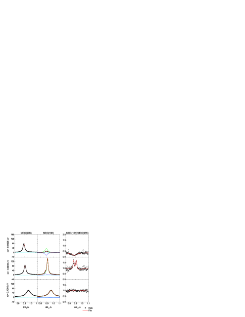
Figure 1: The representative MDC as a function of the momentum measured from the $(\pi,\pi)$ point along the tilt angle $\theta=20^{\circ}$. The dots are the experimental data and the solid red lines are the fitting. The first and second columns show the fitting in the normal state at $T=97$ and in the SC state at $T=16$ K, respectively. The last column is the MDC ratios of SC to normal states.

The most crucial is the observation of the particle-hole mixing in the momentum distribution curve (MDC) in SC state by the high resolution laser ARPES which opened up a new window to probe the fundamental physics of high temperature SC.Zhang12prb ; Yun11prb See the middle row of Fig. 1 which shows the MDC along the cut $\theta=20^{\circ}$. We use the angle $\theta$ from the diagonal direction to label each cut in the Brillouin zone as shown in Fig. 2. The actual momentum paths are shown by the slightly curved thick bars along each cut. The $k_{\perp}$ is the distance from the $(\pi,\pi)$ point. The first and second columns of the Fig. 1 show the normal state at $T=97$ and SC state at $T=16$ K, respectively. For the second column, the red, green, and blue represent the total, particle, and hole contributions. Notice that in addition to the main peak near $k_{\perp}a/\pi\approx 0.91$ from the original quasi-particle branch, there exists the secondary peak at $k_{\perp}a/\pi\approx 0.87$ from the hole branch. This is a direct observation of the particle-hole mixing deep in the SC state and can be utilized to obtain the crucial frequency dependence of the self-energy of the cuprates.

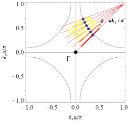
Figure 2: The Fermi surface of Bi2212 in the first Brillouin zone. The blue solid curve is a calculated Fermi-surface and the solid dots are experimentally determined FS at $\theta=0$, 5, 10, 15, 20, and 25 degrees. $k_{\perp}$ is the distance from the $(\pi,\pi)$ point. The thick bars along each cut indicate the ranges of experimentally measured ARPES MDC data.

Another crucial point is that the Eliashberg analysis of the ARPES data can distinguish the Eliashberg functions in the diagonal and off-diagonal (pairing) channels, $\alpha^{2}F^{(+)}(\mathbf{k},\mathbf{k}^{\prime},\omega)$ and $\alpha^{2}F^{(-)}(\mathbf{k},\mathbf{k}^{\prime},\omega)$, respectively. See Eq. (5) below. To our knowledge, this separation can only be accomplished from analysis of ARPES data. This is particularly interesting because it offers a way to disentangle the boson spectrum. As Anderson commented,Anderson07science the strong onsite repulsion $U$ causes the broad structure in the electrons’ energy distribution functions. This may naively be described by coupling to a broad boson spectrum which, however, doesn’t help with pair binding. In the Eliashberg framework, $\alpha^{2}F^{(+)}(\mathbf{k},\mathbf{k}^{\prime},\omega)$ and $\alpha^{2}F^{(-)}(\mathbf{k},\mathbf{k}^{\prime},\omega)$ represent, respectively, the boson spectrum which electrons are coupled to and that which helps with pair binding.

This is an extension of the tunneling experiments and analysis with which it was definitely established that the pairing in metals like Pb is through exchange of phonons.McMillan65prl It should be remembered that to get reliable information, it was necessary to have measurements of conductance at different temperatures and range of voltages of the order of the cut-off energy in the phonon spectrum to an accuracy of 0.2 %. Since the cut-off is an order of magnitude higher and the angle-dependence of the spectra is crucial for the cuprates, the demands on the quality of the data are only being recently met through ultra-high resolution and stability of laser based ARPES.

III.1 Deduced diagonal self-energy

The quantity that we will focus is the angle and frequency dependence of the diagonal self-energy $\Sigma(\theta,\omega)$. We refer to the papers Ref. Bok10prb, ; Yun11prb, ; Zhang12prb, for the detailed procedure for inverting ARPES. A very similar approach using ARPES only along the nodal direction was reported in Ref. Schachinger08prb, . Here we only provide a summary of the results. We were able to deduce the angle and frequency dependence of the normal state self-energy $\Sigma(\theta,\omega)$ at $T=107$ K. There is no perceptible dependence on $|{\mathbf{k}}-{\mathbf{k}}_{F}|$ as can be seen from the first column of Fig. 1 in that the normal state MDC are almost perfect Lorentzian. The obtained self-energies are shown in Fig. 3. The subscripts 1 and 2 stand for the real and imaginary parts, respectively. The plot 3(a) is the results obtained using a tight-binding dispersion $\xi(\mathbf{k})$, while 3(b) is obtained using a linear dispersion. It is given for comparison to check the effects of different bare dispersions. Here the bare dispersion $\xi(\mathbf{k})$ actually represents the renormalized dispersion but without including the effects of the putative interaction $\alpha^{2}F$.

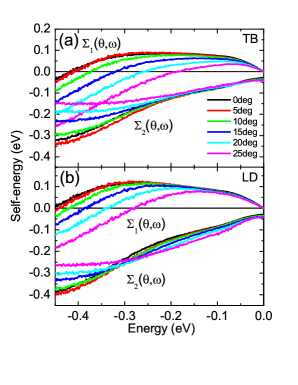
Figure 3: The real $\Sigma_{1}$ and imaginary $\Sigma_{2}$ parts of self-energy at $T=107K$ as a function of energy $\omega$ for the tilt angles $\theta$ = 0, 5, 10, 15, 20, and 25 degrees with respect to the diagonal cut in the Brillouin zone. Plot (a) is the results obtained using a tight-binding dispersion $\xi(\mathbf{k})$ while (b) is given to compare the results if a linear extrapolation of the band-structure from that near the Fermi energy is adopted.

Two points are to be noticed about the self-energy at $T=107$ K in the normal state: (1) In the low energy regime $(-0.05\lesssim\omega<0)$, the $\Sigma_{1}(\theta,\omega)$ is almost angle independent, and (2) the zero crossing energy $\omega_{0}=|\omega|$ of $\Sigma_{1}(\theta,\omega)$, that is, $\Sigma_{1}(\theta,-\omega_{0})=0$, decreases monotonically as the angle increases. From $\omega_{0}\approx 0.4$ at $\theta=0$ to $\omega_{0}\approx 0.2$ eV at $\theta=25^{\circ}$. In order to understand these results in terms of the effective interaction $\alpha^{2}F$, recall that the $\Sigma_{1}$ is the shift of the renormalized dispersion from the bare one and is proportional to the $\alpha^{2}F$ within the Eliashberg framework. Also recall that the zero of the real part of a causal function corresponds to a peak (or, saturation) of the imaginary part which in turn corresponds to the cutoff of $\alpha^{2}F$. Then the point (1) implies that the $\alpha^{2}F$ is almost angle independent below $~{}0.05$ eV, and (2) implies that the cutoff energy of the Eliashberg function decreases as the angle increases. These are indeed what we found by the maximum entropy method to invert the $d$-wave Eliashberg equation as given in Eq. (1). See the Fig. 5 below. This will be discussed in the next section.

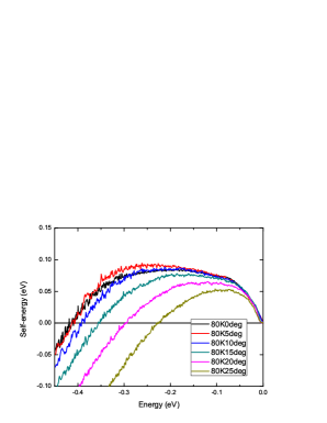
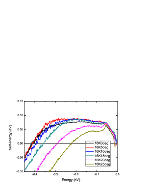
Figure 4: The real part of the self-energy. (a) is at $T=80$ K slightly below $T_{c}$, and (b) is at $T=16$ K deep in the SC state. Notice that the two observations made at $T=107$ K are also valid at $T=80$ K; the overlap of the curves for small $\omega\gtrsim-0.05$ eV and the decreasing cutoff energy as a function of the angle. Only in the low temperature the SC induced features show up near $-0.02$ and $-0.05$ eV as can be seen from the plot (b).

We now consider how the angle and frequency dependence of the self-energy vary in the SC state. The real part of the self-energy is shown in Fig. 4. Plot 4(a) is at $T=80$ K just below $T_{c}=89$ K, and (b) is deep in the SC state at $T=16$ K. At $T=80$ K, above two observations at $T=107$ K remain valid, that is, the angle independence of $\Sigma_{1}$ in the low energy and decreasing zero crossing energy as the angle increases from the nodal cut. Only deep in the SC state at $T=16$ K as shown in Fig. 4(b) the SC induced changes in the $\Sigma_{1}$ show up. Two structures emerge near $\omega\approx-0.02$ and $-0.05$ eV. Both are consistent with the $d$-wave pairing gap. The two structures imply that the $\alpha^{2}F$ will exhibit two additional features to that in the normal state. To that we turn now.

III.2 Eliashberg function

While the self-energy extraction does not need an underlying theory except for the observation that cuprate superconductivity follows the $d$-wave BCS theory, the description of the self-energy in terms of boson spectrum requires that the Eliashberg-type theory is valid for the cuprates. Although it is not yet settled if the Eliashberg formalism is valid for the cuprates (see below in Sec. V), we will use it to discuss the boson spectrum. Please see Ref. Yun11prb, for the results at various temperatures and angles.

The Eliashberg equation is given by

$$\widetilde{\Sigma}(\mathbf{k},\omega)=\int^{\infty}_{-\infty}d\epsilon\int^{\infty}_{-\infty}d\epsilon^{\prime}\frac{f(\epsilon)+n(-\epsilon^{\prime})}{\epsilon+\epsilon^{\prime}-\omega-i\delta}$$

$$\times\sum_{\mathbf{k^{\prime}}}A_{S}(\mathbf{k^{\prime}},\epsilon)\alpha^{2}F^{(+)}(\mathbf{k},\mathbf{k^{\prime}},\epsilon^{\prime}),$$

$$X(\mathbf{k},\omega)=\int^{\infty}_{-\infty}d\epsilon\int^{\infty}_{-\infty}d\epsilon^{\prime}\frac{f(\epsilon)+n(-\epsilon^{\prime})}{\epsilon+\epsilon^{\prime}-\omega-i\delta}$$

$$\times\sum_{\mathbf{k^{\prime}}}A_{X}(\mathbf{k^{\prime}},\epsilon)\alpha^{2}F^{(+)}(\mathbf{k},\mathbf{k^{\prime}},\epsilon^{\prime}),$$

$$\phi(\mathbf{k},\omega)=\int^{\infty}_{-\infty}d\epsilon\int^{\infty}_{-\infty}d\epsilon^{\prime}\frac{f(\epsilon)+n(-\epsilon^{\prime})}{\epsilon+\epsilon^{\prime}-\omega-i\delta}$$

$$\times\sum_{\mathbf{k^{\prime}}}A_{\phi}(\mathbf{k^{\prime}},\epsilon)\alpha^{2}F^{(-)}(\mathbf{k},\mathbf{k^{\prime}},\epsilon^{\prime}),$$ (1)

where $f$ and $n$ are the Fermi and Bose distribution functions, respectively.

$$\Sigma(\mathbf{k},\omega)=\widetilde{\Sigma}(\mathbf{k},\omega)+X(\mathbf{k},\omega)$$ (2)

is the diagonal self-energy and $\phi(\mathbf{k},\omega)$ is the off-diagonal self-energy. The spectral functions are given by

$$A_{S}(\mathbf{k},\epsilon) = -\frac{1}{\pi}Im\frac{W}{W^{2}-Y^{2}-\phi^{2}}=A_{S}(\mathbf{k},-\epsilon),$$

$$A_{X}(\mathbf{k},\epsilon) = -\frac{1}{\pi}Im\frac{Y}{W^{2}-Y^{2}-\phi^{2}}=-A_{X}(\mathbf{k},-\epsilon),$$

$$A_{\phi}(\mathbf{k},\epsilon) = -\frac{1}{\pi}Im\frac{\phi}{W^{2}-Y^{2}-\phi^{2}}=-A_{\phi}(\mathbf{k},-\epsilon),$$

$$A(\mathbf{k},\epsilon) = A_{S}(\mathbf{k},\epsilon)+A_{X}(\mathbf{k},\epsilon).$$ (3)

We use

$$W(\mathbf{k},\omega)=\omega-\widetilde{\Sigma}(\mathbf{k},\omega),$$

$$Y(\mathbf{k},\omega)=\xi(\mathbf{k})+X(\mathbf{k},\omega).$$ (4)

The diagonal and off-diagonal Eliashberg functions are given by

$$\alpha^{2}F^{(+)}(\mathbf{k},\mathbf{k^{\prime}},\epsilon^{\prime})=\alpha_{ch}^{2}F_{ch}(\mathbf{k},\mathbf{k^{\prime}},\epsilon^{\prime})+\alpha_{sp}^{2}F_{sp}(\mathbf{k},\mathbf{k^{\prime}},\epsilon^{\prime}),$$

$$\alpha^{2}F^{(-)}(\mathbf{k},\mathbf{k^{\prime}},\epsilon^{\prime})=\alpha_{ch}^{2}F_{ch}(\mathbf{k},\mathbf{k^{\prime}},\epsilon^{\prime})-\alpha_{sp}^{2}F_{sp}(\mathbf{k},\mathbf{k^{\prime}},\epsilon^{\prime}),$$

$$\alpha^{2}F^{(\pm)}(\theta,\epsilon^{\prime})\equiv\left\langle\frac{\alpha^{2}(\theta,\theta^{\prime})}{v_{F}(\theta^{\prime})}F^{(\pm)}(\theta,\theta^{\prime},\epsilon^{\prime})\right\rangle_{\theta^{\prime}},$$ (5)

where $v_{F}(\theta^{\prime})$ is the angle dependent Fermi velocity and the bracket implies the angular average over $\theta^{\prime}$. The subscripts $ch$ and $sp$ represent, respectively, the time-reversal symmetry conserving and breaking interactions. For example, to the latter (former) belong the spin (charge) and current interactions. For more technical details, please refer to the references Ref. Yun11prb, ; Hong12unp, .

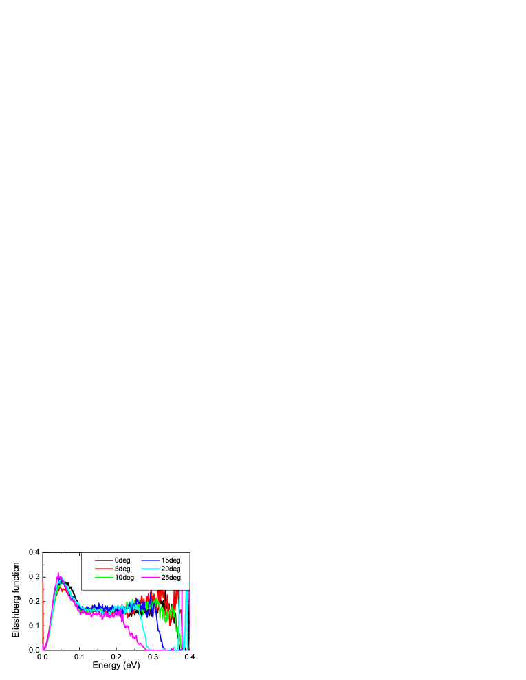
Figure 5: The diagonal Eliashberg function $\alpha^{2}F^{(+)}(\theta,\omega)$ at $T=107$ K extracted from the self-energy shown in Fig. 3. The curves overlap below $0.02$ eV and the cutoff energy decreases as the angle increases from the nodal cut.

Using the deduced self-energy, we have inverted the $d$-wave Eliashberg equation for the normal state self-energy to deduce the normal Eliashberg function $\alpha^{2}F^{(+)}(\theta,\epsilon)$. The results are shown in Fig. 5. The deduced $\alpha^{2}F^{(+)}(\theta,\epsilon)$ behaves as expected before in Section III.1. It is independent of angle to an accuracy of about 10% below an energy of about 0.2 eV. Above this energy there is an angle dependent cutoff $\omega_{c}(\theta)$. $\omega_{c}$ decreases as the angle increases from $\sim 0.4$ eV at $\theta=0$ to $\sim 0.2$ eV at $\theta=25$ degrees. That is, the only angle dependence of the Eliashberg function in the normal state is the cutoff $\omega_{c}(\theta)$.

Now, we consider the diagonal Eliashberg function in the SC state.Yun11prb The principal conclusions are that along the nodal cut ($\theta=0$) the fluctuations below $T_{c}$, within the uncertainty of determination, are almost unchanged from the fluctuations above $T_{c}$. For larger energies above about 0.1 eV, they are similarly unchanged from the fluctuations above $T_{c}$. On the other hand, there is a growth of the peak around 50 meV for the lower temperatures and larger angles, and the emergence of a new peak at about $10-15$ meV. These features are probably related to the loss of dissipation due to the opening of the superconducting gap and would be interesting to study theoretically in greater detail.

The deduced $\alpha^{2}F^{(+)}(\theta,\omega)$ discussed above are consistent with an earlier deduction Schachinger08prb from ARPES spectrum in the same compound, and also qualitatively consistent with the deduction from optical conductivity spectrumHwang07prb ; Heumen09prb , which preferentially weights the nodal quasi-particles because of their larger Fermi velocity.

Now, let us consider the Eliashberg function along the pairing channel, $\alpha^{2}F^{(-)}(\theta,\omega)$. The information on the pairing self-energy is contained only in the difference in the ARPES spectra in the superconducting state and the normal state. This difference is expectedYun11prb to be less than 1% above an energy of a few times the superconducting gap. Above such energy, the noise in the data is at present significantly larger than 1%. Therefore, we have not been able to extract the pairing self-energy and to directly deduce $\alpha^{2}F^{(-)}(\omega)$ from the data over the full energy range of 0.4 eV. But it would be ideal to have data which is about 1/2 an order of magnitude better to completely settle the shape of $\alpha^{2}F^{(-)}(\theta,\epsilon)$.

Determination of the off-diagonal Eliashberg function $\alpha^{2}F^{(-)}(\theta,\epsilon)$ offers perhaps the best way to decide among the proposed ideas. In the loop current idea the $\alpha^{2}F^{(+)}(\theta,\epsilon)$ and $\alpha^{2}F^{(-)}(\theta,\epsilon)$ have the same frequency dependence, while they are different in the spin fluctuation scenario.

IV Discussion of Results

In this section, we discuss the implications of the finding that the Eliashberg function $\alpha^{2}F^{(+)}(\theta,\omega)$ is nearly independent of $\theta$ in the normal state and just below $T_{c}$.Choi11fop It should be remembered again that the superconducting $T_{c}$ is the property of the normal states. Indeed the normal state self-energy just above $T_{c}$ includes all forms of scattering, both spin-dependent as well as spin-independent scatterings from all initial ${\mathbf{k}}$ to all final momenta ${\mathbf{k}^{\prime}}$. Given this, the crucial issue to address is how fluctuations which lead to a nearly $\theta$-independent $\alpha^{2}F(\theta,\omega)$ are reconcilable with the same fluctuations promoting the $d$-wave pairing.

The inadequacy of the AF fluctuations in this regard was given previously.Choi11fop Although the pairing Eliashberg function has not been determined separately, the deduced diagonal Eliashberg function alone is enough to reach this conclusion. The idea is that in the AF spin fluctuation scenario the spin susceptibility $\chi(\mathbf{q},\omega)$ provides both $\alpha^{2}F^{(\pm)}$: the $s$- and $d$-wave projection of the spin susceptibility yield $\alpha^{2}F^{(+)}$ and $\alpha^{2}F^{(-)}$, respectively. The nearly $\theta$ independent $\alpha^{2}F^{(+)}$ implies a small correlation length $\xi/a\lesssim 1$, where $a$ is the lattice constant. The INS results on YBaCuO indeed found a small AF correlation length $\xi/a\lesssim 1$ near optimal doping concentration.Balatsky99prl The small correlation length means a small $d$-wave projection in the AF spin fluctuation scheme. Then, if one interprets the deduced $\alpha^{2}F^{(+)}(\theta,\omega)$ in terms of the AF fluctuations, s/he can not escape from the conclusion of a small $d$-wave projection component and the low $T_{c}$ smaller than 10 K.

The prospect of the loop current fluctuations was also discussed in Ref. Choi11fop, . The idea is that although the fluctuation spectrum is nearly momentum independent, the coupling vertex has a sufficiently large $d$-wave component in the loop current fluctuations scenario.Aji10prb Here we will add arguments against the AF fluctuation scenario deep in the SC state.

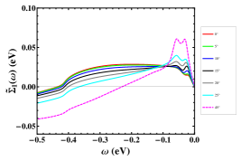
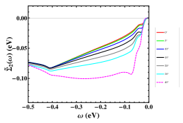
Figure 6: The symmetric part of the self-energy computed from the Vignolle spectrum of La_2-xSr_xCuO₄. (a) is the real part and (b) is the imaginary part. One should compare the plot (a) with the Fig. 4(b). See the text for more details.

The extracted real part of the diagonal self-energy at $T=16$ K is shown in Fig. 4(b). Two observations were made: (1) almost angle independent $\Sigma_{1}(\theta,\omega)$ in the low energy except for the SC induced features near $\omega\approx-0.02$ and $-0.05$ eV, (2) decreasing zero crossing energy $\omega_{0}$ as a function of the angle. To check if the two observations can be explained by the AF spin fluctuation idea, we chose the simplest system where the magnetic spectrum is well known. We took the Vignolle spectrum of single layer La_2-xSr_xCuO₄ with $x=0.16$ from INSVignolle07naturephys for the $\alpha^{2}F_{sp}$ and $\alpha^{2}F_{ch}=0$ for Eq. (5). Although the ARPES results were extracted from the Bi2212, we believe in the commonality of the cuprates phenomenology and trust that the deduced ARPES can certainly be compared with the INS results.

These were solved self-consistently without assuming a separable $\mathbf{k},\omega$ form or particular momentum dependence of the pairing self-energy $\phi(\mathbf{k},\omega)$. Details are reported in Ref. Hong12unp, . The symmetric part of the diagonal self-energies are shown in Fig. 6. Plots 6(a) and (b) are the real and imaginary parts, respectively. Clearly the peak features of $\widetilde{\Sigma}_{1}$ around $30-70$ meV go together with the decreasing zero crossing energy $\omega_{0}$ as a function of the angle. It is because the sharp $\alpha^{2}F$ peak at $(\pi,\pi)$ is most effective in scattering the particles near the antinodal region ($\theta\approx 45^{\circ}$). The effects of the scatterings off the $(\pi,\pi)$ peak show up as a fast increase of $-\Sigma_{2}(\theta\approx 45,\omega)$ as $-\omega$ increases. $-\Sigma_{2}(\omega)$ then makes a shallow peak and begins to decrease. Recall that to a peak in the imaginary part of a causal function corresponds a zero crossing of the real part of that function. This is the reason why the peak features around $30-70$ meV go together with the decreasing zero crossing energy in the AF spin fluctuations scenario. As shown in Fig. 6(a), the peak feature around $30-70$ meV is too strong and the decrease of the zero crossing energy is too slow compared with the ARPES results shown in Fig. 4(b).

The previous conclusion from the Ref. Choi11fop, was that if the fluctuations coupling to fermions revealed in ARPES experiments were AF fluctuations, $T_{c}$ would have been less than 10 K. The reason is that if the correlation length of fluctuations is not much larger than the lattice constant, the projection to $d$-wave scattering is small compared to the average or $s$-wave scattering. Hence, follows a very small $T_{c}$. The SC state analysis briefed here reinforces the previous conclusion from the normal state analysis that it is difficult to understand the results of the ARPES analysis within the AF spin fluctuations idea.

This view is in stark contrast with the result reported by Dahm $et~{}al.$Dahm09naturephys As discussed before in Sec. II, they analyzed the charge- and spin-excitation spectra determined by the ARPES and inelastic neutron scatterings on the same crystal of YBa₂Cu₃O_6.6 and claimed that a self-consistent description of both spectra can be obtained by adjusting a single parameter, the spin-fermion coupling constant. They suggested that the spin fluctuations have a sufficient strength to mediate high-temperature superconductivity.

We suggest that there is a more stringent test on the spin fluctuation scenario. Because the commensurate and incommensurate spin fluctuations of the Vignolle spectrum have sharp peaks, of about $\xi/a\approx 2-3$ and $6-7$ in the low temperature limit, their scatterings are selective in the momentum space. That is why the peak of the real part self-energy shown in Fig. 6(a) exhibits the strong angle dependence. This, however, does not agree with what was deduced from the ARPES analysis. The detailed frequency and angle dependence of the self-energy need to be performed for the AF spin fluctuations scenario before claiming it as the pairing interaction.

V outlooks

In hindsight, the remarkable success of the BCS theory owes much to the smallness of the ratio of the phonon energy to the Fermi energy, $\hbar\omega_{D}/\epsilon_{F}\ll 1$. Assured by the Migdal theorem, it enables one to do the controlled perturbation expansion. Moreover, this small ratio also tames the Coulomb repulsion into the benign Coulomb pseudo-potential, $\mu^{*}$, while at the same time this retardation effect limits the $T_{c}$.

For pairing due to the electron-electron interaction, one can certainly try to invoke the Migdal theorem thanks to the small ratio of the collective energy like the spin fluctuation energy $\omega_{sf}$ to the Fermi energy $\epsilon_{F}$. But there is no rigorous grounds for it.Abanov03aip ; Hertz76ssc The difficulty comes from the fact that in the electron system the collective degrees of freedom like the spin fluctuations are composed of the very same electrons that are being paired. One should come up with a scheme to deal with this situation more systematically.

The determination of the frequency dependence of pairing was motivated by the idea that it could differentiate among the proposed theories. The proponents for the RVB theory argue that the pairing in the cuprates does not have the low energy dynamics. On the other hand, the other group for the pairing glue like the spin fluctuations or loop current fluctuations argues that the pairing interaction has the low energy dynamics set by the relevant fluctuations. However, even in the RVB theory the claim of no low energy dynamics is not accepted unanimously. Attempts to go beyond the mean-field RVB approach typically invoke the gauge fluctuations as a way to enforce the no double occupancy which generates significant low energy dynamics.Lee06rmp But, this dynamics of gauge fluctuations is difficult to compute to compare with experiments quantitatively.

In this regard, two more features of the ARPES analysis will be valuable: The angle dependence of the self-energy and the separate determination of the two Eliashberg functions, the diagonal and off-diagonal $\alpha^{2}F^{(\pm)}$. The angle dependence of the self-energy can be a stringent test as we argued in the previous section. Also the possibility of independent extraction of $\alpha^{2}F^{(+)}$ and $\alpha^{2}F^{(-)}$ from the diagonal and off-diagonal self-energies, $\Sigma$ and $\phi$, respectively, is a unique advantage of the ARPES analysis. As we stand now, determination of $\phi(\mathbf{k},\omega)$ suffers from loss of accuracy. As we commented before, the information on the pairing self-energy is contained in the difference of the ARPES intensities between the normal and SC states. It would be ideal to have ARPES data of about half an order of magnitude better to fix the pairing Eliashberg function $\alpha^{2}F^{(-)}$. This perhaps gives the best way to decide among the proposed ideas.

Differences among the ideas should also show up in the excitations of the proposed states. The elementary excitations in the RVB state have reversed charge-statistics relations: They are neutral spin-1/2 fermions and charge $\pm e$ spinless bosons, analogous to the solitons in polyacetylene.Kivelson87prb In the spin fluctuations idea they are the usual fermions and $S_{z}=\pm 1$ spins. The excitations in the loop current state are also being explored.Li12naturephys

The phase diagram also offers a way to differentiate among proposals. The RVB theory predicted a phase diagram where the pseudogap temperature $T^{*}$ and SC critical temperature $T_{c}$ lines merge together as the doping concentration increases. This is in contrast to the phase diagram of the pairing glue camp where the $T^{*}$ and $T_{c}$ lines cross each other and $T^{*}$ line continues inside the $T_{c}$ dome. In both scenarios the nature of the pseudogap phase below $T^{*}$ determines the origin of the pairing. In this regard, the nature of the pseudogap is the key. And again, pseudogap, anomalous normal state, and superconductivity should be understood in their totality. That is the question.

- (1) Bardeen, J., Cooper, L. N. & Schrieffer, J. R. Theory of superconductivity. Phys. Rev. 108, 1175–1204 (1957).
- (2) Gough, C. E. et al. Flux quantization in a high-tc superconductor. Nature 326, 855 (1987).
- (3) Wollman, D. A., Van Harlingen, D. J., Lee, W. C., Ginsberg, D. M. & Leggett, A. J. Experimental determination of the superconducting pairing state in ybco from the phase coherence of ybco-pb dc squids. Phys. Rev. Lett. 71, 2134–2137 (1993).
- (4) Anderson, P. W. The resonating valence bond state in la2cuo4 and superconductivity. Science 235, 1196–1198 (1987).
- (5) Anderson, P. W. Is there glue in cuprate superconductors? Science 316, 1705–1707 (2007).
- (6) Monthoux, P., Pines, D. & Lonzarich, G. G. Superconductivity without phonons. Nature 450, 1177–1183 (2007).
- (7) Dahm, T. et al. Strength of the spin-fluctuation-mediated pairing interaction in a high-temperature superconductor. Nature Phys. 5, 217 (2009).
- (8) Scalapino, D. J. A common thread. Physica C 470, S1 – S3 (2010).
- (9) Varma, C. M. Theory of the pseudogap state of the cuprates. Phys. Rev. B 73, 155113 (2006).
- (10) Aji, V. & Varma, C. M. Theory of the quantum critical fluctuations in cuprate superconductors. Phys. Rev. Lett. 99, 067003 (2007).
- (11) Aji, V., Shekhter, A. & Varma, C. M. Theory of the coupling of quantum-critical fluctuations to fermions and -wave superconductivity in cuprates. Phys. Rev. B 81, 064515 (2010).
- (12) McMillan, W. L. & Rowell, J. M. Lead phonon spectrum calculated from superconducting density of states. Phys. Rev. Lett. 14, 108–112 (1965).
- (13) Maier, T. A., Poilblanc, D. & Scalapino, D. J. Dynamics of the pairing interaction in the hubbard and models of high-temperature superconductors. Phys. Rev. Lett. 100, 237001 (2008).
- (14) Eliashberg, G. M. Interactions between electrons and lattice vibrations in a superconductor. JETP 11, 696 (1960).
- (15) Abrahams, E. The evolution of high temperature superconductivity: Theory perspective. In Cooper, L. N. & Feldman, D. (eds.) BCS: 50 Years, 439–469 (World Scientific, Singapore, 2011). Also in Int. J. Mod. Phys. B 24, 4150 (2010).
- (16) Lee, P. A. From high temperature superconductivity to quantum spin liquid: Progress in strong correlation physics. Rep. Prog. Phys. 71, 012501 (2008).
- (17) Eschrig, M. The effect of collective spin-1 excitations on electronic spectra in high-t c superconductors. Advances in Physics 55, 47–183 (2006).
- (18) Choi, H.-Y., Varma, C. M. & Zhou, X. Superconductivity in the cuprates: Deduction of mechanism for d-wave pairing through analysis of arpes. Front. Phys. 6, 440–449 (2011).
- (19) Carbotte, J. P., Timusk, T. & Hwang, J. Bosons in high-temperature superconductors: An experimental survey. Rep. Prog. Phys. 74, 066501 (2011).
- (20) Hackl, R. & Hanke, W. Towards a better understanding of superconductivity at high transition temperatures. Eur. Phys. J.: Special Top. 188, 3–14 (2010).
- (21) Zaanen, J. A modern, but way too short history of the theory of superconductivity at a high temperature. ArXiv e-prints (2010). eprint 1012.5461.
- (22) Norman, M. R. Cuprates - An Overview. ArXiv e-prints (2011). eprint 1108.3140.
- (23) Aimi, T. & Imada, M. Does simple two-dimensional hubbard model account for high-tc superconductivity in copper oxides? J. Phys. Soc. Jap. 76, 113708 (2007).
- (24) Kyung, B., Senechal, D. & Tremblay, A. . S. Pairing dynamics in strongly correlated superconductivity. Phys. Rev. B 80, 205109 (2009).
- (25) Abanov, A., Chubukov, A. V. & Schmalian, J. Quantum-critical theory of the spin-fermion model and its application to cuprates: Normal state analysis. Adv. Phys. 52, 119–218 (2003).
- (26) Khatami, E., Macridin, A. & Jarrell, M. Validity of the spin-susceptibility “glue” approximation for pairing in the two-dimensional hubbard model. Phys. Rev. B 80, 172505 (2009).
- (27) Varma, C. M., Littlewood, P. B., Schmitt-Rink, S., Abrahams, E. & Ruckenstein, A. E. Phenomenology of the normal state of cu-o high-temperature superconductors. Phys. Rev. Lett. 63, 1996–1999 (1989).
- (28) Schachinger, E. & Carbotte, J. P. Finite band inversion of angular-resolved photoemission in and comparison with optics. Phys. Rev. B 77, 094524 (2008).
- (29) Hwang, J., Timusk, T., Schachinger, E. & Carbotte, J. P. Evolution of the bosonic spectral density of the high-temperature superconductor . Phys. Rev. B 75, 144508 (2007).
- (30) van Heumen, E. et al. Optical determination of the relation between the electron-boson coupling function and the critical temperature in high-t[sub c] cuprates. Phys. Rev. B 79, 184512 (2009).
- (31) Bok, J. M. et al. Momentum dependence of the single-particle self-energy and fluctuation spectrum of slightly underdoped from high-resolution laser angle-resolved photoemission. Phys. Rev. B 81, 174516 (2010).
- (32) Yun, J. H. et al. Analysis of laser angle-resolved photoemission spectra of ba2sr2cacu2o8+δ in the superconducting state: Angle-resolved self-energy and the fluctuation spectrum. Phys. Rev. B 84, 104521 (2011).
- (33) Zhang, W. et al. Extraction of normal electron self-energy and pairing self-energy in the superconducting state of the bi2sr2cacu2o8 superconductor via laser-based angle-resolved photoemission. Phys. Rev. B 85, 064514 (2012).
- (34) Hong, S. H. & Choi, H.-Y. The angle-resolved normal and anomalous self-energies for optimal lsco supercondcutors: Eliashberg calculation with vignolle spectrum. Phys. Rev. B (2012). Unpublished.
- (35) Balatsky, A. V. & Bourges, P. Linear dependence of peak width in (q,) vs for superconductors. Phys. Rev. Lett. 82, 5337–5340 (1999).
- (36) Vignolle, B. et al. Two energy scales in the spin excitations of the high-temperature superconductor la2-xsrxcuo4. Nature Phys. 3, 163–167 (2007).
- (37) Hertz, J. A., Levin, K. & Beal-Monod, M. T. Absence of a migdal theorem for paramagnons and its implications for superfluid he3. Solid State Comm. 18, 803–806 (1976).
- (38) Lee, P. A., Nagaosa, N. & Wen, X.-G. Doping a mott insulator: Physics of high-temperature superconductivity. Rev. Mod. Phys. 78, 17–85 (2006).
- (39) Kivelson, S. A., Rokhsar, D. S. & Sethna, J. P. Topology of the resonating valence-bond state: Solitons and high- superconductivity. Phys. Rev. B 35, 8865–8868 (1987).
- (40) Li, Y. et al. Two ising-like magnetic excitations in a single-layer cuprate superconductor. Nature Phys. (2012). Article in Press.