Profile control charts based on nonparametric $\bolds{L}$-1 regression methods

Abstract

Classical statistical process control often relies on univariate characteristics. In many contemporary applications, however, the quality of products must be characterized by some functional relation between a response variable and its explanatory variables. Monitoring such functional profiles has been a rapidly growing field due to increasing demands. This paper develops a novel nonparametric $L$-1 location-scale model to screen the shapes of profiles. The model is built on three basic elements: location shifts, local shape distortions, and overall shape deviations, which are quantified by three individual metrics. The proposed approach is applied to the previously analyzed vertical density profile data, leading to some interesting insights.

, and

T1The content is solely the responsibility of the authors and does not necessarily represent the official views of the NIDA or the NIH.

t2Supported by NSF Grant DMS-09-06568 and a career award from the NIEHS Center for Environmental Health in Northern Manhattan (ES-009089).

t3Supported in part by NIDA Grant P50-DA10075-15.

1 Introduction

Since its initial introduction by Shewart in the 1920s, statistical process control (SPC) has received increasing attention from both academia and industry. Traditional SPC often utilizes a single metric (e.g., mass or length) to characterize products under inspection. For such metrics, lower and upper control limits are then estimated from manufacturing data. For example, such limits could be defined by the mean plus and minus three standard deviations. If its metric falls out of the control limits, it could imply a potential change in the underlying distribution (for stability), or a product could be rejected due to a potential quality deficiency (for conventional quality control).

In traditional SPC, the quality of a product is often assumed to be adequately characterized by univariate characteristics or certain metrics. In recent years, however, there have been increasing needs for profile control charts for which the responses are no longer single measurements but, rather, functions of one or several covariates $X$. Traditional methods handling univariate or multivariate charts are no longer applicable to such functional profile responses [Woodall (2007)]. Several new approaches have been subsequently proposed. One basic class of methods assumes a linear association between a response $Y$ and its covariate $X$ and then constructs the corresponding control charts on the intercept, slope and variance. When linearity is not an option, nonlinear models are usually introduced. The control charts are then built upon one or several model coefficients. Jensen, Birch and Woodall (2008), Jensen and Birch (2009) further consider parametric (linear and nonlinear) mixed effect models to take into account intraprofile correlations. Qiu, Zou and Wang (2010) further consider nonparametric mixed effects modeling Phase II profile monitoring.

In many applications, it is difficult to know a priori the shape of a response profile. Inappropriate shape assumptions can lead to substantial estimation bias. To overcome this difficulty, Reis and Saraiva (2006), Jeong, Lu and Wang (2006), Ding, Zeng and Zhou (2006), Zhou, Sun and Shi (2007) and Chicken, Pignatiello and Simpson (2009) explore nonparametric wavelet models and construct control charts based on a portion of the wavelet coefficients. Since the screening method therein relies only on major wavelet coefficients, any deviations of the other coefficients may be undetectable. Zou, Tsung and Wang (2008) also explore an alternative nonparametric approach for profile monitoring in which the measures within each profile are assumed to be independent.

The above approaches always project the profile information onto a set of parameters, while a more natural method is to utilize the entire information of the target profiles. We hence propose estimating a reference profile based on Phase I data and then monitoring the deviations of individual profiles in Phase II from the reference one. The basic statistical tool we use to model Phase I data is $L$-1 regression assuming a nonparametric location-scale model with a general class of error structure. Compared with traditional $L$-2 regression, $L$-1 regression is more robust against outliers and heavy-tailed distributions. We refer to Koenker (2005) for an extensive exposition on the properties of $L$-1 regression. Based on the estimated model in Phase I, we propose three deviation measures to monitor individual Phase II profiles in overall location shift, local failure and overall shape deviation. The control limits of the three deviation metrics are determined based on the empirical estimation of their asymptotic distributions.

As an illustrative example, we apply the proposed method to the vertical density profile (VDP) data of Walker and Wright (2002). In that study, the manufacturers of engineered wood boards are very concerned about fiberboard density, which determines the fiberboard’s strength and physical properties. The density ($Y$) is read by a profilometer, a laser device measuring densities at equispaced points ($X$) along a designated vertical line. Each resulting profile consists of 314 density measurements, and the distance between two consecutive measures is 0.002 inch. Figure 1 provides a visual illustration of the data set. These curves are clearly nonlinear, and thus new technologies to monitor these curves are desirable.

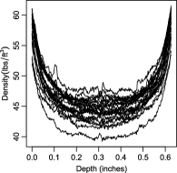
Figure 1: Walker–Wright data.

The rest of our paper is organized as follows. Section 2 introduces a nonparametric location-scale $L$-1 regression with a generalized error structure, as well as the estimation procedure. We then describe in detail how to construct profile control charts utilizing nonparametric $L$-1 regression. The screening is based on three deviation measures, whose asymptotic properties are established. The proposed method is then applied to the VDP data and illustrated in Section 3.1. Section 3.2 compares the proposed method to alternative approaches, and Section 3.3 provides a numerical investigation. Section 4 presents concluding remarks and a discussion. The theoretical regularity conditions for the proposed method are summarized in the Appendix, while the proof of the main theorem is presented in the supplementary materials.

2 Proposed methodology

Two phases, often denoted by Phases I and II, are typically involved in SPC [Woodall (2007)]. The goal in Phase I is to construct the control limits which determine if a process has been in control over the period of time. Phase II then applies these limits to detect a potential change in the underlying distribution (for stability). This paper follows the same convention.

2.1 Modeling Phase I profiles

2.1.1 Representation of Phase I profiles based on a family of nonparametric location-scale models

Suppose there exist $n$ independent Phase I profiles, $\{{\mathbf{Y}}_{i}=(Y_{i,1},Y_{i,2},\ldots,Y_{i,m_{i}}),i=1,\ldots,n\}$, where $m_{i}$ denotes the number of elements. Let $x_{i,j}$ represent the location where $Y_{i,j}$ is taken. For instance, if ${\mathbf{Y}}_{i}$ is a time sequence, then $x_{i,j}$ can be the underlying measurement time. Given this notation, we assume that Phase I profiles follow a nonparametric location-scale model

$$Y_{i,j}=\delta_{i}+\mu(x_{i,j})+s(x_{i,j})e_{i,j},\qquad 1\leq j\leq m_{i},1\leq i\leq n.$$ (1)

Here we define $\delta_{i}=\mbox{median}({\mathbf{Y}}_{i})$ as the marginal median of the $i$th profile, and view it as the profile center. We also assume that, for each profile $i$, the error process $\{e_{i,j}\}_{j\in\mathbb{N}}$ in (1) is an independent copy from a stationary process with a sufficiently general dependence structure (as specified in Condition 1 in the Appendix). Such a proposed error structure is well suited for control chart profiles, mainly because of two factors: (1) it allows for high correlations induced by dense measurements, differentiating it from typical longitudinal data settings, and (2) unlike classical time sequences, it allows the dependence of both left and right neighboring measurements. The details of the error structure are discussed in the Appendix. We further assume that median$(e_{i,j})=0$ and median$(|e_{i,j}|)=1$. Under these assumptions, $\mu(x)$ is the conditional median of a centered profile $[{\mathbf{Y}}(x)-\mbox{median}\{{\mathbf{Y}}(x)\}]$ given the location $x$, where ${\mathbf{Y}}(x)$ is a random profile satisfying model (1). It represents the standard shape of a normative centered response profile, and we call it the reference profile. The function $s(x)$ is the conditional median absolute deviation (MAD) of the centered profile given the location $x$. It measures the extent to which a normative profile can deviate from the reference profile at a given location $x$, and we call this the reference deviation function. Hence, we decompose the profiles into three domains: center, shape, and variability.

2.1.2 Stepwise estimation

The key components of model (1) are the profile centers $\delta_{i}$, a reference profile $\mu(x)$ and a reference deviation function $s(x)$. These can be estimated sequentially as follows.

Step 1: Estimation of $\delta_{i}$

In a simpler case, where all the profiles are measured on a set of fixed evenly-spaced locations with $m_{i}\equiv m$, the profile-specific centers, $\delta_{i}$, can be estimated by taking the sample median over the observed $\{Y_{i,j},j=1,\ldots,m\}$ for each profile. This type of profiling typically occurs in manufacturing studies such as the VDP profiles introduced earlier.

In more general applications, the number of measurements each sequence contains, $m_{i}$, can vary across profiles, the locations $x_{i,j}$ can be unevenly spaced, and their spacing can also vary across profiles. To handle such varying location profiles, we can assume that each measurement time/location is a random draw from an underlying distribution $F(x)$, and the observed locations $x_{i,j}$ are the order statistics of $m_{i}$ random draws. Letting $X$ be the random variable following the distribution $F(x)$, we then define the profile center as $\delta_{i}=\arg\min_{\theta}E_{Y_{i}(X)}|Y_{i}(X)-\theta|$, where $Y_{i}(x)$ is the underlying profile such that $Y_{i,j}=Y_{i}(x_{i,j})$. Note that since $E_{Y_{i}(X)}|Y_{i}(X)-\theta|=E_{X}[E_{Y_{i}(x)}\{|Y_{i}(x)-\theta||X=x\}]$, the individual center $\delta_{i}$ can be estimated by minimizing the sample objective function $\sum_{j}|Y_{i,j}-\theta|\hat{f}(x_{i,j})$, where $\hat{f}(x_{i,j})$ is the density of $X$ at location $x_{i,j}$ and can be estimated from the pooled sample $x_{i,j}$ (over both $i$ and $j$). When $x_{i,j}$ are evenly spaced, $f(x)$ is a uniform density, that is, $f(x_{i,j})=f(x_{i,j^{\prime}})$ for any $j\not=j^{\prime}$. Hence, the center can be simply estimated as the sample median.

Step 2: Estimation of $\mu(x)$

A kernel-based estimation procedure is employed and the algorithm details are as follows. Under the specified error structure and other mild conditions (as listed in the Appendix), the resulting estimated functions are uniformly consistent and asymptotically normal.

Let $K_{b_{n}}(u)=K(u/b_{n})$ be a nonnegative kernel function with bandwidth $b_{n}>0$ that satisfies $\int_{\mathbb{R}}K(u)\,du=1$. We propose the following least absolute deviation (LAD) estimation for the median function $\mu(x)$:

$$\hat{\mu}_{b_{n}}(x)=\mathop{\arg\min}_{\theta}\sum_{i=1}^{n}\sum_{j=1}^{m_{i}}|Y_{i,j}-\delta_{i}-\theta|K_{b_{n}}(x_{i,j}-x).$$ (2)

The estimation equation (2) is a locally constant type. One can also extend it to a locally linear estimate, as in Fan and Gijbels (1996), without much technical difficulty. We settle on the locally constant approach mainly for computational simplicity.

Following Theorem 1 of Wei, Zhao and Lin (2011), $\{\hat{\mu}_{b_{n}}(x)-\mu(x)\}$ contains a bias term of order $O(b^{2}_{n})$. To remove the bias, we adopt a corrective jackknife estimator [Wu and Zhao (2007)]:

$$\tilde{\mu}_{b_{n}}(x)=2\hat{\mu}_{b_{n}}(x)-\hat{\mu}_{\sqrt{2}b_{n}}(x).$$ (3)

The bias-corrected estimator $\tilde{\mu}_{b_{n}}$ is uniformly consistent and normally distributed for any $x$ asymptotically [Wei, Zhao and Lin (2011)].

Step 3: Estimation of $s(x)$

The reference deviation function $s(x)$ is then estimated from the residuals in the preceding step. Notice that $\mbox{median}(|e_{i,j}|)=1$ entails $\mbox{median}(|Y_{i,j}-\delta_{i}-\mu(x)||x_{i,j}=x)=s(x)$. Therefore, we propose the following median quantile estimate of $s(x)$:

$$\hat{s}_{h_{n}}(x)=\mathop{\arg\min}_{\theta}\sum_{i=1}^{n}\sum_{j=1}^{m_{i}}\bigl{|}|Y_{i,j}-\delta_{i}-\tilde{\mu}_{b_{n}}(x)|-\theta\bigr{|}K_{h_{n}}(x_{i,j}-x),$$ (4)

where $h_{n}>0$ is another bandwidth and $\tilde{\mu}_{b_{n}}(x)$ is a bias-corrected jackknife estimator. Similarly, we construct a bias-corrected jackknife estimator of $s(x)$ with

$$\tilde{s}_{h_{n}}(x)=2\hat{s}_{h_{n}}(x)-\hat{s}_{\sqrt{2}h_{n}}(x),$$ (5)

which is uniformly consistent and asymptotically normal, as shown in Wei, Zhao and Lin (2011). This stepwise estimation is also used in He (1997) under the constraint that both $\mu(x)$ and $s(x)$ are linear.

Bandwidth selection

To implement the proposed methods, one needs to select the proper bandwidths $b_{n}$ and $h_{n}$. Popular choices include plug-in methods, cross-validation (CV) and generalized CV methods. Originally developed for independent data, CV methods often tend to undersmooth correlated data [Opsomer, Wang and Yang (2001)]. However, in the absence of universally efficient alternatives, the CV methods are still among the most widely used [Fan and Yao (2003), Li and Racine (2007)]. This paper also adopts the CV approach.

The basic idea is to leave one profile out and fit the model using the remaining profiles. We then choose the optimal bandwidth that minimizes the prediction error. Classical CV methods deal with quadratic losses, whereas here we work with the $L$-1 loss penalty. Hence, we propose selecting the bandwidth $b_{n}$ by minimizing the following modified CV criterion, that is,

$$b^{*}_{n}=\mathop{\arg\min}_{b_{n}}\sum^{n}_{i=1}\sum^{m_{i}}_{j=1}|Y_{i,j}-\delta_{i}-\tilde{\mu}_{b_{n},-i}(x_{i,j})|,$$ (6)

where $\tilde{\mu}_{b_{n},-i}$ is the bias-corrected jackknife estimator of $\mu$ based on all but the $i$th profile. Similarly, we choose $h_{n}$ with

$$h^{*}_{n}=\mathop{\arg\min}_{h_{n}}\sum^{n}_{i=1}\sum^{m_{i}}_{j=1}\bigl{|}|Y_{i,j}-\delta_{i}-\tilde{\mu}_{b_{n}}|-\tilde{s}_{h_{n},-i}(x_{i,j})\bigr{|},$$ (7)

where $\tilde{s}_{h_{n},-i}$ is defined in the same way as $\tilde{\mu}_{b_{n},-i}$.

Alternative smoothing approaches

Other nonparametric estimation methods, such as smoothing splines, wavelets and normalized B-splines, can also be used to estimate $\mu(x)$ and $s(x)$, respectively, in steps 2 and 3. In general, the estimated $\mu(x)$ and $s(x)$ using other smoothing techniques are also consistent, although their limiting distributions need to be investigated separately. The proposed CV criterion can also be adapted to choose other smoothing parameters. We refer to Opsomer, Wang and Yang (2001) for a detailed comparison of various smoothing methods.

2.2 Construct profile control charts

Suppose $\{(x_{l},Y_{l}),l=1,2,\ldots,m^{*}\}$ is a new profile from Phase II, where $m^{*}$ is the number of measurements of the new profile. We would like to test whether it is different from the Phase I profiles. Specifically, we are interested in testing the null hypothesis,

$$H_{0}\dvtx\mbox{The new profile comes from the same profile population,}$$

against the alternative hypothesis $H_{a}$, that the new profile comes from a different population.

Three deviation measures and their control limits

A new profile can differ from the reference profiles in two ways: through a vertical shift or a shape change. We propose three deviation measures: one for the first type and two for the latter. The profile control charts consist of the screening thresholds of the three deviation measures.

To monitor the vertical outliers, we first estimate the center of the new profile, and denote it as $\delta^{*}$. We then standardize it by

$$D=|\delta^{*}-\hat{\mu}_{\delta}|/\hat{s}_{\delta},$$

where $\hat{\mu}_{\delta}$ and $\hat{s}_{\delta}$ are, respectively, the sample median and MAD of the Phase I profile centers $\delta_{i}$’s. The deviation score $D$ then provides a relative ranking of the new profile, from the inside to the outside, with respect to the Phase I profiles. To determine the screening threshold for $D$, we can generate its reference distribution by the empirical (or bootstrap) distribution of the $d_{i}=|\delta_{i}-\hat{\mu}_{\delta}|/\hat{s}_{\delta}$. Consequently, we can use the $(1-\alpha)$th upper quantile of the $d_{i}$’s as the control limit and denote it $c^{(0)}(\alpha)$. Here $\alpha$ is the significance level and will be determined at a later step. If the deviation score $D$ exceeds $c^{(0)}(\alpha)$, then the profile will be singled out due to its outlying location relative to the Phase I profiles.

It is more challenging to screen shape deviations. We first center the profile by $\{Y_{l}^{*}=Y_{l}-\delta^{*},l=1,\ldots,m^{*}\}$. The center of the new profile $Y_{l}^{*}$ is then zero. By construction, the reference profile $\mu(x)$ is also centered at zero, which means there are no systemic distances between the two profiles after the centering step. Consequently, the main differences between $Y_{l}^{*}$ and $\mu(x)$ are only due to their different shapes.

Recall that $\tilde{\mu}_{b_{n}}$ and $\tilde{s}_{h_{n}}$ are the bias-corrected estimates of $\mu(x)$ and $s(x)$. We define

$$\hat{e}_{l}:=\frac{Y_{l}^{*}-\tilde{\mu}_{b_{n}}(x_{l})}{\tilde{s}_{h_{n}}(x_{l})},\qquad 1\leq l\leq m^{*},$$ (8)

which measures the relative deviation of $Y_{l}^{*}$ from the estimated $\tilde{\mu}_{b_{n}}(x_{l})$ given the estimated scale function $\tilde{s}_{h_{n}}(x_{l})$. We thus consider the following deviation measures:

$$T^{(1)}=\max_{1\leq l\leq m^{*}}|\hat{e}_{l}|\quad\mbox{and}\quad T^{(2)}=\sum^{m^{*}}_{l=1}|\hat{e}_{l}|.$$ (9)

The first statistic $T^{(1)}$ measures the maximal local shape deviation of the new profile from the estimated reference profile, while the second score $T^{(2)}$ measures its cumulative shape deviation. The two scores complement each other, since one monitors the overall shape change while the other monitors local perturbations. Together, the scores provide a comprehensive monitoring of shapes. Gardner et al. (1997) also consider estimating a “reference” surface, using the sum of the residuals to detect unusual signals.

To determine the screening thresholds for the two measures, we first need to derive the distributions of $T^{(1)}$ and $T^{(2)}$ under the null hypothesis. Letting $e_{l}=\{Y_{l}-\delta-\mu(x_{l})\}/s(x_{l})$ be the error of the new profile, the theorem cited below establishes the asymptotic distributions of $T^{(1)}$ and $T^{(2)}$. Here $T^{(1)}$ has an asymptotic extreme value distribution [Galambos (1987)] due to its maximum structure, while $T^{(2)}$ is asymptotically normally distributed.

Theorem 1

Let $N_{n}$ be as in Condition 2 (in the Appendix). Define

$$\Xi_{n}=b^{4}_{n}+h^{4}_{n}+\frac{(\log N_{n})^{3/2}}{(N_{n}b_{n})^{1/2}}+\frac{(\log N_{n})^{3/2}}{(N_{n}h_{n})^{1/2}}.$$

Under Conditions 1–4 (in the Appendix), the following statements hold:

Under $H_{0}$, as $n\to\infty,m^{*}\to\infty$,

$$\bigl{[}T^{(1)}-\beta_{m^{*}}\bigr{]}/\gamma_{m^{*}}\Rightarrow Z,$$

where $Z$ has the extreme value distribution $F$, and $(\gamma_{m^{*}},\beta_{m^{*}})_{{m^{*}}\in\mathbb{N}}$ is a nonrandom sequence with $\gamma_{m^{*}}\downarrow 0$, such that $\mathbb{P}\{{\max_{1\leq l\leq m^{*}}}|e_{l}|\leq\gamma_{m^{*}}x+\beta_{m^{*}}\}=F(x)$ for all continuity points $x$ of $F$ and $\Xi_{n}\beta_{m^{*}}/\gamma_{m^{*}}\to 0$.

Let $e_{0}$ be an independent and identically distributed (i.i.d.) copy of $e_{l}$ and Condition 1 (in the Appendix) holds with $q=2$. Assume that the density function of $e_{0}$ is bounded, and further assume that $\Xi_{n}m^{*3/4}\to 0$ as $n,\allowbreak m^{*}\to\infty$. Then, under $H_{0}$, as $n,m^{*}\to\infty$,

$$\frac{T^{(2)}-m^{*}\mu}{\sqrt{m^{*}}}\Rightarrow N(0,\sigma^{2}),$$

where

$$\mu=\mathbb{E}(|e_{0}|)\quad\mbox{and}\quad\sigma^{2}=\operatorname{Var}(|e_{0}|)+2\sum^{\infty}_{l=1}\operatorname{Cov}(|e_{0}|,|e_{l}|)<\infty.$$ (10)

The conditions for Theorem 1 are summarized in the Appendix, and these conditions are rather common in practice. The proofs are presented in the supplementary materials [Wei, Zhao and Lin (2011)].

The limiting behavior of $T^{(1)}$ is substantially determined by the distribution and dependence characteristics of the underlying $e_{l}$. Therefore, it is quite challenging to obtain the critical value (i.e., screening threshold) of $T^{(1)}$ by using Theorem 1 directly. For $T^{(2)}$, on the other hand, although Theorem 1 guarantees its normal limiting distribution through (ii), estimating $\mu$ and $\sigma^{2}$ can be computationally complicated. Hence, we propose estimating the control limits numerically based on the Phase I data. Specifically, we calculate the shape deviation scores as in (9) for individual Phase I profiles that have measurements on $\{x_{l},l=1,\ldots,m^{*}\}$ and denote them $T_{i,1}$ and $T_{i,2}$, respectively. The screening thresholds are then the $(1-\alpha)$th quantiles of $T_{i,1}$ and $T_{i,2}$. We denote the two screening thresholds by $c^{(1)}(\alpha)$ and $c^{(2)}(\alpha)$, respectively. The control limits can be obtained by bootstrapping the Phase I profiles and using the $(1-\alpha)$th bootstrap quantiles as the desired screening thresholds.

The derived control limits are valid due to the following reasons: (1) Despite the difficulties of obtaining asymptotic critical values directly, Theorem 1 establishes the fact that, under $H_{0}$, both statistics $T^{(1)}$ and $T^{(2)}$ converge to certain stable limiting distributions as the number of Phase I profiles goes to infinity. (2) Assuming that the functions $\mu(\cdot)$ and $s(\cdot)$ are known, then, under $H_{0}$, the distribution of $e_{l}$ of the new profile is the same as that of $e_{i,l}$ from the Phase I profiles, where $e_{i,l}=\{Y_{i,l}-\mu(x_{i,l})\}/s(x_{i,l})$. Hence, the limiting distributions of $T^{(1)}$ and $T^{(2)}$ can be well approximated by the empirical distribution of ${\max_{l}}|e_{i,l}|$’s and $\sum_{l}|e_{i,l}|$’s, respectively, with sufficiently large $n$. Due to the uniform convergence of $\tilde{\mu}_{b_{n}}$ and $\tilde{s}_{h_{n}}$, the distribution of $\hat{e}_{i,l}$ is uniformly and sufficiently close to that of $e_{i,l}$, with large enough $n$ and sufficiently small $b_{n}$ and $h_{n}$. Combining the above facts, one can generate the reference distribution of $T^{(1)}$ and $T^{(2)}$ by the empirical (or bootstrap) distributions of $T_{i,1}$ and $T_{i,2}$.

Determining the significance level $\alpha$

In the proceeding steps, we leave the significance level $\alpha$ unspecified and write the three screening thresholds $c^{(0)}(\alpha)$, $c^{(1)}(\alpha)$ and $c^{(2)}(\alpha)$ as functions of $\alpha$. We now choose $\alpha$ such that

(11)

$$\alpha^{*}=\max_{\alpha}\Biggl{\{}\alpha\dvtx\sum_{i=1}^{n}\max\bigl{\{}\mathbf{1}_{\{d_{i}>c^{(0)}(\alpha)\}},\mathbf{1}_{\{T_{i,1}>c^{(1)}(\alpha)\}},\mathbf{1}_{\{T_{i,2}>c^{(2)}(\alpha)\}}\bigr{\}}<n\alpha_{0}\Biggr{\}},$$

where $\alpha_{0}$ is the desired overall significance level. Following the definition above, a profile will be considered as an outlier if it appears unusual in any of the three domains. And $\alpha^{*}$ is the largest value that ensures that the probability of falsely detecting a normative profile is less than $\alpha_{0}$.

Summary of the screening procedure

Suppose $(x_{l},Y_{l})$ is a new profile. Then the screening consists of the following three steps:

Center the profile by its median $\delta^{*}$ and calculate its relative vertical deviation by

$$D=|\delta^{*}-\hat{\mu}_{\delta}|/\hat{s}_{\delta}.$$

Calculate the cumulative and maximal shape deviation of the centered profile, $Y_{l}-\delta^{*}$, with respect to $\tilde{\mu}_{b_{n}}(x)$ and $\tilde{s}_{h_{n}}(x)$:

$$T^{(1)}=\max_{1\leq l\leq m^{*}}\biggl{|}\frac{Y_{l}-\delta^{*}-\tilde{\mu}_{b_{n}}(x_{l})}{\tilde{s}_{h_{n}}(x_{l})}\biggr{|},\qquad T^{(2)}=\sum^{m^{*}}_{l=1}\biggl{|}\frac{Y_{l}-\delta^{*}-\tilde{\mu}_{b_{n}}(x_{l})}{\tilde{s}_{h_{n}}(x_{l})}\biggr{|}.$$

If either of $D$, $T^{(1)}$ and $T^{(2)}$ exceeds its corresponding screening threshold, $c^{(0)}(\alpha^{*})$, $c^{(1)}(\alpha^{*})$ and $c^{(2)}(\alpha^{*})$, respectively, then the profile $(x_{l},Y_{l})$ will be singled out as a potential outlier.

3 Application

3.1 Profile control chart applied to VDP data

We now return to the VDP data to illustrate the proposed profile screening procedure. Recall that the density of the wood board ($Y$) is measured on a dense sequence of depths ($X$) across the board. The VDP data consist of 24 such profiles, and we view them as Phase I profiles. We first calculate the center of $Y_{i}=(Y_{i,1},\ldots,Y_{i,m})$, which is its overall median $\delta_{i}=\mbox{median}(Y_{i})$. The profile-specific centers $\delta_{i}$ represent the overall vertical locations of those profiles and are presented in Figure 2(a).

After centering, we estimate the reference profile and reference deviation functions $\mu(x)$ and $s(x)$ following the proposed estimation procedure. Based on the CV criterion in (6) and (7), the optimal bandwidths for $b_{n}$ and $h_{n}$ are 0.015 and 0.01, respectively. The resulting $\tilde{\mu}_{b_{n}^{*}}(t)$ and $\tilde{s}_{h_{n}^{*}}(t)$ are presented in Figure 2(b) and are depicted as solid (reference profile) and dashed (deviation profiles) curves.

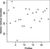
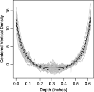
(a)	(b)

Figure 2: VDP profiles. Panel (a) presents the centers of the profiles, while panel (b) plots the centered profiles together with their estimated reference profile (solid curve) and estimated $\mu(x)\pm s(x)$ (dotted lines).

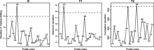
Figure 3: Profile charts of relative vertical deviation and post-centering maximal and cumulative deviations. The dotted lines are determined control limits.

Following the proposed method to construct the control charts, we first calculate the relative vertical deviation scores ($d_{i}$) of the 24 profiles (plotted in the left panel of Figure 3). We then calculate the defined cumulative and maximal deviation scores ($T_{i,1}$ and $T_{i,2}$) for 24 profiles (plotted in the middle and the right panels of Figure 3). The control limits are determined by assuming a significance level $\alpha=0.03$ for each deviation score, which yields an overall significance level $\alpha_{0}=0.12\approx 3/24$. The resulting screening thresholds are 2.99, 7.94 and 663.6, respectively. These control limits are presented by the gray dotted horizontal lines in Figure 3. As shown in Figure 3, Profile A6 is associated with the largest vertical deviation, Profile A3 is the farthest outlier in the maximal shape deviation, while Profile B6 has the largest cumulative shape deviation of all the centered profiles. Although they are assumed to be normative profiles, these profiles provide insights on what the maximum tolerated vertical and shape deviations are. We plot these curves in their original forms in Figure 4. It is clear that Profile A6 has a lower vertical density than all the other profiles, Profile B6 is “too flat” in the center section compared to the rest

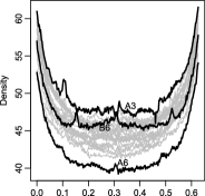
Figure 4: Three profiles associated with the largest $D$, $T^{(1)}$ and $T^{(2)}$.

of the profiles, while Profile A3 has stronger local turbulence than others. Although the VDP data have been used in various studies, our conclusion provides some new insights into the data set.

3.2 Comparisons with other approaches

The VDP data have been investigated by many others. Most approaches are based on linear profile assumptions, as in Woodall et al. (2004), Kim, Mahmoud and Woodall (2003), Mahmoud et al. (2007), Kang and Albin (2000) and Zhu and Lin (2010). Although those linear models may be applicable in some situations, they are clearly inappropriate for the VDP data due to their nonlinear nature. Other nonlinear profile approaches, on the other hand, tend to be more complicated, and some are hard to implement in practice. Two of the most relevant approaches to our work are the bathtub model proposed by Williams, Woodall and Birch (2007) and the $\chi^{2}$ control charts of Zhang and Albin (2009) and Shiau et al. (2009). We elaborate these authors’ approaches below and discuss how they differ from our methods.

Williams, Woodall and Birch (2007) fit a bathtub function

$$f(x_{ij},\beta)=\cases{a_{1}(x_{ij}-c)^{b_{1}}+d,&\quad$x_{j}>c$;\cr a_{2}(x_{ij}-c)^{b_{2}}+d,&\quad$x_{j}\leq c$,}$$

to each profile (for Profiles #$1,2,\ldots,24$), yielding 24 sets of estimates for a six-dimensional vector of parameter $\beta=(a_{1},a_{2},b_{1},b_{2},c,d)$. The authors then construct (i) six univariate control charts for each of the parameters ($a_{1},\ldots,d$) and (ii) a multivariate $T^{2}$ control chart for the vector of $\beta$. Based on those control charts, they conclude (page 934) that boards #4, 9, 15, 18 and 24 have outlying profiles. Note that our identified farthest outlying Profiles A3, A6 and B6 correspond to Profiles #3, #10 and #15 in their setup. Although only #15 is detected by Williams, Woodall and Birch (2007), the authors do point out (page 935) that Profiles #6 and #3 should be outliers as well, which is consistent with our conclusion. Since Williams, Woodall and Birch (2007) restrict the shapes of the profiles to a family of bathtub models, the bathtub model may exhibit a certain lack of fit in some profiles, which could, in turn, lead to failure in detecting Profiles #6 and #3. Moreover, the bathtub model suffers from an identifiability issue that affects the control charts based on it. That is, two distinct sets of parameters can yield nearly identical bathtub curves.

Zhang and Albin (2009) assume that all the profiles are measured on a fixed grid of locations/times. This way, the profiles can be viewed as long vectors. Consequently, one can construct a $\chi^{2}$ control chart based on the individual quadratic distances with respect to an estimated mean vector ($\mu_{s}$) and an estimated variance–covariance matrix ($\Sigma_{s}$), that is, $\Delta_{i}=(y_{i}-\hat{\mu}_{s})^{\prime}\hat{\Sigma}_{s}^{-1}(y_{i}-\hat{\mu}_{s})$. When the profiles are densely measured, the variance–covariance matrix $\Sigma$ can be close to singular, which makes the estimation challenging. Using this approach, Zhang and Albin (2009) identify Profiles #3, 6, 9, 10 and 15 as outliers. This fully covers our findings of Profiles #3, 10 and 15. Shiau et al. (2009) further apply functional principal component analysis to individually smoothed profiles and then monitor potential outliers based on the quadratic distance of the major principal component scores. Compared to these approaches in Shiau et al. (2009) and Zhang and Albin (2009), the proposed charts have the following two advantages: First, the proposed method has the flexibility to accommodate random locations, in which case the profiles can be observed for unevenly spaced and individual sets of locations. Second, the proposed approach decomposes the potential deviations into three domains: location, shape, and local disturbance. Consequently, the screening results provide more information with which to detect outliers. In this sense, our proposed approaches can be viewed as “targeted” screening, compared to these “generic” screening approaches.

In addition, the proposed model has different setup and noise structure from the nonparametric mixed effect model in Qiu, Zou and Wang (2010). Specifically, they assumed the model $y_{ij}=g(x_{ij})+f_{i}(x_{ij})+\epsilon_{ij}$, where $g$ is the population profile function, $f_{i}$ is the random-effects term due to the $i$th individual profile, and $\epsilon_{ij}$’s are i.i.d. random errors with mean 0 and variance $\sigma^{2}$. Essentially, in the proposed model (1), we further write out the random function $f_{i}(x_{ij})$ as $\delta_{i}+s(x_{i,j})e(x_{i,j})$, where $e(\cdot)$ is a random process with a general correlation structure. This specification does not reduce the model flexibility, and makes it easier to handle the heteroscedasticity and location shifts.

3.3 Numerical investigation using synthetic VDP profile-like data

To investigate the numerical performance of the proposed method, we generate synthetic data sets that mimic the VDP data, based on which we evaluate the screening power of the proposed control charts. To simulate VDP-like data, we choose the same set of locations ($x$) as in the VDP data, which range from 0 to 0.626, with a grid length of 0.002. We then generate 100 individual density profiles at the chosen locations based on the following model:

$$Y_{i}(x)=\delta_{i}+{{\pi}}(x)^{\top}{\bolds{\alpha}}_{0}+e_{i}(x),$$ (12)

where ${{\pi}}(x)$ is an eight-dimensional quadratic B-spline basis function with internal knots (0.06, 0.16, 0.31, 0.47, 0.56), which are the 0.1th, 0.25th, 0.5th, 0.75th and 0.9th sample quantiles of the locations $x$ in the VDP data, respectively. We further assume that $\delta_{i}$ are i.i.d. random coefficients that follow a normal distribution $N(0,\sigma_{\delta}^{2})$. Finally, we consider two stochastic processes for the error term $e_{i}(x)$: (1) $e_{i}(x)\sim N(0,\sigma^{2})$ and (2) $e_{i}(x)$ follows a scaled $t$ distribution with three degrees of freedom and variance $\sigma^{2}$. In addition, we assume an exponentially decay correlation structure for both error processes, that is,

$$\mbox{corr}(e_{i}(x),e_{i}(x^{\prime}))=\exp\{-8|x-x^{\prime}|\}.$$ (13)

Note that, in both cases, the median $e_{i}(x)=0$ for all $x$, hence, $\delta_{i}$ is the median location by construction, that is, the center of the profiles. The generated profile $Y_{i}(x)$ then follows model (1) with median location (the center) $\delta_{i}$, reference function $\mu(x)={{\pi}}(x)^{\top}{\bolds{\alpha}}_{0}$ and reference deviation function $s(x)\equiv 1$. For sensible choices of ${\bolds{\alpha}}_{0}$, $\sigma_{\delta}^{2}$ and $\sigma^{2}$, we estimate them from the original VDP data. Specifically, we regress individual profiles over ${{\pi}}(x)$ using $L$-1 regression and denote the resulting coefficient estimate $\tilde{{\bolds{\alpha}}}_{i}$. We choose ${\bolds{\alpha}}_{0}$ by the sample mean of $\tilde{{\bolds{\alpha}}}_{i}$, choose $\sigma_{\delta}^{2}$ by the sample variance of the $\delta_{i}$ obtained in the preceding section, and then choose $\sigma$ as the standard deviation of the pooled residuals. Figure 5(a) displays the generated

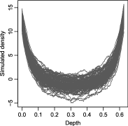
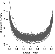
(a)	(b)

Figure 5: Simulated profiles. The profiles in panel (a) are generated from the Gaussian process, while those in panel (b) follow a scaled $t_{3}$ process.

profiles $Y_{i}(x)$ under the two error distributions. We see that the profiles generated from the $t$ process have more turbulence than those generated from the Gaussian process.

Screening

We next construct the control charts using the proposed method. When estimating the reference and deviation functions, we choose the optimal CV bandwidths $b_{n}$ and $h_{n}$ as 0.004 and 0.007, respectively, for the Gaussian $e(x)$, and 0.01 and 0.007, respectively, for the $t_{3}$ distributed $e(t)$. The three control limits are obtained assuming the overall significance level of 0.05 following equation (11). To investigate the screening power of the proposed control charts for the two sets of profiles above, we generate another 100 profiles from the true model (12) and from each of the following two “wrong” models:

$$\mbox{Model (a)\quad}Y_{i}(x) = a_{i}+\pi(x)^{\top}{\bolds{\alpha}}+A\sin(10\pi x)+e_{i}(x),$$

$$\mbox{Model (b)\quad}Y_{i}(x) = a_{i}+\pi(x)^{\top}{\bolds{\alpha}}+B\phi(x-0.3)/0.005+e_{i}(x),$$

where $a_{i}$ and $e_{i}(x)$ follow the same error process in the true model, either the Gaussian or the $t_{3}$ distribution, and $\phi(\cdot)$ is the density function of a standard normal. Model (a) distorts the shape of the profile by adding a sine curve with the coefficient $A$ determining its amplitude, while model (b) introduces local “spiky” noise to the profile. The noise level is determined by the coefficient $B$. We consider the coefficients $A$ = 0.75, 1 and 1.25 for model (a), and $B$ = 0.02, 0.03 and 0.04 for model (b), representing smaller to larger contamination scales. Figure 6 displays the simulated profiles from

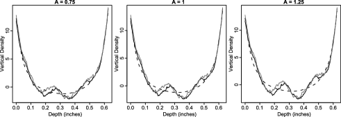
(a)

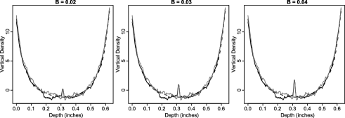
(b)

Figure 6: Simulated density profiles from the misspecified models (a) and (b). The dotted curve is the true reference profile, the solid black curves are simulated paths from the $t_{3}$ process, and the solid dark gray curves are those generated from the Gaussian process.

the two misspecified models with the Gaussian and $t_{3}$ processes, respectively. As we can see in Figure 6, when the coefficients $A$ and $B$ increase, the severity of the noise also increases. We then apply the proposed screening procedure, with the resulting proportions of successful identification presented in Table 1. When the profiles are generated from the true model, the false discovery rates are 0.05 ($\pm 0.02$) and 0.08 ($\pm 0.02$), respectively. They are close to their nominal level 0.05. For misspecified models, the screening power increases with the amplitude of the noise. In both cases, we have decent power to detect moderate to larger profile deviations. When the error $e(t)$ follows the $t_{3}$ distribution, the profiles fluctuate more, and, consequently, the screening power is lower than that of the Gaussian process.

4 Discussion

This paper proposes to screen the shape of the profiles using a nonparametric location-scale $L$-1 model. The basic idea is to estimate a reference profile curve, based on which we can rank the differences of individual profiles from the reference profile. The nonparametric components of the proposed

Table 1: The percent of the profiles that exceed the control limits. Under the true model, type I error is reported. Under models (a) and (b), the detection rate is reported

		Model (a)			Model (b)
	True model	$\bolds{A=0.75}$	$\bolds{A=1.00}$	$\bolds{A=1.25}$	$\bolds{B=0.02}$	$\bolds{B=0.03}$	$\bolds{B=0.04}$
Gaussian $e(t)$	5%	45%	80%	098%	36%	82%	100%
$t_{3}$ distributed $e(t)$	8%	21%	62%	100%	12%	44%	095%

model provide sufficient flexibility to capture the shape of the profiles. In addition, as inherited from $L$-1 regression, we do not assume any specific distributions for the profiles, and the resulting estimates are fairly robust against the heavy-tail distributions and data contamination.

$L$-1 versus $L$-2 screenings

The proposed screening procedure relies on $L$-1 regression. However, it remains valid if one replaces $L$-1 regression with $L$-2 regression (least-squares regression), which is more commonly used for control charts. Specifically, to achieve $L$-2 screening, we redefine $\xi_{i}$ in model (1) as the conditional mean of the $i$th profile, and define $\mu(x)$ and $s(x)$, respectively, as the conditional mean and standard deviation functions of $Y_{i}(x)-\delta_{i}$. The centers $\delta_{i}$ can be estimated by the sample mean of the $i$th profile, and the functions $\mu(x)$ and $s(x)$ can be estimated using kernel smoothing to replace the absolute value functions in (2) and (4) with square functions. Consequently, we define the deviation score $d_{i}$ by the standardized $\delta_{i}$, using its mean and standard deviation, and keep the deviation scores $T_{1}$ and $T_{2}$ in the same form, except that $\mu(x)$ and $s(x)$ are now the conditional mean and standard deviation functions. The $L$-2 screening could be more efficient and effective for normative profiles, but the $L$-1 screening is known to be more robust if the Phase I profiles contain potential outliers. Practitioners can choose according to their specific needs.

Profile monitoring is a relatively new area, but it is growing rapidly, as indicated by increasing numbers of practical applications. The proposed methods are shown to be favorable when applied to the previously analyzed VDP data. They can be further generalized to reach a wider range of applications. First of all, we rank the shape deviation of an individual profile from the reference profile based on its largest residual and cumulative residuals. The asymptotic distributions of the resulting deviation scores are studied. Depending on the application, alternative deviation scores can be used. For example, instead of the largest residual, we can use the 90th percentile of the residuals. The properties of other deviation scores would be of research interest. Second, the proposed charts consist of three metrics, monitoring deviations in location, shape and local disturbances, respectively. If one type of deviation is of major concern, one could focus on one metric (more targeted screening) to achieve better screening power. Third, in some applications, the data may exhibit specific features. Incorporating these special features into the estimation can further improve efficiency. For example, suppose that the VDP profile is assumed to be symmetric around the midpoint $c_{x}$. If we assume that the location function $\mu(x)$ is a smooth differentiable function, a more efficient way to estimate it is to regress $y_{i,j}$ over the transformed location $x_{i,j}^{*}=|x_{i,j}-c_{x}|$, that is, estimate the conditional median function $\mbox{median}(y_{i,j}|x_{i,j}^{*})=g(x_{i,j}^{*})$ with the constraint $g^{\prime}(0)=0$. Consequently, the location function $\mu(x)$ equals $g(|x-c_{x}|)$. Fourth, we assume in the proposed model that the errors are in a stationary random sequence. The developed theories can be further generalized to incorporate more general error sequences. For example, $e_{i,j}$ could be a linear combination of $k$ stationary error sequences. Fifth, the control limits are estimated from data, and hence subject to certain estimation errors [Jensen et al. (2006)]. When there are insufficient Phase I profiles, some corrections may be needed to ensure good properties of the proposed control charts. Finally, note that we use Phase I profiles to generate the reference distributions of the shape deviation scores. This approach implicitly assumes that there are a sufficient number of Phase I profiles that have been measured at similar locations as the profile to be screened. In the case of sparse profile data with irregular spacing, we may not have sufficient Phase I profiles to ensure a stable estimation of the screening thresholds. Further research is needed to deal with such sparse profile data.

Appendix: Conditions of Theorem 1

Recall that, for a given $i$, $\{e_{i,j}\}_{1\leq j\leq m_{i}}$ is the error process of the $i$th profile. We assume that there exist an independent process $\{e_{\ell}\}_{\ell\in\mathbb{Z}}$, such that the $i$th error profile $\{e_{i,j}\}_{1\leq j\leq m_{i}}$ can be viewed as one realization of the process $\{e_{\ell}\}_{1\leq\ell\leq m_{i}}$. We assume that $\{e_{\ell}\}_{\ell\in\mathbb{Z}}$ has the representation

$$e_{\ell}=G(\varepsilon_{\ell},\varepsilon_{\ell\pm 1},\varepsilon_{\ell\pm 2},\ldots),$$ (14)

where $\varepsilon_{\ell},\ell\in\mathbb{Z}$, are i.i.d. random vectors, and $G$ is a measurable function such that $e_{\ell}$ is well defined. The representation (14) can be viewed as an input-output system with $(\varepsilon_{\ell},\varepsilon_{\ell\pm 1},\varepsilon_{\ell\pm 2},\ldots)$, $G$ and $e_{\ell}$ being the input, transform or filter, and output, respectively. This representation allows for noncausal models, and is hence particularly useful for our applications, which do not have a time structure.

For $q>0$ and a random variable $e$ we denote by $\|e\|_{q}=[\mathbb{E}(|e|^{q})]^{1/q}$ the $L_{q}$ norm. We further assume the following:

Condition 1 ((Dependence condition)).

Let $e_{0}$ be as in (14), and $(\varepsilon^{\prime}_{\ell})_{\ell\in\mathbb{Z}}$ be an i.i.d. copy of $(\varepsilon_{\ell})_{\ell\in\mathbb{Z}}$. There exist $q>0$ and $\rho\in(0,1)$ such that for all $k\in\mathbb{N}$,

$$\|e_{0}-e_{0}(k)\|_{q}=O(\rho^{k})\hskip 80.0pt$$ (16)

$$\eqntext{\mbox{where }e_{0}(k)=G\bigl{(}\varepsilon_{0},\varepsilon_{\pm 1},\ldots,\varepsilon_{\pm k},\varepsilon^{\prime}_{\pm(k+1)},\varepsilon^{\prime}_{\pm(k+2)},\ldots\bigr{)}.}$$

In (16), $e_{0}(k)$ can be viewed as a coupling process of $e_{0}$ with $\varepsilon_{r}$ being coupled by the i.i.d. copy $\varepsilon^{\prime}_{r}$ for $|r|\geq(k+1)$, while keeping the nearest $2k+1$ innovations $\varepsilon_{r}$ with $|r|\leq k$. In particular, if $e_{0}$ does not depend on $(\varepsilon_{r})_{|r|\geq(k+1)}$, then $e_{0}(k)=e_{0}$. Thus, $\|e_{0}-e_{0}(k)\|_{q}$ can be viewed as the impact of $(\varepsilon_{r})_{|r|\geq(k+1)}$ on $e_{0}$. Intuitively, it is reasonable to expect that measurements sufficiently far away would have negligible impact. In particular, condition (16) states that the impact decays exponentially as the location space $k$ increases. As shown in Lemma 1 of Wei, Zhao and Lin (2011), (16) implies that the correlation between $e_{0}$ and $e_{\ell}$ decays exponentially as $\ell$ increases.

Condition 2 ((Location condition)).

The set of measurement locations $\{x_{i,j},1\leq j\leq m_{i},1\leq i\leq n\}$ is asymptotically uniformly dense in $[a,b]$. Specifically, let $a=\tilde{x}_{0}<\tilde{x}_{1}<\cdots<\tilde{x}_{N_{n}}<\tilde{x}_{N_{n}+1}=b$ be the ordered locations, where $N_{n}=m_{1}+\cdots+m_{n}$ is the total number of measurements. We assume that ${\max_{0\leq k\leq N_{n}}}|\tilde{x}_{k+1}-\tilde{x}_{k}-\frac{b-a}{N_{n}}|=O(N^{-2}_{n})$.

Condition 3 ((Kernel condition)).

Let ${\mathcal{K}}_{\omega},\omega>0$, be the set of kernels which are bounded, symmetric, and have bounded support $[-\omega,\omega]$ with bounded derivative. Let $\varphi_{K}=\int_{\mathbb{R}}K^{2}(u)\,du$ and $\psi_{K}=\int_{\mathbb{R}}u^{2}K(u)\,du/2,\mbox{$K\in{\mathcal{K}}_{\omega}$}$. The kernel $K\in{\mathcal{K}}_{\omega}$.

Condition 4 ((Smoothness condition)).

Denote by $F_{e}$ and $f_{e}=F^{\prime}_{e}$, respectively, the distribution and density functions of $e_{0}$ in (14). Assume $\mu,\allowbreak s\in{\mathcal{C}}^{4}([a,b]),\inf_{s\in[a,b]}s(x)>0,f_{e}\in{\mathcal{C}}^{4}(\mathbb{R}),f_{e}(0)>0,f_{e}(1)+f_{e}(-1)>0$. Here ${\mathcal{C}}^{4}(S)$ is the set of 4th order continuously differentiable functions on set $S$.

Condition 2 says that the pooled locations of measurements should be reasonably uniformly dense, even though each single profile may only contain sparse measurements. The remaining two conditions are also fairly general, and commonly assumed in kernel smoothing. Under Conditions 1–4 and $\Xi_{n}\to 0$ (see Theorem 1 for definition), the location and scale function estimates, $\tilde{\mu}_{b_{n}}$ and $\tilde{s}_{h_{n}}$, are uniformly consistent.

[id=suppA] Proof of Theorem 1 [doi]10.1214/11-AOAS501SUPP [url]http://lib.stat.cmu.edu/aoas/501/supplement.pdf .pdf The technical proof of Theorem 1 is provided in the supplementary material.

References

- Chicken, Pignatiello and Simpson (2009) {barticle}[auto:STB—2012/01/05—16:28:07] \bauthor\bsnmChicken, \bfnmE.\binitsE., \bauthor\bsnmPignatiello, \bfnmJ. J.\binitsJ. J. Jr. and \bauthor\bsnmSimpson, \bfnmJ.\binitsJ. (\byear2009). \btitleStatistical process monitoring of nonlinear profiles using wavelets. \bjournalJournal of Quality Technology \bvolume41 \bpages198–212. \bptokimsref \endbibitem
- Ding, Zeng and Zhou (2006) {barticle}[auto:STB—2012/01/05—16:28:07] \bauthor\bsnmDing, \bfnmY.\binitsY., \bauthor\bsnmZeng, \bfnmL.\binitsL. and \bauthor\bsnmZhou, \bfnmS.\binitsS. (\byear2006). \btitlePhase I analysis for monitoring nonlinear profiles in manufacturing processes. \bjournalJournal of Quality Technology \bvolume38 \bpages199–216. \bptokimsref \endbibitem
- Fan and Gijbels (1996) {bbook}[mr] \bauthor\bsnmFan, \bfnmJ.\binitsJ. and \bauthor\bsnmGijbels, \bfnmI.\binitsI. (\byear1996). \btitleLocal Polynomial Modelling and Its Applications. \bseriesMonographs on Statistics and Applied Probability \bvolume66. \bpublisherChapman and Hall, \baddressLondon. \bidmr=1383587 \bptokimsref \endbibitem
- Fan and Yao (2003) {bbook}[mr] \bauthor\bsnmFan, \bfnmJianqing\binitsJ. and \bauthor\bsnmYao, \bfnmQiwei\binitsQ. (\byear2003). \btitleNonlinear Time Series: Nonparametric and Parametric Methods. \bpublisherSpringer, \baddressNew York. \biddoi=10.1007/b97702, mr=1964455 \bptokimsref \endbibitem
- Galambos (1987) {bbook}[mr] \bauthor\bsnmGalambos, \bfnmJanos\binitsJ. (\byear1987). \btitleThe Asymptotic Theory of Extreme Order Statistics, \bedition2nd ed. \bpublisherKrieger, \baddressMelbourne, FL. \bidmr=0936631 \bptokimsref \endbibitem
- Gardner et al. (1997) {barticle}[mr] \bauthor\bsnmGardner, \bfnmMartha Maples\binitsM. M., \bauthor\bsnmLu, \bfnmJ. C.\binitsJ. C., \bauthor\bsnmGyurcsik, \bfnmR. S.\binitsR. S., \bauthor\bsnmWortman, \bfnmJ. J.\binitsJ. J., \bauthor\bsnmHornung, \bfnmB. E.\binitsB. E., \bauthor\bsnmHeinisch, \bfnmH. H.\binitsH. H., \bauthor\bsnmRying, \bfnmE. A.\binitsE. A., \bauthor\bsnmRao, \bfnmS.\binitsS., \bauthor\bsnmDavis, \bfnmJ. C.\binitsJ. C. and \bauthor\bsnmMozumder, \bfnmP. K.\binitsP. K. (\byear1997). \btitleEquipment fault detection using spatial signatures. \bjournalIEEE Transactions on Components, Packaging, and Manufacturing Technology—Part C \bvolume20 \bpages295–304. \bptokimsref \endbibitem
- He (1997) {barticle}[auto:STB—2012/01/05—16:28:07] \bauthor\bsnmHe, \bfnmX.\binitsX. (\byear1997). \btitleQuantile curves without crossing. \bjournalAmer. Statist. \bvolume51 \bpages186–192. \bptokimsref \endbibitem
- Jensen, Birch and Woodall (2008) {barticle}[auto:STB—2012/01/05—16:28:07] \bauthor\bsnmJensen, \bfnmW. A.\binitsW. A., \bauthor\bsnmBirch, \bfnmJ. B.\binitsJ. B. and \bauthor\bsnmWoodall, \bfnmW. H.\binitsW. H. (\byear2008). \btitleMonitoring correlation within linear profiles using mixed models. \bjournalJournal of Quality Technology \bvolume40 \bpages167–183. \bptokimsref \endbibitem
- Jensen and Birch (2009) {barticle}[auto:STB—2012/01/05—16:28:07] \bauthor\bsnmJensen, \bfnmW. A.\binitsW. A. and \bauthor\bsnmBirch, \bfnmJ. B.\binitsJ. B. (\byear2009). \btitleProfile monitoring via nonlinear mixed models. \bjournalJournal of Quality Technology \bvolume41 \bpages18–34. \bptokimsref \endbibitem
- Jensen et al. (2006) {barticle}[auto:STB—2012/01/05—16:28:07] \bauthor\bsnmJensen, \bfnmW. A.\binitsW. A., \bauthor\bsnmJones-Farmer, \bfnmL. A.\binitsL. A., \bauthor\bsnmChamp, \bfnmC. W.\binitsC. W. and \bauthor\bsnmWoodall, \bfnmW. H.\binitsW. H. (\byear2006). \btitleEffects of parameter estimation on control chart properties: A literature review. \bjournalJournal of Quality Technology \bvolume38 \bpages349–364. \bptokimsref \endbibitem
- Jeong, Lu and Wang (2006) {barticle}[auto:STB—2012/01/05—16:28:07] \bauthor\bsnmJeong, \bfnmM. K.\binitsM. K., \bauthor\bsnmLu, \bfnmJ. C.\binitsJ. C. and \bauthor\bsnmWang, \bfnmN.\binitsN. (\byear2006). \btitleWavelet based SPC procedure for complicated functional data. \bjournalInternational Journal of Production Research \bvolume44 \bpages729–744. \bptokimsref \endbibitem
- Kang and Albin (2000) {barticle}[auto:STB—2012/01/05—16:28:07] \bauthor\bsnmKang, \bfnmL.\binitsL. and \bauthor\bsnmAlbin, \bfnmS. L.\binitsS. L. (\byear2000). \btitleOn-line monitoring when the process yields a linear profile. \bjournalJournal of Quality Technology \bvolume32 \bpages418–426. \bptokimsref \endbibitem
- Kim, Mahmoud and Woodall (2003) {barticle}[auto:STB—2012/01/05—16:28:07] \bauthor\bsnmKim, \bfnmK.\binitsK., \bauthor\bsnmMahmoud, \bfnmM. A.\binitsM. A. and \bauthor\bsnmWoodall, \bfnmW. H.\binitsW. H. (\byear2003). \btitleOn the monitoring of linear profiles. \bjournalJournal of Quality Technology \bvolume35 \bpages317–328. \bptokimsref \endbibitem
- Koenker (2005) {bbook}[mr] \bauthor\bsnmKoenker, \bfnmRoger\binitsR. (\byear2005). \btitleQuantile Regression. \bseriesEconometric Society Monographs \bvolume38. \bpublisherCambridge Univ. Press, \baddressCambridge. \biddoi=10.1017/CBO9780511754098, mr=2268657 \bptokimsref \endbibitem
- Li and Racine (2007) {bbook}[mr] \bauthor\bsnmLi, \bfnmQi\binitsQ. and \bauthor\bsnmRacine, \bfnmJeffrey Scott\binitsJ. S. (\byear2007). \btitleNonparametric Econometrics. \bpublisherPrinceton Univ. Press, \baddressPrinceton, NJ. \bidmr=2283034 \bptokimsref \endbibitem
- Mahmoud et al. (2007) {barticle}[auto:STB—2012/01/05—16:28:07] \bauthor\bsnmMahmoud, \bfnmM. A.\binitsM. A., \bauthor\bsnmParker, \bfnmP. A.\binitsP. A., \bauthor\bsnmWoodall, \bfnmW. H.\binitsW. H. and \bauthor\bsnmHawkins, \bfnmD. M.\binitsD. M. (\byear2007). \btitleA change point method for linear profile data. \bjournalQuality and Reliability Engineering International \bvolume23 \bpages247–268. \bptokimsref \endbibitem
- Opsomer, Wang and Yang (2001) {barticle}[mr] \bauthor\bsnmOpsomer, \bfnmJean\binitsJ., \bauthor\bsnmWang, \bfnmYuedong\binitsY. and \bauthor\bsnmYang, \bfnmYuhong\binitsY. (\byear2001). \btitleNonparametric regression with correlated errors. \bjournalStatist. Sci. \bvolume16 \bpages134–153. \biddoi=10.1214/ss/1009213287, issn=0883-4237, mr=1861070 \bptokimsref \endbibitem
- Qiu, Zou and Wang (2010) {barticle}[mr] \bauthor\bsnmQiu, \bfnmP.\binitsP., \bauthor\bsnmZou, \bfnmC.\binitsC. and \bauthor\bsnmWang, \bfnmZ.\binitsZ. (\byear2010). \btitleNonparametric profile monitoring by mixed effects modeling. \bjournalTechnometrics \bvolume52 \bpages283–285. \bptokimsref \endbibitem
- Reis and Saraiva (2006) {barticle}[mr] \bauthor\bsnmReis, \bfnmMarco S.\binitsM. S. and \bauthor\bsnmSaraiva, \bfnmPedro M.\binitsP. M. (\byear2006). \btitleMultiscale statistical process control of paper surface profiles. \bjournalQual. Technol. Quant. Manag. \bvolume3 \bpages263–281. \bidissn=1684-3703, mr=2312643 \bptokimsref \endbibitem
- Shiau et al. (2009) {barticle}[mr] \bauthor\bsnmShiau, \bfnmJyh-Jen Horng\binitsJ.-J. H., \bauthor\bsnmHuang, \bfnmHsiang-Ling\binitsH.-L., \bauthor\bsnmLin, \bfnmShuo-Hui\binitsS.-H. and \bauthor\bsnmTsai, \bfnmMing-Ye\binitsM.-Y. (\byear2009). \btitleMonitoring nonlinear profiles with random effects by nonparametric regression. \bjournalComm. Statist. Theory Methods \bvolume38 \bpages1664–1679. \biddoi=10.1080/03610920802702535, issn=0361-0926, mr=2538166 \bptokimsref \endbibitem
- Walker and Wright (2002) {barticle}[auto:STB—2012/01/05—16:28:07] \bauthor\bsnmWalker, \bfnmE.\binitsE. and \bauthor\bsnmWright, \bfnmS. P.\binitsS. P. (\byear2002). \btitleComparing curves using additive models. \bjournalJournal of Quality Technology \bvolume34 \bpages118–129. \bptokimsref \endbibitem
- Wei, Zhao and Lin (2011) {bmisc}[auto:STB—2012/01/05—16:28:07] \bauthor\bsnmWei, \bfnmY.\binitsY., \bauthor\bsnmZhao, \bfnmZ.\binitsZ. and \bauthor\bsnmLin, \bfnmD. K. J.\binitsD. K. J. (\byear2011). \bhowpublishedSupplement to “Profile control charts based on nonparametric -1 regression methods.” DOI:10.1214/11-AOAS501SUPP. \bptokimsref \endbibitem