Phase diagrams of a p-wave superconductor inside a mesoscopic disc-shaped sample

Abstract

We study the finite-size and boundary effects on a time-reversal-symmetry breaking p-wave superconducting state in a mesoscopic disc geometry using Ginzburg-Landau theory. We show that, for a large parameter range, the system exhibits multiple phase transitions. The superconducting transition from the normal state can also be reentrant as a function of external magnetic field.

Studies of Fermi superfluids and superconductors with multi-component order parameters have drawn much attention over the last few decades. A well-established example is spin-triplet p-wave superfluid ³He He3 , the order parameter of which is a complex $3\times 3$ matrix instead of a single component scalar as in the case of s-wave superconductors. Many unusual behaviors of this superfluid are known, in particular ”textures”, where the order parameter varies in space in a non-trivial way due to external fields, flows, or confining walls. There have also been intense studies of superconductors that are believed also to possess multi-component order parameters, for example, UPt₃ UPt3 and Sr₂RuO₄ SrRuO . While the precise order parameters in both cases are still controversial, many believe that both these two superconductor have order parameters which break time-reversal symmetry. Broken time reversal symmetry necessarily requires a multi-component order parameter. A single component order parameter, though it can belong to a non-trivial one-dimensional representation, cannot break time-reversal symmetry in the sense that its complex conjugate differs from the original one only via a gauge transformation. A superconductor with broken time reversal symmetry can have exotic properties, such as circular dichroism and birefringence (Kerr rotation) Kapitulnik09 , internal magnetic fields Muzikar and surface currents surfacecurrent , to name a few. Experiments claimed to support broken time reversal symmetry have been reported both for UPt₃ Luke93 ; Strand and Sr₂RuO₄ Luke98 ; Kidwingira , though negative results are also in the literature Kambara96 ; Hicks10 . Other aspects of intense recent interest are half-quantum vortices Budakian11 arising from the spin degrees of freedom, and Majorana vortex bound states M , which would be possible if the order parameter is a p-wave with the form $p_{x}+ip_{y}$, which is the case proposed for Sr₂RuO₄.

In this paper, we study a two-component superconductor in a confined geometry. Our motivations are several folded. First, as mentioned, in the context of ³He, a confining geometry can induce a non-trivial texture. A surface is necessarily a strong breaker of rotational invariance, and hence its effect on the order parameter depends on the relative orientation between the two. The energetically most favorable configuration therefore does not necessarily correspond to simply taking the uniform bulk order parameter and suppressing its magnitude near the surface. Second, for a multi-component order parameter, or more precisely an order parameter that belongs to a multi-dimensional representation, the different components possess the same transition temperature $T_{c}^{0}$ in the bulk in the absence of external perturbations (by definition). However, external perturbations can split the degeneracies, resulting in multiple phase transitions. This has been discussed in the context of thin-films of ³He-B Kawasaki04 , as well as for UPt₃ under the influence of the underlying anti-ferromagnetic order UPt3 . There have also been many recent experimental studies of mesoscopic superconductors, s meso-s , p Cai , and d wave meso-d , including some interesting theoretical predications for the latter, e.g. meso-d-t , but the physics associated with the multi-component nature of the order parameter is less explored in the literature.

We shall consider a thin circular disc of radius $R$ lying in the x-y plane. Variation of the order parameter along z, as well as the magnetic field generated by the supercurrent of the sample, will be ignored. We shall study a superconductor with a two-component order parameter. The two components $\eta_{x,y}$ are supposed to transform as a vector under rotations within the x-y plane. We shall study how the order parameter varies over the disc. For definiteness, $\eta_{x,y}$ are taken to be the two in-plane components of the orbital part of the p-wave order parameter, that is, the momentum dependence is $\eta_{x}p_{x}+\eta_{y}p_{y}$. However, we expect that many of our findings should be common to other superconductors with multi-component order parameter. This point will be discussed again below. Recently, a group Huo11 has studied theoretically this same system using Bogoliubov-deGennes equations. Their results however differ significantly from ours. A comparison will be given later.

We shall employ Ginzburg-Landau (GL) theory, but as we shall argue later, our conclusions are more general. The GL free energy density (per unit area) $\mathcal{F}$ consists of several contributions. The bulk contribution, $\mathcal{F}_{b}$, can be written as

$$\mathcal{F}_{b}=\alpha(\vec{\eta}^{*}\cdot\vec{\eta})+\beta_{1}(\vec{\eta}^{*}\cdot\vec{\eta})^{2}+\beta_{2}|\vec{\eta}\cdot\vec{\eta}|^{2},$$ (1)

where $\alpha=\alpha^{\prime}(t-1)$ with $\alpha^{\prime}>0$, $t\equiv{}T/T_{c}^{0}$ is the ratio of the temperature $T$ relative to the bulk transition temperature $T_{c}^{0}$, $\vec{\eta}=\eta_{x}\hat{x}+\eta_{y}\hat{y}$, which we would often denoted as $(\eta_{x},\eta_{y})$. Stability requires $\beta_{1}>0$, $\beta_{1}>-\beta_{2}$. We shall take $\beta_{2}>0$, so that for the bulk the equilibrium order parameter below $T_{c}^{0}$ has the form $\vec{\eta}=\Psi(1,\pm{}i)$, so that it has broken time-reversal symmetry, with $|\Psi|=\frac{1}{2}(\frac{\alpha^{\prime}}{\beta_{1}})^{1/2}$.

In the presence of gradients, there is an additional contribution to $\mathcal{F}$ given by

$$\mathcal{F}_{g}=K_{1}(D_{j}\eta_{l})(D_{j}\eta_{l})^{*}+K_{2}(D_{j}\eta_{j})(D_{l}\eta_{l})^{*}+K_{3}(D_{j}\eta_{l})(D_{l}\eta_{j})^{*},$$ (2)

where $D_{j}\equiv\partial_{j}+\frac{2ie}{c}A_{j}$ is the gauge invariant derivative. $\vec{A}$ is the vector potential, and the electron charge is $-e$. Repeated indices $j,l$ are summed over $x,y$ in eq.(2). In writing down eq.(1) and (2), we have ignored crystal anisotropies for simplicity, but we do not expect significant qualitative change in our predictions below. The more general forms can be found in, e.g., VG ; Sigrist . Stability requires $K_{1}>0$, $K_{123}\equiv{}K_{1}+K_{2}+K_{3}>0$. If we take $\eta_{x,y}$ to represent the two in-plane orbital components of a pure p-wave order parameter, assume that the Fermi surface is isotropic in the plane, then, within weak-coupling theory, $\beta_{2}/\beta_{1}=1/2$, and $K_{1}=K_{2}=K_{3}$ (the later holds up to particle-hole symmetric terms) He3 ; UPt3 , but we shall treat these coefficients as general parameters.

We shall limit ourselves to solutions which are cylindrically symmetric, up to an overall gauge transformation. To this end, it is convenient to introduce the cylindrical coordinates $(r,\phi)$ for space where $\phi$ is the angle between $\vec{r}$ and $\hat{x}$, and define $\eta_{\pm}=\eta_{x}\pm{}i\eta_{y}$. The bulk minimum energy solutions thus have $\eta_{-}=0$, $\eta_{+}\neq 0$, or vice versa. $\eta_{\pm}$ can be expanded as $\eta_{+}=\sum_{n}C^{(n)}_{+}(r)e^{in\phi}$, $\eta_{-}=\sum_{n}C^{(n)}_{-}(r)e^{i(n-2)\phi}$, where $n$ is integer and an extra $-2$ is introduced in the $\eta_{-}$ formula for convenience below. We have $\vec{\eta}\cdot\hat{r}=\frac{1}{2}\sum_{n}(C^{(n)}_{+}(r)+C^{(n)}_{-}(r))e^{i(n-1)\phi}$ and $\vec{\eta}\cdot\hat{\phi}=-i\frac{1}{2}\sum_{n}(C^{(n)}_{+}(r)-C^{(n)}_{-}(r))e^{i(n-1)\phi}$. For solutions that are cylindrical symmetric up to a gauge transformation, only $C_{\pm}^{(n)}$ for one particular $n$ can be finite. Therefore different solutions are classified by $n$. In these cases, $C_{\pm}^{(n)}$ can be chosen real without loss in generality.

We shall first assume that the surface at $r=R$ is smooth. If the order parameter $\vec{\eta}$ represents the momentum part of the pairing wavefunction, the component perpendicular to the surface should vanish AGD , thus

$$\vec{\eta}\cdot\hat{r}=0\qquad(r=R),$$ (3)

that is,

$$C^{(n)}_{+}+C^{(n)}_{-}=0\qquad(r=R).$$ (4)

The parallel component $\eta_{\|}\equiv\eta\cdot\hat{\phi}$ should have vanishing gradient perpendicular to a planar surface AGD . At a surface with a finite curvature, it should satisfy BF

$$K_{1}\frac{\partial}{\partial r}\eta_{\|}=\frac{K_{3}}{R}\eta_{\|}\qquad(r=R),$$ (5)

hence

$$K_{1}\frac{\partial}{\partial r}(C^{(n)}_{+}-C^{(n)}_{-})=\frac{K_{3}}{R}(C^{(n)}_{+}-C^{(n)}_{-})\qquad(r=R).$$ (6)

The differential equations satisfied by $C_{\pm}^{(n)}(r)$ can be found by simple variation, noting that the total free energy is $F=2\pi\int_{0}^{R}drr(\mathcal{F}_{b}+\mathcal{F}_{g})$. We remark here that the boundary conditions eq.(3-6) guarantee that there are no net surface terms proportional to the variation $\delta{}C_{\pm}^{(n)}(R)$ of the order parameters at the surface, when we integrate by parts the gradient terms. They also guarantee that the normal component of the current vanishes for arbitrary choice of order parameter profiles BF , as should be the case of impenetrable walls at $r=R$.

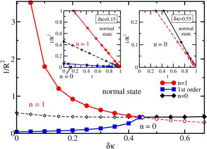
Figure 1: Zero field Phase diagram: $R$ is in unit of $\xi\equiv\sqrt{K_{123}/\alpha^{\prime}}$. The parameters are $\beta\equiv\beta_{2}/\beta_{1}=0.25$, $\kappa_{1}=1/3+\delta\kappa$, $\kappa_{2}=\kappa_{3}=1/3-\delta\kappa/2$, with $\kappa_{i}\equiv{}K_{i}/K_{123}$. Inset: R-t phase diagrams for different $\delta\kappa$’s.

First consider zero external magnetic field. It is worth having some analytic solutions before we show the numerical results. The transition temperature $t_{c}^{(1)}$ from the normal to $n=1$ state can be found analytically. The $n=1$ solutions are time-reversal symmetric, and the free energy is invariant under $C_{+}^{(1)}\longleftrightarrow\pm{}C_{-}^{(1)}$. Since the boundary conditions are also symmetric under this transformation, the equations for $C_{s}^{(1)}(r)\equiv\frac{1}{2}(C_{+}^{(1)}+C_{-}^{(1)})$ and $C_{d}^{(1)}(r)\equiv\frac{1}{2}(C_{+}^{(1)}-C_{-}^{(1)})$ decouple. One possible solution is $C_{s}^{(1)}(r)\equiv 0$ (hence $\vec{\eta}\cdot\hat{r}=0$ for all $r$), $C_{d}^{(1)}(r)\neq 0$, i.e. $C_{+}^{(1)}(r)=-C_{-}^{(1)}(r)=C^{(1)}(r)$. other After linearizing in the order parameter, it can be shown that $C^{(1)}(r)\propto{}J_{1}(\sqrt{\frac{\alpha^{\prime}(1-t_{c}^{(1)})}{K_{1}}}r)$, the Bessel function of the first kind. With eq.(6), we find the relation

$$(1-t_{c}^{(1)})=\frac{K_{1}}{\alpha^{\prime}R^{2}}a^{2}\ ,$$ (7)

where $a$ should satisfy $aJ^{\prime}_{1}(a)=\frac{K_{3}}{K_{1}}J_{1}(a)$. The critical temperature is suppressed by a factor $\propto 1/R^{2}$. Therefore, we can find the critical radius via $R_{c}=a\sqrt{K_{1}/\alpha^{\prime}}$, which is the minimum radius of the system to maintain the superconductivity with $n=1$ at zero temperature. Note that, due to eq.(7), it is more convenient to set the vertical axes of R-t phase diagram to be $1/R^{2}$, as shown in Fig.1. For this solution, we note that $a\to 0$ as $K_{3}\to K_{1}$, which means that in the weak-coupling limit the transition temperature for our disc with smooth boundary is not at all affected by the finite radius and in fact is the same as that of the bulk, hence $1/R_{c}^{2}\to\infty$. This can also be shown within the quasi-classical approximation, pf-weak , and is therefore not an artifact of the GL approximation. The second case with analytic solution is $K_{2}=K_{3}=0$. The order parameters near the critical point is $C_{+}^{(n)}=c_{n+}J_{n}(x)$ and $C_{-}^{(n)}=c_{n-}J_{n-2}(x)$. Here $x=r\sqrt{\frac{\alpha^{\prime}(1-t)}{K_{1}}}$. Using the boundary conditions (4) and (6), we can find the R-t relations for all $n$’s. We find that, in this case, the state with the highest transition temperature is $n=0$, which is degenerate with $n=2$.

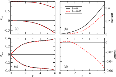
Figure 2: Order parameters (a,c) of the ground states and the corresponding current distributions (b,d) for zero (black line) and finite field (red dash). $\delta\kappa=0$, $\beta=0.25$, $R=6$. The upper plots are for $n=0$ and $t=0$; the lower plots are for $n=1$ and $t=0.7$. The order parameters are normalized to $\sqrt{\alpha^{\prime}/\beta_{1}}$, the external field $B$ is normalized as $b\equiv\frac{2eB}{c}\xi^{2}$ (roughly to the bulk upper critical field), $\delta\kappa$ and $\beta$ as defined in the caption of Fig.1.

Our obtained phase diagrams are summarized in Fig.1. Only $n=1$ and $n=0$ (or equivalently, its time-reversed partner $n=2$ with $C_{\pm}^{(0)}(r)\to{}C_{\mp}^{(2)}(r)$) can be ground states. The left inset shows the kind of R-t phase diagram for $0\leq\delta\kappa\lesssim 0.44$ nk . When the radius is smaller than a critical value, $R_{c}^{(1)}$ (y-intercept of red circle line), the system does not have any superconducting phase. If the radius is between $R_{c}^{(1)}$ and $R_{c}^{1st}$ (y-intercept of blue square line), which corresponds to the first order phase transition from $n=1$ to $n=0$ with lowering temperature, it just has the superconducting phase with $n=1$ after the second order phase transition (red circle line). For the radius larger than $R_{c}^{1st}$, we have second order phase transition from the normal state and then a first order phase transition (blue square line) to a spontaneously time-reversal-symmetric-broken superconducting state ($n=0$). In the plot, we still show where the normal state would have become unstable toward the $n=0$ state by a dashed line, which does not correspond to a real phase transition for the system since it is below the $n=1$ transition. On the other hand, if $\delta\kappa$ is large enough ($\gtrsim 0.44$) , the R-t phase diagram should be similar to the right inset of Fig.1. The system just has the possibility to be in the superconducting state with $n=0$ at low temperature (the unphysical $n=1$ instability line from the normal state is also shown as dashed). Transition lines corresponding to second order phase transition from the normal state in R-t phase diagrams are linear within GL theory. For the first order transition lines, we found numerically that they are still practically linear. The main Fig.1 displays the critical radii at zero temperature. This figure can also be regarded as a plot of the critical radii at finite temperatures after rescaling of the vertical axis by the factor $(1-t)$. The linear relations between $1/R^{2}$ and the critical temperatures are artifacts of GL theory, but we expect that the phase diagrams in Fig.1 are still qualitatively valid.

In plotting Fig.1, $\beta=0.25$ was used. The second order phase transition lines are independent of this ratio. nbeta For larger (smaller) $\beta$, the first order transition temperature (and thus the corresponding $1/R_{c}^{1st}$) is higher (lower), thus increasing (decreasing) the stability region for the $n=0$ phase. We also note that though our specific calculations are for a circular disc, the $n=0$ and $n=1$ states are distinguishable by time-reversal symmetry, and so the phase transition between them should exist even for other geometries.

To get more understanding of the phase diagram, we consider the order parameters in some detail. An example is as shown in Fig.2. Here we have chosen $\delta\kappa=0$. (We shall mostly be considering $0\leq\delta\kappa\lesssim 0.44$ for the rest of this paper). At temperatures below the first order transition temperature $t_{c}^{1st}$ ($=0.32$ here), it is a time-reversal-symmetry-broken state with $n=0$ (or $n=2$). The flat parts of the order parameters around the center reflects the characteristics of the bulk system, with $C_{+}\neq 0$ but $C_{-}\approx 0$. This is the preferred configuration at low temperatures, or equivalently, for large samples. For $t>t_{c}^{1st}$, the ground state becomes $n=1$. The vortex structure at the center is shown in Fig.2(c). The boundary condition (3) admits only the parallel component $\vec{\eta}\cdot\hat{\phi}$ near the edge of the sample, and, being at a higher temperature, the radial component $\vec{\eta}\cdot\hat{r}$ has not nucleated. This implies that we have $n=1$ transition , which is then the preferred configuration at higher temperatures or intermediate size grains. The phase diagram reflects the competition between the boundary effect, which favors $n=1$ (for $\delta\kappa<0.44$), versus the bulk, which prefers $n=0$ (or $n=2$).

At zero field, the $n=0$ ($n=2$) state has surface current surfacecurrent in $+$ ($-$) $\hat{\phi}$ direction (Fig.2(b)), hence a magnetic moment $\mathcal{M}$ along $+z$ ($-z$). The $n=1$ state, being time-reversal symmetric, has no surface current even though there are vortices at the center.

Now we consider an external magnetic field $B$ along the $+$z direction. First we consider very small fields. The degeneracies between $n=0$ and $n=2$ are lifted. $n=0$ is favored since its magnetic moment $\mathcal{M}$ is parallel to the external field. The reduction of current near the edge due to external field in Fig.2(b) is due to the Meissner effect. For the time-reversal-symmetric state, with the applied magnetic field, the system has negative current near the edge and positive current around the vortex.

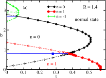
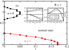
Figure 3: b-t phase diagram: $R=1.4$ and $1$, $\delta\kappa=0.15$,$\beta=0.25$. Inset: order parameter and current at $b=2.5$ and $2.9$, $t=0$.

For larger fields, the phase diagram can be modified. In this paper, we focus on discs with small radii and small magnetic field. (At larger grains or fields, cylindrical symmetry can be broken due to the possibility of vortex lattice. We ignore this possibility in this paper). An example is shown for $R=1.4$ in Fig.3(a). The $n=1$ state is always suppressed by the external field due to the kinetic energy of the Meissner current. However, for $n=0$, due to its spontaneous magnetic moment at zero field, it is first enhanced by the field, then eventually suppressed at larger fields. Hence, above a certain field, $n=0$ can become more favorable than $n=1$. The transition to the superconducting state can thus become reentrant as a function of magnetic field. At still higher fields, other $n$’s (such as $n=-1$ here) can become the ground state. For even smaller grains, the reentry of superconductivity becomes more significant. An example is shown in Fig.3(b), where superconductivity disappears completely for intermediate fields. This reentrance of superconductivity is similar to the Little-Parks effect in s-wave superconductors in multi-connected geometries lp-effect . We note that the enhancement or suppression of superconductivity by $B$ can be understood from the net magnetic moment of the grain, (hence the current, see inset of Fig.3(b)) since $\frac{\partial{}F}{\partial{}B}\propto-\mathcal{M}$.

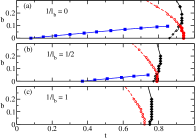
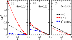
Figure 4: (a-c) Phase diagram: effect of rough boundary on the b-t phase diagram with $R=4$ and $\delta\kappa=0.15$. (d-f) Zero-field phase diagram with rough boundary for different $\delta\kappa$’s. $l_{b}=2.0$.

Recently, Huo11 studies a p-wave superconductor in a disc, solving the Bogoliubov-deGennes equation together with a weak-coupling gap equation, assuming a cylindrically symmetric Fermi surface and also a smooth boundary at $R$. Our results for $\delta\kappa=0$ should then be applicable, but are different in many ways from theirs. In zero field and some $R$, they showed a transition from the normal state to the $n=0$ state. We however found that the transition from the normal state should always be first to the time-reversal symmetric $n=1$ state, though the system can make a first order transition later to the $n=0$ state at a lower temperature for grains that are not too small (Fig.1). While both they and we found reentrance of superconductivity as function of magnetic field, our reentrance is always to a state which is connected with the one with broken time-reversal symmetry ($n=0$, $-1$, etc here), but theirs is into a state that is connected with the time-reversal symmetric one ($n=1$) in zero field (Fig.3). Also, we did not find any reentrant behavior as a function of temperature, in contrast to Huo11 .

In the above, we have assumed a smooth boundary at $r=R$. In order to mimic an imperfect boundary, we introduce the diffusive boundary term, $\mathcal{F}_{s}=K_{1}C_{d}^{2}/l_{b}$, for the free energy.Sigrist Here $C_{d}=(C_{+}-C_{-})/2$ and positive $l_{b}$ is the extrapolation length due to boundary scattering. This energy term will modify the boundary condition, eq.(6). The factor in front of the order parameter of right hand side becomes $(K_{3}/R)-(K_{1}/l_{b})$, as obtained in AGD using a more microscopic consideration. Fig.4(a-c) show the effect of rough boundary for $R=4$. The $T_{c}$ for $n=1$ is suppressed more than that for $n=0$. However, the $T_{c}^{1st}$ for the 1st order phase transition becomes larger for rough boundary. The system can be just in the superconducting state with $n=0$ for sufficiently rough boundary (as shown in Fig.4(c)). Fig.4(d-f) are the R-t phase diagrams for different $\delta\kappa$’s without external field. Comparing these phase diagrams with the insets in Fig.1, the second order transition lines have negative curvatures. The critical radius for the existence of superconductivity at $\delta\kappa=0$ becomes finite. The critical radii at zero temperature gives a phase diagram similar to Fig.1, except some shift of the curves to the left.

In conclusion, we study the phase transition of a two-component superconductor in a confined geometry. We find that, in a large order parameter space, the system would exhibit multiple phase transitions. While we have mostly been referring to a p-wave superconducting order parameter, we expect that many of the qualitative features here would remain so long as the surface affects the two components of the order parameter differently. These phase transitions can be detected by, for example, measuring the density of states via tunneling meso-s , in grains of size of order of coherence length.

This work is supported by the National Science Council of Taiwan under grant number NSC-98-2112-M-001 -019 -MY3.

References

- (1) A. J. Leggett, Rev. Mod. Phys. 47, 331 (1975); D. Vollhardt and P. Wölfle, The Superfluid Phases of Helium 3, Taylor and Francis, London (1990).
- (2) J. A. Sauls, Advances in Physics, 43, 113 (1994); Robert Joynt and Louis Taillefer, Rev. Mod. Phys. 74, 235 (2002).
- (3) A. P. MacKenzie and Y. Maeno, Rev. Mod. Phys. 75, 657 (2003); Y. Maeno, S. Kittaka, T. Nomura, S. Yonezawa, and K. Ishida, J. Phys. Soc. Jpn. 81, 011009 (2012).
- (4) A. Kapitulnik, J. Xia, E. Schemm and A. Palevski, New J. Phys. 11, 055060 (2009).
- (5) C. H. Choi and P. Muzikar, Phys. Rev. B 39, 9664 (1989).
- (6) M. Matsumoto and M. Sigrist, J. Phys. Soc. Jpn. 68, 994 (1999); 68, 3120 (E) (1999); M. Stone and R. Roy, Phys. Rev. B 69, 184511 (2004); J. A. Sauls, ibid, 84, 214509 (2011)
- (7) G. M. Luke et al, Phys. Rev. Lett. 71, 1466 (1993).
- (8) J. D. Strand, D. J. Van Harlingen, J. B. Kycia, and W. P. Halperin, Phys. Rev. Lett. 103, 197002 (2009)
- (9) G. M. Luke et al, Nature 394, 558 (1998).
- (10) F. Kidwingira, J. D. Strand, D. J. VAn Harlingen, and Y. Maeno, Science 314, 1267 (2006).
- (11) H. Kambara et al, Europhys. Lett. 36, 545 (1996).
- (12) C. W. Hicks et al, Phys. Rev. B 81, 214501 (2010).
- (13) J. Jang et al, Science 331, 186 (2011).
- (14) S. Das Sarma, C. Nayak and S. Tewari, Phys. Rev. B 73, 220502 (2006)
- (15) K. Kawasaki et al, Phys. Rev. Lett. 93, 105301 (2004).
- (16) T. Cren, L. Serrier-Garcia, F. Debontridder, and D. Roditchev, Phys. Rev. Lett. 107, 097202 (2011).
- (17) X. Cai, Y. A. Ying, N. E. Staley, Y. Xin, D. Fobes, T. Liu, Z. Q. Mao, and Y. Liu, arXiv:1202.3146.
- (18) I. Sochnikov et al, Nature Nanotechnology, 5, 516 (2010).
- (19) A. B. Vorontsov, Phys. Rev. Lett. 102, 177001 (2009).
- (20) J-W Huo, W-Q Chen, S. Raghu and F-C Zhang, arXiv:1108.2380.
- (21) G. E. Volovik and L. P. Gorkov, Sov. Phys. JETP 61, 843 (1985).
- (22) M. Sigrist and K. Ueda, Rev. Mod. Phys. 63, 239 (1991).
- (23) V. Ambegaokar, P. de Gennes and D. Rainer, Phys. Rev. A 9, 2676 (1974); 12, 345 (E) (1975).
- (24) L. J. Buchholtz and A. L. Fetter, Phys. Rev. B 15, 5225 (1977).
- (25) The other possible choice with , with boundary condition is found to be unfavorable so long as .
- (26) See Supplemental Material.
- (27) For , the superconducting transition temperature would actually be enhanced by the finite radius. We however have not pursued this peculiar situation further.
- (28) Note that this predicts that for , , the normal state first undergoes an instability into a time-reversal symmetry breaking state upon lowering of the temperature, even though that the bulk only favors a time-reversal symmetric state.
- (29) for all requires for all , which is not possible except since obey different equations. has phase winding but has (see the equations in the paragraph above eq.(3)). is possible due to time reversal symmetry (see discussion above eq.(7)).
- (30) W. A. Little and R. D. Parks, Phys. Rev. Lett. 9, 9 (1962).