LISA: Locally Interacting Sequential Adsorption

Abstract

We study a class of dynamically constructed point processes in which at every step a new point (particle) is added to the current configuration with a distribution depending on the local structure around a uniformly chosen particle. This class covers, in particular, generalised Polya urn scheme, Dubbins–Freedman random measures and cooperative sequential adsorption models studied previously. Specifically, we address models where the distribution of a newly added particle is determined by the distance to the closest particle from the chosen one. We address boundedness of the processes and convergence properties of the corresponding sample measure. We show that in general the limiting measure is random when exists and that this is the case for a wide class of almost surely bounded processes.

Keywords: sequential adsorption, stopping set, point process, random measure, Polya urn, convergence of empirical measures

AMS 2010 Subject Classification: primary 60G55; secondary 60G57, 60D05, 60F99, 82C22

1 Introduction

A model of sequentially constructed point process that inspired this paper was presented to one of the authors (SZ) by Richard W. R. Darling as a way to describe a certain population dynamics. His original model is described as follows. Start with a fixed finite configuration $X=\{x_{1},\dotsc,x_{n_{0}}\}$ of $n_{0}$ points in a plane. Call them particles. Choose one of these particles uniformly at random. This particle, say $\xi$, is thought of as a ‘parent’ of a new particle that will be added to the current configuration according to the following rule. Consider $k$ closest to $\xi$ particles $x_{1}(\xi),\dotsc,x_{k}(\xi)$, where $k\geq 3$ is a parameter of the model, and fit a 2-variate Normal distribution centred in $\xi$ to these. Let $\widehat{V}$ be the corresponding estimate of the covariance matrix. Then sample a new particle from this estimated law: $x_{n_{0}+1}\sim\mathcal{N}(\xi,\widehat{V})$. Once this is done, we have a configuration of $n_{0}+1$ particles and we repeat the procedure again: choose randomly a particle among all $n_{0}+1$ particles now present, estimate the Normal law from the closest to it $k$ particles and add a new particle sampled from this law, etc.

A realisation of the model based on 20 initial particles after 10 thousand steps is shown in the upper-left plot in Figure 1.

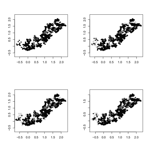
Figure 1: Sequence of 10, 20, 30 and 40 thousand generated particles. Newly added ten thousand particles are in dark, previously existing – in grey (partially covered), initial particles are contoured void circles.

One can note the following characteristic features of the construction. Since the parent particle is chosen uniformly, there is a greater chance that this parent will be chosen in the area densely populated by the particles. Moreover, in these dense areas the distance between the particles tends to be small, so the newly added particle also tends to lie close to the parent point. So as the construction progresses, it tends to reinforce the dense areas of particles which kind of ‘adsorb’ new particles. This is clearly seen in Figure 1, where the configuration is shown after 10, 20, 30 and 40 thousand steps. Each of newly added 10 thousand particles are shown in dark emphasising their trend to follow higher density areas of the previously existing (grey) points. Note that although the configuration of existing particles plays a crucial role in the construction, only $k$ closest particles to the chosen one actually contribute to the distribution of the added point. In this sense the interaction is local, hence the name we have chosen for this process: Locally Interacting Sequential Adsorption or LISA, for short.

Another feature concerns the geometry of the cloud of particles. When the parent particle is chosen inside a circular cloud, its closest neighbours tend to be homogeneously spread around it. This produces more or less isotropic Normal density for a new point wich adds to a round cloud making it even more isotropic. In contrast, when a boundary particle is chosen as a parent or when it lies in a stretched cloud, the density will also be skewed in the corresponding direction. So in the long run round clouds tend to stay round, but time to time ‘shootouts’ from their boundary happen which then tend to produce filamentary arrangements. It also happens due to randomness that even if a parent in such a filament is chosen, it can still produce a particle well outside the main direction, and this would then become a centre of another circular cloud.

There is a range of questions arising immediately: will the particles be always confined to a bounded region or will the diameter of the cloud will increase indefinitely? Will eventually particles be present in any compact set of a positive area or will there be gaps never filled by the process? If we supply all $n$ the particles present at the current step with masses $1/n$ we get a probability sample measure $\nu_{n}$. Is there a limit in appropriate sense of the sequence of these measures? Is this limit measure when exists random or is it non-random? And what about finer properties of this limiting measure, like the Hausdorff dimension of its support?

Surely, the two-variate Normal distribution is just one of possible choices of the distribution governing addition of a new point. And all the above questions can be asked for any other distribution: for instance, to provoke shootouts one would try some heavy-tailed distribution for the distance from its centre. We, however, want to keep the main essence of the local interaction of the model above requiring that the new particle distribution scales appropriately when the configuration becomes denser. This will bring us to the notion of a stopping set described in details in the next section.

The structure of the paper is the following. In the next Section 2 we fix the notation used throughout and give formal description of the class of locally interacting sequential processes we are dealing with, the Darling’s model being one particular case of these. Other cases include such seemingly different models as Dirichlet measures, Dubbins-Freedman’s random distribution functions and cooperative sequential adsorption. Section 3 demonstrates on a simple example that the limiting distribution of particles, if exists, is generally a random measure, this particular example leads to Dubbins-Freedman construction of a random distribution function. Section 4 addresses boundedness issue and show that under rather mild conditions the cloud of points has almost surely finite diameter. Finally, Section 5 studies convergence of sample measures and shows that in models with an a. s. finite diameter such a limiting measure exists in a weak sense almost surely. LISA processes constitute a very large class of models with different properties, so we conclude by outlining extensions, relations to other models and open problems which are abound.

2 Preliminaries and Model Description

In order to define a locally interacting sequential adsorption process, we need a few components. First, the phase space $W$, where the particles live, and an initial configuration $X_{n_{0}}=\{x_{1},\dotsc,x_{n_{0}}\}$ of particles in it which is a parameter of the model. Although a generalisation is immediate, we assume in this paper that $W$ is a subset of Euclidean space $\mathbb{R}^{d}$. It is often convenient to treat a particle as a unit mass measure so that a collection of particles is a counting measure on the Borel subsets of $W$.

As already alluded in Introduction, the local interaction, thought of as a dependence of the distribution of the newly added particle on the local configuration of particles around its parent, can be described in terms of a stopping set which is the next component to be defined now.

Let $\mathcal{M}$ denote a set of Radon measures on the Borel sets $\mathcal{B}$ of $\mathbb{R}^{d}$ and $\mathcal{N}\subset\mathcal{M}$ be the set of counting $\sigma$-finite measures on $\mathcal{B}$. For a closed set $G\in\mathcal{B}$, let $\mathcal{F}_{G}$ be the $\sigma$-algebra of subsets of $\mathcal{M}$ generated by the sets $\{\mu\in\mathcal{M}:\ \mu(B\cap G)\leq t\},\ B\in\mathcal{B},\ t\geq 0$ and let $\mathcal{F}=\vee_{B}\mathcal{F}_{G}$, where $G$ runs through any countable system of bounded closed sets generating $\mathcal{B}$. The system $\{\mathcal{F}_{G}\}$ is a filtration, because it possesses the following properties:

1. Monotonicity: $\mathcal{F}_{G^{\prime}}\subseteq\mathcal{F}_{G}$ whenever $G^{\prime}\subseteq G$;

2. Continuity from above: $\mathcal{F}_{G}=\cap_{n}\mathcal{F}_{G_{n}}$ for any sequence of closed nested sets: $G_{1}\supseteq G_{2}\supseteq\dots$ such that $\cap_{n}G_{n}=G$.

A random measure (resp., a point process) is a measurable mapping from some probability space to $[\mathcal{M},\mathcal{F}]$ (resp., to $[\mathcal{N},\mathcal{F}]$). A realisation of a point process is called a configuration (of particles).

Denote by $\mathbb{F}$ the ensemble of all closed sets of $\mathbb{R}^{d}$ and by $\Xi$ the smallest $\sigma$-algebra containing the sets $\{G\in\mathbb{F}:\ G\cap K\neq\emptyset\}$ for all compact sets $K$. A random closed set is a measurable mapping from a probability space to $[\mathbb{F},\Xi]$. We will be working with the canonical space for the point processes when dealing with random sets so they become a measurable functions of point configurations.

A stopping set is a random closed set $S:\ [\mathcal{N},\{\mathcal{F}_{G}\},{\bf P}]\mapsto[\mathbb{F},\Xi]$ such that the event $\{S\subset G\}$ is $\mathcal{F}_{G}$ measurable for any $G\in\mathbb{F}$. The corresponding stopping $\sigma$-algebra $\mathcal{F}_{S}$ consists of events $E\in\mathcal{F}$ such that $E\cap\{S\subset G\}\in\mathcal{F}_{G}$ for any $G\in\mathbb{F}$. A stopping set is a generalisation of the classical notion of a stopping (or Markov) time: likewise a random process’ trajectories stopped at the Markov time, the geometry of a stopping set is determined by the configuration of particle inside it and on its boundary and does not depend on the particles outside of the stopping set.

For more details on stopping sets in $\mathbb{R}^{d}$, see [9] and Appendix in [1] covering also more general phase spaces.

Returning to the construction of LISA, secondly, for any point $x\in W$ and all finite configurations $X$ with $n\geq n_{0}$ points there is defined a stopping set $S_{x}(X\setminus\{x\})$ (by definition, $X\setminus\{x\}=X$ if $x\not\in X$). In other words, if $X^{\prime}$ is another configuration such that $X^{\prime}\cap S_{x}(X\setminus\{x\})=X\cap S_{x}(X\setminus\{x\})$, then necessarily $S_{x}(X^{\prime}\setminus\{x\})=S_{x}(X\setminus\{x\})$. From now on, to ease the notation, we will simply write $S(x,X)$ of just $S_{x}$ when no confusion occurs instead of $S_{x}(X\setminus\{x\})$.

Finally, for every stopping set $S_{x}$ with the corresponding stopping $\sigma$-algebra $\mathcal{F}_{S_{x}}$ there is defined a random variable $\zeta_{S_{x}}$, such that its distribution is defined only by the geometry of the stopping set $S_{x}$ and the particles it contains. In other words, $S_{x}$ can be viewed as a parameter of this distribution, or if there are other natural parameters of this distribution, they are necessarily $\mathcal{F}_{S_{x}}$-measurable. Typically, for our purposes $S_{x}$ and $\zeta_{S_{x}}$ are defined to be shift invariant and scale homogeneous, so that

$$S(x,X)\stackrel{{\scriptstyle{\mathcal{D}}}}{{=}}x+S(0,X-x) \zeta_{S(x,X)} \stackrel{{\scriptstyle{\mathcal{D}}}}{{=}}x+\zeta_{S(0,X-x)}$$ (1)

$$S(0,aX)\stackrel{{\scriptstyle{\mathcal{D}}}}{{=}}a\,S(0,X) \zeta_{S(0,aX)} \stackrel{{\scriptstyle{\mathcal{D}}}}{{=}}a\,\zeta_{S(0,X)}$$ (2)

for any positive $a$, configuration $X$ and $x\in W$ ( $\stackrel{{\scriptstyle{\mathcal{D}}}}{{=}}$ denotes equality in distribution). In R. Darling’s model described in the previous section, the stopping set $S(x,X)$ is the smallest closed ball centred at $x\in X$ containing $k$ nearest neighbour particles of $X\setminus\{x\}$ to $x$. The covariance matrix $\widehat{V}$ estimated from these particles (with or without $x$ itself) defines $\zeta_{S_{x}}$ as having Multivariate Normal distribution $\mathrm{MVN}(x,\widehat{V})$ centred at $x$. Since only the particles contained in $S_{x}$ are used to estimate $V$, $\widehat{V}$ is $\mathcal{F}_{S_{x}}$-measurable.

Having these necessary components at hand, we define a dynamical procedure by which new particles are sequentially added to the existing configuration one by one. Let $\{\chi_{n}\}$ be a sequence of independent random variables, where $\chi_{n}$ is uniformly distributed on the discrete set $\{1,2,\dotsc,n\}$. Given current configuration $X_{n}=\{x_{1},\dotsc,x_{n}\}$ of $n\geq n_{0}$ particles, a new particle $x_{n+1}$ distributed as $\zeta_{S(x_{\chi_{n}},X_{n})}$ is added to the configuration. In other words, a particle of $X_{n}$ is uniformly chosen (so it is a particle with index $\chi_{n}$), and then a new particle is added according to the distribution defined by its stopping set.

We now give examples of models which are constructed this way.

Example 1.

Let $W=[0,1],\ n_{0}=1$ and $X_{n_{0}}=\{0\}$. The stopping set $S_{x}$ is the segment from $x$ to the next particle to the right (or to 1 if there is no such particle). Formally, $S_{x}=S(x,X)=[x,x+d^{+}(x,X)]$, where $d^{+}(x,X)=\min\{x^{\prime}-x:\ x^{\prime}\in X\setminus\{x\}\cup\{1\},\ x^{\prime}>x\}$. Finally, $\zeta_{S_{x}}$ is a uniformly distributed point on $S_{x}$.

In the example above all the added particles belong to $W=[0,1]$ by construction. In the next model the particles’ range grows indefinitely, but as we show in the next section, all the particles will be confined to an almost sure bounded (but random) set.

Example 2.

Let $W=\mathbb{R}$ and $X_{n_{0}}$ be some set of $n_{0}\geq 2$ particles. The stopping set $S_{x}=[x-d(x,X),x+d(x,X)]$, where $d(x,X)=\min\{|x-x^{\prime}|\,:\ x^{\prime}\in X\setminus\{x\}\}$ is the distance to the closest to $x$ particle of $X$. As in the previous model, $\zeta_{S_{x}}$ is uniformly distributed in $S_{x}$.

Example 3.

This is one-dimensional variant of the model described in Introduction. Here $W,\ X_{n_{0}}$, $S_{x}$ and $d(x,X)$ are as in the previous example. But $\zeta_{S_{x}}$ is Normally distributed with mean $x$ and standard deviation $ad(x,X)$ for some $a>0$.

Example 4.

More generally, let $W=\mathbb{R}^{d}$, $S(x,X)$ be the closed ball centred in $x$ with radius $d(x,X)$ and $\zeta_{S_{x}}=x+d(x,X)\psi$ with a given random vector $\psi\in\mathbb{R}^{d}$ whose distribution does not depend on anything. In the previous two examples, $d=1$ and $\psi$ is uniformly distributed in $[-1,1]$ in Example 2 or $\psi$ has normal $\mathcal{N}(0,a^{2})$ distribution in Example 3.

In the next two examples, the distribution of the $n$th new particle to be added does not depend on the index variable $\chi_{n}$, but rather on the whole current configuration of the particles.

Example 5.

Let $W$ be some measurable space and $\mu$ be some given probability measure on its measurable subsets. Define $S(x,X)$ to be the whole $W$ for all $x$ and $X$. Random variable $\zeta_{S_{x}}$ equals $x$ with probability $1-1/n$ and otherwise a random variable with distribution $\mu$ with probability $1/n$, where $n$ is the cardinality of $X$. Surely, the parameter $n$ of the distribution of $\zeta_{S_{x}}$ is $\mathcal{F}_{S_{x}}=\mathcal{F}_{W}$ measurable. Such defined LISA process describes the Blackwell–MacQueen construction which generalises the Polya urn scheme. It weakly converges to a Dirichlet random measure in the limit, see [3].

Example 6.

Let $W$ be some compact subset of $\mathbb{R}^{n}$ and $\{\beta_{n}\}$ be a given sequence of positive numbers. Fix also a positive parameter $R$ called the interaction radius. Define $S_{x}$ to be a closed ball $B(x,R)$ centred at $x$ with radius $R$ and $\zeta_{S(x,X)}$ to be the random variable with the density proportional to the function $f(x)=f(x,X)=\prod_{k=0}^{|X|}\beta_{n(x,X)}$, where $n(x,X)$ is the number of particles from $X$ belonging to $B(x,R)$. The corresponding LISA process then defines the so-called cooperative sequential adsorption (CSA) model, see [8, 6] and the references therein.

When the stopping set $S_{x}$ is allowed to be the whole $W$, we are basically in the situation when the distribution of the added particle depends on the whole current configuration. Such construction may include just about any dynamically constructed processes and is too general to be treated in a unified manner. So to stay in the “locally interacting” framework, we will concentrate in this paper only on LISA processes where the distribution of $\zeta_{S_{x}}$ depends only on the distance $d(x,X)$ from $x$ to the (properly defined) closest particle among $X\setminus\{x\}$, i. e. on Examples 1–4. The original Darling’s model which inspired this investigation does not fall into this framework (unless $k=1$ in 1D case) and its detailed analysis is still a hard open problem. But even the models we do analyse here exhibit fascinating and different behaviours. These concern, first of all, randomness of the limiting distribution, boundedness of its support and its dimension.

3 Random limiting distribution of LISA

This section demonstrates that, in general, the limiting distribution of LISA processes is non-degenerate. We show on Example 1 that the sample distributions functions $F_{n}(t)=n^{-1}\sum_{k=1}^{n}\operatorname{{1I}}_{x_{k}\leq t},\ t\in[0,1]$ of the first $n$ particles converge to a random distribution function on $[0,1]$ arising in the Dubbins-Freedman construction, see [4]. This fact has already been noted in [7, Sec. 5.2], but included here for a didactic purpose.

Recall the Dubbins–Freedman construction of a random measure with support on $[0,1]$. A realisation of the cumulative distribution function of such a measure is produced by the following sequential procedure. Let $u_{1}=(\varphi_{1},\psi_{1})$ be two independent uniformly distributed in $[0,1]$ random variables, or, equivalently, $u_{1}\sim\mathrm{Unif}([0,1]^{2})$. The vertical and the horizontal lines passing through this point divide the square $[0,1]^{2}$ into four rectangles. The distribution function being constructed is deemed to pass through the points $(0,0),(\varphi_{1},\psi_{1})$ and $(1,1)$. Since the c.d.f. is a non-decreasing function, it must be contained in the rectangles: $I_{1,1}=[0,\varphi_{1}]\times[0,\psi_{1}]$ and $I_{1,2}=[\varphi_{1},1]\times[\psi_{1},1]$ lying along the ‘main’ diagonal from bottom left to top right. Namely, the c.d.f. passes through a uniformly generated point $u_{1,1}\sim\mathrm{Unif}(I_{1,1})$ in the first rectangle and through a uniformly generated point $u_{1,2}\sim\mathrm{Unif}(I_{1,2})$ in the second. Again, both these points divide the corresponding rectangles $I_{1,1}$ and $I_{1,2}$ into 4 rectangles each, the diagonal ones containing the c.d.f. In each 4 of these diagonal rectangles of level 3 random uniform points are selected which the c.d.f. is deemed to pass through, etc. Thus the c.d.f. is defined on a everywhere dense set in $[0,1]$ and the values in all other points are defined as the limits. Thus one obtains a continuous increasing curve which is a random element on the space of independent uniform random variables indexed by a binary tree: $u_{1},u_{1,1},u_{1,2},u_{1,1,1},u_{1,1,2},u_{1,2,1},\dots$.

Consider now the first particle $x_{2}$ generated in the construction described in Example 1. It has $\mathrm{Unif}[0,1]$ distribution. Now an analogy with Polya urns can be drawn in the following manner. Paint the particle $x_{1}=0$ black and the particle $x_{2}$ white. The next generated particle $x_{3}$ will be black or white according to whether it is the black $x_{1}$ or it is the white $x_{2}$ selected on stage 3, i. e. $\chi_{2}=1$ or $\chi_{2}=2$. Then the procedure repeats with the colours of the particles being inherited from their ‘parent’ particles. So the number of black and white particles has the same distribution as the number of black and white balls in a Polya urn with starting configuration of one black and one white balls. But all black particles are lying to the left of $x_{2}$ and all white are to the right. So the proportion of the black particles is the proportion of particles with coordinates less than $x_{2}$ which equals the proportion $y_{2}$ of black balls in the urn scheme which is $\mathrm{Beta}(1,1)$, or equivalently, the uniform distribution on $[0,1]$. Thus the limiting c.d.f. passes through the points $(x_{2},y_{2})$ having the same distribution as $u_{1}$ in the Dubbins–Freedman construction.

Conditioning now on the value of the second ‘daughter’ particle $x^{\prime}$ of $x_{1}=0$, the proportion of all the particles to the left of it conforms to $\mathrm{Unif}[0,y_{2}]$. Indeed, just ignore all the white particles in the construction and distinguish among all ‘black’ particles the ones which are really black in $[0,x^{\prime})$ and ‘dark grey’ which lie in $[x^{\prime},x_{2})$. So the c.d.f. passes through the point distributed as $u_{1,1}$ above. Iterating to other segments, we conclude the demonstration of the equivalence.

4 Boundedness of LISA processes

Next natural question to be addressed is whether the limiting distribution of particles in LISA, when it exists, has an a. s.  bounded support. This is trivially true for Example 1, but it is not that evident in other examples. Notice, that since the series $1/n$ diverges, each particle will be chosen infinitely many times as a parent point. Thus the rightmost particle present at stage $n$, for instance, in Example 2 will eventually be chosen and with probability 1/2 will produce a particle yet more to the right. So the support is growing, but will it stay compact nevertheless?

4.1 Boundedness in Example 2.

Recall Example 2. Let $W=\mathbb{R}$, $X_{n_{0}}=X_{2}=\{0,1\}$. It is convenient to slightly reformulate the rule by which new particles are added:

$$x_{n+1}=x_{\chi_{n}}+\varepsilon_{n+1}d_{n}\eta_{n+1}\,,$$ (3)

where $\{\varepsilon_{n}\}$ is a sequence of i. i. d. random variables equal to $\pm 1$ with probability $1/2$, $\{\eta_{n}\}$ are i. i. d. uniformly distributed in $[0,1]$ and given $x=x_{\chi_{n}}$, $d_{n}=d(x,X_{n})\in\mathcal{F}_{S(x,X_{n})}$ for the stopping set $S(x,X_{n})=[x-d(x,X_{n}),x+d(x,X_{n})]$.

Theorem 1.

Denote

$$m_{n} =\min\{x:\ x\in X_{n}\}\,,$$

$$M_{n} =\max\{x:\ x\in X_{n}\}$$

for the LISA model in Example 2. Then

$${\bf P}\{-\infty<\liminf m_{n}\leq\limsup M_{n}<+\infty\}=1\,.$$ (4)

Proof.

We only prove that $\limsup M_{n}$ is finite a. s. A proof of finiteness of $\liminf m_{n}$ is similar. Introduce $\nu_{m}$ — time of the $m$-th jump of the process $\{M_{n}\}$ as follows:

$$\nu_{0}=n_{0}\,,$$

$$\nu_{m+1}=\min\{k:M_{k}>M_{\nu_{m}}\},m=0,1,2,\dotsc$$

Now consider imbedded process $\tilde{M}_{m}=M_{\nu_{m}}$. From (8) we obtain

$$\tilde{M}_{m}=x_{\chi_{\nu_{m}-1}}+d_{\nu_{m}-1}\varepsilon_{\nu_{m}}\eta_{\nu_{m}},m=1,2,\dotsc$$ (5)

The distribution of $\eta_{n}$ is concentrated on $(0,1]$, thus the maximum can only have $m$-th jump at time $n$ if $\chi_{n}=\nu_{m}$. That means, on the $(\nu_{m}{-}1)$-th step the $(m-1)$-th maximum is chosen, implying that $x_{\chi_{\nu_{m}-1}}=\tilde{M}_{m-1}$. Moreover, $\varepsilon_{\nu_{m}-1}$ must be equal to $1$ in order for a positive jump to happen. Thus (5) is reduced to

$$\tilde{M}_{m}=\tilde{M}_{m-1}+d_{\nu_{m}}\eta_{\nu_{m}},\ \ m=1,2,3,\dotsc$$ (6)

Notice that $d_{\nu_{m}}=d_{\nu_{m}}(\tilde{M}_{m-1})$ is less or equal than $\tilde{M}_{m-1}-\tilde{M}_{m-2}$, and for that expression we have

$$\tilde{M}_{m-1}-\tilde{M}_{m-2}=d_{\nu_{m-1}}\eta_{\nu_{m-1}},\ \ m=2,3,\dotsc$$

By induction, one can get

$$\tilde{M}_{m}-\tilde{M}_{m-1}\leq\prod_{k=1}^{m}\eta_{\nu_{k}},$$

so, since $\tilde{M}_{0}=1$, we come to a bound

$$\tilde{M}_{m}\leq 1+\sum_{l=1}^{m}\prod_{k=1}^{l}\eta_{\nu_{k}},m=1,2,3,\dotsc$$ (7)

Notice now that $\{\eta_{\nu_{k}}\}_{k\geq 1}$ and $\{\eta_{k}\}_{k\geq 1}$ are equally distributed, since by the definition of $\nu_{m}$, $n_{0}=\nu_{1}<\nu_{2}<\nu_{3}<\dotsc,$ and $\{\eta_{k}\}$ are independent of $\{\nu_{m}\}$. The sequence $\{\tilde{M}_{m}\}$ is monotonely increasing, therefore it has an a. s.  limit $\tilde{M}_{\infty}$, although possibly infinite. However, since $\operatorname{{\bf E}}\eta_{n}<1$,

$$\operatorname{{\bf E}}\lim_{m\to\infty}\tilde{M}_{m}=\lim_{m\to\infty}\operatorname{{\bf E}}\tilde{M}_{m}<\infty,$$

in particular, $\tilde{M}_{\infty}<\infty$ a. s.  thus finishing the proof. ∎

Remark 1.

Same proof with minor tweaks works for any initial configuration $X_{n_{0}}=\{x_{1},x_{2},\ldots,x_{n_{0}}\}$ and even for $\eta$ in the scheme (8) distributed with an arbitrary law $F$ concentrated on $(0,1]$ with ${\bf P}(\eta_{n}<1)>0$ (to guarantee a convergence of the sum below). Estimate (7) turns into the following:

$$\tilde{M}_{m}\leq d_{n_{0}}(\tilde{M}_{0})\Big{(}\tilde{M}_{0}+\sum_{l=1}^{m}\prod_{k=1}^{l}\eta_{\nu_{k}}\Big{)},m=1,2,3,\dotsc$$

Here $\tilde{M}_{0}$ and $d_{n_{0}}(\tilde{M}_{0})$ are constants dependent on $X_{n_{0}}$ only.

Remark 2.

Dubbins–Freedman random distribution functions $F(t)$ arising in Example 1 are almost surely continuous, but also each point $t\in[0,1]$ is almost surely a point of growth of the distribution function $F(t)$, i. e. for any $\varepsilon>0$ there exist $t^{\prime}\in(t-\varepsilon,t)$ and $t^{\prime\prime}\in(t,t+\varepsilon)$ such that $F(t^{\prime})<F(t)<F(t^{\prime\prime})$. In contrast, Example 2 provides random distribution functions which are continuous, but also contain constant regions, i. e. the corresponding limiting measure does not have connected support. To see this, observe that with positive probability there happen to be a configuration of points generated by the algorithm of Example 2 where there are 2 pairs of points: $x_{1}<x_{2}<y_{1}<y_{2}$ each pair consisting of closely situated points separated by a relatively large void, i. e. $x_{2}-x_{1},y_{2}-y_{1}$ are small but $(y_{1}-x_{2})/(x_{2}-x_{1})$ and $(y_{1}-x_{2})/(y_{2}-y_{1})$ are large. The construction of new points scales with distance, so that the evolution of the initially present pair of points at distance $\delta$ has the same distribution as the evolution of two initial points at the distance 1 scaled by factor $\delta$. Therefore according to just proven Proposition 1 with a positive probability the maximum of all the offsprings of the pair $x_{1},x_{2}$ (affected only by the distance $x_{2}-x_{2}$) will be strictly smaller than the minimum of all the offspring of the pair $y_{1},y_{2}$ (based only on $y_{2}-y_{1}$) so that there will be a void somewhere between $x_{2}$ and $y_{1}$ not filled with any points.

4.2 Boundedness in Example 4.

Important feature of the model considered in the previous section is that the particles cannot jump over each other and thus the influence of a new added particles can be effectively controlled. This is now longer the case in Example 4 where the farthest particle can be potentially generated by any parent point. In this subsection we present sufficient conditions, under which the more general $d$-dimensional LISA process from Example 4 is bounded a. s.

Let $W=\mathbb{R}^{d}$, $d\in\mathbb{N}$. Initial configuration is given by $X_{0}=\{x_{1},x_{2},\dotsc,x_{n_{0}}\}$. New particles are added according to the rule:

$$x_{n+1}=x_{\chi_{n}}+d_{n}(x_{\chi_{n}})\,\psi_{n+1},\ n=n_{0},n_{0}+1,\dotsc$$ (8)

As before, $\chi_{n}$ are independent, distributed uniformly on $\{0,1,\dotsc,n\}$, $d_{n}(x)$ is the distance from $x$ to $X_{n}{\setminus}\{x\}$, $\psi_{n}$ are i. i. d. random variables with a given distribution which may now have a non-compact support. Next, we set $\eta_{n}=\|\psi_{n}\|$ and denote $C=\operatorname{{\bf E}}\eta_{1}$. Also, put $\hat{\eta}_{n}=\eta_{n}{\wedge}1=\min\{\eta_{n},1\}$ with corresponding $\hat{C}=\operatorname{{\bf E}}\hat{\eta}_{1}$.

Lemma 1.

Let $\{\eta_{n}\}$, $\{\varphi_{n}\}$ be i. i. d. sequences of non-negative random variables, independent between themselves. Put $\hat{\eta}_{n}=\eta_{n}\wedge 1$, $\theta_{n}=\eta_{n}\prod_{i=1}^{n-1}\hat{\eta}_{i}$. Let also $C=\operatorname{{\bf E}}\eta_{1}$ and $\operatorname{{\bf E}}\varphi_{1}$ be finite. Put $\hat{C}=\operatorname{{\bf E}}\hat{\eta}_{1}$. Assume $\hat{C}<1$. Define

$$Y_{n}=\bigvee_{i=1}^{n}\theta_{i}(\varphi_{i}+1)$$

Then $Y_{\infty}=\max\limits_{n}Y_{n}<\infty$ a. s. Moreover,

$$\operatorname{{\bf E}}Y_{\infty}\leq\frac{C}{1-\hat{C}}(1+\operatorname{{\bf E}}\varphi_{1})$$ (9)

Proof.

Note that $Y_{n}$ are monotone and thus converge to some (possibly infinite) limit. However, one can show that $Y_{n}$ are bounded in $\mathcal{L}^{1}$:

$$\operatorname{{\bf E}}Y_{n}=\operatorname{{\bf E}}\bigvee_{i=1}^{n}\theta_{i}(\varphi_{i}+1)\leq\sum_{i=1}^{n}\operatorname{{\bf E}}\theta_{i}(\varphi_{i}+1)=\sum_{i=1}^{n}\operatorname{{\bf E}}\eta_{i}\prod_{j=1}^{i-1}\operatorname{{\bf E}}\hat{\eta}_{j}(\operatorname{{\bf E}}\varphi_{i}+1)=$$

$$\sum_{i=1}^{n}C(\operatorname{{\bf E}}\varphi_{i}+1)\hat{C}^{i-1}=C(\operatorname{{\bf E}}\varphi_{1}+1)\sum_{k=0}^{n-1}\hat{C}^{k}<\frac{C\operatorname{{\bf E}}\varphi_{1}+1}{1-\hat{C}}.$$

Hence $Y_{\infty}$ has finite expectation with a correspondent bound. ∎

Theorem 2.

If $C+\hat{C}<1$ then $\sup\limits_{n}|\xi_{n}|<\infty$ a. s. Moreover,

$$\operatorname{{\bf E}}\sup_{n}|\xi_{n}|\leq A_{0}+\frac{n_{0}D_{0}C}{1-\hat{C}-C}\,,$$

for some constants $A_{0},D_{0}$ depending only on the initial configuration $X_{n_{0}}$.

Proof.

First of all, organize $\{x_{n}\}$ in a tree in the following natural way: for every point $x_{i_{0}}$ from $X_{n_{0}}$ denote all the points $x_{n}$ such that $\chi_{n-1}=i_{0}$ as $\{x_{i_{0}i_{1}}\}_{i_{1}=1}^{\infty}$, in the order of appearance. We will further say that $x_{i_{0}i_{1}}$ are the children of $x_{i_{0}}$. Then all the children of $x_{i_{0}i_{1}}$ we denote by $\{x_{i_{0}i_{1}i_{2}}\}_{i_{2}=1}^{\infty}$, and so on.

Let $\nu(i_{0}\dotsc i_{k})$ denote the (random) time of appearance of $x_{i_{0}\dotsc i_{k}}$. Let also $\psi_{i_{0}\dotsc i_{k}}:=\psi_{\nu(i_{0}\dotsc i_{k})}$, $\eta_{i_{0}\dotsc i_{k}}:=\eta_{\nu(i_{0}\dotsc i_{k})}$, $d_{i_{0}\dotsc i_{k}}(\cdot):=d_{\nu(i_{0}\dotsc i_{k})-1}(\cdot)$. Observe that $\{\psi_{i_{0}\dotsc i_{k}}\}_{k,i_{0},\dotsc,i_{k}\in\mathbb{N}}$ and hence $\{\eta_{i_{0}\dotsc i_{k}}\}_{k,i_{0},\dotsc,i_{k}\in\mathbb{N}}$ are i. i. d. families.

Fix $i_{0}\leq n_{0}$ for now. We have in our new notation:

$$\bigvee_{i_{1}}|x_{i_{0}i_{1}}-x_{i_{0}}|=\bigvee_{i_{1}}|x_{i_{0}}+d_{i_{0}i_{1}}(x_{i_{0}})\psi_{i_{0}i_{1}}-x_{i_{0}}|=\bigvee_{i_{1}}|d_{i_{0}i_{1}}(x_{i_{0}})\psi_{i_{0}i_{1}}|$$ (10)

Estimate $d_{i_{0}i_{1}}(x_{i_{0}})$, $i_{1}=1,2,\dotsc$ Recall that it is a distance to the closest neighbour, hence it can not be larger than distance to the points that already exist for sure at the moment of $x_{i_{0}i_{1}}$’s appearance, that is, its mother $x_{i_{0}}$ and all of the older sisters $x_{i_{0}1},x_{i_{0}2},\dotsc,x_{i_{0},i_{1}-1}$. We can write:

$$d_{i_{0}1}(x_{i_{0}}) \leq d_{n_{0}}(x_{i_{0}})=:d_{i_{0}}$$

$$d_{i_{0}2}(x_{i_{0}}) \leq d_{i_{0}1}(x_{i_{0}})\wedge|x_{i_{0}1}-x_{i_{0}}|\leq d_{i_{0}1}(x_{i_{0}})\wedge|d_{i_{0}1}(x_{i_{0}})\psi_{i_{0}1}|$$

$$\leq d_{i_{0}1}(x_{i_{0}})(1\wedge|\psi_{i_{0}1}|)\leq d_{i_{0}}\hat{\eta}_{i_{0}1}$$

$$d_{i_{0}3}(x_{i_{0}}) \leq d_{i_{0}2}(x_{i_{0}})\wedge|x_{i_{0}2}-x_{i_{0}}|\leq d_{i_{0}2}(x_{i_{0}})\wedge|d_{i_{0}2}(x_{i_{0}})\psi_{i_{0}2}|$$

$$\leq d_{i_{0}2}(x_{i_{0}})(1\wedge|\psi_{i_{0}2}|)\leq d_{i_{0}}\hat{\eta}_{i_{0}1}\hat{\eta}_{i_{0}2}$$

$$\vdots$$

$$d_{i_{0}i_{1}}(x_{i_{0}}) \leq d_{i_{0}}\prod_{j=1}^{i_{1}-1}\hat{\eta}_{i_{0}j}$$ (11)

$$\vdots$$

Introduce $\theta_{i_{0}\dotsc i_{k}}:=\eta_{i_{0}\dotsc i_{k-1}i_{k}}\prod\limits_{j=1}^{i_{k}-1}\hat{\eta}_{i_{0}\dotsc i_{k-1}j}$. Using (11) we can estimate the right part of (10):

$$\bigvee_{i_{1}}|d_{i_{0}i_{1}}(x_{i_{0}})\psi_{i_{0}i_{1}}| \leq d_{i_{0}}\bigvee_{i_{1}}|\psi_{i_{0}i_{1}}|\prod_{j=1}^{i_{1}-1}\hat{\eta}_{i_{0}j}=d_{i_{0}}\bigvee_{i_{1}}\eta_{i_{0}i_{1}}\prod_{j=1}^{i_{1}-1}\hat{\eta}_{i_{0}j}$$

$$=d_{i_{0}}\bigvee_{i_{1}}\theta_{i_{0}i_{1}}=:d_{i_{0}}L^{i_{0}}_{1}$$

Apply Lemma 1 with $\theta_{n}=\theta_{i_{0}n}$, $\varphi_{n}=0$, $n=1,2,\dotsc$ to see that $L^{i_{0}}_{1}$ is a proper random variable with $\operatorname{{\bf E}}L^{i_{0}}_{1}\leq\frac{C}{1-\hat{C}}$.

Now estimate the second generation.

$$\bigvee_{i_{1},i_{2}}|x_{i_{0}i_{1}i_{2}}-x_{i_{0}}| \leq\bigvee_{i_{1}}\left(|x_{i_{0}i_{1}}-x_{i_{0}}|+\bigvee_{i_{2}}|x_{i_{0}i_{1}i_{2}}-x_{i_{0}i_{1}}|\right)$$

$$\leq\bigvee_{i_{1}}\left(|x_{i_{0}i_{1}}-x_{i_{0}}|+\bigvee_{i_{2}}d_{i_{0}i_{1}i_{2}}(x_{i_{0}i_{1}})\eta_{i_{0}i_{1}i_{2}}\right)$$ (12)

Note that

$$d_{i_{0}i_{1}i_{2}}(x_{i_{0}i_{1}})\leq d_{i_{0}i_{1}1}(x_{i_{0}i_{1}})\prod_{j=1}^{i_{2}-1}\hat{\eta}_{i_{0}i_{1}j}\leq|x_{i_{0}i_{1}}-x_{i_{0}}|\prod_{j=1}^{i_{2}-1}\hat{\eta}_{i_{0}i_{1}j}$$

and therefore we continue (12):

$$\leq\bigvee_{i_{1}}\left(|x_{i_{0}i_{1}}-x_{i_{0}}|\left(1+\bigvee_{i_{2}}\eta_{i_{0}i_{1}i_{2}}\prod_{j=1}^{i_{2}-1}\hat{\eta}_{i_{0}i_{1}j}\right)\right)$$

$$\leq d_{i_{0}}\bigvee_{i_{1}}\left(\theta_{i_{0}i_{1}}\left(1+\bigvee_{i_{2}}\theta_{i_{0}i_{1}i_{2}}\right)\right)=:d_{i_{0}}L^{i_{0}}_{2}$$

Note that $\{\bigvee\limits_{i_{2}}\theta_{i_{0}i_{1}i_{2}}\}_{i_{1}=1}^{\infty}$ is an i.i.d. sequence, distributed like $L^{i_{0}}_{1}$ and independent of $\{\theta_{i_{0}i_{1}}\}_{i_{1}=1}^{\infty}$. Using Lemma 1 again, we obtain $L^{i_{0}}_{2}<\infty$ a. s. , and moreover,

$$\operatorname{{\bf E}}L^{i_{0}}_{2}\leq\frac{C}{1-\hat{C}}+\left(\frac{C}{1-\hat{C}}\right)^{2}$$

Repeating that argument for $n=3,4,\dotsc$ we obtain a monotone sequence $\{L^{i_{0}}_{n}\}_{n=1}^{\infty}$, where $d_{i_{0}}L^{i_{0}}_{n}$ is an a. s. bound for elements from $n$-th generation of descendants of the point $x_{i_{0}}$, $n=1,2,\dotsc$ Since $\{L^{i_{0}}_{n}\}$ is monotone and is bounded in $\mathcal{L}^{1}$:

$$\operatorname{{\bf E}}L^{i_{0}}_{n}\leq\sum_{i=1}^{n}\left(\frac{C}{1-\hat{C}}\right)^{i}<\frac{C}{1-C-\hat{C}}$$

there exists an a. s. limit $L^{i_{0}}_{\infty}:=\lim\limits_{n\to\infty}L^{i_{0}}_{n}$ with $\operatorname{{\bf E}}L^{i_{0}}_{\infty}\leq\frac{C}{1-C-\hat{C}}$. We finish the proof by recalling arbitrariness of $i_{0}$:

$$\operatorname{{\bf E}}\sup_{n\geq 1}|x_{n}|\leq\sup_{i_{0}\leq n_{0}}|x_{i_{0}}|+\operatorname{{\bf E}}\sup_{n}\sup_{i_{0},\dotsc,i_{n}}|x_{i_{0}\dotsc i_{n}}-x_{i_{0}}|\leq A_{0}+\frac{n_{0}D_{0}C}{1-\hat{C}-C}$$

Here $A_{0}=\sup\limits_{i_{0}\leq n_{0}}|x_{i_{0}}|$, $D_{0}=\sup\limits_{i_{0}\leq n_{0}}d_{n_{0}}(x_{i_{0}})$ ∎

As an illustration, the 1D Darling’s model in Example 3 is bounded if $a<0.8239$ which is a value obtained numerically.

Remark 3.

The bound in (9) and therefore the condition $C+\hat{C}<1$ may be improved if one could find ”nicer” conditions sufficient for

$$\operatorname{{\bf E}}H=\operatorname{{\bf E}}\max_{k\geq 0}(\eta_{k}\hat{\eta}_{1}\hat{\eta}_{2}\ldots\hat{\eta}_{k-1})<1$$

for i. i. d. non-negative $\eta_{k}$. We demonstrate that for a particular distribution of $\eta_{k}$. If we introduce $\zeta_{k}=\log\eta_{k}$, with the distribution function $F(t)$, then the calculation shows that $G(t)={\bf P}(\log H<t)$ must satisfy the integral equation:

$$G(t)=\begin{cases}\int_{-\infty}^{0}G(t-z)\,dF(z)+(F(t)-F(0))G(t),&t\geq 0\\ \int_{-\infty}^{t}G(t-z)\,dF(z),&t<0.\end{cases}$$ (13)

Let $\eta_{k}$ have the following distribution:

$${\bf P}(\eta_{k}<y)=\begin{cases}0,&y<0,\\ (1-p)y^{\beta},&0\leq y<1,\\ 1-py^{-\alpha},&y\geq 1.\end{cases}$$

for some $\alpha>1,\beta>0,0<p<1$. In that case, $\zeta_{k}=-\log\eta_{k}$ has c.d.f.

$$F(t)=\begin{cases}(1-p)e^{\beta t},&t\leq 0,\\ 1-pe^{-\alpha t},&t>0,\end{cases}$$

and one can directly obtain the solution for (13),

$$G(t)=\begin{cases}(\frac{p}{1-p}+1)^{-1-\frac{\beta}{\alpha}}e^{\beta 1},&t<0,\\ (\frac{p}{1-p}e^{-\alpha t+1})^{-1-\frac{\beta}{\alpha}},&t\geq 0\end{cases}$$

leading to the following distribution for $H$:

$${\bf P}(H<x)=\begin{cases}0,&x<0,\\ (\frac{p}{1-p}+1)^{-1-\frac{\beta}{\alpha}}x^{\beta},&0\leq x<1,\\ (\frac{p}{1-p}x^{-\alpha}+1)^{-1-\frac{\beta}{\alpha}},&x\geq 1.\end{cases}$$

It is not possible to find an analytic form for $\operatorname{{\bf E}}H$ in that generality, but if we fix $\beta$ to be, say, $1/4$, then we can find the regions where $\operatorname{{\bf E}}H<1$ and $\operatorname{{\bf E}}\eta+\operatorname{{\bf E}}\hat{\eta}<1$ numerically:

So, as we see, the condition $\operatorname{{\bf E}}\eta+\operatorname{{\bf E}}\hat{\eta}<1$ of Theorem 2 is far from being tight for boundedness.

5 Properties of the limiting measure

In previous sections we addressed the boundedness of the series of point configurations $X_{n}$. In this section we study the limiting sample measure and its properties. We are still working with most general model of Example 4 in the phase space $W=\mathbb{R}^{d}$, $d\geq 1$ and initial configuration $X_{n_{0}}=\{x_{1},\dotsc,x_{n_{0}}\}$. New particles are added according to the rule:

$$x_{n+1}=x_{\chi_{n}}+d_{n}(x_{\chi_{n}})\,\psi_{n},\ \ n=n{+}1,n{+}2,\dotsc$$

so that $X_{n+1}=X_{n}\cup\{x_{n}\}$. Again, $\chi_{n}$ are independent, uniformly distributed over $\{1,2,\dotsc,n\}$, $\psi_{n}$ are i. i. d. random variables distributed according to a given probability measure $\mu$, $d_{n}(x)$ is, as before, a distance from $x$ to its closest neighbour in $X_{n}\setminus\{x\}$. Denote by

$$\mu_{n}=\frac{1}{n}\sum_{k=1}^{n}\mu_{n,k}=\frac{1}{n}\sum_{k=1}^{n}\mu(d_{n}^{-1}(\ \cdot\ -x_{k}))$$

the distribution of $x_{n+1}$, and denote by

$$\nu_{n}=\frac{1}{n}\sum_{k=1}^{n}\delta_{x_{k}}$$

the empirical measure of the process $X_{n}$ after $n$ steps.

We will start with a short lemma providing some insight on the behaviour of $d_{n}(x)$.

Lemma 2.

Assume that $\bigcup\limits_{n}X_{n}=X_{\infty}$ is a. s. bounded and ${\bf P}(|\psi_{1}|<1)>0$. Then

$$\lim\limits_{n\to\infty}\max_{1\leq k\leq n}d_{n}(x_{k})=0$$

Proof.

First, notice that for every $k$, $\lim\limits_{n\to\infty}d_{n}(x_{k})=0$. This follows from ${\bf P}(|\psi_{1}|<1)>0$ and $\sum{\bf P}(\chi_{n}=k)=\infty$, i. e. every point is going to be picked up an infinite number of times and infinite number of times its $d_{n}(x_{k})$ is going to shrink.

Next, assume the contrary. Let

$$\limsup_{n}\max_{1\leq k\leq n}d_{n}(x_{k})>\varepsilon>0$$

Pick $\{k_{j}\},\{n_{j}\}$ such that

$$d_{n_{j}}(x_{k_{j}})>\varepsilon,j\in\mathbb{N}$$

Since $d_{n}(x_{k})$ monotonely tends to zero as $n$ goes to infinity, we can assume all $k_{j}$ to be different and moreover, $d_{k_{j}}(x_{k_{j}})\geq d_{n_{j}}(x_{k_{j}})$. That means, in particular, that

$$|x_{k_{i}}-x_{k_{j}}|>\varepsilon,\ \ j\in\mathbb{N},\ i<j,$$

i. e. $X_{\infty}$ can’t be covered with a finite number of balls of radius $\varepsilon$ — a contradiction with the a. s. boundedness. ∎

Lemma 3.

Assume that $\bigcup\limits_{n}X_{n}=X_{\infty}$ is a. s. bounded. Assume that one of the weak limits $\lim\limits_{n\to\infty}\mu_{n}$, $\lim\limits_{n\to\infty}\nu_{n}$ exists a. s. and is equal to $\mu^{*}$. Then the other one exists a. s. and is equal to $\mu^{*}$, too.

Proof.

Let $\rho$ be the Levy-Prokhorov distance between probability distributions. We will use the following property:

$$\rho\left(\sum\alpha_{k}F_{k},\sum\alpha_{k}G_{k}\right)\leq\max\left(1,\sum\alpha_{k}\right)\max\rho(F_{k},G_{k})$$ (14)

Taking it into account, one can write:

$$\rho\left(\frac{1}{n}\sum_{k=1}^{n}\delta(\cdot-x_{k}),\frac{1}{n}\sum_{k=1}^{n}\mu_{n,k}\right)\leq\max_{1\leq k\leq n}\rho\left(\delta(\cdot-x_{k}),\mu_{n,k}\right)\leq$$

$$\rho(\delta(\cdot),\mu(\max_{1\leq k\leq n}d_{n}^{-1}(x_{k})\cdot))\to 0,\ \ n\to\infty,$$

since

$$\lim\limits_{n\to\infty}\max\limits_{1\leq k\leq n}d_{n}(x_{k})=0,$$

and for every $\mu$ – probability measure on $\mathbb{R}$, $\mu(a_{n}\cdot)\to\delta$, whenever $a_{n}\to\infty$. ∎

As we have noted, Example 1 is equivalent to the Dubbins–Freeman construction, so the limiting measure $\mu^{*}$ exists. The Hausdorff dimension of its support, in a slightly more general setting, was found in [5], which is equal to 1/2 here. We are going to use the technique from [7] to show that a limiting measure exists in Example 2, however, it is still an open question, how to calculate the Hausdorff dimension of its support and whether a limit exists at all in Example 3.

Now, we have $W=\mathbb{R}$, $\psi_{n}\sim\mathrm{Unif}(-1,1)$. Let $\{x_{n,k}\}_{k=1}^{n},n=1,2,\dotsc$ denote the rearrangement of the elements of $X_{n}$ in ascending order. Then the complement of $X_{n}$ consists of $n{+}1$ intervals, $I_{n,j}$:

$$\begin{split}I_{n,0}&=({-}\infty,x_{n,1})\\ I_{n,k}&=[x_{n,k},x_{n,k{+}1}),k=1,2,\dotsc,n{-}1,\\ I_{n,n}&=[x_{n,n},{+}\infty)\end{split}$$

Lemma 4 (cf.Lemma 2.1 in [7]).

Let $0\leq b\leq a$ be integers, $F\subset(0,1,2,\dotsc,a)$, $\mathrm{card}F=b$. Then

$$\mu_{n}(\bigcup_{j\in F}I_{a,j})\to z_{(a,F)}$$

Here $z_{(a,F)}$ is independent of $\{\chi_{j}\}_{1\leq j\leq a}$, and its law has density

$$\frac{\Gamma(a)}{\Gamma(\hat{b})\Gamma(a-\hat{b})}t^{\hat{b}-1}(1-t)^{a-\hat{b}-1}$$

for $\hat{b}=b-\frac{1}{2}(\operatorname{{1I}}(0\in F)+\operatorname{{1I}}(a\in F))$.

Proof.

Follows from the result on the generalised Polya’s urn scheme: probability for a new point to appear in $I_{n,j}$ is $\frac{1}{2n}$ if it is $I_{n,0}$ or $I_{n,n}$ and $\frac{1}{n}$ otherwise. ∎

Corollary 1.

$$\lim_{n\to\infty}\sup_{1\leq j\leq n}\lim_{m\to\infty}\mu_{m}(I_{n,j})=0$$

Theorem 3.

Almost surely exists $\mu^{*}$ – a probability measure such that
$\mu_{n}\stackrel{{\scriptstyle w}}{{\to}}\mu^{*}$.

Proof.

By Lemma 4 we can define almost surely an increasing function $G(x)$ on $X_{\infty}$: $G(x):=\lim\limits_{m\to\infty}\mu_{m}(({-}\infty,x))$. Note that since almost surely

$${-}\infty<\inf X_{\infty}<\sup X_{\infty}<{+}\infty,$$

thus $\sup(x:G(x)=0)>{-}\infty$ and $\inf(x:G(x)=1)<{+}\infty$. Moreover, by corollary,

$$\sup(G(x):x<y)=\inf(G(x):x>y),$$

therefore, almost surely $G(x)$ is a continuous cumulative distribution function for some probability measure $\mu^{*}$, which is easily shown to be a weak limit of $\{\mu_{n}\}$. ∎

We will now prove a couple of facts about the third model. First, let us make the following observation. Denote by $d^{*}_{n}$ the maximal spacing of a configuration $X_{n}$:

$$d^{*}_{n}=\max\limits_{1\leq i\leq n}d_{n}(x_{i})$$

Theorem 4.

If $\nu_{n}=\sum\limits_{i=1}^{n}\delta_{x_{i}}$ is an empirical measure of the process $X_{n}$ on the $n$-th step, then the Levy-Prokhorov distance between the empirical measures for the two consecutive configuration is given by the following expression

$$\rho(\nu_{n},\nu_{n+1})=\min(n^{-1},\max(n^{-2},d^{*}_{n}))\,.$$

We will now present some bound for the decrease of the maximal spacing. The technique we use is essentially due to [7].

Introduce $\varphi(t)=1-(\operatorname{{\bf E}}\eta^{t}+\operatorname{{\bf E}}\hat{\eta}^{t})$ and $\sigma=\sup\limits_{t>0,\varphi(t)<1}\{\frac{\varphi(t)}{t}\}$.

Theorem 5.

If $C+\hat{C}<1$, then $\limsup\limits_{n\to\infty}n^{\sigma}d^{*}_{n}<\infty\ \textrm{a.\,s.\ }$

Proof.

First step of the proof is to estimate $d_{n}(x_{k})$ from above with a certain well-behaving construction. Introduce a triangular array $\{\Delta_{n,k}\}\ 1\leq k\leq n,\ n\geq 1$ as follows.

$$\Delta_{n_{0},k}=d_{n_{0}}(x_{k}),k=1,\dotsc,n_{0},$$

For $n\geq n_{0}$ we put

$$\Delta_{n+1,k}=\begin{cases}\Delta_{n,k}\hat{\eta}_{n},&\text{if\ }k=\chi_{n},\\ \Delta_{n,k}\eta_{n},&\text{if\ }k=n+1,\\ \Delta_{n,k}&\text{otherwise.}\end{cases}$$

In other words, at each step pick one ”diameter” and replace it by two diameters, scaled with the realisations of $\eta$ and $\hat{\eta}$. That corresponds to the new point being added to the configuration at the $n+1$-th step with its initial distance, and it’s mother point’s distance being scaled correspondently.

It is not very hard to see that for any $n\geq n_{0},k\leq n$, one has a bound

$$d_{n}(x_{k})\leq\Delta_{n,k}.$$ (15)

Now, prove that the configuration $\{\Delta_{n,k}\}$ behaves nicely. Pick a positive $t$ so that $\operatorname{{\bf E}}\eta^{t}+\operatorname{{\bf E}}\hat{\eta}^{t}<1$. Such $t$ exists, because of the starting conditions. Consider the quantity $\sum_{k\leq n}\Delta_{n,k}^{t}$.

$$\sum_{k\leq n+1}\Delta_{n+1,k}^{t}=\sum_{k\leq n}\Delta_{k,n}^{t}-\Delta_{n,\chi_{n}}^{t}+\Delta_{n,\chi_{n}}^{t}(\eta_{n}^{t}+\hat{\eta}_{n}^{t})=\sum_{k\leq n}\Delta_{n,k}^{t}-\Delta_{n,\chi_{n}}^{t}\varphi(t)$$

Then if $\mathcal{F}_{n}$ is the sigma-algebra generated by the evolution of $X_{n}$ up to time $n$, one has

$$\operatorname{{\bf E}}\Big{(}\sum_{k\leq n+1}\Delta_{n+1,k}^{t}|\mathcal{F}_{n}\Big{)}=\Big{(}1-\frac{\varphi(t)}{n}\Big{)}\sum_{k\leq n}\Delta_{n,k}^{t},$$

and so ${\prod_{1\leq j<n}(1-\frac{\varphi(t)}{j})^{-1}}{\sum_{k\leq n}\Delta_{n,k}^{t}}$, together with sigma-algebra $\mathcal{F}_{n}$, is a positive martingale, which has an a. s. finite limit. However,

$$n^{\varphi(t)}\prod_{1\leq j<n}(1-\frac{\varphi(t)}{j})=\prod_{1\leq j<n}(1+\frac{1}{j})^{\varphi(t)}(1-\frac{\varphi(t)}{j})$$

has a positive limit as well, because $0<\varphi(t)<1$. Therefore

$$n^{\varphi(t)}\sum_{k\leq n}\Delta_{n,k}^{t}$$

converges to a finite limit as $n\to\infty$. That, together with (15), finishes the proof. ∎

We conclude our paper with noting that all of our models can imbedded into the continuous time in a natural way: each particle produces children independently according to a Poisson process with intensity 1, and new points’ distribution depends only on the local configuration around the mother point at the time of birth. The embedded processes of particle births is equivalent to the original LISA process. Indeed, when $n$ particles are present at any given time $t$, because of the lack of memory of the exponential distribution, the next one to give birth is uniformly distributed among them. The model in Example 1 then becomes the so-called fragmentation or stick breaking process, see, e. g.,[2] and the references therein. In continuous time version of LISA, the total number of particles is a continuous time Galton-Watson process of pure birth. In that case, one can also obtain an asymptotic bound for the maximal spacing of the point configuration.

Theorem 6.

If $X_{t}$ is the continuous time version of the third model, $d^{*}_{t}$ is the maximal spacing of $X_{t}$, then

$$\limsup_{t\to\infty}e^{-(1-\hat{C}-C)t}\operatorname{{\bf E}}d^{*}_{t}<\infty.$$

The proof is essentially representing $\{X_{t}\}_{t\in[0,T]}$ as a trajectory-wise limit as $n$ goes to infinity of a discrete-time process $\{\tilde{X}{(m)}_{l}\}_{1<l<\lfloor mT\rfloor}$ in which each particle at each step gives birth to a new one with probability $p_{m}=\frac{1}{m}$, and then observing that if we implement $\{\tilde{\Delta}_{l,k}\}^{1\leq k\leq l}_{1\leq l\leq\lfloor mT\rfloor}$ similarly to the previous proof, so that $\tilde{\Delta}_{l,k}$ is a bound for $\tilde{d}_{l}(\tilde{x}_{k})$, then one can write out the following distributional inequality

$$\tilde{\Delta}^{*}_{l+1}\stackrel{{\scriptstyle D}}{{=}}(1-I_{l})\tilde{\Delta}_{l}^{*}+I_{l}(\tilde{\Delta}^{*}_{l}\hat{\eta}_{l}\wedge\tilde{\Delta}^{*1}_{l}\eta_{l})\leq(1-I_{l})\tilde{\Delta}_{l}^{*}+I_{l}(\tilde{\Delta}^{*}_{l}\hat{\eta}_{l}+\tilde{\Delta}^{*1}_{l}\eta_{l})$$

where $\tilde{\Delta}^{*1}_{l}$ is an independent copy of $\tilde{\Delta}^{*}_{l}$. Therefore, one can argue that

$$\operatorname{{\bf E}}\tilde{\Delta}^{*}_{\lfloor mT\rfloor}\leq(1-(1-C-\hat{C})p_{m})^{\lfloor mT\rfloor}$$

which in the limit brings us to

$$\operatorname{{\bf E}}\tilde{\Delta}^{*}_{t}\leq e^{-(1-\hat{C}-C)T}\,.$$

6 Conclusion and open problems

We have defined a wide class of dynamically constructed point processes where new particles are added randomly with their distribution depending on a local neighbourhood of a randomly uniformly selected particle. Exact notion of locality is based on stopping sets methodology. In this paper we considered only the case of models where this set is the ball centred in the selected particle with the radius equal the distance to the closest particle. Obvious generalisation is to consider the ball to the $k$-th nearest neighbour, as it is the case in the original Darling’s model described in Introduction. But even for the case $k=2$ we were not able to find ways to control the spread of the particles’ cloud. So all the questions of boundedness and/or existence of a limiting measures remain largely open.

Boundedness results we established in Section 4 are only sufficient conditions. In fact, we were not able to prove unbounded behaviour in any model. Our hypothesis is that if the distribution of the variable $\|\psi\|$ in Example 4 is heavy-tailed (the shootout distance distribution before scaling), this should produce clouds of particles which spread indefinitely.

As already mentioned in the previous Section, existence of a limiting measure is also an open question for all the models but two Considers there. We tend to think that boundedness of a model should suffice for a weak limit to exist.

Acknowledgements

The authors are grateful to Richard Darling who shared the initial model with one of us (SZ). We also thank Mikhail Menshikov and Victor Kleptsyn for useful and inspiring discussions. SZ also acknowledges hospitality of the University of Berne where a part of this work has been done.

References

• [1] V. Baumstark and G. Last. Gamma distributions for stationary Poisson flat processes. Adv. Appl. Prob., 41:911–939, 2009.
• [2] J. Bertoin. Random Fragmentation and coagulation processes. Cambridge University press, 2006.
• [3] D. Blackwell and J. MacQueen. Ferguson distributions via Polya urn schemes. Ann. Stat., 1:353–355, 1973.
• [4] L. Dubbins and A. Freedman. Random distribution functions. In Proc. of the fifth Berkeley Symposion on Mathematical Statistics and Probability, held at the Statistical Labratory University of California. University of California Press, 1966.
• [5] J.R. Kinney and T.S. Pitcher. The dimension of the support of a random distribution function. Bull. Amer. Math. Soc., 70(1):161–164, 1964.
• [6] M.D. Penrose and V. Shcherbakov. Maximum likelihood estimation for cooperative sequential adsorption. Adv. Appl. Prob., 41:978–1001, 2009.
• [7] J. Peyriére. A singular measure generated by splitting [0,1]. Z. Wahrsch. verw. Gebiete, 47:289–297, 1979.
• [8] V. Shcherbakov. On a model of sequential point patterns. Ann. Inst. Stat. Math., 61:371–390, 2009.
• [9] S. Zuyev. Stopping sets: Gamma-type results and hitting properties. Adv. Appl. Prob., 31(2):355–366, 1999.