$dd\to{{}^{3}}Hen$ reaction at intermediate energies

Abstract

The $dd\to^{3}Hen$ reaction is considered at the energies between 200 MeV and 520 MeV. The Alt-Grassberger-Sandhas equations are iterated up to the lowest order terms over the nucleon-nucleon t-matrix. The parameterized ${{}^{3}He}$ wave function including five components is used. The angular dependence of the differential cross section and energy dependence of tensor analyzing power $T_{20}$ at the zero scattering angle are presented in comparison with the experimental data.

1 Introduction

During several decades hadronic reactions with helium and tritium were extensively investigated at the energies of a few hundred MeV. A number of experiments to study nucleon knockout from polarized ${{}^{3}He}$ were performed at TRIUMF. As a result, differential cross sections were measured at the energies between 220 and 590 MeV [1],[2],[3]. Moreover, the polarization observables, such as analyzing powers and spin correlation parameter, were obtained at 220 MeV [2] and 290 MeV [4]. The analyzing powers and spin correlations were also studied at IUCF at the energy of 197 MeV [5].

The aim of these experiments was to study the helium internal structure. The simple relations between the helium wave function and differential cross section and polarization observables in the frame of the plane-wave-impulse-approximation (PWIA), give an opportunity to extract useful information about the ground state spin structure of helium. In order to study the high-momentum components of the ${{}^{3}He}$, the elastic backward scattering of $p~{}~{}{{}^{3}He}$ was investigated at RCNP(Osaka). Here the differential cross section and spin correlation parameter $C_{yy}$ were measured at proton energies of 200, 300, and 400 MeV [6].

Several years ago an experiment to study $dd\to{{}^{3}He}n$, $dd\to{{}^{3}H}p$ reactions was carried out at RIKEN [7], [8]. The vector and tensor analyzing powers were obtained in a wide angular range at three deuteron kinetic energies: 140, 200, and 270 MeV. Previously the differential cross sections of the reactions ${{}^{2}H}(d,n){{}^{3}He}$ and ${{}^{2}H}(d,p){{}^{3}H}$ were measured in a wide angular range for incident deuteron momenta between 1.1 GeV/c and 2.5 GeV/c [9]. The $dd\to^{3}Hen$ reaction was considered in the one-nucleon-exchange (ONE) framework in ref. [10, 11]. High sensitivity of some of the polarization observables was shown to the spin structure of the ${{}^{3}He}$. However, the data obtained at RIKEN are in disagreement with ONE predictions. Only a small angular range, around $0^{0}-15^{0}$ and $165^{0}-180^{0}$, is reasonably described by ONE mechanism. This result stimulated further theoretical investigations of this reaction.

The four-nucleon problem is topical up to now in spite of many efforts to solve it. Significant progress in the studies of the $dd\to{{}^{3}He}n(tp)$ reactions was achieved at low energies ($E_{d}<5$ MeV)[12], [13], [14]. Here the reasonable description of the experimental data was obtained both for the differential cross sections and for the polarization observables.

Practical integral equations for the four-body scattering were developed by Grassberger and Sandhas [15]. In this formulation the original operator relations were reduced to effective two-body equations in two steps by employing separable expansions both for the two-body and for the three-body subamplitudes. After the partial wave decomposition we deal with one-dimensional equations.

This approach was applied in ref.[16] to study $dd\to pt(n~{}{{}^{3}He})$ reactions and $p~{}{{}^{3}He}$ elastic scattering at the energies up to 51.5 MeV. Here the first-order $K$-matrix approximation was applied to solve effective two-body equations. The obtained results reasonably describe the shape of the differential cross sections but fail to reproduce the second maximum in the differential cross section of the $dd\to pt(n~{}{{}^{3}He})$. Inclusion of the principal value part of the propagators and use of different potentials did not result in significant improvement [17]. Nevertheless, the carried out investigations have shown that the agreement between the theoretical predictions and data improves with increasing the energy when the second maximum is not so evident.

At higher energy the four-nucleon problem was considered in ref.[18], where the deuteron-deuteron elastic scattering was studied at 231.8 MeV. The approximation based on the lowest order terms in the Neumann series expansion of the AGS- equations, was used to describe the differential cross section and vector and tensor analyzing powers. The obtained results have demonstrated the underestimation of the differential cross section while the curves for the deuteron analyzing powers reproduce the behaviour of the data at forward angles.

In the present paper the $dd\to{{}^{3}He}n$ reaction is studied at the deuteron energies between 200 MeV and 520 MeV. We start our investigation from AGS equations for the four-body case [15] and then iterate them up to the first order terms over the nucleon-nucleon t-matrix. In such a way we include not only ONE mechanism into consideration but also the next term. It corresponds to the case when nucleons from different deuterons interact with each other and then form a three-nucleon bounded state and a free nucleon. The parameterization based on the modern phase-shift analysis data is applied to describe NN interaction. The partial wave decomposition is not used in this approach. It allows us to avoid the problem related with convergence which is important at the considered energies.

The paper is organized as follows. Section 2 gives the general formalism. Here the expansion of the AGS equations is presented for the $dd\to{{}^{3}He}n$ reaction. In this section the ${{}^{3}He}$ wave function is discussed, and the description of the nucleon-nucleon interaction is presented. The details of calculations of the scattering amplitude terms are also given. The obtained results are discussed in Sect.3. The conclusions are contained in Sect.4.

2 General formalism

Here we consider the reaction where four initial nucleons are bounded in pairs forming two deuterons, and three final nucleons are bounded to the helium or tritium and one nucleon is free. In other words, we have the reaction of the $(2)+(2)\to(3)+(1)$ type.

We write the transition operator $U(z)$ for our reaction as it was offered by Grassberger and Sandhas [15]:

$$U_{\beta\alpha}(z)=(1-\delta_{\beta\alpha})(z-H_{\alpha})+\sum_{ik\nsubseteq\beta}T_{ik}(z)G_{0}(z)U_{ik,\alpha}(z)+\sum_{ik\nsubseteq\beta}V_{\alpha}\delta_{\alpha,ik}~{},$$ (1)

where $\alpha$ and $\beta$ denote two-cluster partitions of the four-particles. Here these labels are referred to the initial and final states, respectively:

$$1)\alpha=(ij)(kl);~{}~{}V_{\alpha}\equiv V_{(ij)(kl)}=V_{ij}+V_{kl};~{}~{}~{}\Phi_{(ij)(kl)}=|\vec{k}_{ij},\vec{k}_{kl}>|\psi_{ij}>|\psi_{kl}>$$ (2)

$$2)\beta=(ijk);~{}~{}~{}~{}~{}V_{\beta}\equiv V_{(ijk)}=V_{ij}+V_{jk}+V_{ik};~{}~{}~{}\Phi_{(ijk)}=|\vec{k}_{ijk},\vec{k}_{l}>|\psi_{ijk}>.$$

In accordance with the AGS-formalism the channel Hamiltonian is defined as a sum of the free particles Hamiltonian $H_{0}$ and the interaction potential:

$$H_{\alpha(\beta)}=H_{0}+V_{\alpha(\beta)}.$$ (3)

The eigenfunctions of the channel Hamiltonian $|\Phi_{\alpha}>$ characterize possible initial and final configurations. These functions are products of plane waves and internal wave functions $|\psi_{\alpha}>$.

The operator $T_{ij}(z)$ in Eq.(1) is a two-body transition operator which satisfies the Lippmann- Schwinger equation:

$$T_{ij}(z)=V_{ij}+V_{ij}G_{0}(z)T_{ij}~{},$$ (4)

where $G_{0}$ is the resolvent of the four-nucleon kinetic energy operator $G_{0}(z)=(z-H_{0})^{-1}$.

The operator $U_{ik,\alpha}$ in Eq.(1) corresponds to the case when the initial state $\alpha$ is determined as in Eq.(2) and the final state is a combination of two bounded nucleons $(ik)$ and two free nucleons. This transition operator can be also defined from Eq.(1) if we put the final state $\beta=(ik)$. The notation $ik\nsubseteq\beta$ means that pair $(ik)$ is not either equal to one cluster of $\beta$ or contained in it.

We deal with four identical nucleons and two identical deuterons in the initial state. It means that symmetrized wave functions both for the initial and final states, should be built. Following ref.[19] we have constructed a wave function for the initial state where four nucleons form two bounded states:

$$|\psi(12)\psi(23)>_{s}=\frac{1}{4!}\sqrt{\frac{4!}{2!2!}}\sum_{Q}Q|\psi(12)>_{s}|\psi(23)>_{s}.$$ (5)

By $Q$ we denote all possible permutations of two nucleons. For four particles we have $4!$ permutations of this kind that is reflected in the first factor. The second coefficient is from normalization of the symmetrized wave function. The wave functions of deuterons $\psi(ij)_{s}$ are also antisymmetrized:

$$|\psi(ij)>_{s}=\frac{1}{\sqrt{2}}[|\psi(ij)>-|\psi(ji)>].$$ (6)

Three nucleons in the final state are bounded and one nucleon is free. The corresponding symmetrized wave function is as follows:

$$|\psi(123)4>_{s}=\frac{\sqrt{4}}{4!}\sum_{Q}Q|\psi(123)>_{s}|4>.$$ (7)

Here three-nucleon state $(ijk)_{s}$ is also presented by the antisymmetrized wave function

$$|\psi(123)>_{s}=\frac{1}{\sqrt{6}}[|\psi(123)>-|\psi(213)>+|\psi(231)>-|\psi(321)>+|\psi(312)>-|\psi(132)>].$$ (8)

After straightforward calculations the reaction amplitude can be written as:

$$<n{{}^{3}He}|U|dd>=\frac{1}{\sqrt{6}}[<4,\psi(123)_{s}|U|\psi(12)_{s}\psi(34)_{s}>-<1,\psi(234)_{s}|U|\psi(12)_{s}\psi(34)_{s}>].$$ (9)

The same way it is necessary to find two matrix elements of the transition operator $U$. We start to consider the first of them. This term corresponds to the case of $\beta=(ijk)=(123)$, $\alpha=(12)(34)$. From Eq.(1) we get

$$U_{(123),(12)(34)}(z) = (z-H_{0})-V_{12}-V_{34}+T_{14}(z)G_{0}(z)U_{(14),(12)(34)}(z)+$$ (10)

$$T_{24}(z)G_{0}(z)U_{(24),(12)(34)}(z)+T_{34}(z)G_{0}(z)U_{(34),(12)(34)}.$$

This relation contains transition operators for another reaction type. In the final state two particles are bounded and the other two are free, while the initial state is the same as before. In order to derive expressions for these operators, it is convenient to rewrite Eq.(1) in the following form:

$$U_{\beta\alpha}(z)=(1-\delta_{\beta\alpha})(z-H_{\beta})+\sum_{mn\nsubseteq\alpha}U_{\beta,mn}(z)G_{0}(z)T_{mn}(z)+\sum_{mn\nsubseteq\alpha}V_{\beta}\delta_{\beta,mn}.$$ (11)

Then by putting $\beta=(ij)$ we obtain

$$U_{(14),(12)(34)}(z)=(z-H_{0})+U_{(14),(13)}(z)G_{0}(z)T_{13}(z)+U_{(14),(14)}(z)G_{0}(z)T_{14}(z)+$$

$$\hskip 85.35826ptU_{(14),(23)}(z)G_{0}(z)T_{23}(z)+U_{(14),(24)}(z)G_{0}(z)T_{24}(z)$$

$$U_{(24),(12)(34)}(z)=(z-H_{0})+U_{(24),(13)}(z)G_{0}(z)T_{13}(z)+U_{(24),(14)}(z)G_{0}(z)T_{14}(z)+$$ (12)

$$\hskip 85.35826ptU_{(24),(23)}(z)G_{0}(z)T_{23}(z)+U_{(24),(24)}(z)G_{0}(z)T_{24}(z)$$

$$U_{(34),(12)(34)}(z)=(z-H_{0})-V_{34}+U_{(34),(13)}(z)G_{0}(z)T_{13}(z)+U_{(34),(14)}(z)G_{0}(z)T_{14}(z)+$$

$$\hskip 85.35826ptU_{(34),(23)}(z)G_{0}(z)T_{23}(z)+U_{(34),(24)}(z)G_{0}(z)T_{24}(z).$$

Iterating these equations only up to the first order term over T-matrix, we get the following sequence for the $U_{(123),(12)(34)}$-operator:

$$U_{(123),(12)(34)}\approx(z-H_{12})+T_{14}(z)+T_{24}(z).$$ (13)

Likewise we derive the expression for the other transition operator in Eq.(19):

$$U_{(234),(12)(34)}\approx(z-H_{34})+T_{13}(z)+T_{14}(z).$$ (14)

Since the initial and final states are antisymmetrized, the contributions of the $T_{24}$ and $T_{14}$ matrix elements are equal to each other. In order to show it, we use the properties of the permutation operator: $P_{12}P_{12}=1$, $P_{12}T_{24}P_{12}=T_{14}$.

$$<4,\psi(123)_{s}|T_{24}|\psi(12)_{s}\psi(34)_{s}>=<4,\psi(123)_{s}|P_{12}P_{12}T_{24}P_{12}P_{12}|\psi(12)_{s}\psi(34)_{s}>=$$ (15)

$$= <4,\psi(213)_{s}|T_{12}|\psi(21)_{s}\psi(34)_{s}>=<4,\psi(123)_{s}|T_{12}|\psi(12)_{s}\psi(34)_{s}>$$

It also concerns $T_{13}$ and $T_{14}$ matrix elements in the exchange contribution:

$$<1,\psi(234)_{s}|T_{13}|\psi(12)_{s}\psi(34)_{s}> = <1,\psi(234)_{s}|T_{14}|\psi(12)_{s}\psi(34)_{s}>.$$ (16)

On the other hand, using the permutation operator $P_{14}$ we can get the following useful relation:

$$<1,\psi(234)_{s}|T_{14}|\psi(12)_{s}\psi(34)_{s}> = -<4,\psi(123)_{s}|P_{14}T_{14}|\psi(12)_{s}\psi(34)_{s}>.$$ (17)

It gives us an opportunity to join all terms with NN $T$-matrix into one. In such a way Eq.(19) can be reduced to the following:

$$<n{{}^{3}He}|U|dd>=\frac{1}{\sqrt{6}}[<4,\psi(123)_{s}|z-H_{12}|\psi(12)_{s}\psi(34)_{s}>-$$ (18)

$$<1,\psi(234)_{s}|z-H_{34}|\psi(12)_{s}\psi(34)_{s}>+2<4,\psi(123)_{s}|T_{14}^{sym}|\psi(12)_{s}\psi(34)_{s}>],$$

where antisymmetrized NN T-matrix is defined as $T_{14}^{sym}=(1-P_{14})T_{14}$.

In order to simplify the statement below, we divide the latter expression via three terms corresponding to these contributions into the reaction amplitude:

$$<n{{}^{3}He}|U|dd> = \frac{1}{\sqrt{6}}\delta(2E_{d}-E_{h}-E_{n})\{{\cal J}^{ONE}_{dir}+{\cal J}^{ONE}_{exch}+2{\cal J}^{SS}\}.$$ (19)

All the calculations have been performed in the center-of-mass. The following definitions are introduced for the momenta and energies of the deuterons, helium, and neutron:

$$\vec{P}_{1}=-\vec{P}_{2}\equiv\vec{P}_{d},~{}~{}\vec{P}_{h}=-\vec{p}_{n}$$ (20)

$$E_{d}=\sqrt{M_{d}^{2}+P_{d}^{2}},~{}~{}E_{h}=\sqrt{M_{h}^{2}+P_{h}^{2}},~{}~{}E_{n}=\sqrt{m_{N}^{2}+p_{n}^{2}}.$$

Two first terms in Eqs.(18),(19) correspond to the one-nucleon-exchange (ONE) mechanism of the reaction. We call the first of them as ”direct” and the second one as ”exchange”. Here one of the deuterons breaks in a neutron and proton. One of the nucleons becomes free, while the other interacts with the remained deuteron forming helium or tritium. Schematically it can be presented by diagrams in Figs.1a and 1b. The latter term corresponds to single scattering (SS) when two nucleons from different deuterons interact in the final state (Fig, 1c).

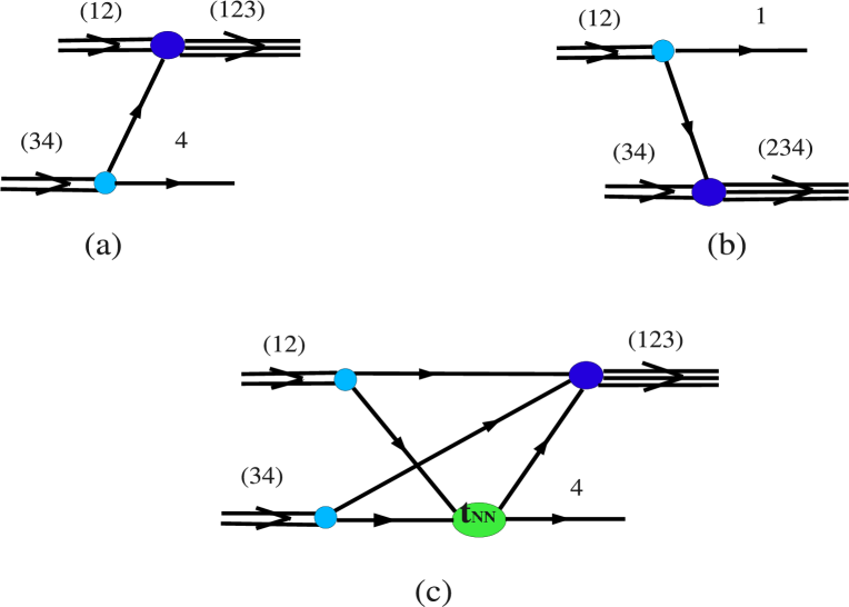
Figure 1: The diagrams taken into consideration: one-nucleon-exchange (a),(b), and single scattering (c) graphs.

2.1 One-nucleon-exchange

We start from consideration of ONE contributions. Taking the quantum numbers and momenta of all particles into account, we get the following expression for ONE terms:

$$<n{{}^{3}He}|U|dd> = \frac{1}{\sqrt{6}}<\vec{p}_{n}m_{n}\tau_{n}|<\Psi^{123}(\vec{P}_{h}M_{h}\tau_{h})|(2E_{d}-\hat{H}_{12})|\Phi^{12}(\vec{P}_{1},M_{1})>|\Phi^{34}(\vec{P}_{2},M_{2})>-$$ (21)

$$<\vec{p}_{n}m_{n}\tau_{n}|<\Psi^{234}(\vec{P}_{h}M_{h}\tau_{h})|(2E_{d}-\hat{H}_{34})|\Phi^{12}(\vec{P}_{1},M_{1})>|\Phi^{34}(\vec{P}_{2},M_{2})>.$$

Here we introduce notation $\Psi^{ijk}(\vec{P}_{h},M_{h},\tau_{h})$ for the ${}^{3}He$ wave function, where ${}^{3}He$ is formed by $i,j,k$ nucleons and has momentum $\vec{P}_{h}$, spin projection $M_{h}$ and isospin projection $\tau_{h}$. Note in case $\tau=-1/2$ we deal with the reaction of $dd\to tp$. The $\Phi^{ij}(\vec{P},M)$ denotes the wave function of the deuteron with momentum $\vec{P}$ and spin projection $M$.

Inserting the unit operator into Eq.(21):

$$1=\int d\vec{p}_{1}d\vec{p}_{2}d\vec{p}_{3}|\vec{p}_{1}m_{1}\tau_{1},\vec{p}_{2}m_{2}\tau_{2},\vec{p}_{3}m_{3}\tau_{3}><\vec{p}_{1}m_{1}\tau_{1},\vec{p}_{2}m_{2}\tau_{2},\vec{p}_{3}m_{3}\tau_{3}|~{},$$ (22)

for ONE contribution we get

$$<n{{}^{3}He}|U|dd> = \frac{1}{\sqrt{6}}\int d\vec{p}_{1}d\vec{p}_{2}d\vec{p}_{3}$$

$$(E_{d}-E_{n}-E_{3})<\Psi^{123}(\vec{P}_{h}M_{h}\tau_{h})|\vec{p}_{1}m_{1}\tau_{1};\vec{p}_{2}m_{2}\tau_{2};\vec{p}_{3}m_{3}\tau_{3}>$$

$$<\vec{p}_{1}m_{1}\tau_{1};\vec{p}_{2}m_{2}\tau_{2}|\Phi^{12}(\vec{P}_{d},M_{1})><\vec{p}_{3}m_{3}\tau_{3};\vec{p}_{n}m_{n}\tau_{n}|\Phi^{34}(-\vec{P}_{d},M_{2})>-$$

$$- \frac{1}{\sqrt{6}}\int d\vec{p}_{2}d\vec{p}_{3}d\vec{p}_{4}$$

$$(E_{d}-E_{n}-E_{2})<\Psi^{234}(\vec{P}_{h}M_{h}\tau_{h})|\vec{p}_{2}m_{2}\tau_{2};\vec{p}_{3}m_{3}\tau_{3};\vec{p}_{4}m_{4}\tau_{4}>$$

$$<\vec{p}_{n}m_{n}\tau_{n};\vec{p}_{2}m_{2}\tau_{2}|\Phi^{12}(\vec{P}_{d},M_{1})><\vec{p}_{3}m_{3}\tau_{3};\vec{p}_{4}m_{4}\tau_{4}|\Phi^{34}(-\vec{P}_{d},M_{2})>~{}.$$

Table 1: Quantum numbers of the partial waves included into the definition of the three-body wave function. $T,S,{\cal L},J$ refer to the isospin, spin, orbital momentum and total angular momentum of the NN-subsystem. $l$ is the relative orbital momentum of the spectator and $K$ is the channel spin [20].

$\nu$	Label	Subsystem	${\cal L}$	S	$J^{\pi}$	$T$	K	l
1	${}^{1}s_{0}S$	${}^{1}s_{0}$	0	0	$0^{+}$	1	1/2	0
2	${}^{3}s_{1}S$	${}^{3}s_{1}$	0	1	$1^{+}$	0	1/2	0
3	${}^{3}s_{1}D$	${}^{3}s_{1}$	0	1	$1^{+}$	0	3/2	2
4	${}^{3}d_{1}S$	${}^{3}d_{1}$	2	1	$1^{+}$	0	1/2	0
5	${}^{3}d_{1}D$	${}^{3}d_{1}$	2	1	$1^{+}$	0	3/2	2

Henceforth, we imply summations over all dummy discrete indices.

In our calculation we use the parameterized wave function of a three-nucleon system offered in ref.[20]. This wave function was derived by fitting the full Faddeev wave function obtained with the CD Bonn [21] and Paris [22] NN-potentials. The wave function is fully antisymmetrized and defined in terms of the nucleon pair and spectator momenta. If we choose particles (12) as a pair and particle 3 as a spectator, the three-nucleon wave function is presented in the following form:

$$<\vec{p}_{0}\vec{q}\nu|\Psi> = <\vec{p}_{0}\vec{q}\nu|\psi[(12)3]>+<\vec{p}_{0}\vec{q}\nu|\vec{p}_{23}\vec{q}_{1}\nu_{23}><\vec{p}_{23}\vec{q}_{1}\nu_{23}|\psi[(23)1]>+$$

$$+ <\vec{p}_{0}\vec{q}\nu|\vec{p}_{31}\vec{q}_{2}\nu_{31}><\vec{p}_{31}\vec{q}_{2}\nu_{31}|\psi[(31)2]>.$$

Here the following notations have been introduced for pair relative momentum $\vec{p}_{0}$ and spectator momentum $\vec{q}$

$$\vec{p}_{0} = \frac{\vec{p}_{1}-\vec{p}_{2}}{2},~{}~{}~{}~{}~{}\vec{q}=\vec{p}_{3}-\frac{\vec{P}}{3},~{}~{}~{}~{}\vec{P}=\vec{p}_{1}+\vec{p}_{2}+\vec{p}_{3}=\vec{P}_{h}$$

$$\vec{p}_{23} = \frac{\vec{p}_{2}-\vec{p}_{3}}{2},~{}~{}~{}~{}~{}\vec{q}_{1}=\vec{p}_{1}-\frac{\vec{P}}{3}$$ (25)

$$\vec{p}_{31} = \frac{\vec{p}_{3}-\vec{p}_{1}}{2},~{}~{}~{}~{}~{}\vec{q}_{2}=\vec{p}_{2}-\frac{\vec{P}}{3}~{}.$$

The radial part of the three-nucleon wave function (2.1) is presented as a sum of the two terms each of them has a separable form:

$$<p_{0}q\nu|\Psi>=v^{\nu}_{1}(p_{0})w^{\nu}_{1}(q)+v^{\nu}_{2}(p_{0})w^{\nu}_{2}(q),$$ (26)

where $v^{\nu}_{\lambda}(p_{0})$, $w^{\nu}_{\lambda}$ are defined as:

$$v^{\nu}_{\lambda}(p_{0})=\sum_{n=1}^{5}\frac{a^{\nu}_{n,\lambda}}{p_{0}^{2}+(m^{\nu}_{n,\lambda})^{2}}~{},~{}~{}~{}~{}~{}w^{\nu}_{\lambda}(q)=\sum_{n=1}^{5}\frac{b^{\nu}_{n,\lambda}}{q^{2}+(M^{\nu}_{n,\lambda})^{2}}~{},~{}~{}~{}~{}~{}~{}~{}~{}~{}\lambda=1,2~{}.$$ (27)

Index $\nu$ denotes number of one of the three-nucleon channels (Table 1). The five channels are included into the definition of the wave function: ${{}^{1}s}_{0}S,{{}^{3}s}_{1}S,{{}^{3}}s_{1}D,{{}^{3}d}_{1}S,{{}^{3}d}_{1}D$. Parameters $a^{\nu}_{n,\lambda},b^{\nu}_{n,\lambda},m^{\nu}_{n,\lambda}$ and $M^{\nu}_{n,\lambda}$ can be found in [20].

The wave function of the deuteron, which contains $(ij)$ nucleons, is denoted in Eq.(21) as $\Phi(\vec{P}_{d},M_{d})$. Here $\vec{P}_{d}$ and $M_{d}$ are momentum and spin projection of the deuteron, respectively. In the rest frame the non-relativistic wave function of the deuteron depends only on one variable $\vec{p}_{0}$ which is the relative momentum of the proton- neutron pair:

$$<\vec{P}_{d}/2+\vec{p}_{0},m_{p};\vec{P}_{d}/2-\vec{p}_{0}m_{n}|\Phi(\vec{P}_{d}M_{d})>=$$ (28)

$$\sum_{L=0,2}u_{L}(p_{0})<\frac{1}{2}m_{p}\frac{1}{2}m_{n}|1M_{s}><LM_{L}1M_{s}|1M_{d}>Y_{L}^{M_{L}}(\hat{p}_{0})~{},$$

where $u_{0}(p_{0})$ and $u_{2}(p_{0})$ describe $S$ and $D$ components of the deuteron wave function [21], [23], $\hat{p}_{0}$ is the unit vector in $\vec{p}_{0}$ direction, and $m_{p},~{}m_{n}$ are the proton and neutron spin projections, respectively.

Using transformations of vectors $\vec{p}_{1},~{}\vec{p}_{2},~{}\vec{p}_{3}$ to Jacobi variables (2.1) and taking into account momentum conservations in the deuterons and helium vertices, we get the following expression for the first term in Eq.(21):

$${\cal J}^{ONE}_{dir} = <\frac{1}{2}M_{h}\frac{1}{2}m_{n}|T^{ONE}_{dir}|1M_{1}1M_{2}>=$$

$$\frac{(-1)^{1/2-\tau_{h}}}{\sqrt{2}}{\cal K}\int d\hat{p}_{0}dp_{0}p_{0}^{2}\psi^{\nu}(p_{0},q){Y_{l}^{\mu}}^{*}(\hat{q}){Y_{\cal L}^{\cal M}}^{*}(\hat{p}_{0})<{\cal LM}1M_{S}|JM_{J}>$$

$$<JM_{J}\frac{1}{2}m_{3}|KM_{K}><l\mu KM_{K}|\frac{1}{2}M_{h}><\frac{1}{2}m_{3}\frac{1}{2}m_{n}|1M^{\prime}_{S}><LM_{L}1M_{S}|1M_{1}>$$

$$<L^{\prime}M^{\prime}_{L}1M^{\prime}_{S}|1M_{2}>u_{L}(p_{0})Y_{L}^{M_{L}}(\hat{p}_{0})u_{L^{\prime}}(|\vec{P}_{h}-\vec{P}_{d}/2|)Y_{L^{\prime}}^{M_{L}^{\prime}}(\widehat{\vec{P}_{h}-\vec{P}_{d}/2})$$

with kinematical factor ${\cal K}$ defined as

$${\cal K}=E_{d}-E_{n}-\sqrt{m_{N}+(\vec{P}_{h}-\vec{P}_{d})^{2}}.$$ (30)

Definitions Eq.(2.1) and (28) have been also used to obtain this equation. Superscribe index $\nu$ of the helium wave function marks one of the five channels considered in [20] and defined by quantum numbers of the nucleon pair $({\cal L},J)$, the relative orbital momentum of the spectator $l$ and the channel spin $K$ [24] (Table 1). We also preserve here the dependence on isotopic number $\tau_{h}$ that allows us to consider both $dd\to{{}^{3}He}n$ and $dd\to tp$ reactions. As it follows from Eq.(2.1), spectator momentum $\vec{q}$ is defined only by helium and deuteron momenta, $\vec{q}=\frac{2}{3}\vec{P}_{h}-\vec{P}_{d}$. Since only two spherical functions in Eq.(2.1) are dependent of integration angles, we can simply integrate this expression over the angular dependence of $\vec{p}_{0}$:

$${\cal J}^{ONE}_{dir}=\frac{(-1)^{1/2-\tau_{h}}}{\sqrt{2}}{\cal K}\int dp_{0}p_{0}^{2}\psi^{\nu}(p_{0},q)u_{L}(p_{0})u_{L^{\prime}}(|\vec{P}_{h}-\vec{P}_{d}/2|)<1M_{1}\frac{1}{2}m_{3}|KM_{K}>$$ (31)

$$<l\mu KM_{K}|\frac{1}{2}M_{h}><L^{\prime}M^{\prime}_{L}1M^{\prime}_{S}|1M_{2}><\frac{1}{2}m_{3}\frac{1}{2}m_{n}|1M^{\prime}_{S}>Y_{L^{\prime}}^{M^{\prime}_{L}}(\widehat{\vec{P}_{h}-\vec{P}_{d}/2}){Y_{l}^{\mu}}^{*}(\hat{q})~{}.$$

After substitution of the partial wave decomposition of the helium wave function [20], we get the final expression for the direct term of the ONE-contribution:

$${\cal J}^{ONE}_{dir}=\frac{(-1)^{1/2-\tau_{h}}}{\sqrt{2}}{\cal K}\int dp_{0}p_{0}^{2}\{\frac{u_{0}(|\vec{P}_{h}-\vec{P}_{d}/2|)}{\sqrt{4\pi}}<\frac{1}{2}m_{3}\frac{1}{2}m_{n}|1M_{2}>+$$ (32)

$$u_{2}(|\vec{P}_{h}-\vec{P}_{d}/2|)Y_{2}^{M^{\prime}_{L}}(\widehat{\vec{P}_{h}-\vec{P}_{d}/2})<2M^{\prime}_{L}1M^{\prime}_{S}|1M_{2}><\frac{1}{2}m_{3}\frac{1}{2}m_{n}|1M^{\prime}_{S}>\}$$

$$\{\frac{1}{\sqrt{4\pi}}[u_{0}(p_{0})\psi_{2}(p_{0},q)+u_{2}(p_{0})\psi_{4}(p_{0},q)]<1M_{1}\frac{1}{2}m_{3}|\frac{1}{2}M_{h}>+$$

$$[u_{0}(p_{0})\psi_{3}(p_{0},q)+u_{2}(p_{0})\psi_{5}(p_{0},q)]Y_{2}^{\mu~{}*}(\hat{q})<1M_{1}\frac{1}{2}m_{3}|\frac{3}{2}M_{K}><2\mu\frac{3}{2}M_{K}|\frac{1}{2}M_{h}>\}~{}.$$

This expression contains only four components of the helium wave function, since channel $\nu=1$ corresponds to the isotriplet state of the pair which is forbidden for the ONE-mechanism.

In order to get the exchange term of the ONE-amplitude ${\cal J}^{ONE}_{exch}$, it is necessary to replace $\vec{P}_{d}\to-\vec{P}_{d}$ and $M_{1}\longleftrightarrow M_{2}$ in the previous expression.

2.2 Single scattering

The single-scattering term in Eq.(18) can be rewritten in a more evident form:

$${\cal J}^{SS} = \int d\vec{p}_{1}d\vec{p}_{2}d\vec{p}_{3}d\vec{p}_{4}d\vec{p}_{1}^{\prime}<\Psi^{123}(\vec{P}_{h}M_{h}\tau_{h})|\vec{p}_{1}^{\prime}m_{1}^{\prime}\tau_{1}^{\prime};\vec{p}_{2}m_{2}\tau_{2};\vec{p}_{3}m_{3}\tau_{3}>$$

$$<\vec{p}_{1}^{\prime}m_{1}^{\prime}\tau_{1}^{\prime};\vec{p}_{n}m_{n}\tau_{n}|T(2E_{d}-E_{2}-E_{3})|\vec{p}_{1}m_{1}\tau_{1};\vec{p}_{4}m_{4}\tau_{4}>$$

$$<\vec{p}_{1}m_{1}\tau_{1};\vec{p}_{2}m_{2}\tau_{2}|\Phi^{12}(\vec{P}_{d},M_{1})><\vec{p}_{3}m_{3}\tau_{3};\vec{p}_{4}m_{4}\tau_{4}|\Phi^{34}(-\vec{P}_{d},M_{2})>.$$

We have here five integration vectors but three of them can be removed due to the momentum conservation. We introduce vectors $\vec{k}_{0}$ and $\vec{k}_{0}^{\prime}$ which correspond to the neutron-proton relative momenta in the deuterons:

$$\vec{k}_{0}=\frac{1}{2}(\vec{p}_{1}-\vec{p}_{2}),~{}~{}~{}~{}\vec{k}_{0}^{\prime}=\frac{1}{2}(\vec{p}_{3}-\vec{p}_{4}).$$ (34)

As it is mentioned above, we have used the three-nucleon wave function in a separable form which depends on two variables: $\vec{p}_{0}$, a relative momentum of a pair, and spectator momentum $\vec{q}$. In our calculations it is convenient to choose the nucleon pair (23) as a cluster and nucleon 1 as a spectator. It is possible since our wave function is symmetrized:$\Psi^{123}=\Psi^{231}$. Then the arguments of the helium wave function are expressed via momenta $\vec{k}_{0}$ and $\vec{k}_{0}^{\prime}$:

$$\vec{p}_{0}=\frac{1}{2}(\vec{P}_{d}-\vec{k}_{0}-\vec{k}_{0}^{\prime})~{}~{}~{}~{}\vec{q}=\frac{2}{3}\vec{P}_{h}+\vec{k}_{0}-\vec{k}_{0}^{\prime}.$$ (35)

Using the definitions of ${}^{3}He$ and deuteron wave functions, Eqs.(2.1 ),(28), we can write the following expression for the SS-term:

$${\cal J}^{SS}=<\frac{1}{2}M_{h}\frac{1}{2}m_{n}|T^{SS}|1M_{1}1M_{2}>=$$

$$\frac{(-1)^{1-\tau_{1}-\tau_{3}}}{2}\int d\vec{k}_{0}d\vec{k}_{0}^{\prime}\psi^{\nu}(p_{0},q)Y_{l}^{\mu}(\hat{q})^{*}Y_{\cal L}^{\cal M_{L}}(\hat{p}_{0})^{*}<l\mu KM_{K}|\frac{1}{2}M_{h}>$$

$$<{\cal LM_{L}}SM_{S}|JM_{J}><JM_{J}\frac{1}{2}m_{1}^{\prime}|KM_{K}><\frac{1}{2}m_{2}\frac{1}{2}m_{3}|SM_{S}>$$

$$<TM_{T}\frac{1}{2}\tau_{1}^{\prime}|\frac{1}{2}\tau_{h}><\frac{1}{2}-\tau_{1}\frac{1}{2}\tau_{3}|TM_{T}><\frac{1}{2}\tau_{1}^{\prime}\frac{1}{2}-\tau_{h}|T^{\prime}M^{\prime}_{T}><\frac{1}{2}\tau_{1}\frac{1}{2}-\tau_{3}|T^{\prime}M^{\prime}_{T}>$$

$$<\vec{P}_{h}+\vec{k}_{0}-\vec{k}_{0}^{\prime},m_{1}^{\prime};-\vec{P}_{h},m_{n}|T(2E_{d}-E_{2}-E_{3})|\vec{P}_{d}/2+\vec{k}_{0},m_{1};-\vec{P}_{d}/2-\vec{k}_{0}^{\prime},m_{4}>$$

$$<\frac{1}{2}m_{1}\frac{1}{2}m_{2}|1{\cal M}><LM_{L}1{\cal M}|1M_{1}>u_{L}(k_{0})Y_{L}^{M_{L}}(\hat{k}_{0})$$ (36)

$$<\frac{1}{2}m_{3}\frac{1}{2}m_{4}|1{\cal M}^{\prime}><L^{\prime}M_{L}^{\prime}1{\cal M}^{\prime}|1M_{2}>u_{L^{\prime}}(k_{0}^{\prime})Y_{L^{\prime}}^{M_{L}^{\prime}}(\hat{k}_{0}^{\prime})~{}.$$

The nucleon-nucleon scattering is described by the T-matrix element. We use the parameterization of this matrix offered by Love and Franey [25]. This is the on-shell NN T-matrix defined in the center-of-mass:

$$<\mbox{\boldmath$\kappa$}^{*\prime}\mu_{1}^{\prime}\mu_{2}^{\prime}|t_{c.m.}|\mbox{\boldmath$\kappa$}^{*}\mu_{1}\mu_{2}>=<\mbox{\boldmath$\kappa$}^{*\prime}\mu_{1}^{\prime}\mu_{2}^{\prime}|A+B(\mbox{\boldmath$\sigma_{1}$}\hat{N}^{*})(\mbox{\boldmath$\sigma_{2}$}\hat{N}^{*})+$$ (37)

$$C(\mbox{\boldmath$\sigma_{1}$}+\mbox{\boldmath$\sigma_{2}$})\cdot\hat{N}^{*}+D(\mbox{\boldmath$\sigma_{1}$}\hat{q}^{*})(\mbox{\boldmath$\sigma_{2}$}\hat{q}^{*})+F(\mbox{\boldmath$\sigma_{1}$}\hat{Q}^{*})(\mbox{\boldmath$\sigma_{2}$}\hat{Q}^{*})|\mbox{\boldmath$\kappa$}^{*}\mu_{1}\mu_{2}>.$$

The orthonormal basis $\{\hat{q}^{*},\hat{Q}^{*},\hat{N}^{*}\}$ is a combination of the nucleon relative momenta in the initial $\kappa$^∗ and final $\kappa$^′∗ states:

$$\hat{q}^{*}=\frac{\mbox{\boldmath$\kappa$}^{*}-\mbox{\boldmath$\kappa$}^{*\prime}}{|\mbox{\boldmath$\kappa$}^{*}-\mbox{\boldmath$\kappa$}^{*\prime}|},~{}~{}\hat{Q}^{*}=\frac{\mbox{\boldmath$\kappa$}^{*}+\mbox{\boldmath$\kappa$}^{*\prime}}{|\mbox{\boldmath$\kappa$}^{*}+\mbox{\boldmath$\kappa$}^{*\prime}|},~{}~{}\hat{N}^{*}=\frac{\mbox{\boldmath$\kappa$}^{*}\times\mbox{\boldmath$\kappa$}^{*\prime}}{|\mbox{\boldmath$\kappa$}^{*}\times\mbox{\boldmath$\kappa$}^{*\prime}|}.$$ (38)

The amplitudes $A,B,C,D,F$ are the functions of the center-of-mass energy and scattering angle. The radial parts of these amplitudes are taken as a sum of Yukawa terms. A new fit of the model parameters [26] was done in accordance with the phase-shift-analysis data SP07 [27].

Since the matrix elements are expressed via the effective $NN$-interaction operators sandwiched between the initial and final plane-wave states, this construction can be extended to the off-shell case allowing the initial and final states to get the current values of $\kappa$ and $\kappa^{\prime}$. Obviously, this extrapolation does not change the general spin structure.

In order to relate c.m.s. and the frame of our calculations, first of all, we apply Lorentz transformations to kinematical variables. Let us consider momenta and energies of the colliding nucleons:

$$\vec{p}_{1} = \mbox{\boldmath$\kappa$}^{*}+\vec{u}\left(\frac{(\vec{u}\mbox{\boldmath$\kappa$}^{*})}{\gamma+1}+E^{*}\right),~{}~{}~{}~{}~{}E_{1}=\gamma E^{*}+(\vec{u}\mbox{\boldmath$\kappa$}^{*})$$ (39)

$$\vec{p}_{4} = -\mbox{\boldmath$\kappa$}^{*}+\vec{u}(\frac{-(\vec{u}\mbox{\boldmath$\kappa$}^{*})}{\gamma+1}+E^{*}),~{}~{}~{}E_{4}=\gamma E^{*}-(\vec{u}\mbox{\boldmath$\kappa$}^{*}),$$

where $E^{*}$ is the energy of one of the nucleons in c.m.s. By $u=(\gamma,\vec{u})$ we denote the 4-velocity of the reference frame relatively c.m.s:

$$\vec{u}=\frac{\vec{p}_{1}+\vec{p}_{4}}{\sqrt{s}},~{}~{}\gamma=\frac{E_{1}+E_{4}}{\sqrt{s}}.$$ (40)

Mandelstam variable $s$ is defined as usual:

$$\sqrt{s}=2E^{*}=\sqrt{(E_{1}+E_{4})^{2}-(\vec{k}_{0}-\vec{k}_{0}^{\prime})^{2}}$$ (41)

Then two-nucleon state in the reference frame can be related with that in the c.m.s. due to rotations in the spin space of these nucleons:

$$|\vec{p}_{1}m_{1}>|\vec{p}_{4}m_{4}>={\cal N}|\mbox{\boldmath$\kappa$}^{*}m_{1}^{\prime}>|-\mbox{\boldmath$\kappa$}^{*}m_{4}^{\prime}>D_{m_{1}^{\prime}m_{1}}(\vec{u},\vec{p}_{1})D_{m_{4}^{\prime}m_{4}}(\vec{u},\vec{p}_{4}),$$ (42)

where the Wigner rotation operator is

$$D(\vec{u},\vec{p})=exp\{-i\vec{\sigma}\vec{\omega}\}=cos\frac{\omega}{2}\left(1-i\frac{\sigma[\vec{u}\times\vec{p}]}{(1+\gamma)m+E+\sqrt{s}}\right).$$ (43)

The rotation is performed around the axis $[\vec{u}\times\vec{p}]$ on the angle $\omega$ determined by

$$tg\frac{\omega}{2}=\frac{|\vec{u}\times\vec{p}|}{(1+\gamma)m+E+\sqrt{s}}$$ (44)

After transformations (39) the two-nucleon relative momentum in c.m.s. $\mbox{\boldmath$\kappa$}^{*}$ is written as follows:

$$\mbox{\boldmath$\kappa$}^{*}=\frac{\vec{P}_{d}}{2}+\frac{\vec{k}_{0}(E_{4}+\sqrt{s})+\vec{k}_{0}^{\prime}(E_{1}+\sqrt{s}/2)}{E_{1}+E_{4}+\sqrt{s}}~{}.$$ (45)

Likewise we can obtain an expression for the relative momentum of the scattered nucleon pair:

$$\mbox{\boldmath$\kappa$}^{*\prime}=\vec{P}_{h}+\frac{(\vec{k}_{0}-\vec{k}_{0}^{\prime})(E_{n}+\sqrt{s^{\prime}}/2)}{E_{1}^{\prime}+E_{n}+\sqrt{s^{\prime}}}~{}.$$ (46)

Here we use the following definitions:

$$E_{1}=\sqrt{m^{2}+(\vec{k}_{0}+\vec{P}_{d}/2)^{2}},~{}~{}~{}~{}~{}~{}~{}E_{4}=\sqrt{m^{2}+(\vec{k}_{0}^{\prime}+\vec{P}_{d}/2)^{2}},$$ (47)

$$E_{1}^{\prime}=\sqrt{m^{2}+(\vec{P}_{h}^{2}+\vec{k}_{0}-\vec{k}_{0}^{\prime})^{2}},~{}~{}~{}~{}\sqrt{s^{\prime}}=2E^{\prime*}=\sqrt{(E_{1}^{\prime}+E_{n})^{2}-(\vec{k}_{0}-\vec{k}_{0}^{\prime})^{2}}$$

It is also necessary to take into account normalization factor ${\cal N}$ and a kinematical coefficient due to the transformation of the off-energy-shell $T$-matrix [28]. The expressions for these factors were given in detail in ref.[29].

It should be noted, that the current parameterization describes the NN-interaction in the wide energy range between 50 MeV and 1100 MeV [26]. However, at low energies ($<100$ MeV) the quality of the parameterization can not be assessed due to the lack of the experimental data. Therefore, we do not consider the single scattering contribution into $dd\to{{}^{3}}Hen$ reaction amplitude at the deuteron energy below 200 MeV, where the Faddeev calculation technique is more preferable.

Figure 2: The differential cross section at the deuteron momentum of 1.109 GeV/c as a function of t. The data are taken from [9].

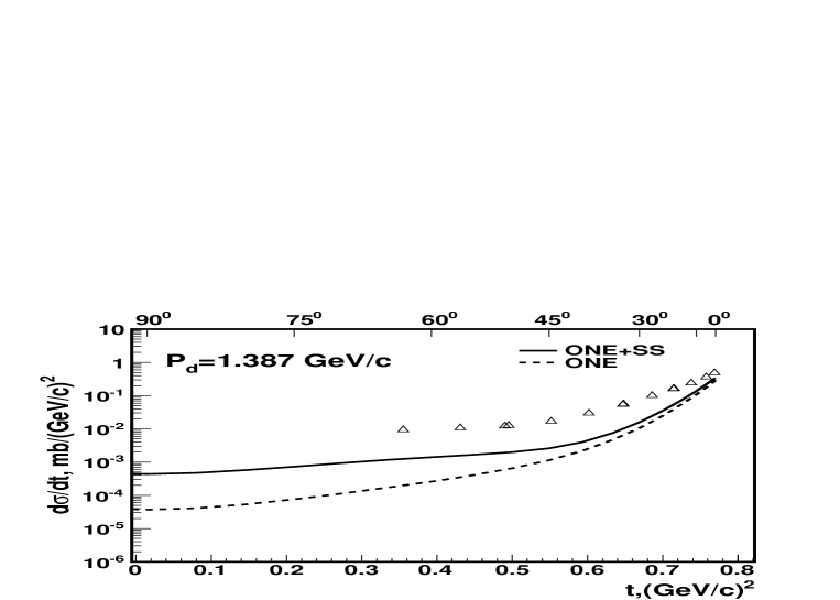
Figure 3: The differential cross section at the deuteron momentum of 1.387 GeV/c as a function of t. The data are taken from [9].

3 Results and discussions

The formalism presented above was applied to describe the experimental data obtained for $dd\to{{}^{3}Hen}$ and $dd\to tp$ reactions at the deuteron kinetic energies of a few hundred MeV. The calculations have been performed with CD-Bonn deuteron and helium wave functions. The differential cross section can be written as a function of Mandelstam variables $s$ and $t=(P_{d}-P_{He})^{2}$:

$$\frac{d\sigma}{dt}=\frac{4\pi}{9s}\frac{s^{2}-(M^{2}_{He}-m^{2})^{2}}{s-4M_{d}^{2}}|{\cal J}(s,t)|^{2}~{}.$$ (48)

We consider three energies, 300 MeV, 457 MeV and 520 MeV, which correspond to the laboratory momenta $P_{lab}=1.109,~{}1.387$, and $1.493$ GeV/c, respectively. In this energy range the presented formalism is more successful. Moreover, we have a set of the experimental data on the differential cross sections in a wide angular range obtained at these energies in Saclay [9].

In Figs.2-4 the results of the calculations of the differential cross sections are presented in comparison with the data. In order to demonstrate the contribution of the single scattering term, we have considered two cases. One of them corresponds to the calculations including only ONE terms. The results of these calculations are given with the dashed curves. The other case corresponds to the calculations taking into account both ONE and single scattering contributions. These results are presented with the solid curves.

As expected, the contribution of the rescattering term is not large at small scattering angles ($t\sim 0.7-0.8(GeV/c)^{2}$). It is in agreement with the results obtained in ref.[8]. However, the difference between these two curves increases with the angle and reaches the maximal value at $90^{0}$. Taking the single scattering diagram into consideration significantly improves the agreement between the experimental data and theoretical predictions. We have a good description of the data for $P_{lab}=1.109~{}GeV/c$ (Fig.2). Nevertheless, the underestimation of the differential cross sections is observed at the deuteron energies above 300 MeV (Figs.3,4). Perhaps, this discrepancy can be reduced, if the $\Delta$-excitation in the intermediate state is taken into account. This possibility is discussed in ref.[9], where the $\Delta$-isobar is taken into consideration in the simplest phenomenological model.

The formalism presented here gives us an opportunity to calculate not only the differential cross sections but also polarization observables. In this paper we have considered the energy dependence of tensor analyzing power $T_{20}$ at the scattering angle equal to zero (Fig.4). The experimental data were obtained at RIKEN [7]. As it is mentioned above, the contribution of the single scattering term is not large at small angles. Nevertheless, one can observe some improvement of the agreement between the data and theory predictions. Unfortunately, we do not have enough experimental data to confirm this tendency.

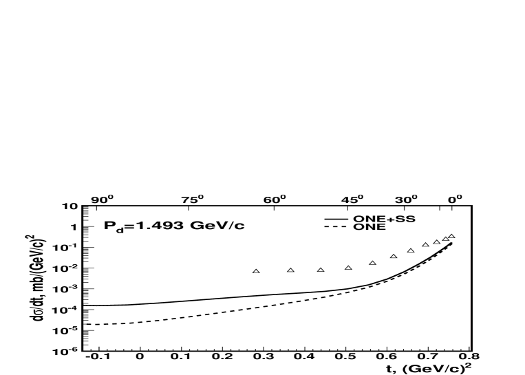
Figure 4: The differential cross section at the deuteron momentum of 1.493 GeV/c as a function of t. The data are taken from [9].

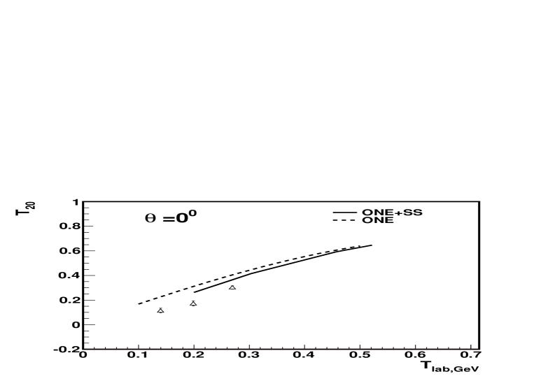
Figure 5: The energy dependence of tensor analyzing power $T_{20}$ at the zero scattering angle. The data are taken from [7]

4 Conclusions.

The model to describe the $dd\to{{}^{3}He}~{}n(tp)$ reaction at the energies of a few hundred MeV has been presented in this paper. We start from the AGS-equations for N-body system. Iterating these equations over the NN $t$-matrix we obtain the expression for the reaction amplitude. In the presented calculations only two lowest terms of this expansion are included into this consideration. Here we do not solve any equations to define wave functions of the bounded states or to find the nucleon-nucleon $t$-matrix. Instead of that the parameterized wave functions for the deuteron and helium are used. These parameterizations take the spin structure of these nuclei into account. In order to describe interactions of the nucleons in the intermediate state, the parameterized $NN$ $t$-matrix is applied that allows us to avoid the problem of convergence which appears at the partial wave decomposition at these energies.

The presented model has been applied to describe differential cross sections at deuteron energies of 300 MeV, 493 MeV, and 520 MeV. A reasonable agreement between the data and theoretical results has been obtained for the energy equal to 300 MeV. It is shown that the contribution of the single scattering term is small at the forward scattering angles while inclusion of the rescattering diagram significantly improves the description of the experimental data at the scattering angles larger than $30^{0}$. The energy dependence of the $T_{20}$ has been also obtained at the energy range between 200 MeV and 520 MeV at the zero scattering angle. Some improvement of the data description has been received when the single scattering term is taken into account. All these results allow us to regard this approach as the next step in addition to the one-nucleon-exchange mechanism to solve the four-nucleon problem.

Acknowledgements The author is grateful to Dr. V.P. Ladygin for fruitful discussions. This work has been supported by the Russian Foundation for Basic Research under grant $N^{\underline{0}}$ 10-02-00087a.

References

• [1] M.B.Epstein (1985) et al.,Phys.Rev.C 32, 967
• [2] E.J.Brash et al. (1993),Phys.Rev.C 47, 2064
• [3] P.Kitching et al. (1972), Phys.Rev.C 6, 769
• [4] A.Rahav et al. (1992),Phys.Rev.C 46, 1167
• [5] M.A. Miller et al. (1995),Phys.Rev.Lett. 74, 502
• [6] Y.Shimizu et al. (2007), Phys.Rev.C 76, 044003
• [7] V.P.Β Ladygin et al. (2004), Phys. Lett. B598 47; Phys.Atom.Nucl.69 (2006) 1271.
• [8] M.Β Janek et al. (2007), Eur.Phys.J.Β A 33 39.
• [9] G.Bizard et al. (1980),Phys.Rev.C 22, 1632
• [10] V.P.Ladygin, N.B.Ladygina (2002), Phys.Atom.Nucl. 65, 1609
• [11] V.P.Ladygin, N.B.Ladygina (1996), Phys.Atom.Nucl. 59, 789
• [12] H.M.Hofman, G.M.Hale (2008), Phys.Rev.C 77, 044002
• [13] A.Deltuva, A.C.Fonseca (2007),Phys.Rev.C 76,021001(R)
• [14] A.Deltuva, A.C.Fonseca (2010),Phys.Rev.C 81,054002
• [15] P.Grassberger, W.Sandhas (1967), Nucl.Phys.B2, 181
• [16] E.O.Alt, P.Grassberger, W.Sandhas (1970), Phys.Rev.C 1, 85
• [17] S.A.Sofianos, H.Fiedeldey, W.Sandhas (1970), Phys.Rev.C 32, 400, and refs. therein
• [18] A.M.MicherdziΕ„ska et al. (2007), Phys. Rev. C 75, 054001
• [19] M.Goldberger, K.Watson (1964) Collision Theory. Wiley, New York
• [20] V.Baru et al. (2003),Eur.Phys.J.A16, 437
• [21] R.Machleidt (2001), Phys. Rev.C 63, 024001
• [22] M. Lacombe et al. (1980), Phys.Rev.C21, 861
• [23] M. Lacombe et al. (1981), Phys.Lett.B101, 139
• [24] W.Scadow et al.(2000), Few-Body Syst. 28, 241
• [25] W.G.Love, M.A.Franey (1981), Phys. Rev.C 24, 1073
• [26] N.B.Ladygina (2008), e-preprint nucl-th/0805.3021
• [27] http://gwdac.phys.gwu.edu
• [28] H.Garcilazo (1976), Phys. Rev. C16, 1996
• [29] N.B.Ladygina, A.V.Shebeko (2003), Few-Body Syst. 33, 49